1
Introduction to Space-Time Codes
Sumeet Sandhu
Intel Corporation, M/S RNB 6-49
2200 Mission College Blvd
Santa Clara, CA 95052, USA
Rohit Nabar
ETF E119
Sternwartstrasse 7
Zurich CH8092, Switzerland
Dhananjay Gore
8465 Regents Road
Apt 436, Regents Court
San Diego, CA 92122
Arogyaswami Paulraj
Smart Antennas Research Group
Packard 272, Stanford University
Stanford, CA 94305, USA

2
I. INTRODUCTION
Optimal design and successful deployment of high-performance wireless networks present
a number of technical challenges. These include regulatory limits on usable radio frequency
spectrum and a complex time-varying propagation environment affected by fading and multi-
path. In order to meet the growing demand for higher data rates at better quality of service
(QoS) with fewer dropped connections, boldly innovative techniques that improve both spectral
efficiency and link reliability are called for. Use of multiple antennas at the receiver and trans-
mitter in a wireless network is a rapidly emerging technology that promises higher data rates at
longer ranges without consuming extra bandwidth or transmit power. This technology, popularly
known as smart antenna technology, offers a variety of leverages which if exploited correctly
can enable multiplicative gains in network performance.
Smart antenna technology provides a wide variety of options, ranging from single-input,
multiple-output (SIMO) architectures that collect more energy to improve the signal to noise
ratio (SNR) at the receiver, to multiple-input, multiple-output (MIMO) architectures that open
up multiple data pipes over a link. The number of inputs and outputs here refers to the number
of antennas used at the transmitter and receiver, respectively. Figure 1 shows a typical MIMO
system with���
transmit antennas and���
receive antennas. The space-time (S-T) modem at
the transmitter (Tx) encodes and modulates the information bits to be conveyed to the receiver
and maps the signals to be transmitted across space (���
transmit antennas) and time. The S-T
modem at the receiver (Rx) processes the signals received on each of the���
receive anten-
nas according to the transmitter’s signaling strategy and demodulates and decodes the received
signal.
Different smart antenna architectures provide different benefits which can be broadly classi-
fied as array gain, diversity gain, multiplexing gain and interference reduction. The signaling
strategy at the transmitter and the corresponding processing at the receiver are designed based on
link requirements (data rate, range, reliability etc.). For example, in order to increase the point-
to-point spectral efficiency (in bits/sec/Hz) between a transmitter and receiver, multiplexing gain
is required which is provided by the MIMO architecture. The signaling strategy also depends
on the availability of channel information at the transmitter. For example, MIMO does not re-
quire channel knowledge at the transmitter, although it enjoys improved performance if channel

3
information is available. On the other hand, spatial division multiple access (SDMA) does re-
quire channel information at the transmitter which is used to increase the network throughput at
the media access (MAC) layer. The advantage of point-to-multipoint SDMA over point-to-point
MIMO is that SDMA deploys multiple antennas only at the cellular base station or wireless local
area network (LAN) access point, thus reducing cost of the cellphone or network interface card
(NIC).
The basic smart antenna architectures are summarized in Table 1 along with different al-
gorithms that can be implemented on each architecture. Each combination of algorithm and
architecture provides a key differentiating advantage and the corresponding improvement in net-
work performance. The baseline architecture used for comparison is single-input, single-output
Metric Max range and reliability Max data rate/user Max network throughput
Gain over SISO Array gain / diversity gain Multiplexing gain Interference reduction
SIMO (� � ��� )
Rx diversity X
CCI nulling X
MISO ( ���� �
)
Tx diversity X
Beamforming X
SDMA (� �
users) X
MIMO (� � � � � )
Tx/Rx diversity X
CCI nulling X
SDMA (� �
users) X
SM (� �
streams) X
TABLE I
KEY BENEFITS (X) OF DIFFERENT SMART ANTENNA ARCHITECTURES
(SISO), i.e.����� � ��� � , where
� �is the number of transmit antennas and
���is the number
of receive antennas. The newly introduced acronyms in Table 1 are as follows : transmitter (Tx),

4
receiver (Rx), multiple-input single-output (MISO), cochannel interference (CCI), and spatial
multiplexing (SM). Note that Table 1 assumes that in order to maintain low cost analog compo-
nents, the maximum constellation size per transmit antenna cannot be increased when multiple
antennas are added. It also assumes that����� � interferers are jointly nulled for CCI reduc-
tion,� �
users are simultaneously served by SDMA, and���
data streams are transmitted over
an� � � � � MIMO link. Finally, the benefits listed are direct gains achievable with the smart
antenna techniques listed in the leftmost column. Depending on the channel conditions and
adaptation algorithms implemented at the medium access control (MAC) and physical (PHY)
layers, these direct benefits may trigger indirect cumulative gains such as improved network
throughput.
Note that while array gain, diversity gain and interference reduction are all provided by sim-
ple SIMO and MISO systems, multiplexing gain which is required to increase point-to-point
throughput is only provided by MIMO systems. In fact SIMO architectures can increase the
network throughput only if the base station uses SDMA technology. In the next few sections we
will explore the subtleties of smart antenna gains in greater depth. Starting with a simple signal
model, the basic smart antenna benefits namely array gain, diversity gain, multiplexing gain and
interference reduction will then be discussed in greater detail.
II. MULTIPLE ANTENNA CHANNEL MODEL
Consider a MIMO system with���
transmit antennas and���
receive antennas as shown in
Figure 2. For simplicity we consider only flat fading; i.e., the fading is not frequency selective.
When a continuous wave (CW) probing signal, � , is launched from the� ���
transmit antenna,
each of the���
receive antennas sees a complex-weighted version of the transmitted signal. We
denote the signal received at the ����
receive antenna by �� � , where ��� is the channel response
between the� ���
transmit antenna and the ����
receive antenna. The vector � �� ����������������������1 is the signature induced by the
� ���transmit antenna across the receive antenna array. It is�
The superscript � stands for matrix transpose.

5
convenient to denote the MIMO channel ( � ) in matrix notation as shown below.
� �
����������
� � � ����� � � ��� �� � ����� �� � �...
.... . .
...
������ ����� � ����� ����� � �
� ���������
(1)
The channel matrix � defines the input-output relation of the MIMO system and is also known
as the channel transfer function. If a signal vector � � � � � � ������ ��� � � is launched from the
transmit antenna array ( �� is launched from the� ���
transmit antenna) then the signal received at
the receive antenna array, � � � � � ������� ��� ��� can be written as
� ������� (2)
where � is the��� � � noise vector consisting of independent complex-gaussian distributed
elements with zero mean and variance � �� (white noise). Note that the above channel matrix can
be interpreted as a snapshot of the wireless channel at a particular frequency and at a specific
instant of time. When there is rich multipath with a large delay spread, � varies as a function
of frequency. Likewise, when the scatterers are mobile and there is a large doppler spread, �varies as a function of time. With sufficient antenna separation at the transmit and receive arrays,
the elements of the channel matrix � can be assumed to be independent, zero-mean, complex-
gaussian random variables (Rayleigh fading) with unit variance in sufficiently rich multipath.
This model is popularly referred to as the i.i.d Gaussian MIMO channel. In general if antennas
are separated by more than half the carrier wavelength ( � � ) [1], the channel fades can be modeled
as independent Gaussian random variables.
This point-to-point model can be extended to multiple users by indexing � as ��� where ���is the
� � � � � channel from the � ��� user to the receiver, as shown below
� � � ��������������� � ���
� �� ��� (3)
where �!� is the� � � � signal transmitted from the � ��� user. This system model can be easily
generalized to unequal numbers of transmit antennas at different users. In this chapter we will
focus on the single user case.

6
III. BENEFITS OF SMART ANTENNA TECHNOLOGY
Equipped with the mathematical system description via (2) and (3), we will now describe
different smart antenna gains in detail.
A. Array gain
Consider a SIMO system with one transmit antenna and two receive antennas as shown in
Figure 3. The two receive antennas see different versions, � and � � , of the same transmitted
signal, � . The signals � and � � have different amplitudes and phases as determined by the
propagation conditions. If the channel is known to the receiver, appropriate signal processing
techniques can be applied to combine the signals �� and � � coherently so that the resultant power
of the signal at the receiver is enhanced, leading to an improvement in signal quality. More
specifically, the SNR at the output is equal to the sum of the SNR on the individual links. This
result can be extended to systems with one transmit antenna and more than two receive antennas
as follows 2 � � �� ��� � �
� � � (4)
where the optimal��� � � linear receive filter is
�� �
, and the maximum SNR is propor-
tional to the channel norm � � � � ��� ����� � � � � , where � � � � is the Frobenius norm 3. The
average increase in receive signal power at the receiver = � � � � � is defined as array gain and is
proportional to the number of receive antennas.
Array gain can also be exploited in systems with multiple antennas at the transmitter by using
beamforming. Extracting the maximum possible array gain in such systems requires channel
knowledge at the transmitter, so that the signals may be optimally processed before transmission.
An example of transmit beamforming for ������
MISO systems is shown below
� � ��������� ��� (5)
The optimal normalized��� � � transmit filter is
�� ��� � � � . Analogous to the SIMO case, the
array gain in MISO systems with channel knowledge at the transmitter is equal to � � � � � and is
proportional to the number of transmit antennas. The array gain in MIMO systems depends on�The superscript � stands for conjugate transpose.�The Frobenius norm of a matrix � is defined to be ����� ��� � �"! #%$ & �"! # $ �

7
the number of transmit and receive antennas and is a function of the dominant singular value of
the channel.
B. Diversity gain
Signal power in a wireless channel fluctuates (or fades) with time/frequency/space. When the
signal power drops dramatically, the channel is said to be in a fade. Diversity is used in wireless
systems to combat fading. The basic principle behind diversity is to provide the receiver with
several looks at the transmitted signal over independently fading links (or diversity branches).
As the number of diversity branches increases, the probability that at any instant of time one or
more branch is not in a fade increases. Thus diversity helps stabilize a wireless link.
Diversity is available in SISO links in the form of time or frequency diversity. The use of time
or frequency diversity in SISO systems often incurs a penalty in data rate due to the utilization
of time or bandwidth to introduce redundancy. The introduction of multiple antennas at the
transmitter and/or receiver provides spatial diversity, the use of which does not incur a penalty
in data rate while providing the array gain advantage discussed earlier. In this chapter we are
concerned with this form of diversity. There are two forms of spatial diversity – receive and
transmit diversity.
Receive diversity applies to systems with multiple antennas only at the receiver (SIMO sys-
tems) [2]. Figure 3 illustrates a system with receive diversity. Signal � is transmitted from a
single antenna at the transmitter. The two receive antennas see independently faded versions, � and � � , of the transmitted signal, � . The receiver combines these signals using appropriate signal
processing techniques so that the resultant signal exhibits much reduced amplitude variability
(fading) as compared to either � or � � . The amplitude variability can be further reduced by
adding more antennas to the receiver. The diversity in a system is characterized by the number
of independently fading diversity branches, also known as the diversity order. The diversity or-
der of the system in Figure 3 is two and in general is equal to the number of receive antennas,� �
, in a SIMO system.
Transmit diversity is applicable when multiple antennas are used at the transmitter and has
become an active area for research in the past few years [3], [16], [4]. Extracting diversity
in such systems does not necessarily require channel knowledge at the transmitter. However,
suitable design of the transmitted signal is required to extract diversity. Space-time coding

8
[5], [6] is a powerful transmit diversity technique that relies on coding across space (transmit
antennas) and time to extract diversity. Figure 4 shows a generic transmit diversity scheme for a
system with two transmit antennas and one receive antenna. At the transmitter, signals � and � �are derived from the original signal to be transmitted, � , such that the signal � can be recovered
from either of the received signals �� or � � . The receiver combines the received signals in such
a manner that the resultant output exhibits reduced fading when compared to �� or � � . The
diversity order of this system is two and in general is equal to the number of transmit antennas,� �
, in a MISO system.
Utilization of diversity in MIMO systems requires a combination of receive and transmit
diversity described above. A MIMO system consists of��� � � � SISO links. If the signals
transmitted over each of these links experience independent fading, then the diversity order of
the system is given by��� � � � . Thus the diversity order in a MIMO system scales linearly with
the product of the number of receive and transmit antennas. Mathematically, diversity is defined
to be equal to the slope of the symbol error rate (SER) versus SNR graph. This will be shown in
greater detail in the following derivation.
The vector equation in (2) can be written as the following matrix equation� � ��� ��� (6)
where the channel input � is an��� ��� codeword spanning � sample times, the channel output
is the� � ��� matrix
�observed on
���receive antennas over � sample times and the receiver
noise is the� � ��� matrix � .
Consider two��� ��� codewords �� �� and ��� that are transmitted over
���transmit antennas
across � sample times. If �� �� was transmitted, the probability that ��� ��� ��� �� is detected for
a given realization of the channel � is equal to the following� � ��� � � ��� ��� � � � ���� � � �� ��� ��� � � � � ��� � � ���� � � � ��� � �� � �� � � �"!#%$ & � ('*)�+,.-/ (7)
where� � ��� �10324�5�6 7 �98;:=<*> � � � �� � is the complementary error function,
& � �@??? � � � � �� � � � � ??? ��is the pairwise Euclidean distance at the receiver and '*)�+ �BA(CDFE is the ratio of the total transmit-
ted signal power to the noise power per receive antenna.

9
This conditional pairwise error probability (PEP) is a function of the channel realization.
Since the transmitter does not know the channel, the best it can do is optimize a criterion that
takes channel statistics into account. One popular criterion is the average PEP, i.e. the average
of the conditional PEP over channel statistics. It is difficult to compute the expectation of the
expression in (7). A simpler alternative is to compute the average of a tight upper bound, in
particular the Chernoff upper bound� � ��� � � �"!# $ & � '*)�+,.-/ ������� � #����� (8)
For the i.i.d. Gaussian channel, the average Chernoff bound simplifies to the following as derived
in [4], [5]� � � � �� :�� ��� ��� �������� � � � �� � � � � � � � �� � � � � � ��� ��� � ����� � � � � ������ � �� ��� ��� (9)
where� :�� is the determinant of a square matrix, � � �! �� � are the nonzero singular values of the
difference matrix " � � ��� �� � ��� and # is its rank. Taking the limit at high SNR,
� � � � $ '*)�+%'& � ��� � � �(� � � �� � �) �� ��� �
(10)
and taking the logarithm of both sides, we have* �,+ � � � � � � � # * �,+ $ '*)�+%'& � * �,+ � �(� � � �� � �) �-� (11)
Consider the logarithm of the PEP in (11). The right hand side is clearly linear in the logarithms
of SNR and the product of squared singular values of the difference matrix. In addition, the
slope of the r.h.s. is a product of the number of receive antennas and the rank of the difference
matrix. The diversity gain of the space-time codebook is defined to be the minimum value of# over all pairs of codewords. For a given diversity gain, the coding gain is defined to be the
minimum of the product� � �� � � �� � �) over all pairs of codewords.
Performance of space-time codes is usually illustrated by plotting the SER versus SNR on a
logarithmic scale. Since the PEP is closely related to SER, (11) is a good approximation to SER
especially at high SNRs. Figure 5 illustrates the effect of each code metric on the SER curve.
Diversity gain affects the asymptotic slope of the SER versus SNR graph - greater the diversity,
the faster the SER drops with SNR. Coding gain affects the horizontal shift of the graph - greater
the coding gain, the greater the shift to the left.
10
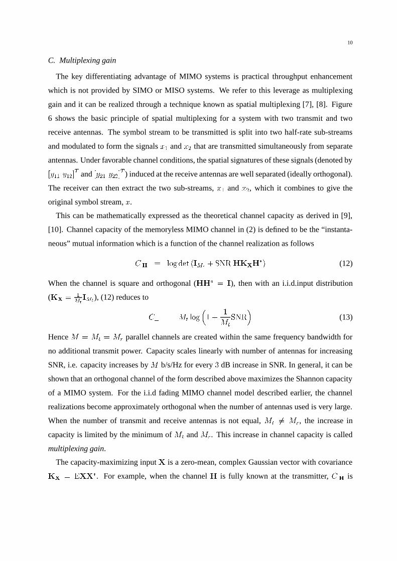
C. Multiplexing gain
The key differentiating advantage of MIMO systems is practical throughput enhancement
which is not provided by SIMO or MISO systems. We refer to this leverage as multiplexing
gain and it can be realized through a technique known as spatial multiplexing [7], [8]. Figure
6 shows the basic principle of spatial multiplexing for a system with two transmit and two
receive antennas. The symbol stream to be transmitted is split into two half-rate sub-streams
and modulated to form the signals � and � � that are transmitted simultaneously from separate
antennas. Under favorable channel conditions, the spatial signatures of these signals (denoted by
� � � � ��� and � � � � � � ��� ) induced at the receive antennas are well separated (ideally orthogonal).
The receiver can then extract the two sub-streams, � and � � , which it combines to give the
original symbol stream, � .
This can be mathematically expressed as the theoretical channel capacity as derived in [9],
[10]. Channel capacity of the memoryless MIMO channel in (2) is defined to be the “instanta-
neous” mutual information which is a function of the channel realization as follows
� � � � * �,+ � :�� ��� ��� � '*)�+ ����� � � � (12)
When the channel is square and orthogonal ( � � � � �), then with an i.i.d.input distribution
( ��� � ��� � ��� ), (12) reduces to
��� � � � * �,+ $ � � �� � '*)�+ & (13)
Hence� � � � � � �
parallel channels are created within the same frequency bandwidth for
no additional transmit power. Capacity scales linearly with number of antennas for increasing
SNR, i.e. capacity increases by�
b/s/Hz for every � dB increase in SNR. In general, it can be
shown that an orthogonal channel of the form described above maximizes the Shannon capacity
of a MIMO system. For the i.i.d fading MIMO channel model described earlier, the channel
realizations become approximately orthogonal when the number of antennas used is very large.
When the number of transmit and receive antennas is not equal,��� �� � � , the increase in
capacity is limited by the minimum of���
and� �
. This increase in channel capacity is called
multiplexing gain.
The capacity-maximizing input � is a zero-mean, complex Gaussian vector with covariance
��� � ��� � � . For example, when the channel � is fully known at the transmitter,� � �
is

11
maximized by ��� that waterpours power over the dominant singular values of � [9]. The
conditional capacity can be achieved by coding over longer and longer block lengths, assuming
that the channel is time-invariant. In practice the fading channel does vary with time, and a
commonly used measure of rate in this case is the average channel capacity. Average capacity
of the memoryless MIMO channel is defined to be the average mutual information described as
follows
� � � � � � � � � � * �,+ � :�� ��� ��� � '*)�+ ����� � � � (14)
where the average is computed over the channel distribution function. It has been shown in
[9] that the iid input distribution is optimal for the iid Gaussian channel. Figure 7 shows the
average capacity as a function of the SNR for the i.i.d fading channel model for different MIMO
configurations. It is clear that the average capacity increases with the number of antennas in the
system. At very low SNR, the MIMO multiplexing gain is low, but it increases with increasing
SNR becoming asymptotically constant.
D. Interference reduction
In contrast to copper or optical fiber, the wireless medium is an unguided communication link
as a result of which co-channel interference is a frequent problem due to the reuse of frequency
spectrum in wireless networks. CCI adds to the overall noise in the system and deteriorates per-
formance. Figure 8 illustrates the general principle of interference reduction for a receiver with
two antennas. Typically, the desired signal ( � ) and the interference ( � ) arrive at the receiver with
well separated spatial signatures - � � � � ��� and � � � � ��� respectively. The receiver can exploit the
difference in spatial signatures to reduce the interference, thereby enhancing the signal to in-
terference ratio (SIR). Interference reduction usually requires knowledge of the desired signal’s
spatial channel and benefits from knowledge of the interferers’ spatial channels. Interference
reduction can also be implemented at the transmitter via SDMA, where the goal is to enhance
the signal power at the intended receiver and minimize the interference energy sent towards the
co-channel users. Interference reduction allows the use of aggressive reuse factors and improves
network capacity.
Having discussed the key advantages of smart antenna technology we note that it may not be
possible to exploit all the leverages simultaneously in a smart antenna system. This is because

12
the spatial degrees of freedom are limited and engineering tradeoffs must be made between
each of the desired benefits. The optimal spatio-temporal signaling strategy is a function of the
wireless channel properties and network requirements.
IV. BACKGROUND ON SPACE-TIME CODES
As described in the previous section, MIMO systems promise much higher spectral efficiency
than SISO systems. MIMO systems can also be leveraged to improve the quality of transmission
(reduce error rate). This section will focus on MIMO signaling schemes that assume perfect
channel knowledge at the receiver and no channel knowledge at the transmitter.
A. Space-time trellis codes
For a given number of transmit antennas, the code design objective from (11) is to construct
the largest possible codebook with full diversity gain ( # � ��� ) and the maximum possible coding
gain. A number of hand-crafted STTCs (space-time trellis codes) with full diversity gain were
first provided in [5]. Full diversity codes with greater coding gain were then reported in [13],
where codes were found through exhaustive computer searches over a feedforward convolutional
coding (FFC) generator. New codes were then presented in [15] by searching for the codes with
the best distance spectrum properties. The distance spectrum of a codebook counts how many
pairs of codewords are located at a given product distance (defined as� � �� � � �� � �) for the � �
codeword pair in (11)).
To provide some insight into all these codes, Figures 9 and 10 show the frame error rate for
two transmit antennas over an iid Gaussian channel. As a reference, a linear space-time block
code (STBC) from [12] is also shown, with and without a concatenated AWGN trellis code
(STBC + TCM). The STBC does not provide coding gain but does provide full diversity, which
is of order, � �
for both the STBC and the STTCs considered here.
In Figure 9 (a) note that STBC by itself performs slightly better than all the STTCs, even
though it provides no coding gain. This is explained by the multidimensional structure of STBC,
i.e., each input symbol is spread over two time samples which improves performance against
AWGN. With one receive antenna, concatenated STBC performs significantly better than all the
4-state STTCs. The performance gap reduces with increasing receive antennas in Figure 10.
With three receive antennas and 8 trellis states, in fact, STTC-Yan outperforms STBC-TCM.

13
This performance loss is explained by the well-known capacity loss incurred by STBC [18], and
will be addressed in greater detail in the next section.
The performance gap between STBC-TCM and STTC is also less noticeable with 8-state
codes for all receive antennas. We conjecture that the distance spectrum of the concatenated
scheme degrades in comparison to the distance spectrum of STTC with increasing number of
TCM states. While we will not directly address the distance spectra of space-time codes here,
we will introduce a tighter error criterion than the worst-case PEP which reflects the effects of
the distance spectrum on error probability.
Let us summarize the three main observations made so far. Space-time block codes which are
linear in the input information symbols are simple to encode and decode. Since STBCs outper-
form STTCs for small number of antennas, they are of great interest in such MIMO architectures.
In general, the distance spectrum of the codebook is a better measure of error performance than
the maximum pairwise error probability, and should be incorporated into code design metrics.
Finally, linear block codes with the best error performance do not always demonstrate the best
capacity performance.
B. Linear space-time block codes
Since linear codes are easier to encode and decode, we will focus on the design of linear
codes here. A linear code is defined as a set of codewords that are linear in the scalar input
symbols. Complex valued��� � � modulation matrices ����� ��� � are used to spread the input
information symbols over��� � spatio-temporal dimensions. The real and imaginary part of each
input symbol � � is modulated separately with the matrices ��� and � ���� � . Define �� ��� � � and
� ���� � �� � � where ���� ���
. The modulated matrices are summed to obtain the��� ���
codeword � as follows
� ���� ��� � � ��� � � ��������� ��� � � � � �
��� � ��� �� (15)
The number of modulation matrices�
is usually upper bounded by the total number of spatio-
temporal degrees of freedom, ��� � . When
��� , � � � , the modulation matrices can be de-
signed to be orthogonal (as defined in (20), (21)) in order to optimize error performance as
shown in the next section. For optimal capacity performance, however, in general� � , � � �
and the modulation matrices are not orthogonal.

14
In order to normalize transmit power, the modulation matrices are scaled as follows
���� � ��������� ' � � ��� � �� ��� � , �� ����� * * ����� � ����� � ��� � �� ��� � ��� ����� * * � (16)
for different input constellations such as quadrature amplitude modulation (QAM), phase shift
keying (PSK) and pulse amplitude modulation (PAM). Most of the current spatial modulation
techniques can be interpreted as linear codes, the key exceptions being space-time trellis codes.
Example 1—Spatial multiplexing: Spatial multiplexing [7], also called BLAST [10], is the
simplest example of linear codes. Each incoming symbol is transmitted only once on one an-
tenna and at one symbol time. The modulation matrices are Kronecker delta matrices, i.e., each� � ��� matrix is equal to 1 in the �
���row and the
� ���column and zero elsewhere. For example,
for the case��� � , � � � � , the modulation matrices are as follows
� ���� � � �
� �� �
��� ��� �� � � �
��� � �� �� � � � �
��� � �� �� � �
��� ��� �� � �
Example 2—Orthogonal space-time block codes: Orthogonal space-time block codes are a
special example of linear codes, where the codeword � is designed to be a unitary matrix. Such
modulation matrices exist for limited values of�
,���
and � [6]. For example, the orthogonal
block code for��� � ,
, � � , is the Alamouti code [12] consisting of four matrices shown below
� ���� � � � ��� � � �
� �� �
��� � �� �
� �� � � �
��� � �� � �
� �� �
���� � � �� �
� �� � � � �
��� � ����
� �� � � (17)
Example 3—Delay diversity: Delay diversity [3], [16] is really a trellis code that can also be
classified as a linear code. The��� ��� modulation matrices are proportional to � ��� ��� � � , where
the order� �
identity matrix is shifted right by� � � columns in the
� ���modulation matrix.
For any ��� � � , the total number of complex symbols thus encoded is��� � � � � . The case
� � � , � � � , is shown below
� ���� � � ���� � �
� �� �
��� ���� �
� �� � � �
��� � �� �
� �� � � � �
��� � �
���� �� � ���

15
���� ���� �
� �� � �
��� � �� �
� �� � � �
��� � ���
� �� ���
This framework can be extended to non-linear codes by modulating the modulation matrices
with nonlinear functions of the input symbols. For example, for� � � , the following vector of
input symbols leads to a nonlinear space-time code������� � �� �
� ����� �
������� � � � � �
� �����
This is similar to the analytic representation of TCM [17], except that the coefficients of the
analytic expansion are now modulation matrices instead of scalars.
V. NEW DESIGN CRITERIA
In this section we will first discuss design criteria for optimizing error performance and ca-
pacity performance separately. Then we will bring the two together to design capacity-efficient
codes that also provide good error performance.
A. Error performance
Evaluating the distance spectrum of space-time codes is difficult. Optimizing their distance
spectrum is even harder, and possibly not very insightful. We propose a simple new criterion
that efficiently incorporates the effects of the distance spectrum, i.e., the union bound on error
probability. The union bound is an upper bound on average error probability, where the average
is taken over the entire matrix constellation. Moreover, the union bound is a tighter upper bound
than the worst case PEP. This follows because the union bound is an average whereas the worst
case PEP is the maximum, and can be seen from the following inequalities
��� � � � � ��� � � � ��
��� � � � � � � �� � � �� � <� � � � � (18)
for a constellation consisting of�
equally likely codewords, where � � is the probability that the
����
codeword was transmitted. Therefore it is advisable to minimize the scaled union bound, i.e.

16
� � � � , rather than the maximum PEP, i.e. � < � � � � . To provide a contrast we illustrate the
two bounds in Figure 11 for the Alamouti code and spatial multiplexing.
The union bound on error probability for linear codes can be averaged over the iid Gaussian
channel and written as follows [19]
��� � ��� � � � ��
��� � � :�� � ��� � ��� �% ��
� � �� � � ��� � ���� � � � � � � � � � � ��� (19)
where�
is the size of the codebook (� � � � � for an input M-QAM constellation), and
� � � � �
� � ��� � � � � is the difference of the input sequences � � �� and � � at the� ���
location. See [19] for a
detailed proof.
Let the modulation matrices be unitary 4, i.e. ��� � �� � � ��� for� � � � and � �� ��� � �
� for� � � � . Then we have the following necessary and sufficient condition for code design.
Theorem 1: A linear code consisting of wide unitary modulation matrices minimizes���
iff it
satisfies (20)
��� � �� ��� � � �� � � ��� � � � �� � � (20)
A linear code consisting of tall unitary modulation matrices minimizes���
iff it satisfies (21)
� �� � � ��� �� ��� � � ��� � � � �� � � (21)
See [19] for a detailed proof. This gives us the conditions required for optimal error perfor-
mance. Note that these conditions precisely describe orthogonal space-time block codes [6].
B. Capacity performance
We can rewrite the complex channel in (6) as the following real channel
� � � � � � (22)
where (, � � � � � ) is the channel output vector,
�(, ��� � � , � � � ) is the block diagonal
channel,�
(, ��� � � , � ) is the linear code matrix to be designed, � (
, � � � ) is a block of
uncoded input symbols with each entry of power ��� � , , and � (, � � � � � ) is the noise vector�
Unitary modulation matrices achieve the matched filter bound, i.e. they minimize error probability when � ��� .

17
with each entry of power��� � ,
. These quantities are defined as follows 5
� � : � ���� � � �
� �� �
� � ��� � ����� : � : � �
��� � � � � � � �
� ��
� ���� � : � !#
��� � � �
� �� -�/ � � � � : � !#
��� � � � � � � �
� �� -�/
� ��
� � � � � � � � � ��� � � � � � � � � � � � � �� � � : � �
��� � � �
� �� � (23)
and are all real. This reformulation cleanly separates the channel from the linear code, thereby
enabling us to analytically maximize channel capacity.
Average capacity of this input-output equation can be written as
� � � � �, � * �,+ � :�� ��� � ��� � � '*)�+ � � � � � � � (24)
Theorem 2: In order to maximize the average channel capacity over all normalized linear
codes�
for any number of receive antennas, it is sufficient that the optimal linear code�
satisfy the following factorization
� � ������� � � (25)
where�
is a (, � � ��� ) factor of the input covariance ��� � � � � � ��� � , and � is any
( � � � , � ) unitary matrix such that ��� � � �(where � � � , � ). See [19] for a detailed proof.
If the channel is i.i.d.Gaussian, then average capacity is maximized by choosing � � ��� � � ��� �[9]. In this case,
�is a unitary matrix and the optimal linear code is unitary. A code that
maximize average channel capacity is called capacity-efficient. For the i.i.d.Gaussian channel,
any code that satisfies� � � � � � � � � is capacity-efficient. Note that Theorem 2 is a sufficient
condition to design capacity-efficient codes for any number of receive antennas. This condition
is not necessary for limited cases, e.g. the Alamouti code does not satisfy Theorem 2 but is��������� ��� is the column-by-column vectorization of matrix � , is the matrix kronecker product, and ! is the entrywise
complex conjugate of ! .

18
capacity-efficient for one receive antenna (it is not capacity-efficient for two or more receive
antennas).
C. Unified design
In this section we will put together the criteria derived in the previous two sections to design
new linear space-time block codes. First, define the following metrics for code design :
� Deviation from unitarity is defined as follows
5 � ����� � � � ����� � � (26)
where � is the condition number with respect to the spectral norm. When each of the
modulation matrices is unitary, 5 � � .� Deviation from pairwise skew-Hermitianity is defined as follows
5 � � �� ���� � � ��� � �� ��� � � �� � �� (27)
where � � � �� is the squared Frobenius norm. When all the modulation matrices are pairwise
skew-Hermitian, 5 � � � , and when they also satisfy 5 � � , the code is error-optimal.
� Deviation from capacity-efficiency is defined as follows
5 � � � � � � � �� �
� � �� (28)
When 5 � � � , the code is capacity-efficient for any number of receive antennas. For codes
that are capacity-efficient for limited values of���
, such as the Alamouti code with one
receive antenna, it is possible that 5 ��� � .Using these metrics, we will design capacity-efficient codes that also perform well with respect
to error probability. Our method of code generation is via random search, which is explained in
detail in the following.
We will focus on the case of two transmit antennas and block length of two. The minimum
number of modulation matrices required for capacity-efficient codes is� � , ��� � ��� . A large
number of real,� � � random matrices with zero-mean, unit-variance Gaussian entries were
generated, their singular value decompositions were computed, and their left singular matrix
was extracted as a candidate for the code matrix�
. Since the left singular matrix is orthogonal

19
by definition, it is automatically capacity-efficient and 5 � � � . For each such code, its non-zero
deviations 5 and 5 � were evaluated. After evaluating all candidate codes, we chose a good code
that had the lowest values of both 5 and 5 � over the ensemble generated.
The performance of this chosen code is demonstrated over the i.i.d. Gaussian channel by
means of simulated BER in Figure 12 for two receive antennas and a data rate of 4 bits per
sample time. The new code is labeled “random CE” and is evaluated against other capacity-
efficient codes such as spatial multiplexing (“SM”) and Linear Dispersion (“LD”). For reference
we have also plotted the performance of the Alamouti code (“STBC”). With two receive antennas
and a rate of eight bits per codeword, CE outperforms both LD and SM at high SNRs. At a BER
of �� ���
, CE is at an advantage of about 5 dB. It therefore has a much higher diversity than
LD and SM, although not as much as STBC which outperforms all these codes at high enough
SNRs. In Figure 13, with three receive antennas CE outperforms STBC by about 1 dB at a BER
of �� � �
.
What this demonstrates is that all capacity-efficient codes don’t perform equally well with
respect to BER, and that the modulation matrices must also be pairwise skew-Hermitian and
unitary in order to minimize BER. Note that in general, the relative performance of these codes
is a function of SNR, number of receive antennas and data rate, and a code that is the best for a
given set of conditions may not be the best under different conditions.
For reference we have reproduced the LD code [14]
� � �, ��� � �� �
� �� � � � � �, ��� � �� �
� ��
� � � �, ��� � � �� �
� �� � � � � �, ��� � �
� � �� ��
� � � �, ��� � � �� � �
� �� � ��� � �, ��� � �
� �� ��
��� � �, ��� � � �� �
� �� � ��� � �, ��� � � �
� �� �� (29)
and our new CE code below
� ���� � � ,�� % � � � � � � � � � � � ,� � � � � � � � , � �� � , � � , � � � � � % � � � � � � � � � � � , ��� �
� ��

20
� � ���� � � � , � � % � � � � � � � � � � ,�, � � � � � � ��� , �� � � ,�� � � � � ,���� � � � � � � � � � � % � � � �
� ��
� � ���� � � � , � , � � � � � � � � � � , � � � � � � � � % , �� � ,�, � % � � � � � � � � � � � % % � � � � , % ,�� �
� ��
� � ���� � � � , % � � � � � % � � � � � � � , � � � � , ��� � �� � � � % � � � � � � � � , � � � � ,�� % � � � � ,� % � �
� ��
� � ���� � � ��� ��� � � � ��� % � � � � � , � � � � � � � � � �� � � %,% � , � � � � � � � � � � � % � � � � ,�� � � �
� ��
��� ���� � � � � � � � � � � % � � � � � � � � � � � � � � � � �� � � � � � � � � � , � � � � � � � � � � � � � � , � � � �
� ��
��� ���� � � , � , � � � � ����� � � � % � � � � � � � ,�,� �� � � � � � , � � � % ,���� � � � � � � % � � � � � ��� �
� ��
��� ���� � � � ,�� � � � � � , � � � � � � � � ��� % � � � � � � �� � � , � � � � � � � % � % � � � � � , � � � � � � � � � �
� �� (30)
What is interesting about this code is that the singular values of all modulation matrices are
very similar and are listed in Table 6.1. This suggests that non-unitary modulation matrices may
Matrix �� ��� � � �� � ���� 0.6843 0.1784 3.84
� � 0.6847 0.1769 3.87
� � 0.6867 0.1685 4.08
� � 0.6642 0.2428 2.74
� � 0.6472 0.2846 2.27
��� 0.6691 0.2288 2.93
��� 0.6754 0.2094 3.23
��� 0.6358 0.3094 2.06
TABLE II
SINGULAR VALUES FOR “RANDOM CE”
outperform unitary modulation matrices in some cases. The relative importance of different

21
design metrics may be determined by formal minimization of the average union bound on error
probability and will not be addressed here.
VI. RECEIVER DESIGN
For a general MIMO channel, the receiver receives a superposition of the transmitted signals
and must separate the constituent signals based on channel knowledge. The method of spatial
deconvolution determines the computational complexity of the receiver. This problem is similar
in nature to the multi-user detection problem in CDMA and parallels can be drawn between the
receiver architectures in these two areas.
The signal design in this chapter assumed maximum likelihood (ML) decoding, which amounts
to exhaustive comparisons of the received signal to all possible transmitted signals. This is com-
putationally prohibitive for higher order constellations such as 64-QAM, which for example
would require� % � � % �����
complex multiplications, Euclidean distance computations and com-
parisons for two transmit antennas. While ML detection is optimal, receiver complexity grows
exponentially with the number of transmit antennas making this scheme impractical. Lower
complexity sub-optimal receivers include the zero-forcing receiver (ZF) or the minimum mean-
square error (MMSE) receiver, the design principles of which are similar to equalization prin-
ciples for SISO links with inter-symbol interference (ISI). An attractive alternative to ZF and
MMSE receivers is the vertical BLAST (V-BLAST) algorithm described in [11], which is es-
sentially a successive cancellation technique. An exciting new algorithm that yields ML-like
performance with cubic instead of exponential complexity is the sphere decoding algorithm
[20].
A. Modulation and coding for MIMO
The signal design in this chapter did not include effects of concatenated coding. MIMO
technology is compatible with a wide variety of coding and modulation schemes. In gen-
eral, the best performance in achieved by generalizing standard (scalar) modulation and coding
techniques to matrix channels. MIMO has been proposed for single-carrier (SC) modulation,
direct-sequence code division multiple access (DS-CDMA) and orthogonal frequency division
multiplexing (OFDM) modulation techniques. MIMO has also been considered in conjunction
with concatenated coding schemes. Application of turbo codes and low density parity codes to

22
MIMO has recently generated a great deal of interest, as have simpler coding and interleaving
techniques such as bit-interleaved coded modulation (BICM) along with iterative decoding. In-
clusion of concatenated codes along with soft Viterbi decoding is in fact essential for realizing
the full diversity gain of practical MIMO systems.
VII. CONCLUDING REMARKS
Smart antenna wireless communication systems provide significant gains in terms of spectral
efficiency and link reliability. These benefits translate to wireless networks in the form of im-
proved coverage and capacity. MIMO communication theory is an emerging area and full of
challenging problems. Some promising research areas in the field of MIMO technology include
channel estimation, new coding and modulation schemes, low complexity receivers, MIMO
channel modeling and multiuser SDMA network design.
REFERENCES
[1] W. C. Y. Lee, Mobile Communications Engineering, New York: Mc-Graw Hill, 1982.[2] W. C. Jakes, Microwave Mobile Communications, New York: Wiley, 1974.[3] A. Wittneben, Base station modulation diversity for digital SIMULCAST, Proc. IEEE VTC: 505-511, May 1993.[4] J. Guey, M. Fitz, M. Bell, and W. Kuo, Signal design for transmitter diversity wireless communication systems over
Rayleigh fading channels, Proc. IEEE VTC: 136-140, 1996.[5] V. Tarokh, N. Seshadri, and A. R. Calderbank, Space-time codes for high data rate wireless communication: Performance
criterion and code construction, IEEE Trans. Inf. Theory, vol.44: 744-765, March 1998.[6] V. Tarokh, H. Jafarkhani, and A. R. Calderbank, Space-time block codes from orthogonal designs, IEEE Trans. Inf. Theory,
vol.45: 1456-1467, July 1999.[7] Increasing capacity in wireless broadcast systems using distributed transmission/directional reception, US Pat. 5,345,599,
A. J. Paulraj and T. Kailath.[8] G. J. Foschini, Layered space-time architecture for wireless communication in a fading environment when using multi-
element antennas, Bell Labs Tech. J.: 41-59, Autumn 1996.[9] I. E. Telatar, Capacity of multi-antenna gaussian channels, Tech. Rep. #BL0112170-950615-07TM, AT&T Bell Laborato-
ries, 1995.[10] G. J. Foschini and M. J. Gans, On limits of wireless communications in a fading environment when using multiple antennas,
Wireless Personal Comm., vol.6, no.3: 311-335, Netherlands: Kluwer Academic Publishers, 1998.[11] G. D. Golden, G. J. Foschini, R. A. Valenzuela, and P. W. Wolniansky, Detection algorithm and initial laboratory results
using the V-BLAST space-time communication architecture, Electronic Letters, vol. 35, no.1: 14-15, 1999.[12] S. M. Alamouti, A simple transmit diversity technique for wireless communications, IEEE J. Sel. Areas Comm., vol.16:
1451-1458, October 1998.[13] J. Grimm, Transmitter diversity code design for achieving full diversity on Rayleigh fading channels, Ph.D. Thesis, Purdue
University : 1998.[14] B. Hassibi and B. M. Hochwald, High-rate codes that are linear in space and time, Proc. 38th Annual Allerton Conference
on Communication, Control and Computing : 2000.[15] Q. Yan and R. S. Blum, Optimum space-time convolutional codes, Proc. WCNC : 2000.[16] N. Seshadri and J. H. Winters, Two signaling schemes for improving the error performance of frequency-division-duplex
(FDD) transmission systems using transmitter antenna diversity, Vehicular Technology Conference : 508-11, 1993.[17] E. Biglieri and D. Divsalar and P. J. McLane and M. K. Simon, Introduction to Trellis-Coded Modulation with Applications
: 1991.[18] S. Sandhu and A. Paulraj, Space-time block codes : a capacity perspective, IEEE Communication Letters : vol 4, 384-86,
2000.[19] S. Sandhu, Signal design for multiple-input multiple-output wireless : a unified perspective, Ph.D. Thesis, Stanford Uni-
versity : 2002.[20] E. Viterbo and J. Bouros, A universal lattice code decoder for fading channels IEEE Trans. Information Theory : vol 45,
1639-1642, 1999.

23

24
Acronym ExpansionAWGN additive white Gaussian noise
BER bit error rateBICM bit interleaved coded modulation
BLAST Bell Labs layered space-time transceiverCCI co-channel interference
CDMA code division multiple accessCE capacity efficientCW continuous waveDS direct sequence
i.i.d. independent, identically distributedLAN local area networkLD linear dispersion
MAC media access layerMIMO multiple input, multiple outputMISO multiple input, single output
ML maximum likelihoodMMSE minimum mean squared error
NIC network interface cardOFDM orthogonal frequency division multiplexingPAM pulse amplitude modulationPEP pairwise error probabilityPHY physical layerPSK phase shift keying
QAM quadrature amplitude modulationQoS quality of serviceRx receiveSC single carrier
SDMA spatial division multiple accessSER symbol error rate
SIMO single input, multiple outputSISO single input, single outputSM spatial multiplexing
SNR signal to noise ratioSTBC space time block codeSTTC space time trellis codes.v.d. singular value decompositionTCM trellis coded modulation
Tx transmitZF zero forcing
TABLE III
GLOSSARY

25
Space-Time Modem
Space-Time Modem
Transmit Antenna Array Receive Antenna Array
1
2
1
2
Tx Rx
Input Bit Stream Output Bit Stream
M T M R
Fig. 1. Schematic of a MIMO Communication System
Tx
Rx
s
SNR = SNR + SNR
1
2 out 1 2
s out
s 1
s 2
Scatterers
Fig. 2. Array Gain

26
Rx
Tx
s s 1
s 2
s out Scatterers
Fig. 3. Receive Diversity
Rx s
Tx
Scatterers
s 1
s 2
s 11
s 21
s out
Fig. 4. Transmit Diversity

27
SER (log scale)
SNR (in dB)
uncoded
diversity gain
coding gain
Fig. 5. Diversity gain and coding gain
Rx Tx s 1
s 2
Scatterers
s 1,out
s 2,out
s 11 s 21 s 1
s 2
s 22 s 12
Fig. 6. Spatial Multiplexing

28
−10 0 10 20 30 40 5010
−1
100
101
102
Average channel capacity − i.i.d. matrix fading channels
SNRS in dB
Cap
acity
in b
its /
sec
/ Hz
20x209x9 3x3 2x2 1x1
Fig. 7. Capacity
Rx
Interference (i)
Desired Signal (s)
s 1
s 1
s 2
i 1
i 1
s 2 i 2
i 2
s out
s out
i out
i out
Scatterers
Fig. 8. Interference Reduction

29
10 12 14 16 1810
−3
10−2
10−1
100
(a) 4 state codes
SNR in dB
FE
R
STBC STBC + 4−state TCMGrimm 4−state Yan 4−state
10 12 14 16 1810
−3
10−2
10−1
100
(b) 8 state codes
SNR in dB
FE
R
STBC STBC + 8−state TCMGrimm 8−state Yan 8−state
Fig. 9. One receive antenna

30
0 2 4 6 810
−3
10−2
10−1
100
(a) 4 state codes
SNR in dB
FE
R
STBC STBC + 4−state TCMGrimm 4−state Yan 4−state
0 2 4 6 810
−3
10−2
10−1
100
(b) 8 state codes
SNR in dB
FE
R
STBC STBC + 8−state TCMGrimm 8−state Yan 8−state
Fig. 10. Three receive antennas

31
0 5 10 15 20 25 30 3510
−6
10−5
10−4
10−3
10−2
10−1
100
Union bound (solid) versus maximum PEP (dotted) (1x2, 4 b/s/Hz)
SNR (dB)
Uni
on b
ound
/(R
−1)
and
max
imum
PE
P
Alamouti codeSpatial Multiplexing
Fig. 11. Union bound compared to maximum PEP

32
5 10 15 20 25 3010
−7
10−6
10−5
10−4
10−3
10−2
10−1
100
SNR in dB
BE
R
Mr = 2, M
t = 2, 8 bits/codeword
STBCSMLDrandom CE
Fig. 12. BER for 2 receive antennas

33
0 2 4 6 8 10 12 14 16 18 20 2210
−7
10−6
10−5
10−4
10−3
10−2
10−1
100
SNR in dB
BE
R
Mr = 3, M
t = 2, 8 bits/codeword
STBCα2 = 7/8α2 = 6/8α2 = 5/8α2 = 4/8LDrandom CESM
Fig. 13. BER for 3 receive antennas
Recommended