Intracellular Viral Life-cycle Induced Rich
Dynamics in Tumor Virotherapy
Jianjun Paul Tian1, Yang Kuang2, Hanchun Yang3
1Department of Mathematics
The College of William and Mary, Williamsburg, VA 231872 School of Mathematical and Statistical Sciences
Arizona State University, P.O. Box 871804 Tempe, AZ 852873 Department of Mathematics
Yunnan University, Kunming 650091, PR China
Emails: [email protected], [email protected], [email protected]
Abstract
The intracellular viral life-cycle is an important process in tumor
virotherapy. Most mathematical models for tumor virotherapy do not
incorporate the intracellular viral life-cycle. In this article, a model for
tumor virotherapy with the intracellular viral life-cycle is presented
and studied. The period of the intracellular viral life-cycle is mod-
eled as a delay parameter. The model is a nonlinear system of delay
differential equations. It displays interesting and rich dynamic behav-
iors. There exists two sets of stability switches as the period of the
intracellular viral life-cycle increases. One is around the infection free
equilibrium solution, and the other is the positive equilibrium solution.
This intracellular viral life-cycle may explain the oscillation phenom-
ena observed in many studies. An important clinic implication is that
the period of the intracellular viral life-cycle should also be modified
when a type of a virus is modified for virotherapy, so that the period of
the intracellular viral life-cycle is in a suitable range which can break
away the stability of the interior equilibrium solution.
1

1 Introduction
The old hypothesis of viruses can be used to kill tumor cells has been ex-
tensively restudied over last 20 years. Oncolytic viruses have been identified
in many experiences [3]. Viruses that can infect and replicate in cancer
cells but leave healthy cells unharmed can serve as oncolytic viruses. In
an ideal situation, when oncolytic viruses are inoculated into a cancer pa-
tient or directly injected into a tumor, they spread throughout the tumor,
and infect tumor cells. The viruses that enter into tumor cells will repli-
cate themselves. Upon a lysis of an infected tumor cell, a swarm of new
viruses burst out and infect neighboring tumor cells. It was hypothesized
that all tumor cells would be infected and the tumor would be eradicated
since the beginning of the nineteenth century [8]. However, most often the
viral infection was stopped by the host immune system and failed to im-
pact on tumor growth. The later technology of reverse genetics has brought
about new methods to generate tumor-selective viruses, and progresses in
understanding of the molecular mechanism of viral cytotoxicity of oncolytic
viruses may provide a fascinating therapeutic approach to cancer patients.
Recent experiments in animal brain tumors using genetically engineered vi-
ral strains, such as adenovirus, ONYX-15 and CV706, herpes simplex virus
1 and wild-type Newcastle disease virus show these viruses to be relatively
non-toxic and tumor specific [9]. However, the therapeutic effects of these
oncolytic viruses are not well established yet.
There are many factors that influence the efficacy of tumor virotherapy.
The major factors include the intracellular viral life-cycle and viral repli-
cation within tumor cells, viral localization or virus distribution within a
tumor, and the immune responses that viral infection induce [12]. Many
experiments with animals and phase I clinical trials have been conducted
to investigate these factors. For example, a great deal of the intracellular
viral life cycle has been found out experimentally. In [3], the intracellular
viral life cycle for adenovirus and herpes simplex virus (HSV)-1 is detailed,
“the life cycle can be divided into several stages. During the infection stage,
2

viral surface proteins, such as the adenovirus fibre or HSV glycoprotein D,
mediate attachment to cellular receptors, such as coxsackie and adenovirus
receptor (CAR) or HSV entry mediator C (HVEC), also known as nectin
1. Once inside the cell, viruses express several gene products that target
cellular proteins and modulate various cellular processes, such as preventing
apoptosis or inducing cell-cycle entry. These promote viral replication and
production of viral proteins that eventually lead to cell lysis and release of
viral progeny”. Each step is mediated by a diverse group of proteins, and
each step needs some time to complete [6, 7, 4, 13]. However, an integrated
and quantitative understanding of viral kinetics is required in order to find
predictive factors for the efficacy of virotherapy. Without such an under-
standing, much of the clinical research will continue to be based on trial
and error. In this aspect, mathematical modeling can allow us to see the
whole spectrum of possible outcomes, and provide the rationale to optimize
treatments. Several attempts have been made to understand and character-
ize viral dynamics by mathematical models [5, 14, 16, 15, 17, 18, 19, 1, 20].
These studies are largely of qualitative simulation in nature and examine
how variation in viral and host parameters influences the outcomes of treat-
ments. The outcomes of virotherapy depend in a complex way on interac-
tions between viruses and tumor cells. A clearer picture of the dynamics of
virotherapy needs to be developed.
Based on experimental results in [10] that glioma-selective HSV-1 mu-
tants (rQNestin34.5) have a high replication ability and doubles the life span
of glioma mice. The studies in [5, 14] have suggested that viral replication
ability is one of major factors for the success of virotherapy. The model
in [5] studies interactions among glioma cells, infected glioma cells, viruses,
immune cells, and also includes the immunosuppressive agent, cyclophos-
phamide. It is a nonlinear parabolic system with a free boundary as tumor
surface. The study of a space-free virotherapy model in [14] suggests that
the oscillation is an intrinsic property of virotherapy dynamics and relates to
virus replication ability. The present paper focuses on analyzing the effect of
the intracellular viral life-cycle on the dynamics of oncolysis in a relatively
3
simpler setting and will only consider tumor cells and viruses in a space-free
setting.
The rest of the article is organized as follows. In Section 2, the mathe-
matical model is introduced. In Section 3, preliminary results on the model
are presented. In Section 4, the stability of the equilibrium solutions is stud-
ied, and some numerical analysis is also presented. In Section 5, we conclude
the paper by a discussion of biological implications of our results.
2 Mathematical models
Wodarz and Komarova in [11, 18, 19] proposed the following general model
of tumor cell and infected tumor cell growth based on the mass action law,
x′ =dx
dt= xF (x, y)− βyG(x, y),
y′ =dy
dt= βyG(x, y)− ay,
(1)
where x stands for the uninfected tumor cell population and y the infected
tumor cell population. The function F describes the growth properties of the
uninfected tumor cells with F (0, 0) representing their maximum growth rate,
and the function G describes the rate at which tumor cells become infected
by the virus. These two functions may take various forms, depending on how
much detail of the biology is incorporated into the model. The coefficient
β represents the strength of infectivity of the virus via infected tumor cells.
The infected tumor cells die at a rate ay. We would like to point out that
this is a reduced basic framework to describe the dynamics of virotherapy.
Generally, infected tumor cells can not infect uninfected tumor cells directly;
only free viruses that are in extracellular matrix can infect tumor cells. For
this reason, the above model shall be understood as an approximation of
4

the following model with explicit virus dynamics
x′ =dx
dt= xF (x, y)− bvg(x, y),
y′ =dy
dt= bvg(x, y)− ay,
v′ =dy
dt= ky − dv,
(2)
where min{k, d} >> F (0, 0), and βyG(x, y) = bkd yg(x, y). Here vg(x, y)
describes the contact rate of virus with uninfected tumor cells, b is the
virus infection coefficient (rate), k stands for the virus production rate of an
infected cell and d is the death rate of virus. In other words, one may take
advantage of the fact that virus dynamics is usually much faster than that
of tumor cell by approximating v with kdy in the above model.
There are several stages in a typical viral life-cycle. The first stage is the
attachment stage. When a free virus is within a certain distance of a tumor
cell, chemical bonds form between the virus and receptor sites of the tumor
cell, and then attach to tumor cell surface. The second is the penetration
stage, where the viral DNA passes through the core and into the tumor
cell. Once the virus penetrates into the tumor cell, the biosynthesis stage
begins. Since the virus expresses several gene products that target cellular
proteins and modulate various cellular processes, the host protein synthesis
stop and the host transcription and translation are interfered. Meantime,
the virus uses host nucleotides to replicate its DNA and use host ribosomes,
enzymes and amino acids to synthesize its enzymes and proteins. During
the maturation stage, viral capsids are assembled, viral DNA are packed
into the heads and tails fibers are joined to the complexes. The last step is
the release stage. The newly-born viruses are released from the tumor cell,
and the tumor cell dies. The time period of the intracellular viral life-cycle
varies according to virus species, it changes from minutes to days. For the
details of the viral life-cycle, we refer the reader to [3, 6, 7, 4, 13] While
it may not be necessary to include all details of the viral life-cycle into a
mathematical model where we are mainly interested in tumor dynamics to
void complication, it is interesting to find out what dynamics maybe induced
5

by the intracellular viral life-cycle in a tumor virotherapy. A simple way to
study the intracellular viral life-cycle induced dynamics is to incorporate a
cycle time delay parameter in a plausible model.
Let the cycle time of the intracellular viral life-cycle be τ , defined to be
the period of time from a virus attaching to a tumor cell to new viruses
bursting out. We assume a constant death rate for infected but not yet
virus-producing tumor cells to be n. Then the probability of infected tumor
cells surviving the time period from t− τ to t is e−nτ . (More generally, the
survival probability is given by some nonincreasing function p(τ) between
0 and 1.) For simplicity, we lump the natural death of infected tumor cells
and death by bursting together. This yields
dx
dt= xF (x, y)− βyG(x, y),
dy
dt= βy(t− τ)G(x(t− τ), y(t− τ))e−nτ − ay.
In the following, we take F (x, y) = r(1 − x+yK ) and G(x, y) = x, where r is
per capital growth rate of the tumor, and K is the maximum of the tumor
cell load. Therefore, the model we will focus on is given by,
dx
dt= rx(1− x+ y
K)− βxy,
dy
dt= βx(t− τ)y(t− τ)e−nτ − ay,
x(θ) ≥ 0, y(θ) ≥ 0, are continuous on [−τ, 0),
x(0) > 0, y(0) > 0.
(3)
3 Preliminaries
For the convenience of analysis, we non-dimensionalize the system by setting
x = xK , y = y
K , and then drop the bar over the variables. We get the non-
dimensionalized system,
6

dx
dt= rx(1− x− y)− bxy,
dy
dt= bx(t− τ)y(t− τ)e−nτ − ay,
x(θ) ≥ 0, y(θ) ≥ 0, x(θ), y(θ) ∈ C[−τ, 0],
(4)
where b = βK. We remark that all parameters here are nonnegative.
As an epidemiology model at the cell population level, the basic repro-
duction number is given by
R0 =β
ae−nτ =
b
aKe−nτ .
However, we will not use this quantity as a critical value to characterize the
dynamics of the model (4), since there is the parameter τ presenting the
period of the intracellular viral life-cycle, and we are more interested in how
this parameter affects the dynamics.
We will study the feasible region and positivity of the solutions of this
system, and the existence of equilibrium solutions.
Proposition 3.1. Let 0 ≤ x(θ), y(θ) ≤ 1 for θ ∈ [−τ, 0), and x(0) > 0,
y(0) > 0. Then the solution of the system (4) x(t) > 0, y(t) > 0, and
x(t) < 1. When x(0) + y(0) < 1, we have x(t) + y(t) < 1 + bre−nτ for t ≥ 0.
Proof. When 0 ≤ t ≤ τ , we see that y′ = bx(t − τ)y(t − τ)e−nτ − ay ≥−ay, so y(t) > y(0)e−at > 0. In addition, x′ = rx(1 − x − y) − bxy, so
x(t) = x(0)e∫ t0 r(1−x(s)−y(s)−
bry(s))ds > 0. By the method of steps, x(t) > 0
and y(t) > 0 for all t > 0.
For x′ = rx(1− x− y)− bxy < rx(1− x), so, x(t) < 1.
For 0 ≤ t ≤ τ , adding the two equations of the system (4) together, we
have x′+ y′ = rx(1−x− y)− bxy+ be−nτx(t− τ)y(t− τ)− ay ≤ rx(1−x−y)− bxy+ be−nτ −ay ≤ rx(1−x−y) + be−nτ ≤ r(1 + b
re−nτ −x−y). When
x(0) + y(0) < 1, by a standard comparison argument, we have x(t) + y(t) <
1 + bre−nτ . By the method of steps, the estimate holds for t ≥ 0.
7

Therefore, We will consider our system over this region, and the global
word will refer to this region.
The system always has equilibria (0, 0) and (1, 0) for any values of pa-
rameters. The interior equilibrium solution (x∗, y∗) is given by
E∗ = (x∗(τ), y∗(τ)) = (a
benτ ,
1− ab enτ
1 + br
).
It should be noticed that the interior equilibrium is a function of the model
parameters, and we will mainly consider it as a function of delay parameter
τ .
Since the time delay parameter τ can not be negative in our case, when
b ≤ a, there are only two nonnegative equilibria, (0, 0) and (1, 0). When
b > a, there are two cases. If 0 < τ < 1n ln b
a , there are three nonnegative
equilibria. At τ = 1n ln b
a , the interior equilibrium (x∗, y∗) merges to (1, 0).
If τ > 1n ln b
a , the interior equilibrium has negative components and goes out
of the feasible region. We will not consider this case. So, when τ ≥ 1n ln b
a ,
there are only two nonnegative equilibria, (0, 0) and (1, 0).
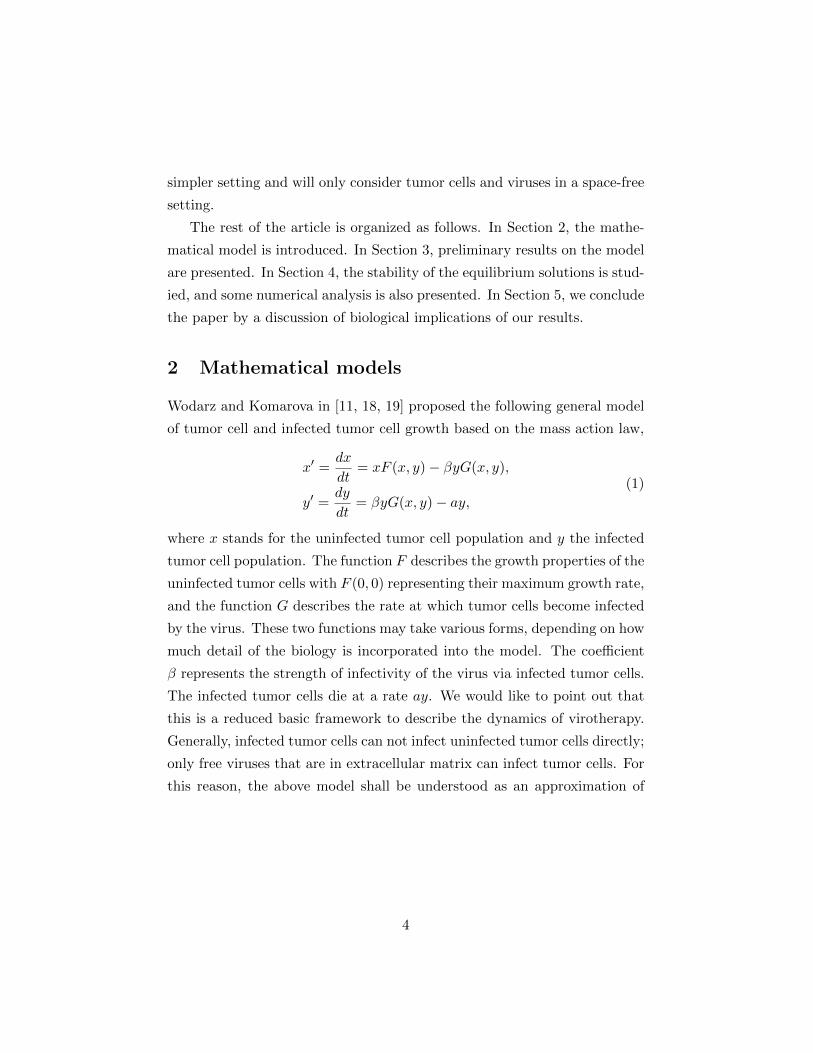
The Figure 1 shows the planar analysis of isoclines and the interior equi-
librium curve as the delay parameter τ. It also makes clear how the interior
equilibrium point (x∗(τ), y∗(τ)) depends on the delay τ and other parame-
ters. For instant, increasing τ moves the y-isoline towards right, and causes
the coincidence of (x∗(τ), y∗(τ)) with (1, 0) at a finite value of τ . For large τ
there is no positive interior equilibrium point. We will track how the interior
equilibrium depends on the parameters in all our analysis.
4 Analysis of the model
In this section, the local stability analysis of the three equilibria and some
global stability analysis will be conducted. The stability switches around
the equilibria (1, 0) and (x∗(τ), y∗(τ)) will also be studied.
8
Figure 1: For various values of the delay parameter τ , the isoclines of the
system are obtained from (4) by removing the delay parameters from the
argument. The arrows indicate the y-isoclines change as τ increases, while
the dots indicate equilibria.
4.1 Stability of the equilibrium (0, 0)
At the equilibrium point (0, 0), the linearization is
dx
dt= rx,
dy
dt= −ay.
The eigenvalues are r and −a. It is a saddle point. The stable manifold is in
y−aixs, and the unstable manifold is in x−axis. This means that the tumor
will grow when it starts with a very small size, while the tumor with only
infected cells will shrink to zero.
9
4.2 Stability of the equilibrium (1, 0)
At the equilibrium point (1, 0), we linearize the system by setting x = 1 + x
and y = y, we have
x′ = −rx− ry − rx2 − rxy − by + · · ·,
y′ = −ay + by(t− τ)e−nτ + bx(t− τ)y(t− τ)e−nτ .
The linear system then is given by(x′
y′
)=
(−r −r − b0 −a
)(x
y
)+
(0 0
0 be−nτ
)(x(t− τ)
y(t− τ)
). (5)
The characteristic equation is |λI − A − Be−λτ | = 0, where the matrices
A and B are given in (5). Or, (λ + r)(λ + a − be−nτe−λτ ) = 0. So, one
eigenvalue is −r, the other eigenvalues are given by
λ+ a− be−nτe−λτ = 0. (6)
We study the roots of the equation (6) according to the relation between
a and b. Denote the root by λ(τ) = α(τ) + iω(τ).
When b < a, λ(0) = b − a < 0. Suppose λ = iω is a root of (6), where
ω > 0. Then, substitute it into (6), we have iω+a−be−nτe−iωτ = 0. Separate
the real parts and imaginary parts. One has, ω + be−nτ sinωτ = 0 and
a− be−nτ cosωτ = 0. By sin2 ωτ + cos2 ωτ = 1, one gets b2e−2nτ = ω2 + a2.
Then, ω2 = b2e−2nτ − a2 < 0. This is impossible. Therefore, the sign of
the real part of the root λ(τ) keeps unchangeable for all τ ≥ 0. Namely,
α(τ) < 0 for any τ ≥ 0. In this case, the equilibrium point (1, 0) is locally
asymptotical stable for any (zero or positive) delay. Consequently, there is
no stability switches around the equilibrium point (1, 0) when b < a. For
the details about stability switching, we refer the paper [2] by Beretta and
Kuang.
If a = b, we claim that the real part of any root of the characteristic
equation (6) is negative. Suppose λ = u + iv, then substitute it into the
equation. Separate the real part and imaginary part, we have u + a −
10

ae−(n+u)τ cos vτ = 0 and v + ae−(n+u)τ sin vτ = 0. Square them and add
them together, we have (u + a)2 + v2 = a2e−2(n+u)τ . For any τ > 0 and
positive parameter n, if u > 0, then (u + a)2 + v2 > a2 and a2e−2(n+u)τ <
a2. This is a contradiction. If u = 0, we arrive the same contradiction.
Therefore, when a = b, the equilibrium (1, 0) is still asymptotically stable
for any positive delay τ > 0.
When b > a, λ(0) = α(0) + iω(0) = b− a > 0. Then, there is a positive
eigenvalue at τ = 0. We search for the values of the delay τ at which the sign
of the real part of λ(τ) changes, where we have stability switches. Suppose
λ = iω is a root, ω > 0. One again obtains iω + a − be−nτe−iωτ = 0.
Separate the real part and imaginary part, we have ω + be−nτ sinωτ = 0
and a− be−nτ cosωτ = 0, and ω2 = b2e−2nτ − a2. Then
ω(τ) = (b2e−2nτ − a2)12 ,
where τ < τc = 1n ln b
a . When τ > τc, there is no stability switches. As the
method in [2], we define the angle θ(τ) ∈ [0, 2π] which are the solutions of
the equations for the real part and imaginary part as follows,
sin θ(τ) = −ω(τ)
benτ , cos θ(τ) =
a
benτ .
It is easy to see that θ(τ) is in between 32π and 2π since a, b, and ω are
positive. So, θ(τ) = 2π − arcsin ω(τ)b enτ . We define
τm(τ) =θ(τ) + 2mπ
ω(τ)=
2(m+ 1)π − arcsin√b2e−2nτ−a2enτ
b√b2e−2nτ − a2
for m ∈ N0. The occurrence of stability switches may take place at the zeros
of the functions
Sm := τ − τm(τ), m ∈ N0. (7)
To determine how many zeros of the functions (7) can have, we study
the function
Zm(τ) = τ√b2e−2nτ − a2 + arcsin
enτ
b
√b2e−2nτ − a2 − 2(m+ 1)π. (8)
11
The function (8) has the same zeros as the function (7). The derivative of
the function (8) is given by
Z ′m =b2(1− nτ)e−2nτ − a2(n+ 1)√
b2e−2nτ − a2. (9)
The critical points of Zm, namely zeros of Z ′m are the same as its numerator,
b2(1−nτ)e−2nτ −a2(n+1) = 0. Then we have (2−2nτ) = 2a2(n+1)b2
e2nτ . By
simply plotting functions y = 2−x and y = Aex, it is easy to conclude that
there is only one positive critical point for Zm when a2(n+1)b2
< 1, there is
only one zero critical point when a2(n+1)b2
= 1, and there is only one negative
critical point when a2(n+1)b2
> 1. Since there is only one critical point, it easy
to check at the critical point the function Zm reaches its global maximum.
Denote the critical point by τc, we arrive the conclusion that there will be
two positive zeros for the function Sm when a2(n+1)b2
< 1 and Zm(τc) > 0 for
some m. Although there would be one positive zero for Sm when a2(n+1)b2
≥ 1
and Zm(0) > 0 for some m, we know the number of zeros of Sm only can be
an even number.
To determine the ranges of parameter values where the pair of simple
conjugate purely imaginary roots crosses the imaginary axis from left to right
or from right to left, we use the theorems 3.1 and 3.2 in [2] to determine
the sign of the derivative of the eigenvalue with respective to τ , R(τ) =
sign{dReλdτ |λ=iω(τ∗)}, and
R(τ) =sign {a2(τ)ω(τ)ω′(τ)(a(τ)b(τ) + c(τ)2τ)
+ ω2(τ)a2(τ)(a′(τ)b(τ)− a(τ)b′(τ) + c2(τ))},
where a(τ) = 1, b(τ) = a and c(τ) = −be−nτ for the characteristic equation
(6). Then we have
R(τ) = sign {ωω′(a+ b2e−2nττ) + ω2b2e−2nτ}
= sign {b2e−2nτ (−na− a2 − nb2τe−2nτ + b2e−2nτ )}
= sign {b2e−2nτ [−a(a+ n) + (1− nτ)b2e−2nτ ]}
Therefore, R(τ) = +1 if and only if (1−nτ)e−2nτ > a(a+n)b2
, and R(τ) = −1
if and only if (1− nτ)e−2nτ < a(a+n)b2
.
12
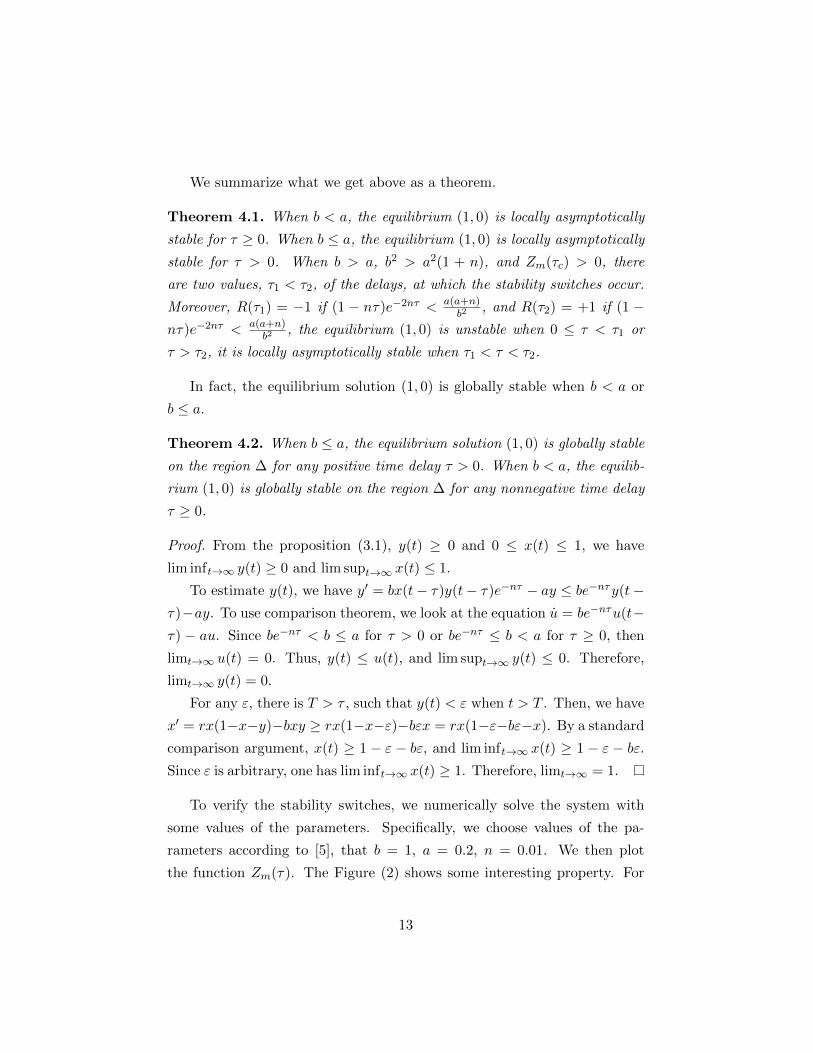
We summarize what we get above as a theorem.
Theorem 4.1. When b < a, the equilibrium (1, 0) is locally asymptotically
stable for τ ≥ 0. When b ≤ a, the equilibrium (1, 0) is locally asymptotically
stable for τ > 0. When b > a, b2 > a2(1 + n), and Zm(τc) > 0, there
are two values, τ1 < τ2, of the delays, at which the stability switches occur.
Moreover, R(τ1) = −1 if (1 − nτ)e−2nτ < a(a+n)b2
, and R(τ2) = +1 if (1 −nτ)e−2nτ < a(a+n)
b2, the equilibrium (1, 0) is unstable when 0 ≤ τ < τ1 or
τ > τ2, it is locally asymptotically stable when τ1 < τ < τ2.
In fact, the equilibrium solution (1, 0) is globally stable when b < a or
b ≤ a.
Theorem 4.2. When b ≤ a, the equilibrium solution (1, 0) is globally stable
on the region ∆ for any positive time delay τ > 0. When b < a, the equilib-
rium (1, 0) is globally stable on the region ∆ for any nonnegative time delay
τ ≥ 0.
Proof. From the proposition (3.1), y(t) ≥ 0 and 0 ≤ x(t) ≤ 1, we have
lim inft→∞ y(t) ≥ 0 and lim supt→∞ x(t) ≤ 1.
To estimate y(t), we have y′ = bx(t− τ)y(t− τ)e−nτ − ay ≤ be−nτy(t−τ)−ay. To use comparison theorem, we look at the equation u = be−nτu(t−τ) − au. Since be−nτ < b ≤ a for τ > 0 or be−nτ ≤ b < a for τ ≥ 0, then
limt→∞ u(t) = 0. Thus, y(t) ≤ u(t), and lim supt→∞ y(t) ≤ 0. Therefore,
limt→∞ y(t) = 0.
For any ε, there is T > τ , such that y(t) < ε when t > T . Then, we have
x′ = rx(1−x−y)−bxy ≥ rx(1−x−ε)−bεx = rx(1−ε−bε−x). By a standard
comparison argument, x(t) ≥ 1 − ε − bε, and lim inft→∞ x(t) ≥ 1 − ε − bε.Since ε is arbitrary, one has lim inft→∞ x(t) ≥ 1. Therefore, limt→∞ = 1.
To verify the stability switches, we numerically solve the system with
some values of the parameters. Specifically, we choose values of the pa-
rameters according to [5], that b = 1, a = 0.2, n = 0.01. We then plot
the function Zm(τ). The Figure (2) shows some interesting property. For
13

0 ≤ m ≤ 4, each graph has two zeros within the feasible range of the delay
parameter τ .
Figure 2: Plots of the functions Zm(τ), m = 0, 1, 2, 3, 4, 5. Taking b = 1,
a = 0.2, n = 0.01, the feasible range is 0 ≤ τ ≤ 1n ln b
a ≈ 160. From the
top curve to the bottom curve, they are the graphs of Z0(τ), Z1(τ), ...,
and Z5(τ) respectively. It shows that for 0 ≤ m ≤ 4, each Zm(τ) has two
intersection points with the horizontal line τ = 0, and stability switch occur
for each of Zm(τ). When m ≥ 5, Zm(τ) has no intersection points with the
horizontal line τ = 0.
Unlike other stability switches causing by time delay where a solution of
the system without delay is stable and it becomes unstable for some interval
of the delay time and then it returns to stable status for even large delay
times, the equilibrium solution (1, 0) of the system (4) is unstable when the
delay τ = 0 under the condition b > a. As the delay time τ increases, it
becomes stable within some delay time interval. Then, it becomes unstable
again as the delay time increases. To demonstrate the stability switches,
for chosen values of the parameters, a = 0.2, b = 1, n = 0.01 and r = 1.5,
14

each function Zm(τ) for m = 0, 1, 2, 3, 4 has two zeros. The smaller root
of Z0(τ) is τ0,1 ≈ 2.5, and the smaller root of Z4(τ) is τ4,1 ≈ 62. The
equilibrium solution (1, 0) is unstable when 0 ≤ τ ≤ τ0,1, and it is stable
when τ0,1 ≤ τ ≤ τ4,1, it is unstable when τ > τ4,1. However, when τ0,1 ≤τ ≤ τ4,1, the corresponding periodic solutions are stable. The pictures in
the left columns of the Figures (4)-(8) show these cases with various values
of the delay parameter τ .
4.3 Stability of the interior equilibria (x∗(τ), y∗(τ))
At the interior equilibrium points (x∗(τ), y∗(τ)), where x∗(τ) = ab enτ , y∗(τ) =
1−abenτ
1+ br
, set x = x∗ + x, y = y∗ + y. Since each component of the interior
equilibrium solutions is a function of the delay parameter τ , we write x∗
as x∗(τ) when we would emphasize the delay parameter τ . The linearized
system at (x∗, y∗) is given by:
X ′ =
(r − 2rx∗ − ry∗ −rx∗
0 −a
)(x
y
)+(
−by∗e−nτ −bx∗e−nτ
by∗e−nτ bx∗e−nτ
)(x(t− τ)
y(t− τ)
).
The characteristic equation is
λ2 + (a− (r − 2rx∗ − ry∗))λ+ b(y∗ − x∗)e−nτe−λτλ
− a(r − 2rx∗ − ry∗) + b(rx∗ − 2rx20 + ay∗)e−nτe−λτ = 0.
Substitute x∗ and y∗, we have the characteristic equation,
λ2 + a(τ)λ+ b(τ)λe−λτ + c(τ) + d(τ)e−λτ = 0, (10)
where
a(τ) = a−b− (2a+ ar
b )enτ
1 + br
, b(τ) =be−nτ − (2a+ ab
r )
1 + br
,
c(τ) =−ab+ a(2a+ ar
b )enτ
1 + br
, d(τ) =abe−nτ + (ab+ ar − a2)− 2a2r+2a2b
b enτ
1 + br
.
15
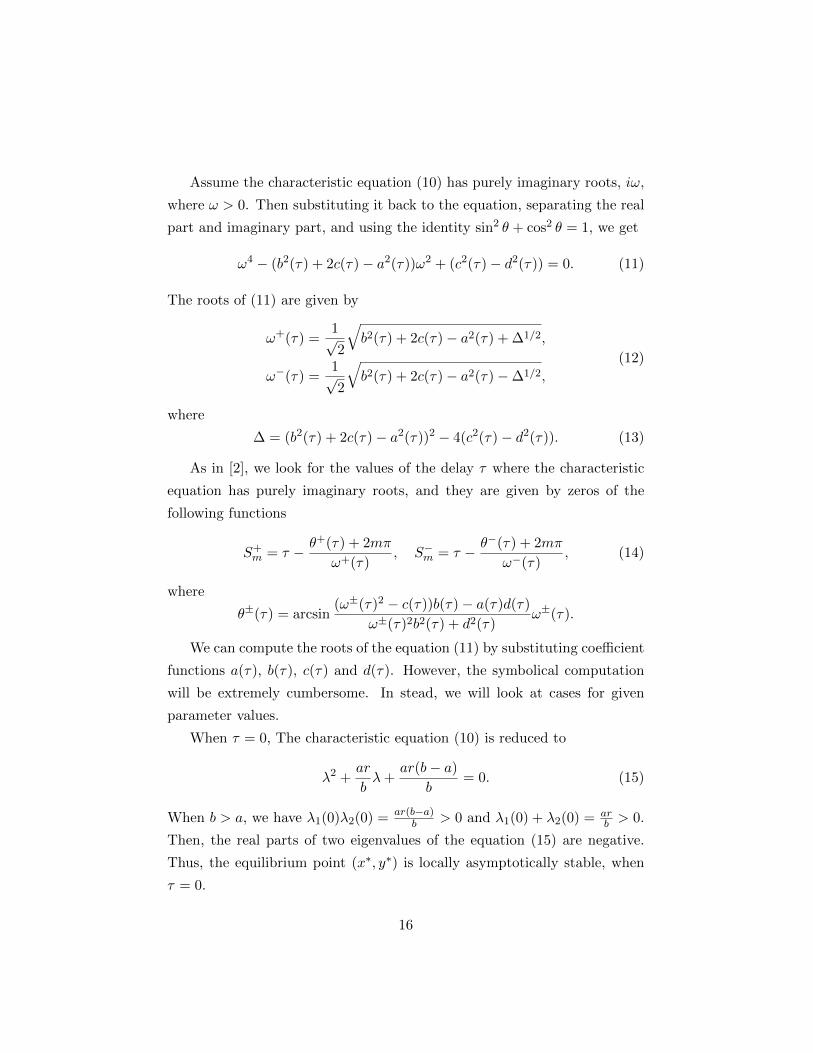
Assume the characteristic equation (10) has purely imaginary roots, iω,
where ω > 0. Then substituting it back to the equation, separating the real
part and imaginary part, and using the identity sin2 θ + cos2 θ = 1, we get
ω4 − (b2(τ) + 2c(τ)− a2(τ))ω2 + (c2(τ)− d2(τ)) = 0. (11)
The roots of (11) are given by
ω+(τ) =1√2
√b2(τ) + 2c(τ)− a2(τ) + ∆1/2,
ω−(τ) =1√2
√b2(τ) + 2c(τ)− a2(τ)−∆1/2,
(12)
where
∆ = (b2(τ) + 2c(τ)− a2(τ))2 − 4(c2(τ)− d2(τ)). (13)
As in [2], we look for the values of the delay τ where the characteristic
equation has purely imaginary roots, and they are given by zeros of the
following functions
S+m = τ − θ+(τ) + 2mπ
ω+(τ), S−m = τ − θ−(τ) + 2mπ
ω−(τ), (14)
where
θ±(τ) = arcsin(ω±(τ)2 − c(τ))b(τ)− a(τ)d(τ)
ω±(τ)2b2(τ) + d2(τ)ω±(τ).
We can compute the roots of the equation (11) by substituting coefficient
functions a(τ), b(τ), c(τ) and d(τ). However, the symbolical computation
will be extremely cumbersome. In stead, we will look at cases for given
parameter values.
When τ = 0, The characteristic equation (10) is reduced to
λ2 +ar
bλ+
ar(b− a)
b= 0. (15)
When b > a, we have λ1(0)λ2(0) = ar(b−a)b > 0 and λ1(0) + λ2(0) = ar
b > 0.
Then, the real parts of two eigenvalues of the equation (15) are negative.
Thus, the equilibrium point (x∗, y∗) is locally asymptotically stable, when
τ = 0.
16

Taking b = 1, a = 0.2, n = 0.01, these coefficients become,
a(τ) =0.2− 0.8r + r(0.4 + 0.2r)e
τ100
1 + r, b(τ) =
re−τ
100 − (0.2 + 0.4r)
1 + r,
c(τ) =−0.2r + 0.2r(0.4 + 0.2r)e
τ100
1 + r, d(τ) =
0.2re−τ
100 + r(0.08 + 0.12r)
1 + r.
When r > 0.5, ∆ > 0 for τ ≥ 0. If r = 1.5, (ω+)2 > 0 for 0 ≤ τ ≤ 79.2,
while (ω−)2 < 0 for all feasible τ . Thus, we only consider S+m. In the
feasible range, S+0 (τ) has one zero, µ0,1 ≈ 1.98. S+
1 (τ) has two zeros, the
bigger one is µ2,2 ≈ 77. Therefore, there exist stability switches start from
this equilibrium solution (ab ,1−a
b
1+ br
). Figure (3) shows plots of functions S+m.
0 10 20 30 40 50 60 70 80−150
−100
−50
0
50
100
tau
S
S+0
S+1
Figure 3: Plots of the functions S+m(τ), m = 0, 1. The parameter values
are b = 1, a = 0.2, n = 0.01 and r = 1.5. Since the scale in the picture is
relatively big, the intersection point of the function S+0 (τ) and τ = 0 is not
clearly shown. However, the function S+0 (τ) has a root, µ0,1 ≈ 1.98. The
function S+1 (τ) has two roots, µ2,1 ≈ 14 and µ2,2 ≈ 77.
The interior equilibrium is the function of the delay parameter τ , (x∗(τ), y∗(τ)).
The interior equilibrium solution is locally asymptotical stable when 0 ≤ τ <
17

µ0,1. The interior equilibrium solution is unstable when µ0,1 < τ < µ2,2, and
is unstable when τ > µ2,2. The pictures in the right columns of the Figures
(4)-(8) show these cases with various values of the delay parameter τ .
Comparing the stability of the equilibrium solutions (1, 0) and (x∗(τ), y∗(τ)),
we observe that in some intervals of the delay parameter τ one equilibrium
is stable while the other is unstable as shown in Figures (4)-(8). We obtain a
rough picture of the dynamics of the model (4) as follows. The equilibrium
(0, 0) is always unstable. Without the delay, the equilibrium (1, 0) is un-
stable while the equilibrium (ab ,1−a
b
1+ br
) is locally asymptotical stable. When
the delay parameter τ is small, the interior equilibrium (x∗(τ), y∗(τ)) is still
locally asymptotical stable and (1, 0) is unstable. When the delay parameter
τ is becoming greater, the equilibrium (x∗(τ), y∗(τ)) is unstable. When τ is
even bigger, the equilibrium (x∗(τ), y∗(τ)) is stable again.
5 Discussion
The parameter b represents the non-dimensionalized infectivity of the virus
while a represents the death rate of infected tumor cells. The theorem (4.2)
states how these two parameters effect the virotherapy. When b < a, the
equilibrium solution x = 1 and y = 0 is globally stable for any time delay.
The tumor reaches its maximum size, and the therapy fails. On the other
hand, from the viewpoint of epidemiology modeling, the condition b < a
implies the basic reproduction number
R0 =β
ae−nτ =
b
aKe−nτ =
b
a
1
Ke−nτ < 1,
since the maximum size of the tumor is obviously greater than 1 and e−nτ ≤1. Therefore, the infection can not spread out, and the infection free equi-
librium is stable.
The relative sizes of the parameter a and b are dominant factors in
virotherapy. In animal experiments, the viruses have high possibility to kill
the tumor if the virus is more infectious. The virus has a high infectivity
if it is more infectious to tumor cells. There are various genetic methods
18
0 100 200 300 400 500 600 700 800 900 10000
0.1
0.2
0.3
0.4
0.5
0.6
0.7
0.8
0.9
1
time t
x,y
The infection−free equilibrium
uninfected tumor cell x
infected tumor cell y
tau = 1, history x = 0.91 and y = 0.08
(a)
0 100 200 300 400 500 600 700 800 900 10000.15
0.2
0.25
0.3
0.35
0.4
0.45
0.5
0.55The interior equilibrium
time tx,
y
uninfected tumor cell x
infected tumor cell y
tau = 1, the history x = 0.29, y = 0.41
(b)
0 100 200 300 400 500 600 700 800 900 10000
0.1
0.2
0.3
0.4
0.5
0.6
0.7
0.8
0.9
1The infection free equilibrium
time t
x, y
uninfected tumor cell x
infected tumor cell y
tau = 2, the history x = 091, y = 0.08
(c)
0 100 200 300 400 500 600 700 800 900 10000.1
0.15
0.2
0.25
0.3
0.35
0.4
0.45
0.5
0.55
0.6
time t
x, y
The interior equilibrium
ununfected tumor cell x
infected tumor cell y
tau = 2, the history x = 0.29, y = 0.41
(d)
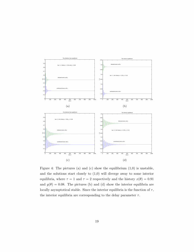
Figure 4: The pictures (a) and (c) show the equilibrium (1,0) is unstable,
and the solutions start closely to (1,0) will diverge away to some interior
equilibria, where τ = 1 and τ = 2 respectively and the history x(θ) = 0.91
and y(θ) = 0.08. The pictures (b) and (d) show the interior equilibria are
locally asymptotical stable. Since the interior equilibria is the function of τ ,
the interior equilibria are corresponding to the delay parameter τ .
19

0 100 200 300 400 500 600 700 800 900 10000
0.1
0.2
0.3
0.4
0.5
0.6
0.7
0.8
0.9
1The infection free equilibrium
time t
x, y
uninfected tumor cell x
infected tumor cell y
tau = 3, the history x = 0.95, y = 0.07
(a)
0 100 200 300 400 500 600 700 800 900 10000
0.1
0.2
0.3
0.4
0.5
0.6
0.7The interior equilibrium, tau = 3
time t
x, y
uninfected tumor cell x
infected tumor cell y
(b)
0 100 200 300 400 500 600 700 800 900 10000
0.1
0.2
0.3
0.4
0.5
0.6
0.7
0.8
0.9
1The infection free equilibrium, tau = 10
time t
x, y
x
y
(c)
0 100 200 300 400 500 600 700 800 900 10000
0.1
0.2
0.3
0.4
0.5
0.6
0.7
0.8
0.9The interior equilibrium, tau = 10
time t
x, y
x
y
(d)
Figure 5: The pictures (a) and (c) show some solutions which start closely to
(1,0), and they are periodic solutions, where τ = 3 and τ = 10 respectively,
and the history x(θ) = 0.95 and y(θ) = 0.07. The pictures (b) and (d) show
some solutions with the history x(θ) = 0.29 and y(θ) = 0.41, and τ = 3 and
τ = 10 respectively.
20

0 100 200 300 400 500 600 700 800 900 10000
0.1
0.2
0.3
0.4
0.5
0.6
0.7
0.8
0.9
1The infection free equilibrium, tau = 20
x, y
time t
x
y
(a)
0 100 200 300 400 500 600 700 800 900 10000
0.1
0.2
0.3
0.4
0.5
0.6
0.7
0.8The interior equilibrium, tau = 20
time t
x, y
x
y
(b)
0 100 200 300 400 500 600 700 800 900 10000
0.1
0.2
0.3
0.4
0.5
0.6
0.7
0.8
0.9
1The infection free equilibrium, tau = 30
time t
x, y
x
y
(c)
0 100 200 300 400 500 600 700 800 900 10000
0.1
0.2
0.3
0.4
0.5
0.6
0.7
0.8The interior equilibrium, tau = 30
time t
x, y
x
y
(d)
Figure 6: The pictures (a) and (c) show some solutions which start closely to
(1,0), and they are periodic solutions, where τ = 20 and τ = 30 respectively,
and the history x(θ) = 0.95 and y(θ) = 0.07. The pictures (b) and (d) show
some solutions with the history x(θ) = 0.28 and y(θ) = 0.45, and τ = 20
and τ = 30 respectively.
21
0 100 200 300 400 500 600 700 800 900 10000
0.1
0.2
0.3
0.4
0.5
0.6
0.7
0.8
0.9
1The infection free equilibrium
time t
x, y
y
x
tau = 40, the history x = 0.95, y = 0.07
(a)
0 100 200 300 400 500 600 700 800 900 10000.1
0.15
0.2
0.25
0.3
0.35
0.4
0.45
0.5
0.55
0.6
time t
x, y
The interior equilibrium, tau = 40
y
x
(b)
0 100 200 300 400 500 600 700 800 900 10000
0.1
0.2
0.3
0.4
0.5
0.6
0.7
0.8
0.9
1
time t
x, y
The infection free equilibrium
x
y
tau = 50, the history x = 0.95 and y = 0.07
(c)
0 200 400 600 800 1000 1200 1400 1600 1800 20000.2
0.25
0.3
0.35
0.4
0.45
0.5The interior equilibrium
time t
x, y
tau = 50, the history x = 0.23 and y = 0.45
x
y
(d)
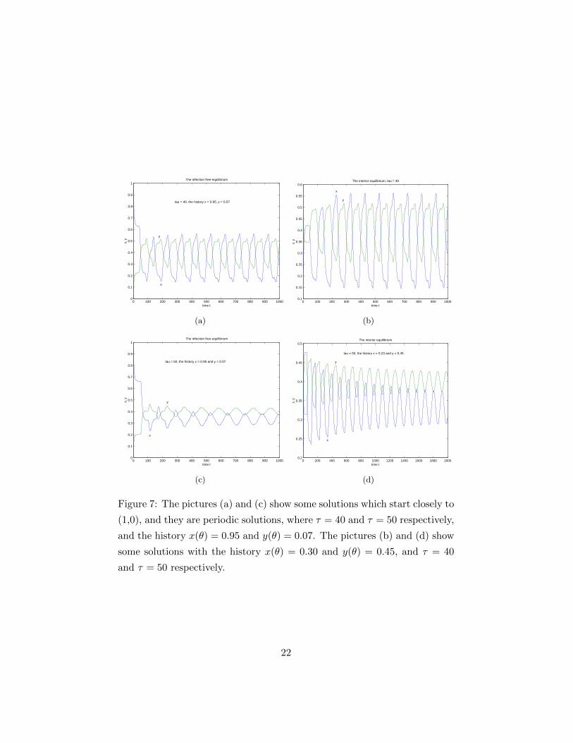
Figure 7: The pictures (a) and (c) show some solutions which start closely to
(1,0), and they are periodic solutions, where τ = 40 and τ = 50 respectively,
and the history x(θ) = 0.95 and y(θ) = 0.07. The pictures (b) and (d) show
some solutions with the history x(θ) = 0.30 and y(θ) = 0.45, and τ = 40
and τ = 50 respectively.
22
0 100 200 300 400 500 600 700 800 900 10000
0.1
0.2
0.3
0.4
0.5
0.6
0.7
0.8
0.9
1The infection free equilibrium
time t
x, y
x
y
tau = 60, the history x = 0.95 and y = 0.07
(a)
0 100 200 300 400 500 600 700 800 900 10000.2
0.25
0.3
0.35
0.4
0.45
0.5
0.55The interior equilibrium
time tx,
y
x
y
tau = 60, the history x = 0.23 and y = 0.45
(b)
0 100 200 300 400 500 600 700 800 900 10000
0.1
0.2
0.3
0.4
0.5
0.6
0.7
0.8
0.9
1
time t
x, y
The infection free equilibrium
x
y
tau = 70, the history x = 0.95 and y = 0.1
(c)
0 100 200 300 400 500 600 700 800 900 10000.2
0.25
0.3
0.35
0.4
0.45
0.5
0.55
0.6
0.65The interior equilibrium
time t
x, y
x
y
tau = 70, the history x = 0.23, y = 0.45
(d)
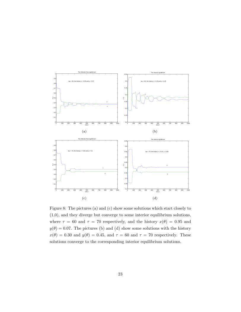
Figure 8: The pictures (a) and (c) show some solutions which start closely to
(1,0), and they diverge but converge to some interior equilibrium solutions,
where τ = 60 and τ = 70 respectively, and the history x(θ) = 0.95 and
y(θ) = 0.07. The pictures (b) and (d) show some solutions with the history
x(θ) = 0.30 and y(θ) = 0.45, and τ = 60 and τ = 70 respectively. These
solutions converge to the corresponding interior equilibrium solutions.
23

that can be applied to modify the genomes of viruses so that the viruses
have high infectivity [3]. Therefore, the virus with a low infectivity b that
is smaller than the death rate of infected tumor cells can not be used to
eradicate the tumor. However, when the infectivity is greater than the
death rate of infected tumor cells b > a, the dynamics of virotherapy is
much more complicated, where the intracellular viral life-cycle comes to
play an important role.
Theoretically, when the infectivity b is greater than the death rate a of
infected tumor cells, the viruses can not eradicate the tumor if the period
of the intracellular viral life-cycle is ignored. As the equation (15) shown,
it has two eigenvalues with negative real parts. The interior equilibrium
solution (x∗, y∗) is locally asymptotical stable. In the feasible domain Σ of
the model, there is a large port of the domain which is in the attractive
range of this equilibrium point. That means, the tumor cells and infected
tumor cells coexist, and the viruses can not eradicate the tumor. We also
can see this point from the expression of the basic reproduction number
R0 = βa e−nτ = b
aK e−nτ = b
a1K . The condition b > a alone can not guarantee
R0 > 1. Even b is big enough such that R0 > 1, it only makes the interior
equilibrium solution is locally asymptotical stable.
When the period of the intracellular viral life-cycle is incorporated into
the model, but with the period modeled as the delay parameter, the tumor
cells still can not be completely eradicated. When the delay parameter
has a small value, tumor cells and infected tumor cells coexist, and the
coexisting equilibrium solution is still locally asymptotical stable. If the
viruses have a longer period of the intracellular viral life-cycle, the stability of
the coexisting equilibrium solution will be broken. This creates a possibility
of killing the tumor. Since the interior equilibrium solution is unstable in this
case, the tumor cell population and the infected tumor cell population will
not rest on a fixed level. Instead, they will periodically change over time or
diverge away. The virotherapy seeks to decrease the tumor cell amount even
it can not eradicate the tumor. The success of the therapy is determined
by detectability of the tumor cells. Thus, it is considered as a successful
24
therapy if the tumor cell amount is below a detective level. In our case, it is
possible that other parameters like the survival probability function can be
chosen so that the periodic solution with lower tumor component. We then
can obtain a good result of the virotherapy.
In many clinical and theoretical studies of virotherapy, the periodic phe-
nomena were observed. When the value of the delay parameter is in this
middle range, our model has stable periodic solutions. Thus, the intracel-
lular viral life-cycle can explain periodic phenomena observed in [5, 14, 16]
and other work.
However, when the intracellular viral life-cycle is too long, the interior
equilibrium solution becomes locally asymptotical stable again. In this situ-
ation, the tumor cell component has even big quantity as ab enτ is increasing
function of τ . This is undesirable. When the intracellular viral life-cycle
is even longer, the virotherapy totally fails since the interior equilibrium
solution will be lost and there are only two equilibria (0, 0) and (1, 0).
Overall, a clinic implication is that the period of the intracellular vi-
ral life-cycle should also be modified when a type of a virus is modified
for virotherapy, so that the period of the intracellular viral life-cycle is in
a suitable range which can break the stability of the interior equilibrium
solution.
Acknowledgment
The authors would like to thank the reviewer for helpful suggestions that
lead to better model presentation. J.P. Tian gratefully acknowledges the
support of a start-up fund at the College of William and Mary. Y. Kuang
gratefully acknowledges support from National Science Foundation grants
DMS-0436341 and DMS-0920744. H. Yang gratefully acknowledges support
in part by the National Science Foundation of China under grant 10961025.
25

References
[1] Z. Bajzer, T. Carr, K. Josic, S.J. Russel, D. Dingli, Modeling of cancer
virotherapy with recombinant measles viruses, J. Theoretical Biology,
252(2008), 109-122.
[2] E. Beretta, Y. Kuang, Geometric stability switch criteria in delay dif-
ferential systems with delay dependent parameters, SIAM J. Anal. Vol.
33 (2002), No. 5, pp. 1144-1165.
[3] E.A. Chiocca, Oncolytic viruses, Nature reviews, Cancer. Vol. 2(2002),
no. 12: 938-50.
[4] B.R. Dix, S.J. OCarroll, C.J. Myers, S.J. Edwards, A.W. Baithwaite,
Efficient induction of cell death by adenoviruses requires binding of E1B
and p53, Cancer Res. 60(2000), 26662672.
[5] A. Friedman, J.P. Tian, G. Fulci, E.A. Chiocca, J. Wang, Glioma vi-
rotherapy: effects of innate immune suppression and increased viral
replication capacity, Cancer Research, Vol.66 (2006), 2314-2319.
[6] A.R. Hall, B.R. Dix, S.J. OCarroll, A.W. Braithwaite, p53-dependent
cell death/apoptosis is required for a productive adenovirus infection,
Nature Med. 4(1998), 10681072.
[7] J.N. Harada, A.J. Berk, p53-independent and -dependent requirements
for E1B-55k in adenovirus type 5 replication, J. Virol. 73(1999),
53335344
[8] E. Kelly and S.J. Russell, History of Oncolytic Viruses: Genesis to
Genetic Engineering, Molecular Therapy, Molecular Therapy, 15(2007),
no. 4, 651659.
[9] K.A. Parato, D. Senger, A.J. Forsyth and J.C. Bell, Recent progress
in the battle between oncolytic viruses and tumours, Nature reviews,
Cancer, Vol. 5(2005), 965-976.
26

[10] H. Kambara, H. Okano, E.A. Chiocca, Y. Saeki, An oncolytic HSV-1
mutant expressing ICP34.5 under control of a nestin promoter increases
survival of animals even when symptomatic from a brain tumor, Cancer
Res. 65(2005), no. 7, 2832-2839.
[11] N.L. Komarova, D. Wodarz, ODE models for oncolytic virus dynamics,
J Theor Biol. 263(2010), no. 4, 530-43.
[12] T.-C. Liu and D. Kirn, Systemic efficacy with oncolytic virus ther-
apeutics: clinical proof-of-concept and future directions, Cancer Res.
67(2007): 429-432.
[13] M. Ramachandra, et al. Re-engineering adenovirus regulatory path-
ways to enhance oncolytic specificity and efficacy, Nature Biotechnol.
19(2001), 10351041.
[14] J.P. Tian, The replicability of oncolytic virus: defining conditions in
tumor virotherapy, Math. Biosci. Eng. 8(2011), 841-860.
[15] Y. Tao, Q. Quo, The competitive dynamics between tumor cells, a
replication-competent virus and an immune response, J. Math. Biol.
51(1) (2005), 37-78.
[16] J.T. Wu, H.M. Byrne, D.H. Kirn, L.M. Wein, Modeling and analysis
of a virus that replicates selectively in tumor cells, Bull. Math. Biol. 63
(2001) (4), 731-768.
[17] L.M. Wein, J.T. Wu, D.H. Kirn, Validation and analysis of a math-
ematical model of a replication-competent oncolytic virus for cancer
treatment: implications for virus design and delivery, Cancer Res.
63(6)(2003), 1317-1324.
[18] D. Wodarz, Viruses as antitumor weapons: defining conditions for tu-
mor remission, Cancer Res. 61(2001), 3501-3507.
27

[19] D. Wodarz, N.L. Komarova, Towards predictive computational models
of oncolytic virus therapy: basis for experimental validation and model
selection, PloS ONE, Vol.4 (2009), (1), e4271.
[20] A.S. Novozhilov, F.S. Berezovskaya, E.V. Koonin, G.P. Karev, Math-
ematical modeling of tumor therapy with oncolytic viruses: Regimes
with complete tumor elimination within the framework of deterministic
models, Biology Direct, 1:6 (2006), 1-18.
28
Recommended


![George ]DPSN Hyang Eom's · 2017. 3. 11. · PRIMARY POINT forhelp.ButWiSahnwasatoughteacher.Hesaid,"Icould tellyoumyexperienceofpracticebutitwouldn'thelpyouin the slightest and in](https://img.dokumen.tips/doc/110x75/5fd396b95dcee236e336cb8b/george-dpsn-hyang-eoms-2017-3-11-primary-point-forhelpbutwisahnwasatoughteacherhesaidicould.jpg)