International Trade and the Gender Wage Gap:
New Evidence from India’s Manufacturing Sector
Nidhiya Menon, Brandeis University
Yana van der Meulen Rodgers, Rutgers University
September 2008
Corresponding author: Yana van der Meulen Rodgers, Women’s and Gender Studies
Department, Rutgers University, New Brunswick, NJ 08901. Tel 732-932-1151 x641, fax 732-
932-1335, email [email protected]. Contact information for Nidhiya Menon: Department
of Economics & IBS, MS 021, Brandeis University, Waltham, MA 02454-9110. Tel 781-736-
2230, fax 781-736-2269, email [email protected].
2
International Trade and the Gender Wage Gap:
New Evidence from India’s Manufacturing Sector
Abstract: This study examines how increasing competitive forces from India’s trade
liberalization have affected women’s relative wages and employment. Neoclassical theory
implies that costly discrimination against female workers should diminish over time with
increased competition. We incorporate this idea into a theoretical model of competition and
industry concentration and test the model using repeated cross sections of India’s NSSO
household survey data merged with trade and production data from 1983 to 2004. Estimates from
OLS and Fixed Effects regressions at the industry level indicate that increasing openness to trade
is associated with larger wage gaps in India’s concentrated manufacturing industries.
Keywords: Trade liberalization, Gender wage gap, India, Discrimination, Asia, Competition

3
Author Acknowledgments
We thank Narayanan Subramanian, Elizabeth Brainerd, Puja Dutta, Ira Gang, Subhashis
Gangopadhyay, Rachel McCulloch, Nina Pavcnik, Eric Edmonds, Bernard Hoekman, Susan
Razzaz, and participants in the University of Pennsylvania Family Macro workshop and the
UNDP-Fordham University gender and poverty series for their helpful suggestions. Thanks also
to three anonymous referees whose comments have greatly improved the paper. Funding from
Brandeis University’s Theodore and Jane Norman research grant is gratefully acknowledged.
The usual caveat applies.

1
1. INTRODUCTION
Precipitated by a balance of payments crisis, India has adopted several waves of far-
reaching trade reforms since 1991. The reforms have included sharp reductions in the number of
goods subject to licensing and other non-tariff barriers, reductions in export restrictions, and
tariff cuts across all industries. These changes raises an interesting question as to how the new
wave of competitive forces and the growing pressure for employers to cut costs have affected the
wages of male and female workers in India’s manufacturing sector. With less government
protection and with increased exposure to competition from abroad, employment and pay
patterns in manufacturing changed markedly following the liberalization. Yet manufacturing
industries experienced quite a bit of variation in the timing and extent of tariff cuts during and
after the 1991 reforms. These differential rates in trade liberalization across industries provide an
excellent opportunity for examining the impact of increasing exposure to international trade on
gender wage differentials.
Neoclassical theory of labor market discrimination implies that increased competition
from international trade will reduce the wage gap. In a market economy where discrimination is
costly, employers are less able to discriminate against women as competitive forces drive down
profit margins (Becker 1971). We incorporate this idea into a theoretical model of competition
and industry concentration in which the impact of international trade on the gender wage gap
depends on changes in market characteristics and a parameter which represents the wage
premium paid to male workers. Our theoretical model introduces elements of discriminatory
firm behavior into a competitive market framework to show that the implied outcome of a
reduction in the wage gap does not necessarily hold. We then test the theory by estimating the
impact of the trade reforms on gender wage differentials using five cross sections of household

2
survey data from the National Sample Survey Organization between 1983 and 2004. We
aggregate these data to the industry level and merge the data with several other industry-level
data sets for international trade, output, and industry structure.
The empirics examine the relationship between the male-female residual wage gap and
variations across time and industry in exposure to international trade competition. Our strategy
centers on comparing the effects of international trade in India’s more-concentrated
manufacturing industries, where firms enjoyed rents and could afford the costs associated with
discrimination, with trade effects in India’s less-concentrated manufacturing industries, where
firms experienced greater domestic competition and were less able to discriminate. Following
Black and Brainerd (2004), this strategy is adopted since the aim here is to measure the effect of
increased international trade (resulting from trade liberalization) on the gender wage gap.
Industries in the less concentrated (competitive) sector are subject to competition from other
industries in the same sector, and are perhaps also subject to competition from overseas as a
consequence of increased openness to trade. Suppose there was an increase in the gender wage
gap in the less concentrated sector. Because industries in this sector are exposed to other forces
in addition to those of increased international trade, it would not be clear what part of the
increase in the gender wage gap was due to trade liberalization and what part was due to
competition from domestic forces. Since industries in the concentrated sector are relatively
insulated from domestic competition, any change in the gender pay differential in this sector
could be attributed more unambiguously to international trade. Thus as in Black and Brainerd
(2004), we adopt a difference-in-difference-in-difference approach (which exploits sources of
variation across time, industry-level domestic concentration, and industry-level openness to
trade) to measure the effect of international trade on the gender wage gap, where industries in the

3
less concentrated sector are used as a control for changes in the relative pay differential that may
not be due to increased exposure to trade (for example, changes in the educational attainment or
labor force attachment of female workers).
The impact of increased competitiveness from international trade on women’s relative
pay remains an empirical issue. Relatively few studies have gone beyond descriptive analyses of
changes in women’s relative wages in periods of increasing trade openness and growing
competition.1 The limited number of studies that do employ econometric techniques to identify
the impact of competition and international trade on gender wage gaps have found conflicting
results. In particular, Hellerstein, Neumark, and Troske (2002), find little evidence that more
discriminatory employers with market power are punished over time through buy-outs or lower
growth. Berik et al. (2004) find evidence that increasing trade openness is associated with higher
residual wage gaps between men and women in two East Asian economies, a sign the authors
interpret as increased wage discrimination.2 Yet Black and Brainerd (2004) reach the opposite
conclusion for the United States: relatively concentrated manufacturing industries that were
exposed to more competition from imports experienced shrinking residual wage gaps. Similarly
in Mexico, trade-induced competition in product markets is associated with lower gender
earnings differentials (Hazarika and Otero (2004). Cross-country studies have found mixed
evidence. Using data for more than 80 lower- and higher-income economies, Oostendorp (2004)
shows that increased trade is associated with reduced wage gaps. However, the opposite result is
obtained in the case of skilled workers in lower-income economies.
With our focus on India’s extensive trade policy reforms, this study also contributes to a
lively debate in the literature on the net social benefits of India’s trade liberalization. For
example, evidence from a difference-in-difference approach in Topalova (2005) indicates that in
4
districts that were more exposed to trade liberalization, both the incidence and depth of poverty
decreased by less than the reductions observed in other districts that had fewer industries
exposed to trade liberalization. India’s trade liberalization also appears to have had negative
impacts on child well-being. Findings in Edmonds et al. (2005) suggest that adjustment costs
associated with trade liberalization were responsible for smaller declines in child labor and
smaller improvements in school attendance in districts exposed to tariff cuts, compared to
districts less exposed to the tariff reductions.3 Trade liberalization also had differential effects on
male and female employment in India. According to Bhaumik (2003), the growth in the
workforce share classified as casual accelerated after 1993 as a result of the economic
liberalization policies, with larger increases for female workers compared to their male
counterparts in both rural and urban areas. Unskilled workers also did not fare well under trade
liberalization, with findings in Dutta (2007) showing that tariff cuts had an adverse effect on the
relative wages of unskilled workers and on overall wage inequality. Furthermore, disparities in
the material standard of living have persisted among Indian women of different castes during the
early years of economic liberalization, despite improvements in educational attainment
(Deshpande 2007).
However, not all studies have found negative social impacts for India. In particular,
Chamarbagwala (2006) examines labor market supply and demand shifts associated with India’s
trade liberalization and domestic economic reforms and finds that skill upgrading within India’s
industries led to large demand increases for skilled labor and the creation of new white collar
jobs, especially in the service sector.4 Moreover, rapid economic growth in the 1990s following
India’s liberalization is associated with improvements in short-term and longer-term indicators of
children’s nutritional status, especially for boys (Tarozzi and Mahajan 2007). Adding to this

5
debate, we ask how the competitive market forces associated with India’s trade policy reforms
may have affected discriminatory pay practices in the manufacturing sector. We find that
increasing openness to trade is associated with a widening in the wage gap in India’s
concentrated manufacturing industries.
2. THEORETICAL MODEL: TRADE COMPETITION, MARKET POWER, AND
DISCRIMINATION
In a neoclassical framework, discrimination is costly to employers and will not persist in
a competitive market environment (Becker 1971). This hypothesis can be restated in an open
economy context, whereby firms operating in industries that face international competition will
experience greater pressure to cut costs, including costs associated with discrimination. In the
longer term, discrimination is then expected to lessen in industries that are more open to trade.
One can hypothesize that firms in concentrated industries face less competition from other
domestic firms, and therefore experience less domestic pressure to cut costs (Borjas and Ramey
1995). If discrimination is costly, then we would expect any observed reduction in wage
discrimination against female workers in concentrated industries to be caused by the competitive
forces from international trade rather than other domestic firms (Black and Brainerd 2004). In
the exposition that follows, Borjas and Ramey (1995), which, in turn, is based on Abowd and
Lemieux (1991), is used as the foundation to obtain an expression for equilibrium wages
received by workers employed in the concentrated sector. We then model the distribution of
equilibrium wages between male and female employees in the concentrated sector by building on
Becker (1971).
Before discussing the mechanics of the model, it is useful to provide a brief description
of what the model accomplishes. Neoclassical theory based on Becker (1971) implies that an

6
increase in competition associated with trade should reduce the male-female wage gap. Non-
neoclassical theory, as developed in Darity and Williams (1985) and Williams (1987), implies
that an increase in trade can actually increase gender wage gaps in countries where female
workers may have lower bargaining power and where women are segregated into lower-paying,
lower-status jobs. The model we develop below is a combination of these effects.
Following Borjas and Ramey (1995) and Abowd and Lemieux (1991), the domestic
economy consists of two sectors, the competitive sector (sector 0) and the concentrated sector
(sector 1). The competitive sector produces a consumption good 0y , and the concentrated sector
produces a consumption good 1y . In other sections of our study, we refer to the competitive
sector as the less-concentrated sector. Development of the competitive sector follows Borjas and
Ramey (1995) and is not discussed in detail here. Similar to their formulation of the
concentrated sector, sector 1 in our study is composed of n firms, each of whom behaves as a
Cournot oligopolist. We begin by considering an inverse demand curve that relates price of good
1y relative to price of 0y ( 1p ) to the total demand for good 1y . 5 This inverse demand curve is
01 β=p - 11 yβ 0, 10 >ββ (1)
Total output of the concentrated sector in the domestic economy ( 1y ) is composed of the
sum of the output of firm i , iy1 , the output of the other )1( −n firms each of whom produces '1y ,
and v , which is the volume of net trade in good 1. Like Borjas and Ramey (1995), we assume
that v is exogenous. This is necessary to ensure an unbiased measure of the effect of trade on
relative gender pay differentials. Re-writing (1), the inverse demand curve now is
01 β=p - ))1(( '111 vyny i +−+β (2)
7
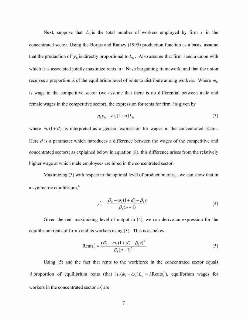
Next, suppose that iL1 is the total number of workers employed by firm i in the
concentrated sector. Using the Borjas and Ramey (1995) production function as a basis, assume
that the production of iy1 is directly proportional to iL1 . Also assume that firm i and a union with
which it is associated jointly maximize rents in a Nash bargaining framework, and that the union
receives a proportion λ of the equilibrium level of rents to distribute among workers. Where 0ω
is wage in the competitive sector (we assume that there is no differential between male and
female wages in the competitive sector), the expression for rents for firm i is given by
ii Ldyp 1011 )1( +−ω (3)
where )1(0 d+ω is interpreted as a general expression for wages in the concentrated sector.
Here d is a parameter which introduces a difference between the wages of the competitive and
concentrated sectors; as explained below in equation (8), this difference arises from the relatively
higher wage at which male employees are hired in the concentrated sector.
Maximizing (3) with respect to the optimal level of production of iy1 , we can show that in
a symmetric equilibrium,6
)1()1(
1
100*1 +
−+−=
nvd
y i ββωβ
(4)
Given the rent maximizing level of output in (4), we can derive an expression for the
equilibrium rents of firm i and its workers using (3). This is as below
21
2100*
)1())1((
Rents+
−+−=
nvd
i ββωβ
(5)
Using (5) and the fact that rents to the workforce in the concentrated sector equals
λ proportion of equilibrium rents (that is, *101 Rents)( iiL λωω =− ), equilibrium wages for
workers in the concentrated sector *1ω are

8
)1())1(( 100
0*1 +
−+−+=
nvd βωβ
λωω (6)
Equation (6) highlights two things - the first is that wages in the concentrated sector
differ from wages in the competitive sector by a mark-up which is often positive. This is the
case in the five years of NSSO data that we consider, where the average real wage of workers in
the concentrated sector is higher than that of workers in the less-concentrated sector. The second
point is that since average real wages in the concentrated sector are higher, women may still
want to be employed there despite receiving relatively lower pay.
Next, we model the distribution of wages between male and female workers in the
concentrated sector. To derive a measure for the gender wage gap in this sector, we postulate
that the equilibrium wage in (6) is the weighted average of the wages paid to male and female
workers, where weights are the shares of male and female workers. That is,
fmmm ss 11*1 )1( ωωω −+= (7)
where ms is the share of males among all workers in the concentrated sector, m1ω represents
wages to males, and f1ω represents wages to females in this sector. From Becker (1971), a wage
gap exists in the concentrated sector as male workers are employed by firm i at a relatively
higher wage, as follows
)1(11 dfm += ωω (8)
where d is the parameter that represents the wage premium for male employees in the
concentrated sector.7 Deriving an expression for *1ω in terms of the female wage f
1ω (using (8))
and substituting this in (7), we can show that
*1
1001 )1(
)1()1
))1(((
)1()1(*
ωβωβ
λωω mo
mm
dsd
nvd
dsd
++
=+
−+−+
++
= (9)

9
and
*1
1001 )1(
1)1
))1(((
)1(1*
ωβωβ
λωω mo
mf
dsnvd
ds +=
+−+−
++
= (10)
What determines d? In the context of our study, we formulate that d is positively
influenced by the exogenous net trade in good 1, measured by v . Why might d increase with
v ? Plausible reasons include the fact that with trade, rents in the concentrated sector fall. This
assertion is supported by evidence in Krishna and Mitra (1998) showing that trade liberalization
has resulted in higher levels of competition within the Indian economy, as measured by
reductions in price markups over marginal cost. If firms in the concentrated sector discriminate
against women, they may want to maintain male wages at the expense of female wages. With
smaller rents, this means that female wages fall more, that is, d increases.
An increase in d with trade is also consistent with the theoretical model developed in
Rosen (2003). Rosen extends the Becker argument in a framework that includes search frictions
in the labor market as well as wages set by bargaining. The discrimination coefficient is a firm-
specific disutility associated with hiring female workers, and this coefficient affects firm profits
through wages and hiring. Although discriminatory firms employ male and female workers,
firms with high discrimination coefficients are more selective in their hiring decisions for female
workers than male workers, causing them to hire fewer than the optimal number of female
workers. At the same time, discriminatory firms pay their female workers relatively low wages,
which contributes to a total wage bill that is less than the wage bill of non-discriminatory firms.
Because the positive profit impact from a lower wage bill dominates the negative profit impact
from the suboptimal hiring decisions, discriminatory firms are more profitable. In this
framework, competitive market forces drive out non-discriminatory firms instead of
discriminatory firms. Placing our study in the context of Rosen (2003), the average value of d

10
(across firms) may rise with international trade since firms with lower d are less profitable and so
exit the market. We model the positive link between d and v as:
vd 10 αα += ; 01 >α (11)
Note that (11) implies that v determines d, which, in turn, influences equilibrium male
and female wages in the concentrated sector as in equations (9) and (10). Econometrically,
equation (11) may be thought of as a reduced form equation.
We conclude our theory by definingψ , the relative difference between male and female
wages in the concentrated sector. Thus,
*
*
*
**
1
1
1
11 1m
f
m
fm
ω
ω
ω
ωωψ −=
−= (12)
Substituting from (9), (10), and (11) above,
)1()(
)1( 10
10
vv
dd
αααα
ψ++
+=
+= (13)
Soψ , the gender wage differential in the concentrated sector, is a function of the parameter d .
To study the effect of an increase in trade on the gender wage differential in the concentrated
sector, we are interested in the following derivative of (13):
0)1( 2
10
1 >++
=∂∂
vv αααψ (14)
From (14), the relative pay differential in the concentrated sector increases with trade. These
theoretical implications are tested in the empirics that follow.
3. DATA DESCRIPTION
To explore the labor market impacts of trade policy reforms, we use five cross sections of
household survey data collected by the National Sample Survey Organization (NSSO). The data
include the years 1983 (38th round), 1987-1988 (43rd round), 1993-1994 (50th round), 1999-2000

11
(55th round), and 2004 (60th round), providing us with data coverage before, during, and after the
trade liberalization. For each round, we utilize the Employment and Unemployment module -
Household Schedule 10. To construct our labor force sample, we retain all regular wage
employees of prime working age (ages 15-60) with positive weekly cash wages in the
manufacturing sector.8 All employment and wage variables are aggregated to the industry level
using India’s National Industrial Classification (NIC) system, which is based on international
standards. The two earlier rounds of NSSO data use the 1970 NIC codes, the 50th round uses the
1987 NIC codes, and the two later rounds of NSSO data use the 1998 NIC codes. There are
major differences at all levels of disaggregation beyond the one-digit level between these NIC
codes; these are incorporated in our empirical analysis.
Data on export and import values across manufacturing industries, from 1980 to 2004,
are constructed using the World Bank’s Trade, Production and Protection Database (Nicita and
Olarreaga 2006). We construct three measures of industry-level trade openness: exports/output,
imports/output, and (exports+imports)/output. Comprehensive data sources on trade policies are
less readily available compared to trade values; the data we located in the World Bank’s Trade,
Production and Protection Database only covered the years 1990, 1992, 1997, 1999, 2001, and
2004. These data took the form of industry-level tariff rates for 28 manufacturing sectors,
constructed as simple averages of tariffs applied on goods entering the country. In an effort to
construct tariff series for earlier years, we used tariff data by industry for the years 1983 and
1989 published in Gang and Pandey (1998a, 1998b) and a concordance table supplied by the
authors for consolidating their data into the same 28 manufacturing categories as the World
Bank’s series. Although both tariff rates and trade shares are appropriate for an empirical test
that focuses on industry-level competition, the empirical analysis focuses mostly on trade shares

12
because the tariff data are plagued with missing values. We do run a series of specification tests
using the tariff series and report the results in the robustness section.
Data on output across manufacturing industries are obtained from India’s Annual Survey
of Industries (ASI).9 Because the domestic output data are in rupees and the trade series are in
dollars, we use average annual rupee/US$ exchange rates to convert output into dollars. The ASI
data are used to construct an index of domestic concentration across manufacturing industries.
This index is based on the number of enterprises relative to output, by industry. All our data
sources are summarized in Appendix Table 1. As with the household data, various years of ASI
data are classified according to different versions of India’s NIC classification system: the 1970
NIC codes are used up to and including ASI 1988-89, the 1987 NIC codes are used from ASI
1989-90 through ASI 1997-98, the 1998 NIC codes are used from ASI 1998-99 through ASI
2003-04, and the 2004 NIC codes are used for ASI 2004-05.
Because tests of the theoretical model are conducted at the industry level, all data series
are aggregated to the same sets of industries using consistent industry codes. We adopted the
same categorization as the World Bank Trade, Production and Protection series, which uses the
ISIC (revision 2) classification at the three digit level and contains 28 industry categories per
year. The NSSO labor data and the ASI production data are converted to this classification
scheme using the concordance schedule we created based on information in Sivadasan and
Slemrod (2006) and Central Statistical Organization (1970, 1987, 1998, 2004). The concordance
schedule is reported in Appendix Table 2. To the best of our knowledge, this table is the only
source for concordance matching between the ISIC classification and five waves of NIC
classifications, from 1970 to 2004.

13
4. DESCRIPTIVE ANALYSIS: TRADE LIBERALIZATION AND GENDER WAGE
DIFFERENTIALS
Like many developing countries in the post-WWII era, India based its economic
development and trade policies on an import substitution strategy. The country had some of the
highest tariff rates and most restrictive non-tariff barriers in the region (Krishna and Mitra 1998,
Topalova 2005). Yet in 1990 and early 1991, a series of external, political, and macroeconomic
shocks—including an oil price hike spurred by the Gulf War, a reduction in remittances from
Indians employed in the Middle East, a shake-up in investor confidence following the
assassination of Rajiv Gandhi, and growing fiscal and trade deficits—precipitated a financial
crisis (Edmonds et al. 2005). The Indian government requested stand-by assistance from the
International Monetary Fund in August 1991, and in return, agreed to what had become a fairly
standard policy prescription of stabilization and structural adjustment policies. Strong internal
pressure from the business community and a growing entrepreneurial class also contributed to
the impetus for economic reform (Pederson 2000). The government aimed to reduce tariff levels
on a wide range of imported products, lower the variation across sectors in tariff rates, simplify
the tariff structure, and remove many of the exemptions (Krishna and Mitra 1998, Topalova
2005). Several new waves of reforms occurred in 1994 and 1997, with a slowdown in the pace of
trade liberalization after 1997 as pressures from international agencies and creditors subsided.
Manufacturing industries across the board experienced some degree of tariff reductions
during and after the initial sweeping 1991 reform package, and India’s imports and exports grew
dramatically as a result. Figure 1, which reports trends in exports and imports as a share of
production, shows that both the aggregate export share and import share jumped sharply after
1991 and continued to rise steadily until the late 1990s. With a slowing in the pace of trade
14
liberalization, the growth in trade ratios eased during the early 2000s, especially for imports.
Superimposed onto this diagram are residual wage gaps found by the Oaxaca-Blinder
decomposition procedure with results suggesting that in the midst of India’s comprehensive trade
liberalization, the residual wage gap between men and women increased.
Figure 1 here.
The Oaxaca-Blinder procedure helps to understand the extent to which the overall wage
gap can be explained by observed productivity characteristics between men and women (Oaxaca
1973; Blinder 1973). This procedure decomposes the wage gap in a particular year into a portion
explained by average group differences in productivity characteristics and a residual portion that
is commonly attributed to discrimination. For a given cross-section, one decomposes the gender
wage gap by expressing the natural logarithm of real wages (w) for male workers (i=m) and
female workers (i=f) as follows:
wi = Xi βi + εi . (15)
The notation X denotes a set of worker characteristics that affect wages. Within X, we use a set of
dummy variables for education level attained; an indicator variable for whether the individual
has any technical education; years of potential experience and its square; interaction terms for
education level and years of potential experience; number of pre-school children in the
household; and binary variables for regional location, rural status, marital status, low-caste
status, self-employed status, religion, and household headship.10 Most of these variables,
including the number of pre-school children, marital status, and household headship, are fairly
standard control variables in wage regressions across countries. The interaction between
education and potential experience allows for changes in the education coefficients as employers
become better informed about their workers over time (Altonji and Pierret 2001). The location

15
dummy variables control for regional differences in laws and regulations in India (Besley and
Burgess 2004). In India, wages can be lower for individuals belonging to castes that are
perceived as inferior and for individuals who are not Hindu (Bhaumik and Chakrabarty 2007).
The notation ε is a random error term assumed to be normally distributed with variance σ2. One
can then describe the gender gap as follows:
wm – wf = (Xm βm – Xf βf )+ (εm - εf). (16)
If one evaluates the regressions at the means of the log-wage distributions, the last term becomes
zero. Adding and subtracting Xf βm to obtain worker attributes in terms of "male prices" gives
wm – wf = (Xm – Xf )βm + Xf (βm -βf ) + (εm - εf). (17)
The left-hand side of equation (17) is the total log-wage differential. On the right-hand
side, the first term is the explained gap (the portion of the gap attributed to gender differences in
measured productivity characteristics) and the second term is the residual gap (the portion
attributed to gender differences in market returns to those characteristics). The remaining term is
generally ignored as the decomposition is usually conducted at the means; otherwise, the sum of
the last two terms is considered the residual gap.
In performing the decomposition, the convention in the literature is to use the male
coefficients since it is presumed that male wages better reflect the market payoffs for
productivity characteristics. Appendix Table 3 reports the sample means and standard deviations
for men and women in 1983 and 2004, and Appendix Table 4 shows the male coefficients
estimated from wage regressions in each year. These regressions are weighted using sample
weights provided in the NSSO data for the relevant years; the weights correct for the fact that the
proportion of individuals and households in each sample differs from the proportion in the true
population. Use of these weights thus adjusts the coefficients to make them nationally
16
representative.11 In Appendix Table 4, the excluded education level is no schooling (illiterate),
and the excluded regional dummy relates to states in the western region of India. As evident,
general education, technical education and experience have positive effects on wages in most
years. Wages are lower for self-employed individuals, for individuals belonging to castes that are
perceived as inferior, and, in some years, for individuals employed in rural areas of India.
Furthermore, on average, wages appear to be consistently lower in the southern regions as
compared to other locations in India. The male wage regression coefficients are then applied to
female worker characteristics to construct measures of the residual wage gap.12
Results from the Oaxaca-Blinder decomposition are reported in Table 1. The table shows
that in 1983, the total male-female wage gap in log points stood at 0.612. This gap can be
converted to a ratio of geometric means by exponentiating its negative, yielding a female to male
wage ratio of just 54.2 percent. The total wage gap fluctuated somewhat over time, ending with a
wider gap of 0.677 log points in 2004. This end point is equivalent to a relative female wage of
50.8 percent, which is extremely low by international standards. Table 1 also shows that in all
years, more than half of the total gender wage gap in India remains unexplained by education,
experience, and other human capital characteristics. In 1983, 56.5 percent of the wage gap
remained unexplained; this portion grew to 77.7 percent by 2004. During the late 1980s and
early 1990s, the explained wage gap actually increased, a result that is consistent with findings in
Kijima (2006) of a widening in the overall distribution of observed skills during that period.
After 1993-94, the explained gap steadily fell as women gained relatively more education and
experience.
Table 1 here.

17
Working against this improvement was a steady widening in the residual gap between
men and women for most of the period. This widening in the gap could be explained by the
growing dispersion in returns to observed skills (as argued in Kijima 2006), growing importance
of unobserved skills, or by rising discrimination. To further explore this issue, we conducted a
more detailed decomposition procedure follow the approach in Juhn, Murphy, and Pierce
(1991).13 Findings indicate that unmeasured gender-specific factors (which could include
unobserved skills as well as discrimination) have become more important determinants of gender
wage differentials, especially after 1987. Results show on average, changes in unobserved
gender-specific characteristics caused the wage gap to widen by 2.8 percent per year between
1987 and 2004. Also contributing to wider wage gaps is the growing dispersion in the returns to
education and returns to other observed skills, which caused the total wage gap between men and
women to widen by 1.1 percent per year during this period. These changes have offset female
gains due to education and observed productivity characteristics.
The steadily increasing trend in the residual wage gap is evident in Figure 1, which shows
that the period of rising trade openness in the 1990s coincided with an increase in the residual
pay differential between men and women. This descriptive analysis suggests that growing
competition from greater exposure to world markets is associated with downward pressure on
women’s relative pay.
Individual firms in India faced competition not only from abroad but also from other
domestic firms in the same industry. One way to measure domestic competition is firm
concentration, which is often measured by the four-firm concentration ratio or the Herfindahl
Index. To construct these measures, we would need information on either the output or value of
sales of each firm in each of the industries that we consider across the 1983-2004 period.

18
Because such data are not readily available, we turned to a widely used proxy for concentration
based on the number of industry-specific establishments divided by an industry-specific measure
of scale.14 We construct the index of domestic concentration as (1 − #establishments/output), so
that higher values correspond with greater concentration (that is, fewer establishments), with the
intuition that changes in this measure indicate changes in the representative firm’s share of the
market in that industry (Sen and Chand 1999). Although the data to construct this measure are
available, a drawback is that the measure does not control for differences in the capital intensity
of production across industries. The average index from 1980 to 2004 is reported in Table 2, with
industries ranked from the most to least concentrated. Results indicate that petroleum refinery,
industrial chemicals, and iron and steel rank are the most concentrated industries in India, while
wood products, furniture, tobacco, and pottery rank are the least concentrated industries. For
purposes of the descriptive analysis, we grouped industries into two groups, “more-concentrated”
and “less-concentrated,” by choosing a natural break point (based on the size of the marginal
decreases in the concentration numbers in moving from more- to less-concentrated)
approximately in the middle of the concentration series. For the subsequent regression analysis,
we specify a richer measure of concentration in its continuous form rather than a dummy
variable.
Table 2 here.
To better understand changing trade patterns across industries, we used the “more-
concentrated” and “less-concentrated” groupings to construct average export ratios and average
import ratios according to these classifications. As shown in Figure 2, industries that experienced
more domestic competition (that is, the less-concentrated group) also opened more to
international trade after the reforms. Both imports/output and exports/output in less-concentrated

19
industries grew more than the corresponding trade ratios in more-concentrated industries. The
figure also shows that imports dominate exports in more-concentrated industries, while exports
dominate imports in less-concentrated industries.
Figure 2 here.
Although trade activity differs considerably across these two classifications of industries,
both groups experienced substantial cuts in tariff rates. We used the available data on average
tariffs by industry and further averaged these industry-level aggregates (using employment
shares as weights) into two series, for more- and less-concentrated industries. As shown in
Figure 2, tariff rates have fallen drastically since 1983 across industries. On average, the cuts
were slightly bigger in more-concentrated industries, falling by 85.5 percentage points from
115.6 percent in 1983 to 30.1 percent in 2004. In less-concentrated industries, average tariff rates
fell by 84.0 percentage points, from 112.6 percent to 28.6 percent in the same period. Within
these aggregate measures, the tariff data indicate that the beverages industry (a more-
concentrated industry) stands out for exceptionally high tariffs that took a relatively long time to
be reduced, while most other industries went through drastic tariff cuts during the reform period.
Petroleum and food products (both more concentrated) and plastic products and tobacco (both
less concentrated) saw particularly large reductions in tariff rates.
According to implications of the Becker theory, one would expect the share of female
employment to rise in more-concentrated industries after trade liberalization, as the squeeze on
profits would induce firms to hire more of the relatively cheaper source of female labor. The
descriptive evidence in Table 3 on employment distributions and the female share of the regular
salaried workforce provides some support of this hypothesis. As reported at the bottom of the
table, women’s representation in the manufacturing sector’s regular salaried labor force has

20
increased from 7.6% in 1983 to 14.0% in 2004. Within manufacturing, India’s employment
distribution resembles that of many developing countries, with relatively high female
representation in low-skilled labor intensive industries such as apparel, pottery, glass products,
and tobacco, and relatively high male representation in higher-skilled labor and capital intensive
industries such as petroleum refinery, paper and products, non-ferrous metals, fabricated metal
products, and machinery.
Table 3 here.
Between 1983 (pre-liberalization) and 2004 (post-liberalization), most industries in the
more-concentrated and less-concentrated groupings experienced an increase in women’s
representation in the workforce, coinciding with the feminization of the manufacturing sector
workforce. For example, electric machinery saw an increase in the female share of its regular
salaried workforce from 4.6 percent to 19.5 percent, and wearing apparel experienced an increase
from 16.1 percent to 23.1 percent. One of the most noticeable changes in the male employment
distribution was a movement out of textiles, a more-concentrated industry, into a variety of less-
concentrated industries. In the female employment distribution, a very large shift out of the
tobacco industry is one of the forces behind women’s increased employment in other industries.
When we construct weighted averages for the more- and less-concentrated groups, we find that
between 1983 and 2004, the gain in average percent female for more-concentrated industries
exceeded the gain for less-concentrated industries.
5. TESTING THE THEORETICAL MODEL WITH INDUSTRY-LEVEL REGRESSIONS
Next, we perform industry-level regressions to test the theoretical model of foreign trade
competition, market power, and discrimination. Consistent with the model’s specification of a
sector that is competitive domestically (sector 0) and a sector that is concentrated (sector 1), our
21
estimation strategy is grounded in a comparison by concentration status. The estimation also
builds on the idea that international trade works through different channels, including the
discrimination coefficient, to affect the gender wage differential. Underlying the empirical tests
is a difference-in-difference-in-difference strategy, modeled after Black and Brainerd (2004),
which uses residual wage gaps between men and women as the proxy for discrimination. The
approach effectively entails taking the difference in the residual wage gaps between more-
concentrated industries that were relatively open and closed to trade, and subtracting from this
total the difference in residual wage gaps between less-concentrated industries that were
relatively open and closed to trade.
This approach can be implemented with alternative methods that vary in treatment of the
underlying dynamics over time. One approach, as employed in Black and Brainerd (2004),
applies ordinary least-squares to a cross-section of long-differenced data. Their reasoning
involves controlling for differing changes in women’s unobserved characteristics across trade-
affected industries and more concentrated industries that may help to explain some of the
observed changes in women’s relative wages across industries. Examples of changes in
unobserved characteristics include increases in women’s commitment to the labor force as they
wait longer to have children, or changes in women’s relative productivity that are not measured
by education and experience. While the simplicity of applying ordinary least-squares to cross-
sectional data is appealing, its restriction to data that is long-differenced between an end year and
beginning year may be inadequate in capturing changes in the degree of industry-level
competition associated with trade openness. Hence we adapt the Black and Brainerd approach by
using a panel dataset of industry-level observations over time, rather than a cross-section of long-

22
differenced observations. The panel dataset allows for more flexibility in modeling movements
in wage gaps over time and estimating the effects of trade openness across industries.
Our difference-in-difference-in difference strategy is represented by the following
estimation equation:
Wimt − Wift = β0 + Cit β1 + Tit β2 + Y β3 + Cit Tit β4 + Cit Yβ5 + Tit Yβ6 + Cit Tit Y β7 + εit. (18)
The notation Wimt denotes total male residual wages in industry i and year t, and Wift denotes total
female residual wages in industry i and year t. The residual wage series for male and female
workers, which can be interpreted as the portion of wages that remain unexplained by observed
skill characteristics, are constructed following the Oaxaca-Blinder decomposition procedure.
These residual wages are then aggregated across industry and year. The notation Cit is a
continuous variable that measures domestic concentration by industry and year; Tit represents
competition from international trade and is measured by the share of trade in GDP across
industry and year; and Y represents the year, measured in alternative specification tests as either a
time trend or a dummy variable that equals one for the post-liberalization years. Note that our
use of a year variable to capture the time element differs from Black and Brainerd (2004), who
recode their variables as long differences between the end year and beginning year in order to
capture changes over time. Following the intuition in Besley and Burgess (2004), the interaction
terms with the year variable may be interpreted as reflecting the time path of trade shares (and
domestic concentration). The final term contains the interaction between domestic concentration
and international competition and year (CitTitY). We focus on this term’s coefficient as it
represents the impact of international trade competition in more-concentrated industries over
time.
23
We estimate Equation (18) using two alternative methods that varied in the treatment of
the underlying dynamics of specific industry effects. In the first approach, we use Ordinary Least
Squares (OLS) applied to the panel dataset of industry-level observations over time. All
regressions are weighted with industry-level employment shares, and the standard errors are
clustered by industry to adjust for intra-group correlation. Results are reported in Table 4 for six
different models. The models differ according to the measurement of trade shares and the
measurement of the year variable: models 1 and 4 use export shares, models 2 and 5 use import
shares, and models 3 and 6 use total trade (exports plus imports) shares. With respect to the year
variable, models 1, 2, and 3 use a time trend, while models 4, 5, and 6 use a dummy variable for
the post-liberalization period.15 To help guide the reader’s eye, the coefficients on the key
interaction term are in bold script.
Table 4 here.
We begin our discussion of Table 4 by highlighting the positive coefficient estimate on
the interaction term for concentration, trade, and year. This result indicates that across most
model specifications, increasing trade openness in more-concentrated industries after trade
liberalization is associated with higher wage gaps between men and women. The coefficient on
this interaction term is positive in all six models, and it is statistically significant in the four
models where trade is measured by exports and total trade. Furthermore, the coefficient on the
interaction term for trade and year is negative across models and precisely estimated in four of
the specifications. This negative coefficient has the interpretation that in the post-liberalization
period among less concentrated industries, the residual wage gap decreased in industries that
experienced greater international trade (compared to industries that experienced lower
international trade). In the context of our theory, the combination of these two sets of results

24
support the argument that in India, an increase in the volume of trade led to an exacerbation in
the wage gap between men and women in concentrated industries. The observed changes in
gender pay differentials are likely to have arisen due to pressures from international trade rather
than domestic forces since more-concentrated industries experience less domestic competition.
Our second approach to estimating Equation (18) is based on a fixed effects strategy to
control for time-invariant, industry-specific characteristics that may impact wage gap
determinants. These results are found in Table 5, which has a similar structure in terms of how
models 1 through 6 are estimated. Regressions are also weighted with industry-level employment
shares. As in the case of the OLS results, fixed effects estimates of the coefficient on the key
interaction term for concentration, trade, and year are positive. This term is measured with
precision in three of the six models we consider. For imports in particular, the introduction of
industry dummies appears to absorb some of the variation in the data to reduce the magnitude of
the estimated coefficients on the interaction terms of interest. Once we account for industry
effects that remain invariant over time, import competition facing Indian firms in manufacturing
appears to have a less potent impact on wage gaps compared to competition in world export
markets.
Table 5 here.
6. INTERPRETATION AND ROBUSTNESS16
Implicit in this approach is the assumption that trade shares are an appropriate measure of
international competition and are exogenous to the residual wage gap between men and women.
Black and Brainerd (2004) cite extensive evidence that supports the use of trade shares as a
measure of competition from international trade. They also suggest a simple test to support the

25
exogeneity assumption: if exogeneity does not hold, then industries with a larger residual wage
gap in the beginning year would presumably experience greater trade competition. We conduct a
similar test with the India data for the relationship between the residual wage gap in 1983 and the
change in the import share from 1983 to 2004 and find a correlation coefficient of just 0.23.
Although this test is by no means definitive, it provides evidence in support of the exogeneity
assumption. As an additional test, we used the tariff data to instrument for the trade shares in
both the ordinary least squares and the fixed effects regressions using two-stage least squares.
Across the board, the sign on the key interaction term remained positive. For the models with
time specified as a trend term, this term lost its precision, and for the models with time specified
as a dummy variable for the post-liberalization years, this term was statistically significant. We
believe that these additional results provide further statistical evidence in favor of exogeneity of
the original trade share series, since the results of the instrumental variables analysis (particularly
for the key interaction term) are comparable to the original OLS and fixed effects results.
Another assumption underlying the model and empirical strategy is that before the
reforms, wage discrimination was higher in more-concentrated industries versus less-
concentrated industries. To test the validity of this assumption, we divided industries into more-
and less-concentrated categories by specific years, and then constructed employment-weighted
averages of the residual wage gaps for both concentration categories using the NSSO data for the
two pre-reform years (1983 and 1987-88). Our estimates support our assumption since they
indicate that in the pre-reform years, the average residual wage gap is higher in more-
concentrated industries (0.204 log points) as compared to less-concentrated industries (0.195 log
points).

26
A well-known drawback to using the residual wage gap is that it serves as a proxy for,
rather than a direct measure of, discrimination. Although results in Tables 4 and 5 are consistent
with our theoretical argument that changes in the discrimination parameter could outweigh the
mitigating effects of trade on the gender pay gap in concentrated industries, the results are also
consistent with skill-biased technological change. In particular, industries that are more
concentrated are also more import-oriented (as shown in Figure 2), and in India, more import-
oriented industries tend to be more skilled-labor intensive and more capital intensive compared
to export-oriented industries. Therefore, the demand for skilled labor and the returns to skilled
labor will be higher in more import-intensive, concentrated industries.
To examine the extent to which skill-biased technological change occurred in India after
trade liberalization, we used the NSSO data to construct a time series measure of skill intensity
across industries, and the ASI data to construct a time series measure of capital intensity across
industries. We defined skill intensity as the number of workers with college or above, relative to
the number of workers with less education, and capital intensity as fixed capital relative to
output. Next, we aggregated these series into averages for more-and less-concentrated industries.
As shown in Figure 3, both more- and less-concentrated industries showed substantial increases
over time in skill and capital intensity. In addition, more-concentrated industries have higher
skilled-labor intensities in every year, and higher capital intensities in almost every year, relative
to less-concentrated industries. To the extent that the residual wage gaps represent gender
differences in unobserved skills (with Indian men having higher skill levels than women), the
industry-level regression analysis may be capturing the effect of skill-biased technological
change on the gender wage gap rather than, or in addition to, changes in the discrimination
parameter. These two arguments could be mutually reinforcing: Since Indian men are more
27
likely to hold skilled jobs than women, skill-biased technological change could have led to an
increase in firms’ preferences to hire skilled men (and hence to an increase in the average d
parameter, as argued in Rosen 2003). This argument is also consistent with findings in
Chamarbagwala (2006) that international trade in manufactured goods favored skilled male
workers.
Figure 3 here.
We incorporated skill-biased technological change into the regression analysis by
including an industry and time varying measure of skill intensity (the ratio of skilled to unskilled
workers as described above) in the OLS models of table 4 and the fixed effects models of table 5.
We find that upon adding this variable, there is some loss of precision and a decline in magnitude
in the key interaction term in both the OLS and fixed effects regressions (three of the six key
terms are still significant in both sets of models). However, the skill intensity variable is itself
statistically insignificant in all the OLS and fixed effects models. Skill biased technological
change was also incorporated by separately including an industry and time varying measure of
capital intensity (ratio of fixed capital to output) in the OLS models of table 4 and the fixed
effects of models of table 5.17 Again, there is some loss in precision to the key interaction term
(three of the six key terms in the OLS models and four of the six key terms in the fixed effects
models are significant), but the capital intensity variable itself is measured with error in all
models in which it is included. Variations in the key interaction term upon addition of the skill-
biased technological change related variables suggests that following the liberalization of trade
rules, such change favored male workers and may help to explain some of the observed increase
in the residual wage gap. Finally, since both skill and capital intensity are themselves

28
statistically insignificant in all regression runs, modified versions of tables 4 & 5 that include
these variables are not reported in the manuscript.
Our approach allows the domestic concentration index to vary over time. An argument
against this specification is that trade liberalization could have influenced the concentration
index, so that the effects of international competition also work through our measure of
concentration. One way to address this concern is to keep the competition index as a fixed
industry characteristic from the pre-liberalization period. We constructed a new concentration
index to reflect the industry-specific average for 1980 to 1990, and fixed this index across year t
in the empirical estimation. Results indicate some loss in precision for the export interaction
coefficients and some gain in precision for the import interactions coefficients. However, none
of the coefficient estimates change sign, so qualitatively our conclusions remain the same.
The results of our empirical models fit into a framework in which groups of workers who
have relatively weak bargaining power and lower workplace status may be less able to negotiate
for favorable working conditions and higher pay. Thus women are placed in a vulnerable
position as firms compete in the global market place. Our conclusion is supported by previous
studies for India during the 1980s and 1990s that have found substantial gender wage gaps even
after controlling for detailed skill characteristics (Duraisamy and Duraisamy 1996; Kingdon and
Unni 2001; Glinskaya and Lokshin 2007). Further outside evidence offers several examples of
how female workers may have less bargaining power and limited wage gains as compared to
their male counterparts. In particular, a survey of female manufacturing workers in India
indicates that women are clustered into low-wage jobs, and when they do hold the same job as
men, they are still paid less (South Asian Research and Development Initiative 1999). This
source also reports that women are not as likely as men to receive overtime pay when they work

29
additional hours, and they have inferior access to training and promotion. In addition, union
leaders and members are predominately male. Reasons for this include intimidation tactics that
make women afraid to join, and union meetings at night when women are engaged in child care.
These examples provide some context within which to understand why discrimination might
persist or worsen in the case of growing competitive pressures from trade liberalization.
7. POLICY IMPLICATIONS
This study has found that increasing trade openness in more-concentrated industries is
associated with growing residual wage gaps between men and women employed in India’s
manufacturing industries. According to this study’s identification strategy, competition from
international trade is associated with an increase in wage discrepancies between men and
women. These results support the prediction of our theoretical model that under the condition of
an increasing discrimination parameter, international trade can lead to wider wage gaps between
men and women. In a scenario with declining rents in the more-concentrated sector post-
liberalization, firms appear to have favored male workers over female workers in the wage
bargaining process. Rather than competition from international trade putting pressure on firms to
eliminate costly discrimination against women, pressures to cut costs due to international
competition are hurting women’s relative pay in the manufacturing sector of India. Lack of
enforcement of labor standards that prohibit sex-based discrimination, combined with employer
and union practices that favor male workers, leaves women with less bargaining power and
limited wage gains compared to men.18
If women are bearing a disproportionately large share of the costs of trade liberalization,
then a number of policy measures that build women’s human capital and strengthen the social
safety net may help ease the burden. A policy priority is to achieve gender equality at all

30
education levels so that women have access to the same range of occupational choices as men.
Improved educational opportunities also include greater access for working-age women to
vocational education; this may be especially useful for women who are displaced as a
consequence of increased competition from abroad. Closely related, access to firm-specific
training and new programs for accreditation for workers’ skills can also help to close the gender
gap. By building and up-grading skills, vocational education programs and improved
opportunities for on-the-job training can help improve women’s ability to obtain a wider range of
jobs, which, in turn, can help boost women’s relative pay. Additionally, stronger enforcement of
India’s equal pay and equal opportunity legislation, which dates back to the late 1950s, will
reduce discriminatory pay practices that appear to be contributing to rising residual wage gaps in
the manufacturing sector.
In this discussion on improving women’s relative compensation, it is important to note
that attempts to raise the wages of female workers may be counterproductive if firms relocate in
order to avoid paying higher wages (Seguino and Grown 2006). Hence, although wage hikes
may be justified in terms of the additional productivity they induce, women employed in highly
mobile firms are unlikely to benefit from such legislation. Moreover, employees of such firms
may be further adversely affected since mobile firms are also less likely to invest in training.
Alternatively, improved enforcement of labor standards and full employment policies can help
provide women with more job security, and assist women in gaining access to a wide range of
better-paying jobs in occupations that have traditionally been male-dominated. Raising the
likelihood that higher wages will stimulate productivity gains and prioritizing gender equality in
an open economy may also necessitate measures that slow the speed with which firms can leave
a country in response to higher wage legislations (Seguino and Grown 2006). Capital mobility is

31
also an issue within India. In such a large country with heterogeneous labor markets and business
institutions across regions, the response to pressures from trade liberalization can differ across
firms within the same manufacturing sectors. Findings in Aghion et al. (2005) indicate that local
policies and institutional settings played an important role in the reallocation of manufacturing
production across regions in India. Careful institutional reforms at the local level will affect
whether regions experience manufacturing sector gains or losses as a result of trade reforms at
the national level.
To the extent that productivity enhancing policies are not enough to safeguard women
who are adversely affected by trade, improved social safety nets can help to ease the burden that
many low-wage women face. For example, greater public provision of day-care services for very
young children and after-school services for school-age children can help to ease the time and
budgetary constraints that face India’s factory workers. Furthermore, women employed in
export-producing factories often remit high shares of their income back to families in the rural
sector, at potentially great personal cost. Poor social safety nets in the rural sector contribute to
the reliance on remittances from these women. Policy reforms that create a viable social
infrastructure in the rural sector, including social security, will lessen the dependence on
remittances and ease the pressure on such workers. By analyzing the effects of the Indian trade
liberalization on women’s compensation, and by highlighting the fact that female employees of
manufacturing industries appear to fare less well as compared to their male counterparts, this
study makes an important contribution to the literature and further demonstrates that not
everyone benefited equally as a consequence of the reforms.
32
NOTES
1 Numerous forces at the macro and micro levels can affect the gender wage gap in both
directions. For a comprehensive volume on gender and trade, see van Staveren et al. (2007).
2 Agesa and Hamilton (2004) apply a similar methodology to data from the United States in the
context of the racial wage gap for men, and they also find little evidence that increasing
competition from international trade reduces the racial wage gap.
3 The idea that children bear some of the adjustment costs of trade reforms is consistent with
findings in Menon (2007) which finds that states in India that are unionized have higher
incidences of labor unrest, disruptions in household earnings, and child labor.
4 However, in evaluating the role of trade policy reforms, the author concludes that international
trade in manufactured goods helped skilled men and hurt skilled women.
5 The consumer optimization problem from which this inverse demand curve is derived is as in
Borjas and Ramey (1995).
6 The Cournot model assumes that each firm takes the other firm’s quantities produced as given.
7 Theoretically, the value of parameter d may lie between 0 and positive infinity.
8 To prevent distortions from outliers in the mean regressions, individuals with extremely low or
high weekly cash wages are dropped from the sample. We trim the bottom and top 0.1
percentiles from the wage distribution.
9 The ASI cover the years 1980-81 through 2004-05, where 1980-81 represents April 1980
through March 1981, and so forth.
10 Although the sample covers only wage employees, it is appropriate to include self-employed
as a control variable. According to the NSSO questionnaire, if the household head is self-
33
employed in agriculture or non-agriculture, then the household is classified as being self-
employed. However, other members in the household can still be regular/salaried workers.
11 We followed the suggestion in Deaton (1997: 66-72) to calculate both weighted and un-
weighted estimators given the lack of agreement on the use of survey weights when household
surveys use sophisticated designs in which different households have varying probabilities of
been chosen for the sample. Results in Appendix Table 4 do not differ substantially in terms of
magnitude, sign, or precision if we run the wage regressions without sampling weights. To
further substantiate this claim, we performed the Dumouchel and Duncan test (an F-test). An
insignificant F-test indicates that the weighted and unweighted regressions are not very different.
In conducting this test, we found that that F-test is insignificant in three out of the five years of
our data [F(19, 10866)=1.07 in 1983, F(19, 10104)=0.82 in 1987-88, and F(18, 8112)=1.39 in
1999-2000, each with p>0.10]. Hence the test indicates that the wage regression is correctly
specified for the majority of the years of our data.
12 We observe some variation in the magnitudes of the coefficient estimates in the male wage
regressions across years. A detailed set of consistency checks and coding checks leads us to
interpret this variation in coefficient magnitudes as an indication of changes in the determinants
of wages in the context of substantial fluctuations in economic and social circumstances.
13 These results are available from the authors upon request. 14 In our search for data on 4-firm concentration ratios, we came across work in Bhaumik,
Gangopadhyay, and Krishnan (2006) on reforms and entry in India’s manufacturing sector. The
years of the concentration ratios, 1989-90 and 1997-98, corresponded with neither the beginning
year nor end year of our study, making it difficult to justify using these data.

34
15 We also tried using dummy variables for the years. However, because we had to interact each
year dummy (excluding the reference year) with trade, with concentration, and with trade and
concentration, the number of regressors increased substantially and we were left with too few
degrees of freedom given the small sample size. Constrained by sample size, we needed to
represent the time element in the model at a more aggregate level, using the time trend and the
post-liberalization dummy.
16 Results from all robustness tests discussed in this section are available upon request.
17 Skill and capital intensity are included in the models separately as they are highly correlated
(pair-wise correlation coefficient of 0.1911 which is significant at the 95% level).
18 This idea is also supported with evidence in Seguino (1997), which finds that large gender
wage gaps in South Korea persisted or grew worse in the face of rapid export growth that
depended on female labor.
35
REFERENCES
Abowd, J., & Lemieux, T. (1991). The Effects of International Competition on Collective
Bargaining Outcomes: A Comparison of the United States and Canada. In J. Abowd and
R. Freeman (Eds.), Immigration, Trade, and the Labor Market. Chicago, IL: University
of Chicago Press, 343-367.
Agesa, J., & Hamilton, D. (2004). Competition and Wage Discrimination: The Effects of
Interindustry Concentration and Import Penetration. Social Science Quarterly, 85(1),
121-135.
Aghion, P., Burgess, R., Redding, S. & Zilibotti, F. (2005). Entry Liberalization and Inequality
in Industrial Performance. Journal of the European Economic Association, 3(2-3), 291-
302.
Altonji, J., Pierret, C. (2001). Employer Learning and Statistical Discrimination. Quarterly
Journal of Economics, 116(1), 313-50.
Berik, G., Rodgers, Y., & Zveglich, J. (2004). International Trade and Gender Wage
Discrimination: Evidence from East Asia. Review of Development Economics, 8(2), 237-
254.
Becker, G. (1971). The Economics of Discrimination. Second Edition. Chicago: University of
Chicago Press.
Besley, T., Burgess, R. (2004). Can Labor Regulation Hinder Economic Performance? Evidence
from India. Quarterly Journal of Economics, 119(1), 91-134.
Bhaumik, S. K. (2003). Casualisation of the Workforce in India, 1983-2002. Indian Journal of
Labour Economics, 46(4), 907-926.

36
Bhaumik, S.K., Gangopadhyay, S., & Krishnan, S. (2006). Reforms, Entry and Productivity:
Some Evidence from the Indian Manufacturing Sector. Institute for the Study of Labor
(IZA) Discussion Paper No. 2086. Bonn, Germany: IZA.
Bhaumik, S. K., & Chakrabarty, M. 2007). Is Education the Panacea for Economic Deprivation
of Muslims? Evidence from Wage Earners in India, 1987-2004. William Davidson
Institute Working Paper Number 858. Ann Arbor, MI: University of Michigan.
Black, S., & Brainerd, E. (2004). Importing Equality? The Impact of Globalization on Gender
Discrimination. Industrial and Labor Relations Review, 57(4), 540-59.
Blinder, A. S. (1973). Wage Discrimination: Reduced Form and Structural Estimates. Journal of
Human Resources, 8(4), 436-455.
Borjas, G., & Ramey, V. (1995). Foreign Competition, Market Power, and Wage Inequality.
Quarterly Journal of Economics, 110(4), 1075-1110.
Central Statistical Organization. (1970). National Industrial Classification 1970. New Delhi,
India: Department of Statistics, Ministry of Planning.
Central Statistical Organization. (1987). Revised National Industrial Classification of All
Economic Activities 1987. New Delhi, India: Department of Statistics, Ministry of
Planning and Programme Implementation.
Central Statistical Organization. (1998). National Industrial Classification (All Economic
Activities) 1998. New Delhi, India: Department of Statistics, Ministry of Planning and
Programme Implementation.
Central Statistical Organization. (2004). Updated National Industrial Classification-2004. New
Delhi, India: Department of Statistics, Ministry of Planning and Programme
Implementation.

37
Chamarbagwala, R. (2006). Economic Liberalization and Wage Inequality in India. World
Development, 34(12), 1997-2015.
Darity, W., & Williams, R. (1985). Peddlers Forever? Culture, Competition, and Discrimination.
American Economic Review, 75 (2), 256-261.
Deaton, A. (1997). The Analysis of Household Surveys: A Microeconometric Approach to
Development Policy. Published for the World Bank. Baltimore, MD and London: The
Johns Hopkins University Press.
Deshpande, A. (2007). Overlapping Identities under Liberalization: Gender and Caste in India.
Economic Development and Cultural Change, 55(4), 735-760.
Duraisamy, M., & Duraisamy, P. (1996). Sex Discrimination in Indian Labor Markets. Feminist
Economics, 2(2), 41-61.
Dutta, P.V. (2007). Trade Protection and Industry Wages in India. Industrial and Labor
Relations Review, 60(2), 268-86.
Edmonds, E., Pavcnik, N., & Topalova, P. (2005). Trade Liberalization, Child Labor, and
Schooling: Evidence from India. Dartmouth University, Mimeo.
Gang, I., & Pandey, M. (1998a). Published and Realised Tariffs: The Weak Link. Economic and
Political Weekly, 33(46), 2939-2942.
Gang, I., & Pandey, M. (1998b). What Was Protected? Measuring India’s Tariff Barriers 1968 -
1997. Indian Economic Review, 33(2), 119-152.
Glinskaya, E., & Lokshin, M. (2007). Wage Differentials between the Public and Private Sectors
in India. Journal of International Development, 19(3), 333-55.
Hazarika, G., & Otero, R. (2004). Foreign Trade and the Gender Earnings Differential in Urban
Mexico. Journal of Economic Integration, 19(2), 353-373.

38
Hellerstein, J., Neumark, D., & Troske, K. (2002). Market Forces and Sex Discrimination.
Journal of Human Resources, 37(2), 353-380.
Juhn, C., Murphy K., & Pierce, B. (1991). Accounting for the Slowdown in Black-White Wage
Convergence. In M. Kosters (Ed.), Workers and Their Wages: Changing Patterns in the
United States (pp. 107-143). Washington, DC: American Enterprise Institute Press.
Kijima, Y. (2006). Why did Wage Inequality Increase? Evidence from Urban India. Journal of
Development Economics, 81(1), 97-117.
Kingdon, G. G., Unni, J. (2001). Education and Women’s Labour Market Outcomes in India.
Education Economics, 9(2), 173-95.
Krishna, P., & Mitra, D. (1998). Trade Liberalization, Market Discipline and Productivity
Growth: New Evidence from India. Journal of Development Economics, 56(2), 447-462.
Menon, N. (2007). The Relationship between Labor Unionization and the Number of Working
Children in India. Indian Economic Journal, 54(3), 133-151.
Nicita, A., & Olarreaga, M. (2006). Trade, Production and Protection 1976-2004. World Bank
Database (http://www.worldbank.org/trade).
Oaxaca, R. (1973). Male-Female Differentials in Urban Labor Markets. International Economic
Review, 14(3), 693-709.
Oostendorp, R. (2004). Globalization and the Gender Wage Gap. World Bank Policy Research
Working Paper No. 3256.
Pedersen, J. D. (2000). Explaining Economic Liberalization in India: State and Society
Perspectives. World Development, 28(2), 265-282.
Rosen, A. (2003). Search, Bargaining, and Employer Discrimination. Journal of Labor
Economics, 21(4), 807-29.
39
Seguino, S. (1997). Gender Wage Inequality and Export-Led Growth in South Korea. Journal of
Development Studies, 34(2), 102-32.
Seguino, S., & Grown, C. (2006). Gender Equity and Globalization: Macroeconomic Policy for
Developing Countries. Journal of International Development, 18(8), 1081-1104.
Sen, K., & Chand, S. (1999). Competitive Pressures from Trade Exposure: Evidence from Indian
Manufacturing. Indian Economic Review, 34(2), 113-26.
Sivadasan, J., & Slemrod, J. (2006). Tax Law Changes, Income Shifting and Measured Wage
Inequality: Evidence from India. National Bureau of Economic Research Working Paper
No. 12240. Cambridge, MA: National Bureau of Economic Research.
South Asian Research & Development Initiative. (1999). Report of the Survey of Women
Workers’ Working Conditions in Industry. New Delhi, India: SARDI.
Tarozzi, A., & Mahajan, A. (2007). Child Nutrition in India in the Nineties. Economic
Development and Cultural Change, 55(3), 441-86.
Topalova, P. (2005). Trade Liberalization, Poverty and Inequality: Evidence from Indian
Districts. National Bureau of Economic Research Working Paper No. 11614. Cambridge,
MA: National Bureau of Economic Research.
van Staveren, I., Elson, D., Grown, C., & Çağatay, N. (Eds.). (2007). Feminist Economics of
Trade. London: Routledge.
Williams, R. (1987). Capital, Competition, and Discrimination: A Reconsideration of Racial
Earnings Inequality. Review of Radical Political Economics, 19(2), 1-15.
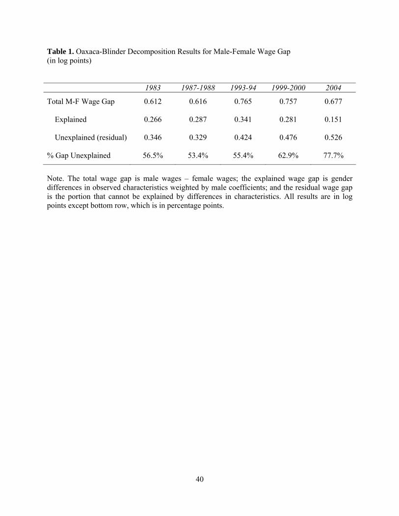
40
Table 1. Oaxaca-Blinder Decomposition Results for Male-Female Wage Gap (in log points) 1983 1987-1988 1993-94 1999-2000 2004
Total M-F Wage Gap 0.612 0.616 0.765 0.757 0.677 Explained 0.266 0.287 0.341 0.281 0.151 Unexplained (residual) 0.346 0.329 0.424 0.476 0.526 % Gap Unexplained 56.5% 53.4% 55.4% 62.9% 77.7%
Note. The total wage gap is male wages – female wages; the explained wage gap is gender differences in observed characteristics weighted by male coefficients; and the residual wage gap is the portion that cannot be explained by differences in characteristics. All results are in log points except bottom row, which is in percentage points.

41
Table 2. Index of Domestic Concentration, 1980-2004 ISIC Industry Label (1-No. Establishments/Output)
More Concentrated 353 Petroleum refinery 0.999 351 Industrial chemicals 0.978 371 Iron and steel 0.968 354 Miscellaneous petroleum and coal products 0.958 384 Transport equipment 0.955 313 Beverages 0.943 383 Machinery (electric) 0.940 352 Other chemicals 0.938 355 Rubber products 0.920 372 Non-ferrous metals 0.919 324 Footwear (except rubber or plastic) 0.913 321 Textiles 0.909 341 Paper and products 0.906 311 Food products 0.893 382 Machinery (except electrical) 0.888
Less Concentrated 362 Glass and products 0.876 323 Leather products 0.869 385 Professional and scientific equipment 0.864 322 Wearing apparel (except footwear) 0.850 356 Plastic products 0.829 390 Other manufactured products 0.826 369 Other non-metallic mineral products 0.791 342 Printing and publishing 0.764 381 Fabricated metal products 0.763 361 Pottery, china, earthenware 0.679 314 Tobacco 0.567 332 Furniture (except metal) 0.295 331 Wood products (except furniture) 0.259
Note. Results show the annual average from 1980-81 to 2004-05 for the industry specific calculation (1−No. establishments/output). ISIC codes are from Revision 2. Source: Authors’ calculations based on data sources in Appendix Table 1.

42
Table 3. Employment Distribution and Female Share of the Workforce, by Industry (1983-2004) 1983 2004 Male Female % Fem. Male Female % Fem. More Concentrated Petroleum refinery 0.1 0.3 14.0 0.8 0.3 5.9 Industrial chemicals 2.9 0.0 0.0 1.7 1.4 12.2 Iron and steel 7.9 3.3 3.3 3.4 2.6 10.9 Misc. petroleum and coal products 0.1 0.0 0.0 0.4 0.2 7.8 Transport equipment 5.8 1.5 2.0 5.7 5.0 12.5 Beverages 0.6 0.2 2.4 0.6 0.8 17.9 Machinery (electric) 5.5 3.2 4.6 2.8 4.1 19.5 Other chemicals 4.8 4.6 7.3 4.1 4.9 16.4 Rubber products 1.1 0.1 0.5 1.5 1.7 15.9 Non-ferrous metals 1.2 0.2 1.6 2.4 0.8 5.2 Footwear (except rubber or plastic) 0.6 0.7 8.7 1.0 0.9 12.6 Textiles 24.5 16.7 5.3 19.9 12.3 9.2 Paper and products 1.5 0.6 3.2 3.9 0.4 1.6 Food products 9.7 5.7 4.5 9.0 8.7 13.7 Machinery (except electrical) 6.2 0.9 1.2 6.2 3.2 7.7 Less Concentrated Glass and products 1.1 1.3 9.1 0.7 4.6 53.2 Leather products 0.6 0.8 9.8 0.8 1.1 18.7 Professional and scientific equipment 0.6 0.6 7.4 0.4 0.2 9.3 Wearing apparel (except footwear) 3.2 7.6 16.1 6.3 11.7 23.1 Plastic products 1.1 0.9 6.5 2.8 1.1 6.3 Other manufactured products 3.0 1.8 4.7 4.2 2.2 8.0 Other non-metallic mineral products 3.9 3.5 6.8 3.9 3.1 11.2 Printing and publishing 3.6 3.3 7.0 4.4 4.6 14.6 Fabricated metal products 4.8 1.3 2.2 6.7 3.7 8.4 Pottery china earthenware 0.2 0.6 21.5 0.0 0.3 56.3 Tobacco 2.4 39.7 58.0 2.0 16.2 56.7 Furniture (except metal) 0.6 0.0 0.0 2.1 1.5 10.3 Wood products (except furniture) 2.3 0.6 1.9 2.7 2.1 11.1 All Industries Total 100.0 100.0 7.6 100.0 100.0 14.0 More Concentrated Total 72.7 38.0 4.1 63.2 47.5 10.9 Less Concentrated Total 27.3 62.0 15.7 36.8 52.5 18.8 Source: Authors’ calculations using population-weighted averages based on NSSO data.

43
Table 4. Ordinary Least Squares Estimates of Male-Female Residual Wage Gaps by Industry (in log points; standard errors in parentheses). Model 1 Model 2 Model 3 Model 4 Model 5 Model 6
Concentration 0.441 0.037 0.945 -0.020 0.149 0.532 (0.435) (0.302) (0.648) (0.210) (0.131) (0.430) Trade 0.384* 0.130 0.489** 0.124 0.076 0.272 (0.205) (0.140) (0.213) (0.141) (0.078) (0.189) Year 0.380* 0.023 0.433 1.073** 0.272 1.492* (0.204) (0.201) (0.322) (0.548) (0.414) (0.904) Concen x Trade -0.390 -0.289* -0.614** -0.108 -0.207** -0.378 (0.262) (0.159) (0.267) (0.181) (0.092) (0.241) Concen x Year -0.373* 0.003 -0.446 -1.149* -0.276 -1.702 (0.225) (0.225) (0.356) (0.634) (0.498) (1.061) Trade x Year -0.179** -0.029 -0.190* -0.430* -0.137 -0.598* (0.088) (0.096) (0.111) (0.221) (0.253) (0.336) Concen x Trade x Year 0.197** 0.054 0.222* 0.496* 0.214 0.730* (0.099) (0.106) (0.123) (0.260) (0.297) (0.399) Constant -0.328 0.280 -0.587 0.166 0.234** -0.118 (0.380) (0.274) (0.533) (0.167) (0.112) (0.296) No. observations 140 140 140 140 140 140 R2 0.095 0.202 0.081 0.085 0.186 0.068
Note. The dependent variable across models is the residual wage gap. In Models 1 and 4, trade is exports/output; in Models 2 and 5, trade is imports/output; and in Models 3 and 6, trade is (exports+imports)/output. Also, in Models 1 through 3, year is a time trend; and in Models 4 through 6, year is a post-liberalization dummy. We weighted all regressions with industry-level employment shares, and standard errors are clustered by industry to adjust for intra-industry correlation. The notation *** denotes statistically significant at the 0.01 level; ** at the 0.05 level, and * at the 0.10 level.

44
Table 5. Fixed Effects Estimates of Male-Female Residual Wage Gaps by Industry (in log points; standard errors in parentheses). Model 1 Model 2 Model 3 Model 4 Model 5 Model 6
Concentration 0.538 -0.633 0.701 0.531 -0.287 0.454 (0.532) (0.465) (0.565) (0.551) (0.417) (0.590) Trade 0.630*** 0.192 0.606*** 0.468** 0.088 0.442** (0.208) (0.177) (0.214) (0.216) (0.139) (0.212) Year 0.340 0.040 0.388 0.593 0.223 1.049 (0.270) (0.172) (0.327) (0.577) (0.325) (0.801) Concen x Trade -0.747*** -0.248 -0.635** -0.510** -0.101 -0.398 (0.246) (0.197) (0.248) (0.249) (0.153) (0.246) Concen x Year -0.328 0.013 -0.417 -0.728 -0.168 -1.318 (0.281) (0.187) (0.335) (0.669) (0.383) (0.943) Trade x Year -0.190* -0.026 -0.174 -0.402 -0.093 -0.463 (0.109) (0.069) (0.117) (0.251) (0.195) (0.313) Concen x Trade x Year 0.224* 0.038 0.207* 0.526* 0.124 0.590 (0.116) (0.071) (0.121) (0.296) (0.221) (0.367) No. observations 140 140 140 140 140 140 R2 0.718 0.705 0.715 0.706 0.691 0.705
Note. The dependent variable across models is the residual wage gap. In Models 1 and 4, trade is exports/output; in Models 2 and 5, trade is imports/output; and in Models 3 and 6, trade is (exports+imports)/output. Also, in Models 1 through 3, year is a time trend; and in Models 4 through 6, year is a post-liberalization dummy. All regressions are weighted with industry-level employment shares. The notation *** denotes statistically significant at the 0.01 level; ** at the 0.05 level, and * at the 0.10 level.

45
Figure 1. Trade Ratios and Male-Female Residual Wage Gap, 1980-2004 Source: Authors’ calculations based on data sources in Appendix Table 1.
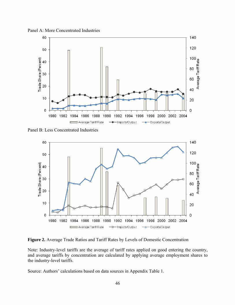
46
Panel A: More Concentrated Industries
Panel B: Less Concentrated Industries
Figure 2. Average Trade Ratios and Tariff Rates by Levels of Domestic Concentration Note: Industry-level tariffs are the average of tariff rates applied on good entering the country, and average tariffs by concentration are calculated by applying average employment shares to the industry-level tariffs. Source: Authors’ calculations based on data sources in Appendix Table 1.

47
Figure 3. Skill Intensity and Capital Intensity by Levels of Domestic Concentration, 1980-2004 Note: Skill intensity is constructed as the number of workers with college or above, relative to the number of workers with less education. Capital intensity is constructed as fixed capital relative to output. Source: Authors’ calculations based on data sources in Appendix Table 1.

48
Appendix Table 1. Descriptive and Regression Analyses: Variables and Data Sources Variable Description Data Source and Years Covered
Male wages − female wages, by industry National Sample Survey Organization (NSSO): Gender Wage Gap (unadjusted wages and residual wages) 1983, 1987-88, 1993-94, 1999-2000, 2004.
Wage Deflator Wholesale price index for manufactured products Ministry of Commerce and Industry, Government of India: 1980-81 – 2004-05.
Export Value Dollar value of India’s exports, by industry Trade, Production and Protection Database (Nicita & Olarreaga 2006): 1980 – 2004.
Import Value Dollar value of India’s imports, by industry Trade, Production and Protection Database (Nicita & Olarreaga 2006): 1980 – 2004.
Tariffs Average tariff rates, by industry Trade, Production and Protection Database (Nicita & Olarreaga 2006): 1990, 92, 97, 99, 2001, 04
Gang and Pandey (1998a,b): 1983, 1989. Domestic Output Total output, in rupees, by industry
Annual Survey of Industries (ASI): 1980-81 – 2004-05.
Exchange Rate Average annual rupee/US$ exchange rate Reserve Bank of India: 1980-81 – 2004-05.
Domestic Concentration (1 – No. establishments/output), by industry Annual Survey of Industries (ASI): 1980-81 – 2004-05.

49
Appendix Table 2. Concordance Between ISIC Revision 2, NIC 1970, NIC 1987, NIC 1998, and NIC 2004 Codes Labels ISIC NIC 1970 NIC 1987 NIC 1998 NIC 2004
Food products 311-2 200-219 200-219 1511-1549 1511-1549 Beverages 313 220-224 220-224 1551-1554 1551-1554 Tobacco 314 225-229 225-229 1600 1600 Textiles 321 230-263, 266-269 230-264, 267-269 1711-1730 1711-1730 Wearing apparel (except footwear) 322 264-265 265-266 1810 1810 Leather products 323 290, 292-293, 295-299 290, 292-293, 295-299 1820-1912 1820-1912 Footwear (except rubber or plastic) 324 291 291 1920 1920 Wood products (except furniture) 331 270-275, 279 270-275, 279 2010-2029 2010-2029 Furniture (except metal) 332 276-277 276-277 3610 3610 Paper and products 341 280-283 280-283 2101-2109 2101-2109 Printing and publishing 342 284-289 284-289 2211-2230 2211-2230 Industrial chemicals 351 294, 310-311, 316 294, 300-302, 306 2411-2413, 2430 2411-2413, 2430 Other chemicals 352 312-315, 317-319 303-305, 307-309 2421-2429 2421-2429 Petroleum refinery 353 304 314-315 2320 2320 Miscellaneous petroleum and coal products 354 305-307 316-319 2310, 2330 2310, 2330 Rubber products 355 300-302 310-312 2511-2519 2511-2519 Plastic products 356 303 313 2520 2520 Pottery, china, earthenware 361 322-323 322-323 2691 2691 Glass and products 362 321 321 2610 2610 Other non-metallic mineral products 369 320, 324-329 320, 324-329 2692-2699 2692-2699 Iron and steel 371 330-332 330-332 2710 2711-2719 Non-ferrous metals 372 333-339, 344 333-339, 344-345 2720-2732, 2891-2892 2720-2732, 2891-2892 Fabricated metal products 381 340-343, 345-349 340-343, 346-349 2811-2812, 2893-2899 2811-2812, 2893-2899 Machinery (except electrical)
382
350-359
350-359, 388, 390-394, 397-399
2813, 2911-2930, 3000
2813, 2911-2930, 3000
Machinery (electric) 383 360-369 360-369, 395-396 3110-3230 3110-3230 Transport equipment 384 370-379 370-379 3410-3599 3410-3599 Professional and scientific equipment 385 380-382 380-382 3311-3330 3311-3330 Other manufactured products 390 383-389 383-387, 389 3691-3699 3691-3699 Source: Created by authors, with reference to Sivadasan and Slemrod (2006) and Central Statistical Organization (1970, 1987, 1998, 2004).

50
Appendix Table 3. Summary Statistics for Regular Salaried Wage Earners in Manufacturing, 1983-2004 Male 1983 Female 1983 Male 2004 Female 2004 Variable Log real weekly cash wages in rupees 4.055 3.443 4.816 4.138 (1.015) (0.900) (0.936) (1.113) Dummy for illiterate individual 0.151 0.455 0.095 0.303 (0.359) (0.498) (0.294) (0.460) Dummy for individual with below primary years of schooling 0.135 0.137 0.056 0.035 (0.342) (0.344) (0.230) (0.184) Dummy for individual with primary school 0.197 0.114 0.160 0.158 (0.398) (0.318) (0.367) (0.365) Dummy for individual with middle school 0.199 0.108 0.272 0.119 (0.399) (0.310) (0.445) (0.325) Dummy for individual with secondary school 0.231 0.150 0.251 0.157 (0.421) (0.357) (0.433) (0.364) Dummy for individual with graduate school 0.087 0.037 0.166 0.228 (0.281) (0.190) (0.372) (0.420) Years of potential experience for individual 20.542 19.605 18.092 19.509 (11.920) (12.361) (11.060) (12.712) Years of potential experience for individual squared/100 5.641 5.369 4.496 5.419 (5.894) (6.070) (5.000) (5.929) Dummy for individual with no technical education 0.913 0.945 0.874 0.896 (0.281) (0.228) (0.332) (0.306) Dummy for individual who is currently married 0.752 0.596 0.698 0.643 (0.432) (0.491) (0.459) (0.480) Dummy for scheduled-tribe/scheduled-caste individual 0.154 0.200 0.166 0.156 (0.361) (0.400) (0.372) (0.364) Dummy for self-employed individual 0.084 0.168 0.060 0.130 (0.277) (0.374) (0.238) (0.336) Dummy for individual of Hindu religion 0.843 0.827 0.856 0.878 (0.364) (0.379) (0.351) (0.328) Dummy for households with male heads 0.967 0.770 0.951 0.767 (0.178) (0.421) (0.216) (0.423) Dummy for rural areas 0.222 0.395 0.286 0.413 (0.415) (0.489) (0.452) (0.493) Number of pre-school children in household 0.599 0.557 0.450 0.280 (0.844) (0.847) (0.728) (0.616) Dummy for northern states of India 0.206 0.122 0.261 0.078 (0.404) (0.328) (0.439) (0.269) Dummy for southern states of India 0.254 0.507 0.248 0.479 (0.435) (0.500) (0.432) (0.500) Dummy for eastern states of India 0.174 0.059 0.070 0.071 (0.379) (0.235) (0.254) (0.258) Dummy for western states of India 0.367 0.312 0.420 0.371 (0.482) (0.464) (0.494) (0.484) Number of observations 10909 834 3540 548
Standard deviations in parentheses. Sample in each year consists of regular salaried workers between 15-60 years of age with positive cash wages in the manufacturing industry. Our regressions include interactions of the potential experience variables and the education dummies.
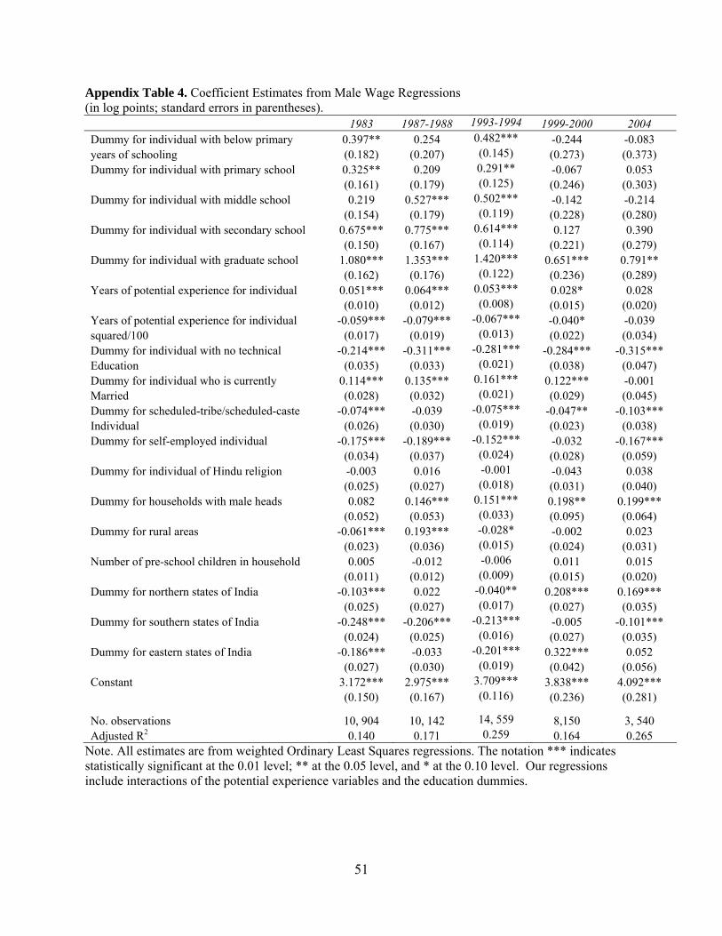
51
Appendix Table 4. Coefficient Estimates from Male Wage Regressions (in log points; standard errors in parentheses). 1983 1987-1988 1993-1994 1999-2000 2004 Dummy for individual with below primary 0.397** 0.254 0.482*** -0.244 -0.083 years of schooling (0.182) (0.207) (0.145) (0.273) (0.373) Dummy for individual with primary school 0.325** 0.209 0.291** -0.067 0.053 (0.161) (0.179) (0.125) (0.246) (0.303) Dummy for individual with middle school 0.219 0.527*** 0.502*** -0.142 -0.214 (0.154) (0.179) (0.119) (0.228) (0.280) Dummy for individual with secondary school 0.675*** 0.775*** 0.614*** 0.127 0.390 (0.150) (0.167) (0.114) (0.221) (0.279) Dummy for individual with graduate school 1.080*** 1.353*** 1.420*** 0.651*** 0.791** (0.162) (0.176) (0.122) (0.236) (0.289) Years of potential experience for individual 0.051*** 0.064*** 0.053*** 0.028* 0.028 (0.010) (0.012) (0.008) (0.015) (0.020) Years of potential experience for individual -0.059*** -0.079*** -0.067*** -0.040* -0.039 squared/100 (0.017) (0.019) (0.013) (0.022) (0.034) Dummy for individual with no technical -0.214*** -0.311*** -0.281*** -0.284*** -0.315*** Education (0.035) (0.033) (0.021) (0.038) (0.047) Dummy for individual who is currently 0.114*** 0.135*** 0.161*** 0.122*** -0.001 Married (0.028) (0.032) (0.021) (0.029) (0.045) Dummy for scheduled-tribe/scheduled-caste -0.074*** -0.039 -0.075*** -0.047** -0.103*** Individual (0.026) (0.030) (0.019) (0.023) (0.038) Dummy for self-employed individual -0.175*** -0.189*** -0.152*** -0.032 -0.167*** (0.034) (0.037) (0.024) (0.028) (0.059) Dummy for individual of Hindu religion -0.003 0.016 -0.001 -0.043 0.038 (0.025) (0.027) (0.018) (0.031) (0.040) Dummy for households with male heads 0.082 0.146*** 0.151*** 0.198** 0.199*** (0.052) (0.053) (0.033) (0.095) (0.064) Dummy for rural areas -0.061*** 0.193*** -0.028* -0.002 0.023 (0.023) (0.036) (0.015) (0.024) (0.031) Number of pre-school children in household 0.005 -0.012 -0.006 0.011 0.015 (0.011) (0.012) (0.009) (0.015) (0.020) Dummy for northern states of India -0.103*** 0.022 -0.040** 0.208*** 0.169*** (0.025) (0.027) (0.017) (0.027) (0.035) Dummy for southern states of India -0.248*** -0.206*** -0.213*** -0.005 -0.101*** (0.024) (0.025) (0.016) (0.027) (0.035) Dummy for eastern states of India -0.186*** -0.033 -0.201*** 0.322*** 0.052 (0.027) (0.030) (0.019) (0.042) (0.056) Constant 3.172*** 2.975*** 3.709*** 3.838*** 4.092*** (0.150) (0.167) (0.116) (0.236) (0.281)
No. observations 10, 904 10, 142 14, 559 8,150 3, 540 Adjusted R2 0.140 0.171 0.259 0.164 0.265
Note. All estimates are from weighted Ordinary Least Squares regressions. The notation *** indicates statistically significant at the 0.01 level; ** at the 0.05 level, and * at the 0.10 level. Our regressions include interactions of the potential experience variables and the education dummies.
Recommended