Forschungsinstitut zur Zukunft der ArbeitInstitute for the Study of Labor
DI
SC
US
SI
ON
P
AP
ER
S
ER
IE
S
Integrated Macroeconomic Production Functionfor Open Economies:A New Schumpeterian Solow Model for Globalization
IZA DP No. 9724
February 2016
Paul J.J. Welfens

Integrated Macroeconomic Production
Function for Open Economies: A New Schumpeterian Solow Model for
Globalization
Paul J.J. Welfens EIIW and Schumpeter School, University of Wuppertal, Sciences Po, IZA and AICGS/Johns Hopkins University
Discussion Paper No. 9724 February 2016
IZA
P.O. Box 7240 53072 Bonn
Germany
Phone: +49-228-3894-0 Fax: +49-228-3894-180
E-mail: [email protected]
Any opinions expressed here are those of the author(s) and not those of IZA. Research published in this series may include views on policy, but the institute itself takes no institutional policy positions. The IZA research network is committed to the IZA Guiding Principles of Research Integrity. The Institute for the Study of Labor (IZA) in Bonn is a local and virtual international research center and a place of communication between science, politics and business. IZA is an independent nonprofit organization supported by Deutsche Post Foundation. The center is associated with the University of Bonn and offers a stimulating research environment through its international network, workshops and conferences, data service, project support, research visits and doctoral program. IZA engages in (i) original and internationally competitive research in all fields of labor economics, (ii) development of policy concepts, and (iii) dissemination of research results and concepts to the interested public. IZA Discussion Papers often represent preliminary work and are circulated to encourage discussion. Citation of such a paper should account for its provisional character. A revised version may be available directly from the author.

IZA Discussion Paper No. 9724 February 2016
ABSTRACT
Integrated Macroeconomic Production Function for Open Economies:
A New Schumpeterian Solow Model for Globalization* The macroeconomic production function is a traditional key element of modern macroeconomics, as is the more recent knowledge production function which explains knowledge/patents by certain input factors such as research, foreign direct investment or international technology spillovers. This study is a major contribution to innovation, trade, FDI and growth analysis, namely in the form of a combination of an empirically relevant knowledge production function for open economies – with both trade and inward FDI as well as outward foreign direct investment plus research input – with a macro production function. Plugging the open economy knowledge production function into a standard macroeconomic production function yields important new insights for many fields: The estimation of the production potential in an open economy, growth decomposition analysis in the context of economic globalization and the demand for labor as well as long run international output interdependency of big countries; and this includes a view at the asymmetric case of a simple two country world in which one country is at full employment while the other is facing underutilized capacities. Finally, there are crucial implications for the analysis of broad regional integration schemes such as TTIP or TPP and a more realistic and comprehensive empirical analysis. JEL Classification: E23, F02, F62, 011, 032 Keywords: potential output, innovation, knowledge production function, macroeconomics,
globalization Corresponding author: Paul J.J. Welfens European Institute for International Economic Relations University of Wuppertal Rainer-Gruenter-Straße 21 D-42119 Wuppertal Germany E-mail: [email protected]
* I gratefully acknowledge discussions with and research assistance by Jens Perret and Vladimir Udalov as well as editorial assistance by David Hanrahan. Particular thanks go to Andre Jungmittag, Frankfurt School of Applied Sciences, for stimulating discussion – the reader is also referred to the companion empirical paper EIIW No. 212. The usual disclaimer applies. This paper is dedicated to the late Edward Graham, Petersen Institute for International Economics – he has conducted crucial research on foreign direct investment in the world economy.

IV
Integrated Macroeconomic Production Function for Open
Economies: A New Schumpeterian Solow Model for Globalization
Table of Contents
Table of Contents .............................................................................................................. IV
List of Tables ........................................................................................................................V
1. Introduction ................................................................................................................. 1
2. Knowledge Production Function and Macroeconomic Production Function ....... 4 2.1 Theoretical Aspects of the Knowledge Production Function ................................ 4
3. The Schumpeterian Macroeconomic Production Function .................................... 8 3.1 Output Elasticity with Respect to Foreign Knowledge ....................................... 11 3.2 Endogenous Growth Model ................................................................................ 11
3.3 Golden Rule ......................................................................................................... 12 3.4 Labor Market Demand and other Macro Aspects ............................................... 13
3.5 Hybrid Medium-Term Macro Model .................................................................. 14 3.6 Further Extensions ............................................................................................... 15
4. Policy Conclusions ..................................................................................................... 15
References .......................................................................................................................... 18
Appendix ............................................................................................................................ 20 Optimal Choice of the Size of the R&D Sector .............................................................. 20
Schumpeterian CES Function ......................................................................................... 20

List of Tables
Table 1: Tab. 1: Knowledge Production Function: patent applications at the
European Patent Office explained by researchers (full time equivalent), per capita
GDP (PPP, constant dollars), inward FDI-GDP ratio: panel data analysis for 20 EU
countries, 2002-2012; all variables in logs ......................................................................... 2


1
1. Introduction
The macroeconomic production function is a key element of modern macroeconomics, as
is the more recent knowledge production function which explains knowledge/patents by
certain input factors such as research or international technology spillovers. This
contribution gives an innovative consistent combination of the knowledge production
function for open economies with both trade and inward as well as outward foreign direct
investment. Macroeconomic production functions such as the Cobb-Douglas function
Y=Kß(AL)
1-ß (where output is Y, K is capital, L is labor and A is knowledge) and the CES
production function Y = (1-)(AL)-v“
+ K-v“
-1/v“ are useful workhorses of modern
Economics. For the economic analysis of a full employment economy and neoclassical
economic growth models these functions are a natural element (WELFENS, 2011).
While technological progress in a neoclassical growth model falls like manna from heaven,
a better approach is endogenous growth modeling – namely with knowledge explained in
turn by a knowledge production function which is a familiar concept in Innovation
Economics (GRILICHES, 1979; AGHION/HOWITT, 1998). The knowledge production
function is a broad concept that includes key questions such as understanding the link
between innovation dynamics - patent stocks and flows as well as entrepreneurial variables
– and total factor productivity growth as well as the spatial aspects of R&D activities and
regional innovation plus inter-regional innovation spillovers (e.g. PERRET, 2013). The
focus of analysis is at first sight rather traditional, namely to look at a macroeconomic
knowledge production function which has received some attention in the earlier literature
(e.g. MACHLUP, 1979) and which also has complementary research strands with a focus
on sectoral knowledge production functions (e.g. for Germany: BÖNTE, 2001). Open
economy aspects thus far were mainly considered in the context of intermediate
technology-intensive input imports and related questions relevant for total factor
productivity growth (e.g. COE/HELPMAN, 1995); with respect to the empirical relevance
of this concept KELLER (2000) has raised crucial objections. JUNGMITTAG (2004) has
emphasized the role of trade and high-technology specialization for economic catching-up
in an empirical EU context. The globalization of innovation – and hence the role of
multinational companies - has received increasing attention since the beginning of the 21st
century (e.g. NARULA/ZANFEI, 2005; UNCTAD, 2005, VEUGELERS, 2005), however,
it has not been much considered in international macroeconomics and regional integration
analysis although deep integration projects, such as the EU-US project TTIP (Transatlantic
Trade and Investment Partnership) or the project TPP (Trans-Pacific Partnership) of the US
with countries around the Pacific Basin, suggest to consider the interaction of trade, FDI,
innovation and output dynamics simultaneously – and not to focus solely on trade
dynamics. Given recent studies which look in a micro perspective at the link between FDI
and trade or innovation and exports (e.g. DUNNING/LUNDAN, 2008;
LACHENMAIER/WÖSSMANN, 2006), one may argue that there is broad empirical
evidence for some links at the micro level or the sectoral level, but standard international
macroeconomics has not integrated FDI, innovation and trade in a systematic way.
The special feature considered here is the simultaneous open economy focus on trade and
FDI for knowledge production – and the link of knowledge dynamics with macroeconomic
output dynamics. The following approach is a major analytical innovation for the case of

an open economy with imports and exports of goods and services and both inward foreign
direct investment and outward FDI. Applying this concept to 20 EU countries has resulted
in clear empirical evidence supporting this approach (JUNGMITTAG/WELFENS, 2016)
as the regression analysis shows.
Table 1: Tab. 1: Knowledge Production Function: patent applications at the
European Patent Office explained by researchers (full time equivalent), per capita
GDP (PPP, constant dollars), inward FDI-GDP ratio: panel data analysis for 20
EU countries, 2002-2012; all variables in logs
Dependent Variable: LOG(PAT?) Method: Pooled Least Squares Date: 01/14/16 Time: 17:10 Sample: 2002 2012 Included observations: 11 Cross-sections included: 20 Total pool (unbalanced) observations: 205
Variable Coefficient Std. Error t-Statistic Prob. C -16.75261 1.936751 -8.649851 0.0000
LOG(RDPERS?) 0.354843 0.091091 3.895492 0.0001 LOG(PGDPDOLLAR?) 1.819009 0.194151 9.369062 0.0000 LOG(FDISTOCKQ?) 0.164400 0.074407 2.209453 0.0284 Fixed Effects (Cross)
_AT--C 0.522542 _BE--C 0.384865 _CZ--C -0.911734 _DK--C 0.118808 _FI—C 0.432950 _FR--C 1.701492 _DE--C 2.471143 _GR--C -1.365439 _HU--C -0.343212 _IE—C -1.054935 _IT—C 1.424113 _LU--C -2.833316 _NL--C 0.804435 _PL--C -0.270742 _PT--C -1.450550 _SK--C -1.585013 _SI—C -0.856756 _ES--C 0.238784 _SE--C 0.739902 _UK--C 1.326632
Effects Specification Cross-section fixed (dummy variables) R-squared 0.993230 Mean dependent var 6.740298
Adjusted R-squared 0.992411 S.D. dependent var 1.795015 S.E. of regression 0.156371 Akaike info criterion -0.767790 Sum squared resid 4.450218 Schwarz criterion -0.394964 Log likelihood 101.6984 Hannan-Quinn criter. -0.616991 F-statistic 1213.621 Durbin-Watson stat 1.052678 Prob(F-statistic) 0.000000
Source: JUNGMITTAG/WELFENS (2016), Tab. 1, forthcoming
The approach presented here suggests a consistent integration of the knowledge production
function in the macroeconomic production function and it seems obvious that this two-

3
pronged analytical perspective on knowledge and output is useful for a world economy
characterized by globalzation and innovation. In the US, Europe and China/ASEAN, trade
and foreign direct investment have played an increasing role both in the form of inward
FDI and as outward FDI (KRUGMAN/GRAHAM, 1995; UNCTAD, 2014; ADB, 2015;
WORLD BANK, 2016).
The knowledge production function suggested here is straightforward and its implication
for a Cobb-Douglas production function likewise – it is very interesting and allows a much
better understanding of some key economic questions than previously. Plugging the
knowledge production function – that is empirically robust – into a standard
macroeconomic production function yields important new insights for many fields: The
estimation of the production potential in an open economy, growth decomposition analysis
in the context of economic globalization and the demand for labor, as well as long run
international output interdependency of big countries – and this includes a view at the
asymmetric case of a simple two country world in which one country is at full employment
while the other is facing underutilized capacities. Estimation of the production potential is
important in many ways, not least for the analysis of structural budget deficits and capacity
utilization. Finally, the debate about output multipliers can be stated within the new
framework in a different way than was the case in the traditional debate. Since economic
globalization has continued for decades – with trade intensities and cumulated FDI inflows
and FDI outflows (relative to GDP) increasing – it is important to get a better
understanding of the supply-side dynamics in open economies.
There is clear evidence that over time the export-GDP ratio and the import-GDP ratio in
OECD countries as well as in NICs are growing. A similar observation holds for the ratio
of inward FDI stocks in OECD countries, since about 1985, and also for outward FDI
stocks of OECD countries (and for some newly industrialized countries this also holds).
The following section states at first a knowledge production function which can be
considered as robust with respect to OECD countries; here the intensity of exports (x:=
X/Y where X is export volume) and the intensity of imports (j:= J/Y; where J stands for the
real import volume) as well as the share of cumulated inward FDI in the total capital stock
(*) and the share () outward cumulated FDI in the foreign capital stock as well as the
share of researchers in the total labor force is crucial; plus some other variables. The next
step is to plug the knowledge production function into the production function and to take
a closer look at some key implications, including the marginal product of labor and long
run labor demand, respectively. There also are several key implications for the supply side
and growth dynamics in open economies – and also selected policy implications will have
to be considered.
The Schumpeterian Macro Production Function obtained from plugging the knowledge
production function for an open economy brings many new insights; these include:
a new understanding of the rather complex input factors that determine output in an
open economy with inward and outward FDI, trade and research activities; this
includes the complex elasticity of output with respect to foreign knowledge
a new view on the long term interdependency of output in a two country approach
an empirically valid endogenous growth model (with analytical solutions restricted
to certain parameter conditions)

a new solution for the golden rule
a new view on the role of domestic and foreign real money balances for domestic
full employment equilibrium output
a clear understanding that in an economy with trade and two-way FDI the long run
foreign output growth rate will be one of the determinants of long run steady state
economic growth – along with specific parameters from the knowledge production
function
a better – more realistic – basis for supply-side policy actions in open economies.
One also can easily understand that this includes opportunities for international
policy cooperation.
2. Knowledge Production Function and Macroeconomic
Production Function
Since the Industrial Revolution, the creation of new knowledge has been a key driver of
economic growth. Patent protection has been the institutional innovation that has
stimulated innovation in the industrial sector since the 1830s (with the temporary notable
exceptions of Switzerland and Netherlands which had no patent protection for some time
as an ultra-liberal position taken by society and government suggested that having no
intellectual property rights would be the best way to stimulate new knowledge). The
modern economy in which services are dominating in terms of value-added and
employment still has a crucial industrial core and patent applications continue to be a
valuable indicator for innovation dynamics – although part of innovation dynamics is
covered by copyrights and, in certain fields, through the very speed of innovation waves -
as is the case, for example, in part of the digital economy. As regards international trade in
new knowledge, there is broad consensus amongst economists that technological
information/knowledge markets are very imperfect since revealing part of knowledge for
free is required in order for potential buyers to assess the economic value of the respective
innovation. At the same time, there is the problem of asymmetric information and
opportunistic behavior which implies rather low opportunities for patent trading; most
international exchange of new knowledge is in the form of intra-company licenses in
multinational companies or cross-licensing among MNCs.
2.1 Theoretical Aspects of the Knowledge Production Function
In an open economy it is straightforward to assume that trade intensity – proxied through
X/Y or X/L and J/Y or J/L, respectively – will contribute to knowledge A (X is export
volume, J is import volume; is the share of country 1 investors’ ownership of the foreign
capital stock K*; * is the share of foreign ownership of the capital stock K of country 1,);
on the import side, intermediate technology-intensive products in particular should
contribute to raising knowledge in line with the arguments of COE/HELPMAN (1995)
and a high export intensity should also put pressure on the aggregate of firms to raise
knowledge, namely in line with MELITZ (2003) whose argument is that in a world with

5
heterogeneous firms, opening up for trade will allow the most productive firms to expand
through exports while the weakest firms, in terms of productivity and knowledge,
respectively, will leave the market. Moreover, the size of the R&D sector (z“ is the share
of output devoted to R&D) and the share of cumulated inward FDI relative to K (*) - or
to Y - plus the sourcing of foreign technologies abroad through relative outward FDI
stocks (proxied by K*/Y* or K*/K) should contribute to knowledge. Inward FDI stock
is naturally associated with intra-company international technology transfer from the
headquarter to subsidiaries, a high outward FDI stock in technologically leading OECD
countries should allow to tap foreign technological progress through asset-seeking FDI –
and in this context not least through regional innovation spillovers abroad as well as
through R&D projects conducted abroad. Hence, with positive parameters H, V’, V“, V
and V*, one can state the knowledge production function as follows:
(1”) A = (X/L)H (J/L)
V’ (z“Y)
V“(*K/Y)
V (K*/Y*)
V*
As regards the international technology transfer from abroad one might consider
alternatively to (K*/Y*) the variable K*/Y since the asset-seeking (knowledge-seeking)
cumulated outward FDI relative to the GDP of the source country of FDI could be the
relevant indicator – empirical analysis has to clarify this point (note that K*/Y can be
rewritten as (K*/Y*)(Y*/Y) so that the subsequently derived integrated Schumpeterian
macroeconomic production function – with the knowledge production function integrated
into the macro production function – would have to be slightly reformulated). The equation
stated to some extent seems to be in line with the skeptical view of JONES (1995) who has
raised some doubts about the rather optimistic view of ROMER (1990) who suggests that
the number of researchers determines the growth rate of knowledge; JONES uses total
factor productivity (TFP) as a measure of knowledge. Interestingly, the model presented
here suggests that the foreign rate of technological progress as well as the domestic level of
knowledge contribute to output expansion: A determines the level of the output growth
path, but the model with an exogenous foreign growth rate of knowledge (a*) implies that
the trend growth rate of GDP in country 1 is affected by a*. ABDIH/JOUTZ (2005) -
using patents to proxy the stock of knowledge - have argued with respect to the USA that a
simple knowledge production function could be stated as dA/dt = a’L’a”
Ac”
(t is time, L’ is
the number of researchers, a’, a” and c” are positive parameters) and the authors estimate a
long run relationship: that doubling the stock of knowledge (patent stock) will raise TFP by
only 10 percent in the long run.
The approach developed here follows the above equation (1”) and some standard equations
from macroeconomics:
Assuming X= xY* and J=jY one may write (0<x<1; 0<j<1):
(2”) A = (xyY*/Y)H (jy)
V’(z“Y)
V“(*K/Y)
V (K*/Y*)
V*
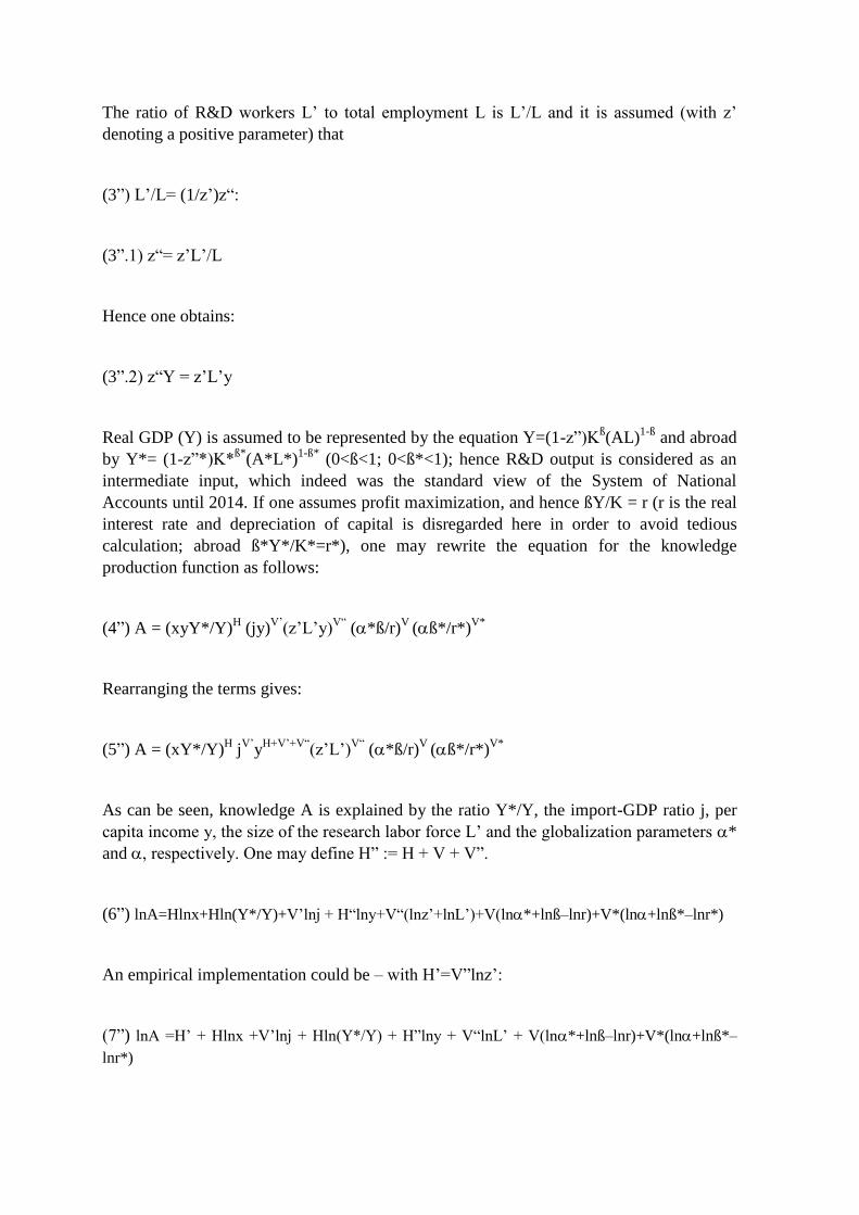
The ratio of R&D workers L’ to total employment L is L’/L and it is assumed (with z’
denoting a positive parameter) that
(3”) L’/L= (1/z’)z“:
(3”.1) z“= z’L’/L
Hence one obtains:
(3”.2) z“Y = z’L’y
Real GDP (Y) is assumed to be represented by the equation Y=(1-z”)Kß(AL)
1-ß and abroad
by Y*= (1-z”*)K*ß*
(A*L*)1-ß*
(0<ß<1; 0<ß*<1); hence R&D output is considered as an
intermediate input, which indeed was the standard view of the System of National
Accounts until 2014. If one assumes profit maximization, and hence ßY/K = r (r is the real
interest rate and depreciation of capital is disregarded here in order to avoid tedious
calculation; abroad ß*Y*/K*=r*), one may rewrite the equation for the knowledge
production function as follows:
(4”) A = (xyY*/Y)H (jy)
V’(z’L’y)
V“ (*ß/r)
V (ß*/r*)
V*
Rearranging the terms gives:
(5”) A = (xY*/Y)H j
V’y
H+V’+V“(z’L’)
V“ (*ß/r)
V (ß*/r*)
V*
As can be seen, knowledge A is explained by the ratio Y*/Y, the import-GDP ratio j, per
capita income y, the size of the research labor force L’ and the globalization parameters *
and , respectively. One may define H” := H + V + V”.
(6”) lnA=Hlnx+Hln(Y*/Y)+V’lnj + H“lny+V“(lnz’+lnL’)+V(ln*+lnß–lnr)+V*(ln+lnß*–lnr*)
An empirical implementation could be – with H’=V”lnz’:
(7”) lnA =H’ + Hlnx +V’lnj + Hln(Y*/Y) + H”lny + V“lnL’ + V(ln*+lnß–lnr)+V*(ln+lnß*–
lnr*)

7
This is a compact theoretical basis for the empirical analysis of a knowledge production
function with inward cumulated FDI and outward cumulated FDI; if one assumes, roughly
in line with a Heckscher-Ohlin setting, that production technology at home is the same as
abroad with respect to ß and ß* (ß=ß*), respectively, and if capital mobility brings about
r=r*, a setup with V=V“ allows to consider the simplified equation for empirical
implementation (otherwise the more complex version would have to be used):
(8”) lnA = H’ + Hlnx + V’lnj + Hln(Y*/Y) + H“lny + V“lnL’ + Vln*+ Vln
Trade globalization would show up in the form of a rise of x and j, and FDI globalization
in the form of a rise of * and , respectively. While this formulation of the knowledge
production formation is fairly straightforward, it is a priori not clear how well the
empirical implementation will work. It is noteworthy that one may define a global
economic equilibrium through the condition that Y*/Y as well as the parameters x, j, , *
should be constant. If Y/(AL):=y’ would be constant in a steady state situation, the
implication then is – taking into account that lny’= ln y – lnA – that the equation obviously
implies (1-H)dlnA/dt = V”dlnL’/dt. Assuming that 0<H<1, the implication then is that the
long run steady state growth rate of knowledge is given by:
(9”) dlnA/dt = V”/(1-H)dlnL’/dt
This equation can be understood easily if one assumes that the growth rate of researchers
dlnL’/dt is constant, however, this implies skilled labor dynamics and human capital
formation – assuming that research is skill-intensive. With respect to empirical analysis
and panel data analysis, one may emphasize that OECD countries differ in the degree of
two-way FDI intensity; many countries have relatively high FDI inflows, but rather small
relative FDI outflows, but fixed country effects in panel data analysis should cover this and
other aspects. For small open economies the analysis is rather straightforward, more
complicated is the situation of international technology or macroeconomic
interdependency. International technology interdependency could be related to techno-
globalization (JUNGMITTAG, 2016; DACHS, 2016; DACHS ET AL., 2015) or to the
oligopolistic international interdependency of multinational companies’ production and
R&D activities.
An important next analytical step is to then plug the basic knowledge production function
(1”) A = (X/L)H(J/L)
V’(z“Y)
V“(*K/Y)
V(K*/Y*)
V* into the macroeconomic production
function. Hence, export per capita X/L, import per capita J/L, the output of the R&D
sector, the inward FDI stock relative to GDP and the ratio of cumulated outward FDI to
foreign GDP explain knowledge. However, in a competitive environment with a Cobb
Douglas function in both countries it has to be remembered that (1”) can be rearranged as
(5”), namely in the following compact form A = (xY*/Y)H j
V’y
H+V’+V“(z’L’)
V“ (*ß/r)
V
(ß*/r*)V*
. This formulation, which shows the impact of Y*/Y, of per capita income, of
researchers and of the inward FDI capital variable as well as the outward FDI capital
variable – plus x and j as indicators of trade intensity, is the key point of departure for the

next section. With respect to a more general knowledge production function – and its
empirical implementation – an alternative formulation of the knowledge production
function could be the equation A = (1+X/L)H (1+ J/L)
V’ (z“Y)
V“(1+*K/Y)
V
(1+K*/Y*)V*
so that the case of a closed economy with no trade and no foreign direct
investment could also be covered.
3. The Schumpeterian Macroeconomic Production Function
The Schumpeterian Macro Production Function (SMPF) is obtained from plugging the
knowledge production function into the macroeconomic production function. For the sake
of simplicity a Cobb Douglas production function Y= (1- z“)Kß(AL)
1-ß will be considered
and it is assumed here that the share z“ of R&D output in GDP is an intermediate product.
The knowledge production function is A(Y*/Y, y, L’, , *, j, x) where all partial
derivatives are positive. Using the rather compact specification of the knowledge
production function developed here, one can easily plug it into the macroeconomic
production function and in the end get a macroeconomic long run supply function (with L’
denoting the number of researchers):
Y= Y(K, L, L’, Y*, , *, x, j)
The partial derivatives are all positive. Hence let us consider the explicit result of plugging
the knowledge production function for the open economy into the macroeconomic
production function wich gives the integrated Schumpeterian production function (with
nested knowledge production function A(…)):
(I)
(II) A = (xY*/Y)H j
V’y
H+V’+V“(z’L’)
V“ (*ß/r)
V (ß*/r*)
V*
(III)
1
1 ''Y z K AL
1H H V’ V“
V“V’ V V*
1H V’ V“
V“* V’ H V’ V“ V V*
H V’ V“V“V’ V“ 1 * V’
Y* Y1 '' x j z’L’ ( * / r) ( * /r*)
Y
11 '' Y j Y z’L’ ( * / r) ( * /r*)
11 '' Y Y j z’L’
H H H
H H
Y z K ß ß LL
z K x Y ß ß LL
z K xL
1
V V*
1V“V’ V“ 1 * V’ 1 H V’ V“ V V*
1V“1 V’ V“ 1 * V’ 1 H V’ V“ V V*
( * / r) ( * /r*)
1 '' Y Y j z’L’ ( * / r) ( * /r*)
1 '' Y j z’L’ ( * / r) ( * /r*)
H H
H H
ß ß L
z K x L ß ß
Y z K x L ß ß

9
(IV)
(V)
It is obvious from the logarithmic equation that a positive growth rate dln(L’/L) will
contibute to economic output growth in the long run. To get a better understanding as to
what extent the level of the growth path and the trend growth rate itself will be affected
one will have to consider a modified neoclassical growth model.
The result obtained for the Schumpeterian macroeconomic production function looks fairly
compact. Real gross domestic product is a positive function of
the capital stock
the export-GDP ratio; and foreign GDP
the import-GDP ratio
total labor
the share of researchers in the total labor force
the ratio of the inward FDI capital stock relative to the total capital stock
the ratio of the outward FDI capital stock relative to the total capital stock abroad;
the real interest rate at home and abroad has a negative impact on the production
potential.
The latter is quite interesting since it allows a direct link to the real money supply: if
money market equilibrium – in an economy with a stable price level at home and abroad -
is written as M/P= hY/(h’r) in the home country and as M*/P*= h*Y*/(h’*r*) in country 2
(with positive parameters h, h’, h* and h’*), one gets r= hY/(h’M/P) and r*=
h*Y*/(h’*M*/P*), respectively, and thus obtains an analytical basis for monetary growth
models; defining h/h’:= h“ and h*/h’*= h“*, one can see that real money balances at home
and abroad are contributing to real GDP in an open economy with inward and outward FDI
11 1 V’ V“ 1V“* V’ 1 H V’ V“ V V*1 '' Y j z’L’ ( * / r) ( * /r*)H HY z K x L ß ß
11 1 V’ V“ 1V“* V’ 1 H V’ V“ V V*
11
V“1 V’ V“ 1 * V’ 1 H V’ V“ V V* 1 V’ V“ 11 V’ V“ 1
1 '' Y j z’L’ ( * / r) ( * /r*)
1 '' Y j z’L’ ( * / r) ( * /r*)
1ln ln 1 '' ln
1 V’ V“ 1 1 V’ V“ 1
1
1
H H
H H
Y z K x L ß ß
Y z K x L ß ß
Y z K
V“* V’ 1 H V’ V“ V V*
*
ln Y j z’L’ ( * / r) ( * /r*)V’ V“ 1
1ln 1 '' ln
1 V’ V“ 1
1 ln ln Y 'ln 1 H V’ V“ ln '' ln z’L’ ln( * / r) *ln( * /r*)
H Hx L ß ß
z K
H x H V j L V V ß V ß

(an alternative new approach in a closed economy has been suggested by WELFENS
(2011) who considers real monetary balances held by private households as an implicit
production factor of firms, namely on the basis of positive external effects for companies).
Real GDP thus can be written as follows:
There are two key insights here:
The real GDP thus is a positive function of both real money balances at home
(M/P) and real money balances abroad (M*/P*).
The exponent for K and the exponent for the large bracket term is smaller than
before so that taking into account money market equilibrium conditions at home
and abroad implies that the effective output elasticity with respect to capital and all
variables in the large bracket terms is smaller than before.
This effective Schumpeterian production potential could be the basis for a new monetary
growth model (one may, however, argue that a true monetary growth model should be
based on a production function in which M/P enters directly as a productive input, namely
in the form of positive external effects of households’ holding of real money balances M/P:
WELFENS, 2011).
Let us return to the formulation of the production potential with r and r*. It is obvious here
that if Y* is growing in a sustained way - hence the foreign economy is already in a steady
state – the implication is that the home economy is growing too; and here exports are the
key driver. As the long run level of output growth is a negative function of the real interest
rate, monetary policy can be considered in a quasi-monetary growth approach: If the
equilibrium condition for the money market is M/P= hY/(h’r), monetary policy – defined
as a change of (M/P)/Y - can reduce the real interest rate, the level of output and thus raise
output. Moreover, it can be shown that the effective Schumpeterian macro production
function implies that output per capita for the special case of ß=0.5 is a positive function of
1
1 ' '' 1
1 ' '' 1
1
1 '
1 ' '' 1
1 *''* ' 1 ' '' * * *1 ' '' 1
*** * * *1
''* ' 1 ' ''1 ' '' 1
* * *
1 '' ' ' / /
' '1 '' ' '
V V
V V
V
V V
V VVH H V H V VV V
VV
VH H V H V VV V
Y z K x Y j L z L r r
h M h MY z K x Y j L z L
YhP h Y P
'' 1
1
1 ' '' 1
1 ' '' 1
1 ' '' 1
*1 1 ' '' ** * * *1''1 ' '' 1 * ' 1 ' ''
1 ' '' 1* * *
1* ' 1 '
1 ' '' 1
' '1 '' ' '
1 ''
V
V V
V V
V V
VV V V V
VV V H H V H V VV V
H H V H V VV V
h M h MY z K x Y j L z L
hP h Y P
Y z K x Y j L
1
1 ' '' 1
1 ' '' 1
1 1 ' ''
*** * * *
''''
* * *
* * * *1''1 1 ' '' * ' 1 ' ''
1 1 ' ''* * *
' '' '
' '1 '' ' '
V V
V V
V V V
VV
V
V
VV V V H H V H V VV V V
h M h Mz L
hP h Y P
h M h MY z K x Y j L z L
hP h Y P
1* 1 1 ' ''*
V V V V

11
capital intensity, the ratio of R&D workers in the total labor force, exports per capita,
imports per capita, inward FDI intensity () and outward FDI intensity (*). For the
general case 0<ß<1 the function is more complicated. The special case of ß=0.5 allows to
develop a Schumpeterian Solow growth model on the assumption that Y*/Y is constant
and L’ is increasing at a constant rate.
3.1 Output Elasticity with Respect to Foreign Knowledge
If one wants to understand the role of foreign knowledge on country 1’s output one has to
consider the knowledge production function and the macroeconomic production in both
country 1 and country 2; recall the knowledge production function (1”) A = (X/L)H (J/L)
V’
(z“Y)V“
(*K/Y)V
(K*/Y*)V*
and the formulation (5”) A = (xY*/Y)H j
V’y
H+V’+V“(z’L’)
V“
(*ß/r)V
(ß*/r*)V*
. Let us define v:= 1 – (V’+V”)(1-ß). Hence
(6”) Y=(1-z”)Kß/v
(xHY*
HL
1-H-V-V’(z’L’)
V”(*ß/r)
V(ß*/r)
V*)(1-ß)/v
As Y*= (1-z”*)K*ß(A*L*)
1-ß we get:
(7”) Y=(1-z”)Kß/v
((xH(1-z”*)K*
ßH(A*L*)
(1-ß*)HL
1-H-V-V’(z’L’)
V”(*ß/r)
V(ß*/r)
V*)(1-ß)/v
From this follows for the effective elasticity of output with respect to foreign knowledge
that
(8”) dlnY/dlnA*= (1-ß*)H(1-ß)/v =(1-ß*)H(1-ß)/(1 – (V’+V”)(1-ß))=
=(1-ß*)H/((1-ß)-1
– (V’+V”))
Thus this elasticity of output with respect to foreign knowledge is a positive function of the
export per capita elasticity H in the knowledge production function and a negative function
of both ß* and ß (the output elasticity of capital in the macroeconomic production function
in country 1 and country 2, respectively) as well as a positive function of the import per
capita elasticity and the research output elasticity, respectively, in the knowledge
production function. Thus the theoretical analysis allows getting a much better
understanding of apparent international technology output effects.
3.2 Endogenous Growth Model
A growth model on the basis of a Schumpeterian macroeconomic production function can
be derived here in a compact endogenous growth approach. Assume for simplicity that
ß=1-ß so that ß= 0.5. Hence we can write
(9) y:= Y/L =(1-z”)k0.5/v
((xHY*
HL
-H-V-V’(z’L’)
V”(*ß/r)
V(ß*/r)
V*)0.5/v
Let us define Q:= ((xHY*
HL
-H-V-V’(z’L’)
V”(*ß/r)
V(ß*/r)
V*)
Goods market equilibrium condition in an economy with zero depreciation and constant
growth of labor (growth rate n; k:= K/L, income tax rate is τ) is given by:
(10) dK/dt + z“Y = s(1- τ)Y

For simplicity the savings function assumed here is s(1- τ)Y. Hence we get for the case of
an exogenous growth rate of L, namely n (# for steady state; L(t) = L0e’nt
, where e’ is the
Euler number and t is the time index):
(11) dk/dt = (s(1-τ) -z“)(1-z“)k0.5/v
Q0.5/v
– nk; 0<ß/v<1; n>0
(12) k#= Q0.5/v
((s(1-τ) -z“)(1-z“)/n)1/(1- 0.5/v)
;
(13) y# = Q0.5/v
(1-z“) ((s(1-τ) -z“)(1-z“)/n)(0.5/v)/(1- 0.5/v)
Q0.5/v
(14) y#=(xH/v
Y*H/v
L(-H-V-V’)/v
(z’L’)V”/v
(*ß/r)V/v
(ß*/r)V*/v
) (1-z“)
1/(1- 0.5/v)(s(1-τ)-z“)/n)
(0.5/v)/(1- 0.5/v)
One can rewrite Y*/L as (Y*/L*)(L*/L) and – with y’*:= Y*/(A*L*) – therefore Y*/L=
y’*A*0e’a*t
. Therefore one can restate the equation as follows:
(15) y# = (xH/v
y*H/v
(L*/L)H/v
L(V”-H-V-V’)H/v
(z’L’/L)V”/v
(*ß/r)V/v
(ß*/r)V*/v
)
(1-z“)1/(1- 0.5/v)
(s(1-τ)-z“)/n)(0.5/v)/(1- 0.5/v)
If abroad S*=(1-τ*)Y* and – assuming that dln(A*)/dt = a* and constant and n* is constant
– the steady state solution for y’* can be written as (s*(1-τ*)/(a*+n*))β*/(1-β*)
; the economy
in country 2 for the sake of simplicity thus is characterized by a standard neoclassical
(Solow) growth model result.
(16) y# = (xH/v
(s*(1-τ*)/(a*+n*))ß*H/(1-ß*)/v
(L*/L)H/v
(z’L’/L)V”/v
(*ß/r)V/v
(ß*/r)V*/v
)
(1-z“)1/(1- 0.5/v)
(s(1-τ)-z“)/n)(0.5/v)/(1- 0.5/v)
L0(V”-H-V-V’)HV”/(vv)
A*0 H/ve’
(a* + n)(H/v)t
Thus, the steady state growth rate of y is (a*+n)(H/v).
3.3 Golden Rule
The golden rule that maximizes per capita consumption is given by the condition dY/dK
=(a*+n)(H/v) and, recalling the definition of v:= 1 – (V’+V”)(1-ß), therefore also by the
condition:
(17)
11 vV V*
V"H H V' N'vH * *
a* n K 1 z" x Y* j L z'L'v v r r*
If one assumes profit maximization in the form marginal product of capital YK = r (r is the
real interest rate) the implication is that r= (a*+n)(H/v) which is quite interesting since in
the case of a big country 2 the reading is that the real interest rate is determined by the
foreign variable a* and the domestic population growth rate n as well as the parameters H
and v; recall v:= 1 – (V’+V”)(1-ß) so that four supply side parameters determine r in this
new setup, namely the output elasticity ß negatively while the knowledge production

13
parameters H, V’ and V” have a positive impact on the real interest rate. It is noteworthy
that a rise of ß – e.g. caused by the expansion of information and communication
technology - will reduce the real interest rate.
3.4 Labor Market Demand and other Macro Aspects
The marginal product of overall labor YL is given by (with N’:= 1-H-V-V’):
(18)
11 vV V*1 1 H V V'' 1
V"H H V'vL
* *L 1 z" K x Y* j z'L'
v r r*
N’ 1Y
Clearly, obviously the marginal product of labor is a positive function of both the domestic
and foreign capital stock, the foreign level of knowledge, the employment abroad, the
number of researchers, the inward FDI parameter *, the outward FDI parameter
The demand for labor therefore is (with N’:= 1-H-V-V’):
(19)
1v
1 1 1 H V V'' 1V V*1 1 H V V'' 1V"d H H V'vw * *
L 1 z" K x Y* j z'L'N' 1 r r*
The demand for labor thus depends on many interesting variables. As regard the marginal
product of capital it can be written as:
(20)
11 vV V*
V"H H V' N'vK
* *Y K 1 z" x Y* j L z'L'
v r r*
The marginal product of researchers is given by:
(21)
11 vV V*V" 1
H H V' N' V"vL'
* *Y L' 1 z" K x Y* j L z'
r r*
Denoting the nominal wage of researchers by W’ and the real wage by w’, profit
maximization will lead to w’= YL’
. Under profit maximization the implied demand for
skilled labor (researchers )is given by the condition:
(22)
11 V" 1v V V*
V" 1d H H V' N' V" * *L' w' 1 z" K x Y* j L z'
r r*
Thus one gets a comprehensive view for the case of an open economy on how many
domestic and foreign influences affect the marginal product of labor and researchers,
respectively.Trade intensity as well as FDI globalization parameters and foreign output
determine the demand for researchers.

3.5 Hybrid Medium-Term Macro Model
If in reality goods market equilibrium in the medium run is characterized on the aggregate
demand side by both current income and steady state income (WELFENS, 2011) so that an
adequate medium-term macro model would have to consider a weighted composite
effective real income Z (with ’ denoting the weighting factor of permanent income in the
form of steady state income Y#, 0<c<1; 0<c’<1; for the sake of simplicity no discounting
of future income takes place and foreign GNP is already in the steady state). Assuming a
Cobb-Douglas production function in each of the two countries considered, we can write
for Z and Z*, respectively ( denoting the share of capital owned by foreign investors from
country 1 in country 2; * denoting the share of capital owned by foreign investors from
country 2 in country 1; and q*:=eP*/P where e is the nominal exchange and P the price
level):
(23) Z = Y(1-*ß) + ß*Y*q*
(24) Z* = Y*(1-ß*) + *ßY/q*
Here, gross national income is Y plus real net profit transfers from abroad - profits of
country 2 subsidiaries amount to *ßY in country 1 provided there is competition in goods
and factor markets. Profits accruing from subsidiaries abroad are ß*Y* and to express
those profits in domestic goods units of country 1, ß*Y* has to be multiplied by q*;
profits of foreign subsidiaries in country 1 are *ßY in good units of country 1 (when
expressed in goods units of country 2, the term *ßY/q* has to be considered). Hence if
one assumes that consumption and imports are not proportionate to GDP but rather to Z –
and exports to Z* -, one can state as a medium-term condition for goods market
equilibrium (WELFENS, 2011)
(25) Y = (1-’)c(1-)(1-*ß)Y +’c’(1-)Y#(1-*ß) +b”(ßY/K – r) +G +x(Y*#(1-ß*)q*
+ ßY) – j(1-’)c(1-)Y(1-*ß) + ’c’(1-)(1-*ß)Y#
The first term ... on the right hand side is planned consumption. Exports depend, of
course, on real income abroad and imports are a positive function of disposable real GNP
(here the investment function is simply b”(ßY/K – r) and G is government consumption.
The difference between GDP (Y) and GNP (Z) is net income from abroad, namely profits
obtained from subsidiaries abroad minus profits paid to foreign subsidiaries in country 1).
It is obvious that the fiscal multiplier now looks different and that other multipliers also
differ from traditional macro models. The steady state GDP has to be calculated from an
endogenous growth model. One may also emphasize that ’ might have varying numbers
over time, 1 if the economy is in the full employment steady state solution, between 0 and
1 otherwise.

15
3.6 Further Extensions
There are many opportunities for additional research to be conducted. Since the
Schumpeterian Macro Production Function includes Y* on could also focus on a situation
of an asymmetric international business cycle where country 1 is at full employment while
country 2 is facing underutilization of the production potential so that Y* could be covered
by a Keynesian macro model with technology included – e.g. A* would enter the
investment function and the export function (WELFENS, 2011). Moreover, in a full macro
model with an additional equilibrium condition for the money market and the foreign
exchange market one also will get new insights into the equilibrium exchange rate. To the
extent that (with positive parameter b’ and b”) a medium term investment function I=
b”(YK – r) + b’(A/A*) is used the logic of the knowledge production function and the
macroeconomic production function will enter even a compact open economy macro
model via the investment function via both YK, A and A*; a compact export function (with
positive parameters x’ and x”) could be X= xZ* + x’A*/A + x”q* and the import function
would read J= jZ - j’A/A* - j”q* where j’ and j” are positive parameters.
In an international full employment perspective it also is possible to model Y* in an
analogous way as Y in country 1 so that a Schumpeterian macroeconomic production
function is relevant in country 1 and country 2: This is a useful approach to study long run
international output interdependency. The production function as well as the knowledge
production function could additionally include information and communication technology
as a distinct input so that this important strand of research also could be analyzed in future
research in a more consistent open economy context – possibly including international
spillover effects plus network effects.
4. Policy Conclusions
There are some important conclusions to be drawn here. In a world economy characterized
by globalization and innovation dynamics it is highly relevant to carefully consider the
knowledge production function in an open economy and its implications for the
macroeconomic production function. As regards the knowledge production function of EU
countries, there is clear evidence (JUNGMITTAG/WELFENS, 2016) that the number of
researchers, the per capita income and the inward FDI stock relative to GDP significantly
raise the number of patent applications. Patents, in turn, raise real GDP so that
government’s R&D policy has to consider a complex perspective: It is not only important
to ask whether the marginal social domestic benefits exceed private innovators’ benefits,
rather one should take into account that higher patent applications and actual patents
granted, respectively, will also contribute to international real income effects provided that
the country considered is big. This international output transmission effect will have a
positive real income feedback on the home country – assuming two big countries to be
considered (for example the EU and US) - macroeconomic externality. This positive per
capita effect – assuming the population in country 1 and country 2 to be given – in turn
stimulates R&D efforts and patent applications, respectively, so that there is a positive
intertemporal spillover effect of innovations that so far has not been considered in the

literature in this context. It might, however, have been covered to some extent indirectly
and implicitly in studies looking at path dependency of innovation dynamics. If there are
such positive external effects of researchers and inward FDI stocks, there would also be
new arguments why government should not only subsidize R&D activity but inward FDI
flows – relative to GDP - as well. A specific question could be to focus on the optimum
R&D activity level (see appendix 1). The impact of globalzation on factor income shares
also could be considered in a new way, however, a CES function is adequate for this (some
aspects are highlighted in the appendix 2).
The internalization of positive international external effects should guide corporate tax
policy, however, there is an international coordination problem since without coordination
of tax policy there is the risk of excessive subsidization which could distort factor
allocation considerably. In a two country model (with two big countries) there could be a
problem of international R&D policy interaction so that an R&D subsidy race could occur;
if it brings countries closer to the optimum R&D intensity this should not be considered to
be a major problem. Rather, in open economies with rising export-GDP ratios – including
exports of the R&D sector and of innovative intermediate products, respectively – there is
some probability that part of R&D efforts will contribute to raising foreign real income so
that the problem of low government incentives for an optimum R&D promotion could
increase in the context of economic globlization. In such a context international R&D
cooperation might be required.
The supply-side formulation of the production potential in an open economy with trade,
FDI and research is also important for long run output multiplier effects. In an analogy to a
Schumpeterian production function for country 1, a similar production function can be
stated for country 2, and on this basis the long run equilibrium Y, Y* and Y# and Y*#,
respectively, can be considered. Moreover, the optimum innovation policy at home and
abroad can be discussed in a more realistic setup.
Long run as well as medium-term fiscal and monetary policy could be analyzed within the
new framework. Generally, one may expect that policymakers will get a much better
understanding of the role of innovation dynamics at home and abroad. Some of the
important findings of PIKETTY (2014) on changes in income distribution could also be
analyzed in a better way (see also WELFENS, 2014; WELFENS, 2015). It also becomes
clear that, from a supply-side perspective, globalization – assuming an interplay of both
two-way FDI and trade – is not neutral for both small countries and big countries. The
Schumpeterian dimension of the macroeconomic production function should be
emphasized more clearly and certainly the important role of multinational companies’
international investment should become a standard feature of International
Macroeconomics. The reflections presented here are both a modest contribution to
Schumpeterian Economics and a clear statement in favor of a more realistic open economy
macro analysis as well as an approach in favor of taking a broader look at modern regional
integration analysis.
Finally, there are crucial implications for the analyis of broad regional integration schemes
such as TTIP or TPP and a more realistic and comprehensive empirical analysis. The
interaction of trade, foreign direct investment and innovation is crucial to understand in the
context of regional integration and integration policies. Moreover, the economic policy
debate can be quite misguided if FDI and innovation effects are ignored in deep integration
projects (such as TTIP and TPP) – the TTIP-study of FRANCOIS ET AL. (2013) for the

17
European Commission that looks mainly at trade effects and to some extent also at FDI
aspects while neglecting innovation effects is a typical case. This official study puts the
economic welfare effect in the context of trade creation at 0.5% for the EU and 0.4% for
the US, but this clearly seems to be a considerable underestimation for the two countries
(“EU” as a country in an analytical sense) that stand for the two top source countries of
international patents and innovation dynamics, respectively, and that also represent the two
leading FDI source countries and two of the three global FDI host countries. At the bottom
line there are many interesting implications of the new approach presented and much
further research will be needed.

References
Abdih, Y.; Joutz, F. (2005), Relating the Knowledge Production Function to Total Factor
Productivity: An Endogenous Growth Puzzle, IMF Working Paper, WP/05/74.
Aghion, P.; Howitt, P. (1998), Endogenous Growth Theory, Cambridge/Massachusetts:
MIT Press.
Asian Development Bank (2015), Asian Economic Integration Report: How Can Special
Economic Zones Catalyze Economic Development?, Asian Development Bank,
Manila.
Bönte, W. (2001), Wie produktiv sind Investitionen in industrielle Forschung und
Entwicklung? (How productive are investments into industrial R&D), Wirtschaft
und Statistik, 2001/4, 312-320.
Coe, D.T.; Helpman, E. (1995), International R&D Spillovers, European Economic
Review, Vol. 39, 859-887.
Dachs, B. (2016), Techno-Globalisierung als Motor des Aufholprozesses im
österreichischen Innovationssystem, Beitrag im Rahmen des EIIW-
Forschungsprojektes „EU-Strukturwandel, Leitmärkte und Techno-Globalisierung“,
project for Hans-Böckler-Stiftung, Düsseldorf, forthcoming.
Dachs, B. et al. (2014), The Internationalisation of Business R&D, New Perspectives on
the Modern Corporation, Edward Elgar Publishing, Cheltenham, United Kingdom.
Dunning, J.; Lundan, S.M. (2008), Multinational Enterprises and the Global Economy, 2nd
edition, Cheltenham: Edward Elgar.
Francois, J. et al. (2013), Reducing Transatlantic Barriers to Trade and Investment,
London: CEPR (for the European Commission).
Graham, E.M.; Krugman, P. (1995), Foreign Direct Investment in the United States, 3rd
Edition, Peterson Institute Press: All Books, Peterson Institute for International
Economics, Washington DC.
Griliches, Z. (1979), Issues in Assessing the Contribution of Research and Development to
Productivity Growth," Bell Journal of Economics, vol. 10, 92-116.
Jungmittag, A. (2016), Techno-Globalisierung, Beitrag im Rahmen des
Forschungsprojektes „EU-Strukturwandel, Leitmärkte und Techno-Globalisierung“,
Hans-Böckler-Stiftung, Düsseldorf, forthcoming.
Jungmittag, A. (2004), Innovations, technological specialization and economic growth in
the EU, International Economics and Economic Policy, Vol. 1, 247-273.
Jungmittag, A.; Welfens, P.J.J. (2016), TTIP: Beyond Trade – the Dynamics of Foreign
Direct Investment, Patents and Output Growth, EIIW working paper 212,
forthcoming.
Jungmittag, A.; Welfens, P.J.J. (2009), Liberalization of EU telecommunications and trade:
theory, gravity equation analysis and policy implications, International Economics
and Economic Policy, Vol. 6, 23-39.
19
Lachenmaier, S.; Wößmann, L. (2006), Does innovation cause exports? Evidence from
Exogenous innovation impulses and obstacles using German micro data, Oxford
Economic Papers, No. 58, 317-350.
Keller, W. (2000), Geographic Localization of International Technology Diffusion, NBER
Working Paper No. 7509, National Bureau of Economic Research.
Machlup, F. (1979), Stocks and Flows of Knowledge, Kyklos, Vol. 32, Issue 1-2, 400–411.
Melitz, M.J. (2003), The Impact of Trade on Intra-Industry Reallocations and Aggregate
Industry Productivity, Econometrica, vol. 71, 1695-1725.
Narula, R., Zanfei, A. (2005), Globalisation of Innovation: The Role of Multinational
Enterprises, in: Fagerberg, J., Movery, D.C., Nelson R.R. (eds.), The Oxford
Handbook of Innovation, Oxford, Oxford University Press, 68-115.
Perret, J.K. (2014), Knowledge as a Driver of Regional Growth in the Russian Federation,
Heidelberg and New York: Springer.
Piketty, T. (2014), Capital in the 21st Century, Cambridge, MA.: Belknap Press of Harvard
University Press.
Romer, P.M. (1990), Endogenous Technological Change, Journal of Political Economy,
Vol. 98, No. 5 (October), pt. II, 71-102.
UNCTAD (1996), World Investment Report 2014: Investing in the SDGs: An Action Plan,
United Nations, New York, Geneva.
UNCTAD, 2005, World Investment Report 2005: Transnational Corporations and the
Internationalization of R&D, Geneva.
Veugelers, R. (2005), Internationalisation of R&D: Trends, Issues and Implications for
S&T policies, Background report for the OECD Forum on the internationalization
of R&D, Brussels.
Welfens, P.J.J. (2015), Innovation, inequality and a golden rule for growth in an economy
with Cobb-Douglas function and an R&D sector, International Economics and
Economic Policy, Volume 12, Issue 4, 469-496.
Welfens, P.J.J. (2014), Information & communication technology and true real GDP:
economic analysis and findings for selected countries, International Economics and
Economic Policy, Volume 11, Issue 1, 5-27.
Welfens, P.J.J. (2011), Innovations in Macroeconomics, 3rd revised and enlarged edition,
Heidelberg and New York: Springer.
World Bank (2016), Global Economic Prospects: Spillovers amid Weak Growth,
Washington DC.

Appendix
Optimal Choice of the Size of the R&D Sector
In the above equation (V) in logs one can replace z’L’ by z”L since z”Y= z’L’y (recall that
z”Y is the output of the R&D sector); and z”Y/y = z’L’ and z”Y/y= z”L so that z”L=z’L’
and hence ln(z’L’) can be replaced by ln(z”L). The research share z” in output that
maximizes Y thus can be derived (or one maximizes y with respect to z”). Taking the
derivative dlnY/dz” and setting it equal to zero gives the necessary condition (while
assuming: V’+V”<1)
dlnY/dz” = (-1/(1-z”))(1/(1-(V’+V”)(1-ß)) + (1-ß)V” (1/z”) /(1-(V’+V”)(1-ß)) =0.
-1/(1-z”) + (1-ß)V”/z” = 0
z”/(1-z”) = (1-ß)V”
For a given V” a graphical solution is possible in V”-z” space.
For a maximum the second derivative should be negative and it is given by the expression
d2lnY/dz”
2 = (-1/(1-z”)
2)(1/(1-(V’+V”)(1-ß)) - (1-ß)V” (1/z”
2) /(1-(V’+V”)(1-ß)) < 0
This equation is fulfilled only for a particular parameter constellation since V’+V”<1 has
been assumed here. An alternative approach could be to consider an endogenous growth
model based on the Schumpeterian macroeconomic production function and then one
considers the steady state situation and maximizes steady state per capita consumption
through optimal choice of z”. Governments eager to obtain the maximum golden rule
consumption per capita will have to consider the profit maximization condition of the
R&D sector and on this basis should allocate an adequate subsidy rate to the R&D sector.
An extended approach would then additionally include the government budget constraint G
+ f’Y = Y if one assumes that there is no government debt (f’ is the subsidy ratio that
should reflect the difference between the social rate of return on innovation and the private
rate of return on innovation and G is government consumption – with G/Y:= to be
considered the relevant exogenous variable). This then leads to an optimum tax analysis
where = f’+.
Schumpeterian CES Function
The knowledge production function: (i) A = (xY*/Y)H j
V’y
H+V’+V“(z’L’)
V“ (*ß/r)
V
(ß*/r*)V*
The CES production function – compared to the Cobb Douglas function it is better suitable
for analyzing income distribution issues – is given by:
(ii) Y = (1-)(AL)-v“
+ K-v“
-1/v“
(>0; 0<<1; v“1; v“0, elasticity of substitution “= 1/(1+v“); >0)
21
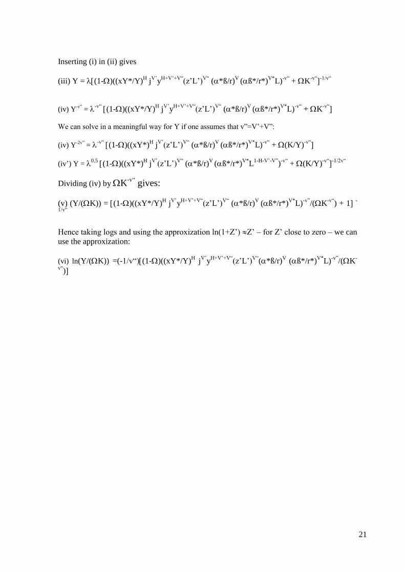
Inserting (i) in (ii) gives
(iii) Y = (1-)((xY*/Y)H j
V’y
H+V’+V“(z’L’)
V“ (*ß/r)
V (ß*/r*)
V*L)
-v“ + K
-v“
-1/v“
(iv) Y-v”
= -v“
(1-)((xY*/Y)H j
V’y
H+V’+V“(z’L’)
V“ (*ß/r)
V (ß*/r*)
V*L)
-v“ + K
-v“
We can solve in a meaningful way for Y if one assumes that v”=V’+V”:
(iv) Y-2v”
= -v“
(1-)((xY*)H j
V’(z’L’)
V“ (*ß/r)
V (ß*/r*)
V*L)
-v“ + (K/Y)
-v“
(iv’) Y = 0.5
(1-)((xY*)H j
V’(z’L’)
V“ (*ß/r)
V (ß*/r*)
V*L
1-H-V’-V”)-v“
+ (K/Y)-v“
-1/2v“
Dividing (iv) by K-v“
gives:
(v) (Y/(K)) = (1-)((xY*/Y)H j
V’y
H+V’+V“(z’L’)
V“ (*ß/r)
V (ß*/r*)
V*L)
-v”/(K
-v“) + 1
-
1/v“
Hence taking logs and using the approxization ln(1+Z’) Z’ – for Z’ close to zero – we can
use the approxization:
(vi) ln(Y/(K)) =(-1/v“)(1-)((xY*/Y)H j
V’y
H+V’+V“(z’L’)
V“(*ß/r)
V (ß*/r*)
V*L)
-v”/(K
-
v“)
Recommended