Introduction
Roland Pail, Reinhard Mayrhofer
INSTITUTE OF NAVIGATION AND SATELLITE GEODESY
GRAZ UNIVERSITY OF TECHNOLOGY
Gravity Field Simulator for the Evaluation
of Future Gravity Field Mission ConceptsS
SW
W
NW
SE
INAS
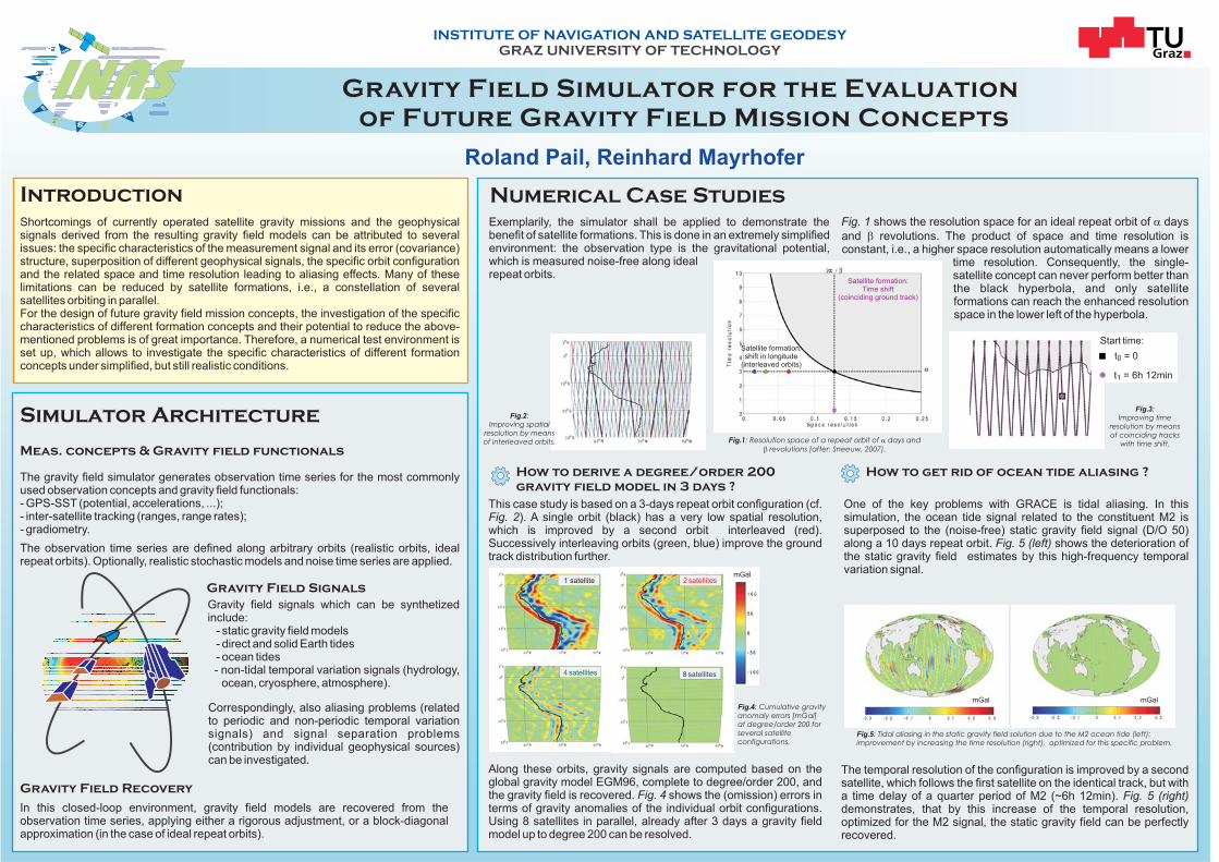
This case study is based on a 3-days repeat orbit configuration (cf.). A single orbit (black) has a very low spatial resolution,
which is improved by a second orbit interleaved (red).Successively interleaving orbits (green, blue) improve the groundtrack distribution further.
Fig. 2
Along these orbits, gravity signals are computed based on theglobal gravity model EGM96, complete to degree/order 200, andthe gravity field is recovered. shows the (omission) errors interms of gravity anomalies of the individual orbit configurations.Using 8 satellites in parallel, already after 3 days a gravity fieldmodel up to degree 200 can be resolved.
Fig. 4
Fig.1: Resolution space of a repeat orbit of days and
revolutions (after: Sneeuw, 2007).
�
�
How to get rid of ocean tide aliasing ?
Fig. 1 shows the resolution space for an ideal repeat orbit of days
and revolutions. The product of space and time resolution isconstant, i.e., a higher space resolution automatically means a lower
time resolution. Consequently, the single-satellite concept can never perform better thanthe black hyperbola, and only satelliteformations can reach the enhanced resolutionspace in the lower left of the hyperbola.
�
�
Numerical Case Studies
Exemplarily, the simulator shall be applied to demonstrate thebenefit of satellite formations. This is done in an extremely simplifiedenvironment: the observation type is the gravitational potential,which is measured noise-free along idealrepeat orbits.
How to derive a degree/order 200
gravity field model in 3 days ?
One of the key problems with GRACE is tidal aliasing. In thissimulation, the ocean tide signal related to the constituent M2 issuperposed to the (noise-free) static gravity field signal (D/O 50)along a 10 days repeat orbit. shows the deterioration ofthe static gravity field estimates by this high-frequency temporalvariation signal.
Fig. 5 (left)
Satellite formation:shift in longitude
(interleaved orbits)
Satellite formation:Time shift
(coinciding ground track)
Fig.2:Improving spatial
resolution by meansof interleaved orbits.
Fig.3:Improving time
resolution by meansof coinciding tracks
with time shift.
t = 00
t = 6h 12min1
Start time:
1 satellite
8 satellites4 satellites
2 satellites
Fig.4: Cumulative gravityanomaly errors [mGal]at degree/order 200 forseveral satelliteconfigurations.
The temporal resolution of the configuration is improved by a secondsatellite, which follows the first satellite on the identical track, but witha time delay of a quarter period of M2 (~6h 12min).demonstrates, that by this increase of the temporal resolution,optimized for the M2 signal, the static gravity field can be perfectlyrecovered.
Fig. 5 (right)
mGal
mGal mGal
Fig.5: Tidal aliasing in the static gravity field solution due to the M2 ocean tide (left);improvement by increasing the time resolution (right), optimized for this specific problem.
Shortcomings of currently operated satellite gravity missions and the geophysicalsignals derived from the resulting gravity field models can be attributed to severalissues: the specific characteristics of the measurement signal and its error (covariance)structure, superposition of different geophysical signals, the specific orbit configurationand the related space and time resolution leading to aliasing effects. Many of theselimitations can be reduced by satellite formations, i.e., a constellation of severalsatellites orbiting in parallel.For the design of future gravity field mission concepts, the investigation of the specificcharacteristics of different formation concepts and their potential to reduce the above-mentioned problems is of great importance. Therefore, a numerical test environment isset up, which allows to investigate the specific characteristics of different formationconcepts under simplified, but still realistic conditions.
Gravity field signals which can be synthetizedinclude:
- static gravity field models- direct and solid Earth tides- ocean tides- non-tidal temporal variation signals (hydrology,
ocean, cryosphere, atmosphere).
Meas. concepts & Gravity field functionals
Gravity Field Signals
Simulator Architecture
The gravity field simulator generates observation time series for the most commonlyused observation concepts and gravity field functionals:- GPS-SST (potential, accelerations, ...);- inter-satellite tracking (ranges, range rates);- gradiometry.
The observation time series are defined along arbitrary orbits (realistic orbits, idealrepeat orbits). Optionally, realistic stochastic models and noise time series are applied.
Gravity Field Recovery
In this closed-loop environment, gravity field models are recovered from theobservation time series, applying either a rigorous adjustment, or a block-diagonalapproximation (in the case of ideal repeat orbits).
Correspondingly, also aliasing problems (relatedto periodic and non-periodic temporal variationsignals) and signal separation problems(contribution by individual geophysical sources)can be investigated.
Recommended