Inflation at the Household Level
Greg Kaplan University of Chicago
and National Bureau of Economic Research
Sam Schulhofer-Wohl Federal Reserve Bank of Minneapolis
Working Paper 731 Revised June 2016
Keywords: Inflation; Heterogeneity JEL classification: D12, D30, E31
The views expressed herein are those of the authors and not necessarily those of the Federal Reserve Bank of Minneapolis or the Federal Reserve System. __________________________________________________________________________________________
Federal Reserve Bank of Minneapolis • 90 Hennepin Avenue • Minneapolis, MN 55480-0291 https://www.minneapolisfed.org/research/

Inflation at the Household Level∗
Greg Kaplan and Sam Schulhofer-Wohl
Revised June 2016
ABSTRACT
We use scanner data to estimate inflation rates at the household level. Households’ inflation ratesare remarkably heterogeneous, with an interquartile range between 6.2 to 9.0 percentage points onan annual basis. Most of the heterogeneity comes not from variation in broadly defined consumptionbundles but from variation in prices paid for the same types of goods — a source of variation thatprevious research has not measured. The entire distribution of household inflation rates shifts inparallel with aggregate inflation. Deviations from aggregate inflation exhibit only slightly negativeserial correlation within each household over time, implying that the difference between a house-hold’s price level and the aggregate price level is persistent. Together, the large cross-sectionaldispersion and low serial correlation of household-level inflation rates mean that almost all of thevariability in a household’s inflation rate over time comes from variability in household-level pricesrelative to average prices for the same goods, not from variability in the aggregate inflation rate.We provide a characterization of the stochastic process for household inflation that can be used tocalibrate models of household decisions.
Keywords: Inflation; HeterogeneityJEL classification: D12, D30, E31
∗Kaplan: University of Chicago and National Bureau of Economic Research ([email protected]).Schulhofer-Wohl: Federal Reserve Bank of Minneapolis ([email protected]). We thank Joan Giesekefor editorial assistance. The views expressed herein are those of the authors and not necessarily those of theFederal Reserve Bank of Minneapolis or the Federal Reserve System.

1. Introduction
One major objective of monetary policy in most countries is to control the inflation
rate. Policymakers typically measure inflation with an aggregate price index, such as, in
the United States, the Bureau of Economic Analysis’ price index for personal consumption
expenditures (Federal Open Market Committee, 2016). But an aggregate price index is based
on an aggregate consumption bundle and on average prices for various goods and services.
It does not necessarily correspond to the consumption bundle, prices, or inflation rate expe-
rienced by any given household. To know how changes in monetary policy and inflation will
affect households’ economic choices and well-being, we need to know how inflation behaves
at the household level.
This paper takes a first step toward an understanding of heterogeneity in inflation rates
by using scanner data on households’ purchases to characterize inflation rates at the household
level. Inflation rates can vary across households because households buy different bundles
of goods or because households pay different prices for the same goods. Previous research
on inflation heterogeneity has focused exclusively on variation in consumption bundles and
assumed that all households pay the average price for each broadly defined category of good.
By employing data from the Kilts-Nielsen Consumer Panel (KNCP), a dataset that records
the prices, quantities and specific goods purchased in 500 million transactions by about 50,000
U.S. households from 2004 through 2013, we can also consider variation in prices paid and
in the mix of goods within broad categories.1 These new sources of variation are crucial to
our results. We find that inflation at the household level is remarkably dispersed, with an
interquartile range of 6.2 to 9.0 basis points annually, about five times larger than the amount
of variation found in previous work. Almost two-thirds of the variation we measure comes
from differences in prices paid for identical goods, and about one-third from differences in the
mix of goods within broad categories; only 7 percent of the variation arises from differences
in consumption bundles defined by broad categories.
Despite the massive degree of heterogeneity, the entire distribution of household-level
1Jaravel (2015) uses the KNCP data to estimate inflation rates as a function of income but assumes thatall households in a given broad range of incomes (such as all households earning $30,000 to $100,000 per year)have the same consumption bundle and pay the same price for each good.
inflation shifts in parallel with aggregate inflation, and the central tendency of household-level
inflation closely tracks aggregate inflation.2 Households with low incomes, more household
members, or older household heads experience higher inflation on average, whereas those in
the Midwest and West experience lower inflation, but these effects are small relative to the
variance of the distribution, and observable household characteristics have little power overall
to predict household inflation rates.
The household-level inflation rates display reasonable substitution patterns in the ag-
gregate. Households substitute on average toward lower-priced goods, and the average sub-
stitution bias that results from measuring inflation with initial-period consumption bundles is
comparable in magnitude to what has been estimated for aggregate indexes such as the Con-
sumer Price Index (CPI). However, as with inflation rates themselves, substitution patterns
display a great deal of heterogeneity. Many households are observed to substitute toward
higher-priced goods, and demographics have little power to explain differences in substitu-
tion.
We also explore the evolution of households’ inflation rates over time. Deviations
from mean inflation exhibit only slightly negative serial correlation within each household
over time. As a result, inflation rates measured over time periods longer than a year are also
very heterogeneous, and the difference between a household’s price level and the aggregate
price level is quite persistent. We use our estimates to provide a simple characterization of
the stochastic process for deviations of household-level inflation from aggregate inflation. To-
gether, the low serial correlation and high cross-sectional variation of household-level inflation
imply that variation in aggregate inflation is almost irrelevant for variation in a household’s
inflation rate. In a benchmark calculation, 91 percent of the variance of a household’s infla-
tion rate comes from variation in the particular prices the household faces, and just 9 percent
from variation in the aggregate inflation rate.
Previous research on household-level heterogeneity in inflation in the United States,
such as Hobijn and Lagakos (2005) and Hobijn et al. (2009), has largely used microdata
2Neither of these results is mechanical. If the rate of increase of the prices that a particular householdpays is correlated with the household’s consumption bundle, then the mean of household inflation rates neednot match the aggregate inflation rate, and the distribution need not shift along with the aggregate.
2

from the Consumer Expenditure Survey (CEX) to measure household-specific consumption
bundles, then constructed household-level inflation rates by applying these household-specific
consumption bundles to published indexes of average prices for relatively broad categories
of goods, known as item strata. Such an analysis assumes both that all households pay the
same price for a given good (for example, a 20-ounce can of Dole pineapple chunks) and
that all households purchase the same mix of goods within each item stratum (for example,
the same mix of 20-ounce cans of Dole pineapple, other size cans of Dole pineapple, other
brands of pineapple, and other fruits within the category “canned fruits”). Relative to this
literature, our key innovation is to use the detailed price and barcode data in the KNCP to
also measure variation in the prices that households pay and the goods they choose within
item strata. We observe the barcode of each good purchased and can thus account for both
variation in the price of a specific good and variation across households in the mix of goods
purchased within item strata. We thus build on the findings of Kaplan and Menzio (2015),
who use the KNCP data to characterize variation over time and space in the prices at which
particular goods are sold. However, because the KNCP focuses on goods sold in retail outlets
— a universe that includes about 30 percent of household consumption (Kilts Center, 2013a)
— we are unable, unlike the CEX-based literature, to measure the impact of heterogeneity
in consumption of other goods and services. In particular, we cannot measure the impact of
differences in spending on education, health care, and gasoline, which Hobijn and Lagakos
(2005) found were important sources of inequality in inflation rates. Nonetheless, when we
treat the data similarly to previous research by imposing common prices on all households, we
measure a similar amount of inflation heterogeneity as in previous papers whose calculations
encompassed a broader universe of goods and services.
Our findings are also related to the growing literature on households’ and small firms’
inflation expectations. Binder (2015) and Kumar et al. (forthcoming) find that households
in the United States and small firms in New Zealand, respectively, do not have well-anchored
inflation expectations and are poorly informed about central bank policies and aggregate
inflation dynamics. One possible explanation is that if aggregate inflation is only a minor
determinant of household- or firm-level inflation, then households and firms may rationally
choose to be inattentive (Reis, 2006; Sims, 2003) to aggregate inflation and policies that
3

determine it. More broadly, the weak link between aggregate inflation and household-level
inflation may help explain the well-known long and variable lags in the impact of monetary
policy on the economy: If household-level inflation is only loosely related to aggregate infla-
tion, it may be difficult for households to detect changes in aggregate inflation, and hence
households may react weakly or at least slowly to aggregate inflation.
Since the seminal work by Lucas (1972) and Lucas (1975), macroeconomics has had a
long tradition of modeling monetary non-neutrality as arising because agents (either house-
holds or firms) have imperfect information about whether the changes they observe in nominal
variables reflect economy-wide or agent-specific shocks. More sophisticated recent descen-
dants of this literature include Angeletos and La’O (2009) and Nimark (2008). For more
than forty years, this literature has remained essentially purely theoretical, partly because
attempts to quantify the strength of the imperfect-information mechanism require some way
of disciplining the amount of information about aggregate price changes contained in indi-
vidual observations of prices. Our estimates of the stochastic process relating household-level
inflation to aggregate inflation could, in principle, be used as a first step toward empirical
quantification of these models. Although we do not take this step in this paper, our cen-
tral finding — that almost all of the variation in household-level inflation is disconnected
from movements in aggregate inflation — supports the idea that the informational frictions
embedded in these models could be substantial.
The paper proceeds as follows. Section 2 describes the data and how we construct
household-level inflation rates. Section 3 characterizes cross-sectional properties of the infla-
tion distribution. Section 4 characterizes time-series properties of household-level inflation.
Section 5 concludes.
2. Data and Estimation
This section describes the KNCP data and how we use the data to calculate inflation
rates.
A. Data
The KNCP tracks the shopping behavior of approximately 50,000 U.S. households
over the period 2004 to 2013. Households in the panel provide information about each of
4
their shopping trips using a Universal Product Code (UPC) (i.e., barcode) scanning device
provided by Nielsen. Panelists use the device to enter details about each of their shopping
trips, including the date and store where the purchases were made, and then scan the barcode
of each purchased good and enter the number of units purchased. The price of the good is
recorded in one of two ways, depending on the store where the purchase took place. If the
good was purchased at a store that Nielsen covers, the price is set automatically to the average
price of the good at the store during the week when the purchase was made. If the good was
purchased at a store that Nielsen does not cover, the price is directly entered by the panelist.
Panelists are also asked to record whether the good was purchased using one of four types
of deals: (i) store feature, (ii) store coupon, (iii) manufacturer coupon, or (iv) other deal. If
the deal involved a coupon, the panelist is prompted to input its value.
Households in the KNCP are drawn from 76 geographically dispersed markets, known
as Scantrack markets, each of which roughly corresponds to a Metropolitan Statistical Area
(MSA). Demographic data on household members are collected at the time of entry into the
panel and are then updated annually through a written survey during the fourth quarter of
each year. The collected information includes age, education, marital status, employment,
type of residence, and race. For further details on the KNCP, see Kaplan and Menzio (2015).3
We use bootstrap standard errors to account approximately for the sampling design of
the KNCP. The KNCP sample is stratified across 61 geographic areas, some of which include
multiple Scantrack markets. Nielsen replenishes the sample weekly (Kilts Center, 2013b), but
even at a quarterly frequency, there are quarters when too few new households join the sample
in some geographic strata for us to be able to resample from these households. We therefore
treat the sample as if it is replenished at an annual frequency. We resample households within
groups defined by geographic stratum and the year in which the household first appears in the
data. As recommended by Rao, Wu, and Yue (1992), we ensure that the bootstrap is unbiased
by resampling N − 1 households with replacement from a group containing N households.
When we resample a household, we include all quarterly observations from that household
3The KNCP has become an increasingly commonly used dataset for studies of prices and expenditure.Examples of recent studies that have used the KNCP include Einav, Leibtag, and Nevo (2010), Handbury(2013) and Bronnenberg et al. (2015).
5

in our bootstrap sample. Thus, our bootstrap accounts both for the geographic stratification
of the original sample and for serial correlation over time within households, for example
because of particular households’ unique purchasing patterns. However, because we do not
have access to all details of Nielsen’s sampling and weighting procedure, our bootstrap is
only approximate. In particular, we do not know whether new households are chosen purely
at random or based on observable characteristics. In addition, we cannot recompute the
sampling weights in each bootstrap sample because we do not have Nielsen’s formula for
computing the weights.
B. Calculating Household Inflation Rates
A price index measures the weighted average rate of change of some set of prices,
weighted by some consumption bundle. Aggregate price indexes use the national average
mix of consumption to define the consumption bundle. To construct household-level price
indexes, we must define household-level consumption bundles and choose a time period over
which to measure the change in prices.
We can measure the change between two dates in a household’s price for some good
only if the household buys the good on both dates. On any given day, most households do
not buy most goods — even goods that they buy relatively frequently. Therefore, although
the KNCP data record the date of each purchase, we aggregate each household’s data to a
quarterly frequency to increase the number of goods that a household is observed to buy in
multiple time periods. If a household buys the same product (defined by barcode) more than
once in a quarter, we set the household’s quarterly price for that product to the volume-
weighted average of prices that the household paid.
Many prices exhibit marked seasonality. It would be virtually impossible to seasonally
adjust the household-level price indexes because we do not observe a long time series for each
household. Therefore, we remove seasonality in price changes by constructing price indexes
at an annual frequency, comparing prices paid in quarter t and quarter t+ 4. Some residual
seasonality may remain if consumption bundles change seasonally, but in practice we observe
little seasonality in the annual price indexes we compute. To prevent mismeasured prices
from distorting our estimates, we exclude a product from the calculation for a particular
6

household at date t if the product’s price for that household increases or decreases by a factor
of more than three between t and t+ 4.
Two commonly used price indexes are the Laspeyres index, which weights price changes
between two dates by the consumption bundle at the initial date, and the Paasche index,
which weights price changes by the consumption bundle at the final date. We compute both
of these.
When we calculate a household’s inflation rate between quarters t and t + 4, we con-
sider only goods (defined by barcodes) that the household bought in both of those quarters.
To reduce sampling error, we restrict the sample to households with at least five matched
barcodes in the two quarters. (On average across all dates in the sample, 77 percent of house-
holds that make any purchase in quarter t also make some purchase in quarter t+ 4, and 72
percent buy at least five matched barcodes whose prices change by a factor no greater than
three.) Thus, let qijt be the quantity of good j bought by household i in quarter t, and let
pijt be the price paid. For each good j such that qijt > 0 and qij,t+4 > 0, we define household
i’s consumption share of good j at the initial date as
sLijt,t+4 =pijtqijt∑
j : qi`t,qij,t+4>0
pijtqijt. (1)
Similarly, we define household i’s consumption share of good j at the final date as
sPijt,t+4 =pij,t+4qij,t+4∑
j : qi`t,qij,t+4>0
pij,t+4qij,t+4
. (2)
The Laspeyres and Paasche inflation rates for household i between t and t+ 4 are then
πLit,t+4 =
∑j : qijt,
qij,t+4>0
sLijt,t+4
pij,t+4
pijt(3)
7

and
πPit,t+4 =
∑j : qijt,
qij,t+4>0
sPijt,t+4
pij,t+4
pijt, (4)
respectively. We also compute the Fisher index, which is the geometric mean of Laspeyres
and Paasche:
πFit,t+4 =
√πLit,t+4π
Pit,t+4. (5)
We compute three sets of household-level inflation indexes with prices defined at a
more aggregated level. First, we compute inflation indexes that assign to every household
the average price for each barcode. Cross-sectional variation in this index comes only from
variation in which barcodes each household buys, not from variation in the price changes for
particular barcodes. The Laspeyres index at the household level with barcode-average prices
is
πL,BCit,t+4 =
∑j : qijt,
qij,t+4>0
sLijt,t+4
pj,t+4
pjt, (6)
where pjt is the volume-weighted average price for barcode j in quarter t. The Paasche
and Fisher indexes with barcode-average prices, πP,BCi,t,t+4 and πF,BC
i,t,t+4, are defined analogously.
By comparing the indexes with household-level prices and the indexes with barcode-average
prices, we can measure how much cross-sectional variation in household inflation rates comes
from differences in which barcodes each household buys, and how much from differences in
price changes for the same barcodes.
We next compute household-level inflation indexes that, similarly to the previous
literature, account only for heterogeneity in broadly defined consumption bundles and not
for heterogeneity in prices or in the selection of specific goods within each broad category of
goods. By matching every purchase to the CPI price for the corresponding item stratum —
for example, by matching Dole canned pineapples to the canned fruit index — and assigning
to each purchase the average inflation rate for that item stratum, we can remove variation
in prices for specific goods and variation in the mix of goods within item strata, leaving
differences in how households spread their consumption across item strata as the only source
of heterogeneity. We have two possible sources for average inflation rates at the stratum level:
8

the prices observed in the KNCP and the stratum price indexes published by the BLS for the
various strata that make up the CPI. Let k(j) be the CPI category corresponding to barcode
j, and let pCPIkt be the CPI sub-index for item stratum k at date t. The Laspeyres index at
the household level with CPI prices is
πL,CPIit,t+4 =
∑j : qijt,
qij,t+4>0
sLijt,t+4
pCPIk(j),t+4
pCPIk(j),t
, (7)
and the Paasche and Fisher indexes with CPI prices, πP,CPIi,t,t+4 and πF,CPI
i,t,t+4, are defined analo-
gously.4 To produce a similar index with stratum-average prices from the KNCP, we must
first produce the analog to pCPIk,t+4/p
CPIkt with the KNCP data. The Laspeyres version of this
stratum-level inflation rate is
πL,Skt,t+4 =
∑i,j : j∈kqijt,
qij,t+4>0
qijtpj,t+4
∑i,j : j∈kqijt,
qij,t+4>0
qijtpj,t. (8)
Then the Laspeyres inflation rate at the household level with stratum-average prices is
πL,Sit,t+4 =
∑k
sLikt,t+4πL,Skt,t+4, (9)
where sLikt,t+4 is the share of stratum k in household i’s total spending at date t. The Paasche
and Fisher indexes with stratum-average prices are defined similarly.
Our household-level inflation rates are not directly comparable to published aggregate
inflation rates because our data cover only a subset of goods. We construct an aggregate
inflation rate that is comparable to our household-level indexes by measuring the aggregate
consumption bundle in our data and using this bundle to aggregate the CPI item stratum price
indexes. (We cannot make a similar comparison to the Bureau of Economic Analysis’ personal
4We calculate the quarterly value of the CPI as the average of the monthly values for the three months inthe quarter.
9

consumption expenditure index because that program does not provide prices for detailed
types of goods.) We use the Laspeyres index for this comparison because the aggregate CPI
is a Laspeyres aggregate of item stratum prices (Bureau of Labor Statistics, 2015). The
aggregate expenditure share of good j for this index is the good’s share in total spending,
counting only spending that is included in our index because it represents a household buying
the same good at both dates:
sLjt,t+4 =
∑i : qijt,
qij,t+4>0
pijtqijt
∑`
∑i : qi`t,
qi`,t+4>0
pi`tqi`t, (10)
and our aggregate inflation index is
πL,CPIt,t+4 =
∑j
sLjt,t+4
pCPIk(j),t+4
pCPIk(j),t
. (11)
The aggregate index πL,CPIt,t+4 is a version of the CPI that is based on the same set of goods
as our household-level price indexes. The price data in it are all from the CPI, and the
consumption bundle is the aggregate of the bundles used to construct our household-level
price indexes.5
The aggregate index πL,CPIt,t+4 can be rewritten as a weighted average of household-level
indexes with CPI prices:
πL,CPIt,t+4 =
∑i
xit,t+4πL,CPIit,t+4∑
i
xit,t+4
, (12)
where the weights xit,t+4 are each household i’s expenditure at date t on goods included in
the household-level price index with household-level prices:
xit,t+4 =∑
j : qijt,qij,t+4>0
pijtqijt. (13)
5Another, minor difference between our index and the published CPI is that our index is chain weighted,with new base-period weights defined at each date t, whereas the CPI uses a fixed base period.
10

Because πL,CPIt,t+4 weights households according to their spending, it is what Prais (1959) called
a plutocratic price index. The published CPI is likewise a plutocratic index because it defines
the consumption bundle based on each good’s expenditure share in aggregate spending. One
can alternatively construct democratic aggregate indexes that weight households equally, but
because our goal here is to compare household-level indexes with an analog to the published
CPI, we focus on the plutocratic index.
Table 1 compares the distribution of spending across types of goods and services in the
KNCP with the weights used to construct the published CPI. All of the data in the table are
for 2012. The first column of the table shows the weights for the CPI for urban consumers,
while the second column shows the distribution of spending in the Bureau of Labor Statistics’
Consumer Expenditure Survey (CEX) for that year; the CEX distribution differs from the
CPI weights because not all CEX households are urban. The third column of the table shows
the distribution of spending across all purchases in the KNCP data, and the fourth column
considers only the purchases that we use to construct our household inflation rates — barcodes
that a household purchases in both quarter t and quarter t+ 4, from households with at least
five matched barcodes. About 61 percent of spending in the KNCP is on food and beverages,
a share that rises to 74 percent in the matched purchases that we use to measure household
inflation. By contrast, food and beverages have only a 15 percent weight in the CPI. But
despite the heavy weight of food in the KNCP, many other types of purchases are represented,
including housekeeping supplies, pet products, and personal care items. Housing, on the other
hand, gets much less weight in our data than in the CPI, primarily because shelter, which
has a 32 percent expenditure share in the CPI, is not measured in the KNCP. Similarly, the
KNCP measures very little transportation spending. Apparel is measured in the KNCP, but
we observe no purchases of matched apparel barcodes in consecutive periods, so apparel gets
zero weight in our household inflation rates.
Figure 1 compares the aggregate index for the KNCP universe, πL,CPI , with the pub-
lished CPI and several CPI sub-indexes. The dates on the horizontal axis correspond to the
initial quarter of the one-year period over which the inflation rate is calculated. The aggre-
gate index for the KNCP data behaves similarly to the overall CPI but lags it somewhat, as
does the CPI sub-indexes for food at home. Unsurprisingly, given the large share of food at
11

Table 1: Percentage distribution of spending across categories in different datasets, 2012.
KNCP
CPI-U CEX all spending 5+ matched UPCs
Food and beverages 15.26 16.03 61.22 74.38Food 14.31 15.00 58.08 67.61
Food at home 8.60 8.91 53.87 64.77Cereals and bakery products 1.23 1.22 7.71 9.10
Cereals and cereal products 0.47 0.41 2.91 3.25Bakery products 0.76 0.81 4.80 5.86
Meats, poultry, fish, and eggs 1.96 1.94 7.53 6.35Meats, poultry, and fish 1.84 1.82 6.98 4.93Eggs 0.11 0.12 0.55 1.42
Dairy and related products 0.91 0.95 7.92 13.15Fruits and vegetables 1.29 1.66 7.36 6.90Nonalcoholic beverages, beverage materials 0.94 0.84 6.85 13.52Other food at home 2.28 2.30 14.84 15.75
Sugar and sweets 0.31 0.33 2.95 3.05Fats and oils 0.26 0.26 1.58 2.40Other foods 1.71 1.70 10.31 10.30
Food away from home 5.71 6.09 4.22 2.83Alcoholic beverages 0.95 1.03 3.13 6.78
Housing 41.02 35.63 9.03 5.11Shelter 31.68 22.52 - -Fuels and utilities 5.30 5.49 0.08 0.08Household furnishings and operations 4.04 7.62 8.95 5.04
Window and floor coverings and other linens 0.27 0.32 - -Furniture and bedding 0.71 0.89 - -Appliances 0.29 0.67 1.17 0.09Other household equipment and furnishings 0.48 - 1.07 0.14Tools, hardware, outdoor equipment, supplies 0.68 - 1.09 0.21Housekeeping supplies 0.89 1.39 5.62 4.59Household operations 0.73 2.64 - -
Apparel 3.56 3.95 8.40 -Transportation 16.85 20.48 0.22 0.14
Private transportation 15.66 19.25 0.22 0.14Public transportation 1.19 1.23 - -
Medical care 7.16 8.10 6.92 4.85Recreation 5.99 6.18 6.57 5.85
Video and audio 1.90 2.23 2.11 0.47Pets, pet products and services 1.10 - 4.27 5.37Sporting goods 0.46 - - -Photography 0.11 - 0.16 0.01Other recreational goods 0.45 - 0.02 -Other recreation services 1.75 - - -Recreational reading materials 0.23 - - -
Education and communication 6.78 5.57 - -Other goods and services 3.38 4.07 7.64 9.67
Tobacco and smoking products 0.81 0.76 1.87 6.46Personal care 2.57 1.43 4.47 2.66
Subcategories are not exhaustive and do not necessarily add up to higher-level categories.
12

−3
03
69
perc
enta
gepo
ints
2004 2005 2006 2007 2008 2009 2010 2011 2012
CPI CPI food at home CPI ex energyKNCP aggregate +/− 2 s.e.
Figure 1: Aggregate inflation rates.CPI inflation rates computed as annual percentage change in quarterly average of monthly index
values. Inflation rate plotted for each quarter is the change in price index from that quarter to the
quarter one year later. Vertical bars show an interval of ± 2 bootstrap standard errors around each
point estimate. Source for CPI data: Bureau of Labor Statistics.
home in the KNCP data, our index moves closely with the CPI for food at home, though our
index is somewhat less volatile. The overweighting of food offsets the absence of energy in
our data, so that our index’s volatility is similar to that of the overall CPI and substantially
greater than the volatility of the CPI excluding energy. Over the period we study, our aggre-
gate inflation rate averages 2.6 percent with a standard deviation of 1.9 percentage points,
compared with a mean of 2.4 percent and standard deviation of 1.5 percentage points for the
published CPI, and a mean of 2.6 percent and standard deviation of 2.4 percentage points for
the food-at-home sub-index. Our index is precisely estimated; the bootstrap standard errors
average 2 basis points.
Both when we compute the aggregate consumption bundle and when we compute
household price indexes with CPI prices or barcode-level prices, we use only those specific
goods — defined by barcodes — that each household purchases at both dates. Thus, in all
of our indexes, we measure inflation for the subset of goods that households buy repeatedly.
This inflation rate may differ from an inflation rate that includes goods bought less frequently,
but we have no way to compute the latter rate at the household level.
The foregoing analysis considers only differences in the categories of goods covered in
13

−6
−4
−2
02
46
perc
enta
ge p
oint
s
2004 2005 2006 2007 2008 2009 2010 2011 2012
10th, 90th percentiles
25th, 75th percentiles
median
mean
(a) distribution of deviations between KNCP and CPI stratum inflation rates−
20
24
68
perc
enta
ge p
oint
s
2004 2005 2006 2007 2008 2009 2010 2011 2012
KNCP prices CPI prices
(b) aggregate inflation rates computed with KNCP and CPI prices
Figure 2: Comparison of KNCP and CPI inflation rates at the item stratum level.Panel (a) shows distribution across item strata of difference between inflation rate computed with
KNCP data and that published for the CPI. Panel (b) shows average inflation rates across all item
strata using KNCP data and using published CPI indexes, weighted by distribution of spending
in the KNCP. CPI inflation rates computed as annual percentage change in quarterly average of
monthly index values. Inflation rate plotted for each quarter is the change in price index from that
quarter to the quarter one year later. 14

the KNCP versus the CPI, applying the same CPI prices to both datasets. (Recall that we
use CPI prices to compute the KNCP aggregate inflation index, πL,CPI .) However, when we
compute household-level inflation rates, we will use price data from the KNCP. In principle,
the prices recorded in the KNCP could differ from those recorded in the CPI for similar goods.
To assess this concern, we map each barcode in the KNCP to a CPI item stratum and compute
inflation rates in the KNCP for each item stratum.6 Figure 2 shows two ways of comparing
the resulting item stratum inflation rates in the KNCP with the corresponding published item
stratum inflation rates for the CPI. In the upper panel, we show the distribution across item
strata of the difference between the KNCP inflation rate and the published CPI inflation rate.
The mean and median differences are small, and in most quarters, the discrepancy is no more
than 1 percentage point for roughly half of the item strata. However, some item strata have
substantially larger discrepancies. The lower panel of the figure aggregates the item strata
inflation rates from the KNCP and the CPI to produce aggregate inflation rates, weighting
each item stratum by total expenditure on that stratum in the KNCP. The aggregate inflation
rate using KNCP prices is almost identical to that using CPI prices. Thus, on average, the
prices recorded in the KNCP reflect the same trends as the prices recorded in the CPI.
3. The Cross-Sectional Distribution of Inflation Rates
Figure 3 shows the distributions of household-level inflation rates for a typical pe-
riod, the fourth quarter of 2004 to the fourth quarter of 2005, calculated with Laspeyres
indexes. In each panel, a kernel density estimate of the distribution of household-level infla-
tion rates with household-level prices is superimposed on estimates of the distributions of the
household-level rates with barcode-average prices, with stratum-average prices, and with CPI
prices. Household-level inflation rates with household-level prices are remarkably dispersed.
The interquartile range of annual inflation rates is 6.7 percentage points, and the difference
between the 10th and 90th percentiles is 14.8 percentage points. (The distributions of the
Fisher and Paasche indexes are similar and are shown in the web appendix.) For legibility,
the plots run from the 1st to 99th percentiles of the distribution of household-level inflation
6We compute these inflation rates using the Laspeyres index and the volume-weighted average observedprice for each barcode at each date.
15

0.2
.4.6
.8de
nsity
−20 −10 0 10 20household inflation rate (%)
(a) Laspeyres indexes, 5+ barcodes0
.2.4
.6.8
dens
ity
−20 −10 0 10 20household inflation rate (%)
(b) Laspeyres indexes, 25+ barcodes
0.2
.4.6
.8de
nsity
−20 −10 0 10 20household inflation rate (%)
(c) Laspeyres indexes, 30%+ matched spending
household−level prices barcode−average prices
stratum−average prices CPI prices
Figure 3: Distributions of household-level inflation rates from fourth quarter of 2004 to fourthquarter of 2005.Kernel density estimates using Epanechnikov kernel. Bandwidth is 0.05 percentage point for inflation
rates with household-level and barcode-average prices and 0.005 percentage point for inflation rates
with CPI prices. Data on 23,635 households with matched consumption in 2004q4 and 2005q4.
Plots truncated at 1st and 99th percentiles of distribution of inflation rates with household-level
prices. 16

with household-level prices, but a few households have much more extreme inflation rates;
the smallest observed inflation rate at the household level with the Laspeyres index in the
fourth quarter of 2004 was −43 percent, and the largest was 102 percent.
The vast majority of the cross-sectional variation in household-level price indexes
comes from cross-sectional dispersion in prices paid for goods within an item stratum, not
variation in the allocation of expenditure to item strata. The variance of the index with
CPI prices is 2.5 percent of the variance of the index with household-level prices,7 and the
interquartile range is just 0.95 percentage point. The inflation rates with stratum-average
KNCP prices are slightly more dispersed, with an interquartile range of 1.25 percentage point
and a variance that is 9.8 percent of the variance of the index with household-level prices.
Relative to the CPI prices, stratum-average prices in the KNCP are likely to be a noisy
measure of the true stratum-level price indexes. As a result, the household-level inflation rates
with stratum-average prices are likely to overstate the true amount of variation attributable
to allocation of expenditure across item strata. Therefore, in the remainder of the analysis,
we use CPI prices to assess the amount of variation due to the allocation of expenditure
across item strata.
Differences in the barcodes that households buy within item strata and differences in
the prices that households pay for particular barcodes are both important sources of variation
in household-level price indexes. The variance of the Laspeyres index with barcode-average
prices is 30.6 percent of the variance of the index with household-level prices, implying that
66.9 percent of the variation in the index with household-level prices comes from variation
across households in the prices paid for given barcodes, 30.6 percent from variation in the
choice of barcodes within item strata, and 2.5 percent from variation in the mix of consump-
tion across item strata.
The heterogeneity in inflation rates is not driven by households for which we can
match only a few barcodes across quarters. The distributions for households with at least 25
matched barcodes, shown in the middle panel of Figure 3, are almost as dispersed as those for
7We compute all variances on the subset of observations that fall between the 1st and 99th percentiles ofthe distribution of the index with household-level prices, to remove some extreme cases that would inflatethe variance with household-level prices.
17

the baseline group of households with at least five matched barcodes, shown in the top panel.
Among households with at least 25 matched barcodes, the interquartile range of Laspeyres
inflation rates with household prices is 5.8 percentage points, the difference between the 10th
and 90th percentiles is 12.1 percentage points, the variance of the index with CPI prices is 2.7
percent of the variance of the index with household-level prices, and the variance of the index
with barcode-average prices is 31.0 percent of the variance of the index with household-level
prices.
Spending on matched barcodes is only a minority of most households’ spending. For
the median household, across all quarters, 21 percent of spending is on matched barcodes,
and for three-quarters of households, less than 30 percent of spending is on matched barcodes.
However, the heterogeneity in inflation rates is not driven by households for which especially
little spending is on matched barcodes. The distributions of inflation rates for the one-fourth
of households that devote at least 30 percent of their spending to matched barcodes, shown
in the bottom panel of Figure 3, show similar dispersion to those for all households.
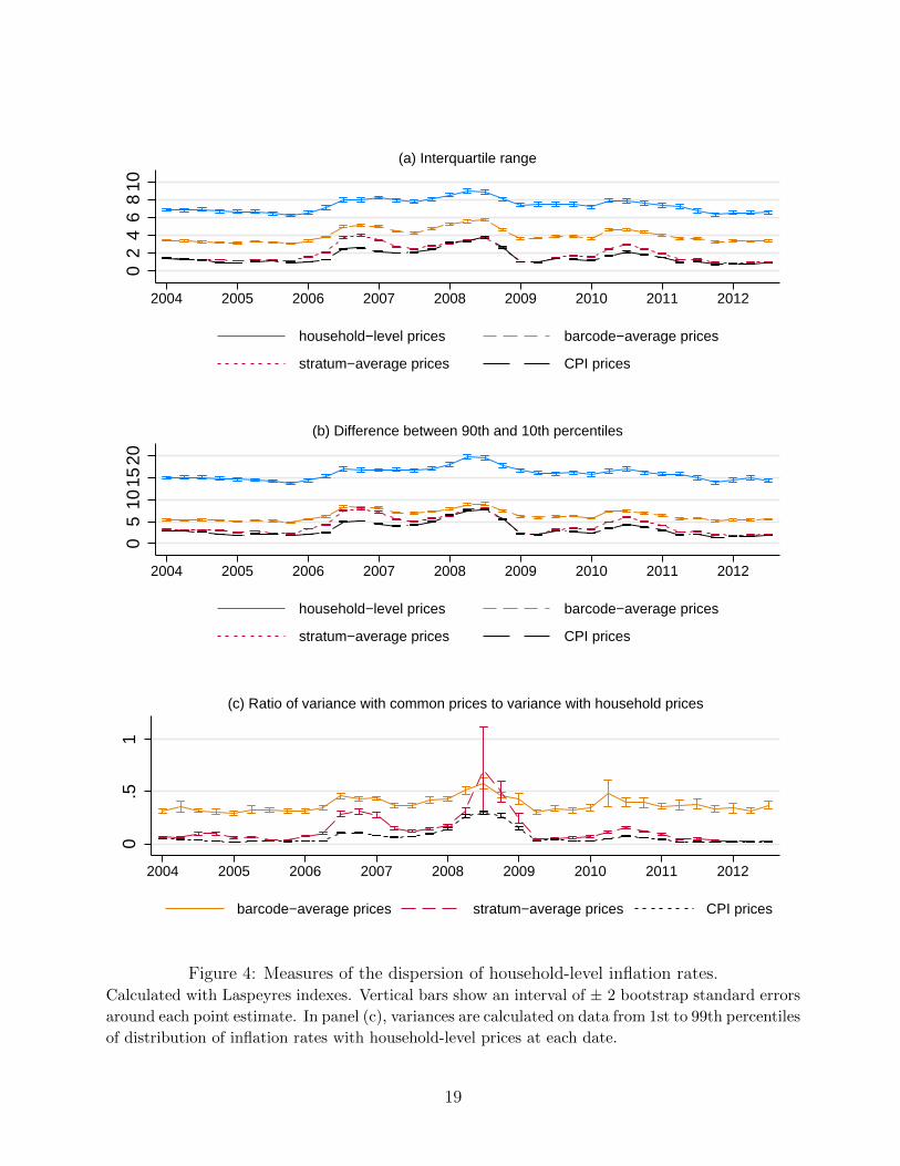
Figure 4 examines how the dispersion of household-level inflation rates evolves over
time. The graphs show results calculated from Laspeyres indexes, but graphs based on
Paasche and Fisher indexes, shown in the web appendix, are almost identical. Table 2
summarizes the dispersion measures from all three indexes. The patterns observed in the
fourth quarter of 2004 are quite typical. Household-level inflation rates with household-level
prices are enormously dispersed, with interquartile ranges of 6.2 to 9.0 percentage points
using the Laspeyres index, and much more dispersed than household-level inflation rates
with barcode-average, stratum-average or CPI prices. The bootstrap standard errors show
that the amount of dispersion is precisely estimated at each date.
On the whole, the inflation inequality we measure with CPI prices is similar to what
has been reported in previous literature that uses a wider universe of goods and services and
imposes CPI prices on all households. For example, Hobijn et al. (2009) found a gap of 1
to 3 percentage points between the 10th and 90th percentiles. But our results show that
assuming all households face the same prices and buy the same mix of goods within CPI item
strata misses most of the heterogeneity in inflation rates. The gap between the 10th and 90th
percentiles is nearly twice as large when we use barcode-average prices, allowing the mix of
18
02
46
810
2004 2005 2006 2007 2008 2009 2010 2011 2012
household−level prices barcode−average prices
stratum−average prices CPI prices
(a) Interquartile range
05
1015
20
2004 2005 2006 2007 2008 2009 2010 2011 2012
household−level prices barcode−average prices
stratum−average prices CPI prices
(b) Difference between 90th and 10th percentiles
0.5
1
2004 2005 2006 2007 2008 2009 2010 2011 2012
barcode−average prices stratum−average prices CPI prices
(c) Ratio of variance with common prices to variance with household prices
Figure 4: Measures of the dispersion of household-level inflation rates.Calculated with Laspeyres indexes. Vertical bars show an interval of ± 2 bootstrap standard errors
around each point estimate. In panel (c), variances are calculated on data from 1st to 99th percentiles
of distribution of inflation rates with household-level prices at each date.
19

Table 2: Measures of the dispersion of household-level inflation rates.
mean s.d. min maxA. Interquartile rangeHousehold-level prices:
Laspeyres 7.33 0.74 6.23 8.99Fisher 7.13 0.72 6.12 8.92Paasche 7.37 0.76 6.34 9.18
Barcode-average prices:Laspeyres 3.99 0.77 3.06 5.73Fisher 3.87 0.75 2.95 5.68Paasche 3.98 0.76 3.03 5.81
Stratum-average prices:Laspeyres 1.96 0.95 0.89 3.96Fisher 1.83 0.88 0.91 3.84Paasche 1.95 0.92 0.92 3.92
CPI prices:Laspeyres 1.61 0.80 0.71 3.77Fisher 1.57 0.77 0.70 3.53Paasche 1.62 0.78 0.71 3.42
B. Difference between 90th and 10th percentilesHousehold-level prices:
Laspeyres 15.87 1.44 13.67 19.74Fisher 15.32 1.36 13.27 18.84Paasche 15.83 1.38 13.76 19.48
Barcode-average prices:Laspeyres 6.39 1.18 4.85 8.94Fisher 6.15 1.14 4.70 8.69Paasche 6.31 1.14 4.84 8.82
Stratum-average prices:Laspeyres 4.12 1.93 1.93 7.92Fisher 3.78 1.75 1.92 7.99Paasche 4.07 1.89 1.97 8.41
CPI prices:Laspeyres 3.30 1.66 1.41 7.69Fisher 3.21 1.58 1.38 7.17Paasche 3.33 1.61 1.44 7.07
C. Ratio of variance with common prices to variancewith household pricesBarcode-average prices:
Laspeyres 0.38 0.07 0.29 0.58Fisher 0.37 0.07 0.29 0.58Paasche 0.37 0.07 0.30 0.59
Stratum-average prices:Laspeyres 0.14 0.15 0.03 0.71Fisher 0.10 0.09 0.02 0.41Paasche 0.12 0.11 0.03 0.44
CPI prices:Laspeyres 0.07 0.07 0.01 0.30Fisher 0.07 0.08 0.01 0.30Paasche 0.07 0.08 0.01 0.30
Averages from 2004q1 through 2012q3 of dispersion measures for each date.
20
−10
−5
05
1015
perc
enta
ge p
oint
s
2004 2005 2006 2007 2008 2009 2010 2011 2012
10th, 90th percentiles25th, 75th percentiles
medianmean
aggregate index
Figure 5: Evolution of the distribution of household inflation rates with household-level prices.Calculated with Laspeyres indexes. Mean is calculated on data from 1st to 99th percentiles of
distribution of inflation rates at each date.
goods within item strata to vary across households, as when we use CPI prices. And if we
also allow different households to pay different prices for the same barcode, the gap between
the 10th and 90th percentiles is five times larger than when we use CPI prices.
The bottom panel of Figure 4 shows that in most years, the variance of inflation
rates with CPI prices is only a few percent of the variance of inflation rates with household-
level prices. However, in 2008, at the height of the Great Recession, the variance with CPI
prices reaches 30 percent of the variance with household-level prices, as the sharp shift in the
relative price of food at home, shown in Figure 1, makes heterogeneity in broadly defined
consumption bundles more important. The variance of inflation rates with barcode-average
prices is typically about one-third of the variance with household-level prices, but rises in
2008. Table 2 shows that dispersion measured with the Fisher index is slightly lower than
that measured with Laspeyres and Paasche indexes.
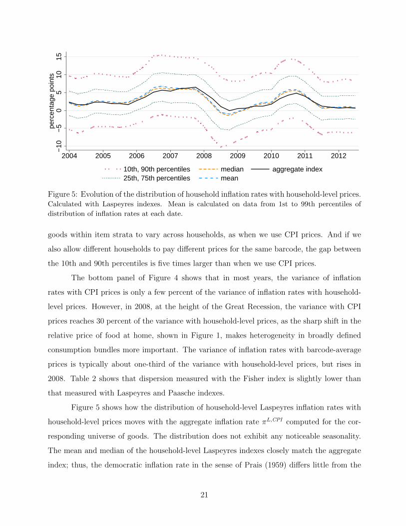
Figure 5 shows how the distribution of household-level Laspeyres inflation rates with
household-level prices moves with the aggregate inflation rate πL,CPI computed for the cor-
responding universe of goods. The distribution does not exhibit any noticeable seasonality.
The mean and median of the household-level Laspeyres indexes closely match the aggregate
index; thus, the democratic inflation rate in the sense of Prais (1959) differs little from the
21
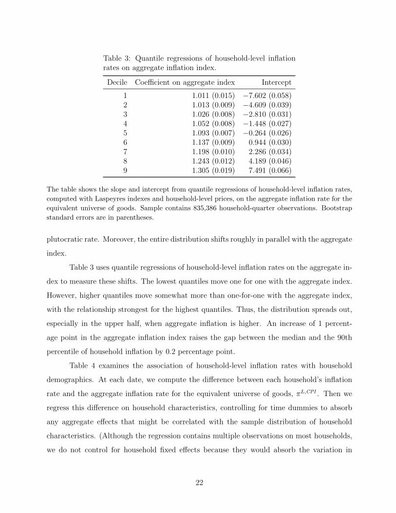
Table 3: Quantile regressions of household-level inflationrates on aggregate inflation index.
Decile Coefficient on aggregate index Intercept
1 1.011 (0.015) −7.602 (0.058)2 1.013 (0.009) −4.609 (0.039)3 1.026 (0.008) −2.810 (0.031)4 1.052 (0.008) −1.448 (0.027)5 1.093 (0.007) −0.264 (0.026)6 1.137 (0.009) 0.944 (0.030)7 1.198 (0.010) 2.286 (0.034)8 1.243 (0.012) 4.189 (0.046)9 1.305 (0.019) 7.491 (0.066)
The table shows the slope and intercept from quantile regressions of household-level inflation rates,
computed with Laspeyres indexes and household-level prices, on the aggregate inflation rate for the
equivalent universe of goods. Sample contains 835,386 household-quarter observations. Bootstrap
standard errors are in parentheses.
plutocratic rate. Moreover, the entire distribution shifts roughly in parallel with the aggregate
index.
Table 3 uses quantile regressions of household-level inflation rates on the aggregate in-
dex to measure these shifts. The lowest quantiles move one for one with the aggregate index.
However, higher quantiles move somewhat more than one-for-one with the aggregate index,
with the relationship strongest for the highest quantiles. Thus, the distribution spreads out,
especially in the upper half, when aggregate inflation is higher. An increase of 1 percent-
age point in the aggregate inflation index raises the gap between the median and the 90th
percentile of household inflation by 0.2 percentage point.
Table 4 examines the association of household-level inflation rates with household
demographics. At each date, we compute the difference between each household’s inflation
rate and the aggregate inflation rate for the equivalent universe of goods, πL,CPI . Then we
regress this difference on household characteristics, controlling for time dummies to absorb
any aggregate effects that might be correlated with the sample distribution of household
characteristics. (Although the regression contains multiple observations on most households,
we do not control for household fixed effects because they would absorb the variation in
22

household characteristics, which are mostly time invariant.) The first two columns compute
household-level inflation rates with household-level prices and the Laspeyres index, estimating
the coefficients first with ordinary least squares regression and then with median regression,
which is robust to outliers in the inflation distribution.The third and fourth columns compute
household-level inflation rates with barcode-average and CPI prices, respectively, estimating
the coefficients with median regression in both cases.
The results with household-level prices show several significant associations between
demographics and household-inflation. Low-income households experience higher inflation.
According to the median regression, the median annual inflation rate is 0.6 percentage point
higher for a household with income below $20,000, compared with a household with income
of at least $100,000. The difference is even larger for mean inflation rates, measured with the
OLS regression. The inflation rate also is nearly half a percentage point lower for households
in the West than in the East, and almost 0.2 percentage point lower in the Midwest than in the
East. Larger households have higher inflation rates; the median inflation rate is one-fourth of
a percentage point higher for a family of two adults and two children than for a single adult.
In both the OLS and median regressions, inflation rates with household-level prices are higher
for households whose heads are older. Differences by race are not statistically significant.
The results with barcode-average and CPI prices show similar correlations, except
that the magnitude of the coefficients typically becomes smaller as prices are computed at
higher levels of aggregation. For example, the difference in median inflation rates between the
lowest and highest income groups is 0.1 percentage point with CPI prices and 0.4 percentage
point with barcode-average prices, compared with 0.6 percentage point with household-level
prices. The coefficients on age categories likewise shrink as prices are aggregated, as do the
coefficients on region and household size. Thus, measures of household-level inflation that
use aggregated prices may underestimate the differences in inflation rates across demographic
groups. However, education is an exception to this pattern, with barcode-average prices
producing larger coefficients than household-level prices.
Although Table 4 reveals several statistically and economically significant associations
of household inflation with observables, these effects are small relative to the total amount of
heterogeneity. For example, moving from the bottom to the top of the age distribution raises
23

Table 4: Regressions of household-level inflation rates on household demographics.
Deviation of household inflation from aggregate inflation
(1) OLS, (2) Median, (3) Median, (4) Median,household prices household prices barcode prices CPI prices
coeff. std. err. coeff. std. err. coeff. std. err. coeff. std. err.
household income$20,000–$39,999 -0.206 (0.055) -0.126 (0.039) -0.093 (0.025) -0.061 (0.010)$40,000–$59,999 -0.420 (0.052) -0.257 (0.041) -0.185 (0.027) -0.077 (0.011)$60,000–$99,999 -0.587 (0.059) -0.468 (0.045) -0.267 (0.028) -0.099 (0.013)≥$100,000 -0.731 (0.065) -0.597 (0.050) -0.404 (0.035) -0.124 (0.013)
average age of household head(s)30–39 0.384 (0.205) 0.244 (0.145) 0.160 (0.089) 0.066 (0.028)40–49 0.451 (0.203) 0.297 (0.137) 0.218 (0.090) 0.085 (0.025)50–59 0.511 (0.206) 0.362 (0.137) 0.262 (0.090) 0.111 (0.027)60–69 0.552 (0.199) 0.430 (0.139) 0.287 (0.088) 0.104 (0.027)≥70 0.552 (0.203) 0.457 (0.140) 0.276 (0.090) 0.065 (0.027)
highest education of household head(s)high school diploma -0.064 (0.127) -0.029 (0.108) -0.120 (0.054) -0.062 (0.023)some college -0.138 (0.127) -0.102 (0.107) -0.162 (0.054) -0.092 (0.024)bachelor’s degree -0.251 (0.128) -0.163 (0.110) -0.238 (0.058) -0.125 (0.025)graduate degree -0.285 (0.139) -0.137 (0.118) -0.267 (0.063) -0.141 (0.025)
Census regionMidwest -0.179 (0.049) -0.175 (0.040) -0.029 (0.025) -0.025 (0.009)South -0.140 (0.046) -0.063 (0.033) 0.041 (0.023) 0.006 (0.008)West -0.517 (0.054) -0.429 (0.046) -0.254 (0.027) -0.039 (0.011)
# household members 0.089 (0.022) 0.110 (0.018) 0.058 (0.012) 0.026 (0.005)has children -0.115 (0.118) 0.074 (0.094) -0.153 (0.066) 0.048 (0.024)has children × 0.002 (0.034) -0.033 (0.029) 0.012 (0.020) -0.029 (0.007)
# household membersblack 0.058 (0.064) 0.063 (0.049) -0.019 (0.027) -0.061 (0.011)Asian -0.074 (0.156) -0.089 (0.125) -0.013 (0.070) -0.010 (0.019)other nonwhite -0.033 (0.087) -0.025 (0.067) 0.053 (0.045) 0.007 (0.017)Hispanic -0.068 (0.068) -0.085 (0.056) -0.092 (0.036) -0.010 (0.013)
R2 0.012 - - -R2 (time dummies only) 0.009 - - -N 835,386 835,386 835,386 835,386
The dependent variable is the difference between the household inflation rate and the aggregate
inflation rate for the equivalent universe of goods. Bootstrap standard errors are in parentheses. In
columns (1) and (2), the household inflation rate is computed with household-level prices; column
(3) uses barcode-average prices, and column (4) uses CPI prices. All columns use Laspeyres indexes.
Column (1) shows results from ordinary least squares regression, and columns (2), (3), and (4) from
median regression. Regressions include time dummy variables. Omitted categories of categorical
variables are: income less than $20,000; white; non-Hispanic; heads’ average age less than 30; heads’
highest education less than high school diploma; Northeast region.
24
−.5
−.2
50
.25
.5pe
rcen
tage
poi
nts
2004 2005 2006 2007 2008 2009 2010 2011 2012
Laspeyres Paasche
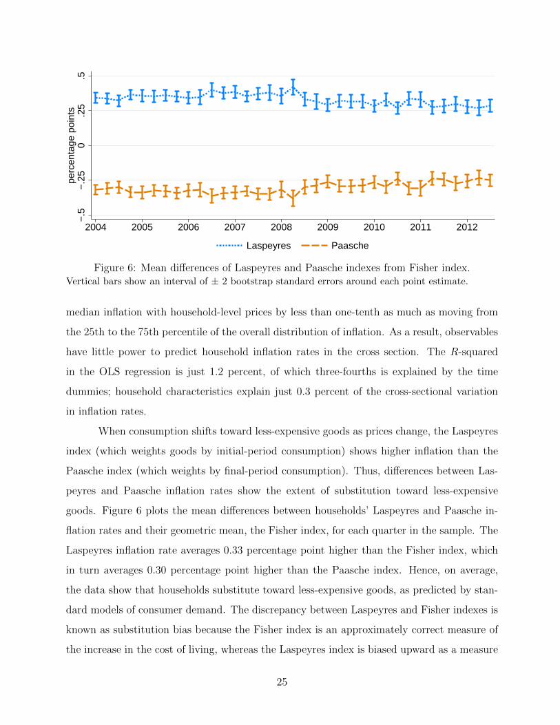
Figure 6: Mean differences of Laspeyres and Paasche indexes from Fisher index.Vertical bars show an interval of ± 2 bootstrap standard errors around each point estimate.
median inflation with household-level prices by less than one-tenth as much as moving from
the 25th to the 75th percentile of the overall distribution of inflation. As a result, observables
have little power to predict household inflation rates in the cross section. The R-squared
in the OLS regression is just 1.2 percent, of which three-fourths is explained by the time
dummies; household characteristics explain just 0.3 percent of the cross-sectional variation
in inflation rates.
When consumption shifts toward less-expensive goods as prices change, the Laspeyres
index (which weights goods by initial-period consumption) shows higher inflation than the
Paasche index (which weights by final-period consumption). Thus, differences between Las-
peyres and Paasche inflation rates show the extent of substitution toward less-expensive
goods. Figure 6 plots the mean differences between households’ Laspeyres and Paasche in-
flation rates and their geometric mean, the Fisher index, for each quarter in the sample. The
Laspeyres inflation rate averages 0.33 percentage point higher than the Fisher index, which
in turn averages 0.30 percentage point higher than the Paasche index. Hence, on average,
the data show that households substitute toward less-expensive goods, as predicted by stan-
dard models of consumer demand. The discrepancy between Laspeyres and Fisher indexes is
known as substitution bias because the Fisher index is an approximately correct measure of
the increase in the cost of living, whereas the Laspeyres index is biased upward as a measure
25

0.0
5.1
.15
.2de
nsity
−10 −5 0 5 10 15difference between household Laspeyres and Paasche inflation rates (%)
Figure 7: Distribution of household-level differences between Laspeyres and Paasche indexesfrom fourth quarter of 2004 to fourth quarter of 2005.Kernel density estimates using Epanechnikov kernel. Bandwidth is 0.05 percentage point. Data
on 23,635 households with matched consumption in 2004q4 and 2005q4. Plot truncated at 1st and
99th percentiles of distribution of inflation rates with household-level prices.
of the cost of living because it ignores substitution toward lower-priced goods. The 0.33
percentage point average substitution bias in our household-level inflation rates is similar to
typical estimates of substitution bias in aggregate data, such as the Boskin Commission’s
estimate of a 0.4 percentage point substitution bias in the CPI (Boskin et al., 1996, Table 3).
The average substitution patterns mask a great deal of heterogeneity. Figure 7 shows
the distribution of the difference between the Laspeyres and Paasche indexes for each house-
hold, πLit,t+4 − πP
it,t+4, for a typical period, the fourth quarter of 2004 to the fourth quarter
of 2005. Although the Paasche index measures a lower inflation rate than the Laspeyres
index for the average household, this relationship is far from uniform. Slightly more than 40
percent of households fail to substitute in the expected direction and have a higher Paasche
index than Laspeyres index.
Table 5 measures the relationship between household demographics and substitution
patterns. We use ordinary least squares and median regressions to examine the association
of the Laspeyres-Paasche difference with household demographics, and a linear probability
model to examine how demographics relate to the probability that a household’s Laspeyres
inflation rate is greater than its Paasche inflation rate. These regressions use the data for
26
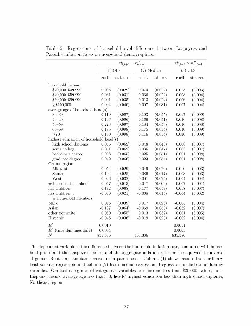
Table 5: Regressions of household-level difference between Laspeyres andPaasche inflation rates on household demographics.
πLit,t+4 − πP
it,t+4 πLit,t+4 > πP
it,t+4
(1) OLS (2) Median (3) OLS
coeff. std. err. coeff. std. err. coeff. std. err.
household income$20,000–$39,999 0.095 (0.029) 0.074 (0.022) 0.013 (0.003)$40,000–$59,999 0.031 (0.031) 0.036 (0.022) 0.008 (0.004)$60,000–$99,999 0.001 (0.035) 0.013 (0.024) 0.006 (0.004)≥$100,000 -0.004 (0.040) 0.007 (0.031) 0.007 (0.004)
average age of household head(s)30–39 0.119 (0.097) 0.103 (0.055) 0.017 (0.009)40–49 0.196 (0.096) 0.166 (0.051) 0.030 (0.008)50–59 0.228 (0.097) 0.184 (0.053) 0.030 (0.008)60–69 0.195 (0.098) 0.175 (0.054) 0.030 (0.009)≥70 0.100 (0.098) 0.116 (0.054) 0.020 (0.009)
highest education of household head(s)high school diploma 0.056 (0.062) 0.048 (0.048) 0.008 (0.007)some college 0.051 (0.062) 0.036 (0.047) 0.003 (0.007)bachelor’s degree 0.008 (0.065) 0.025 (0.051) 0.001 (0.008)graduate degree 0.042 (0.066) 0.023 (0.054) 0.001 (0.008)
Census regionMidwest 0.054 (0.029) 0.049 (0.020) 0.010 (0.003)South -0.104 (0.025) -0.086 (0.017) -0.003 (0.003)West 0.026 (0.032) -0.001 (0.024) 0.004 (0.004)
# household members 0.047 (0.013) 0.047 (0.009) 0.007 (0.001)has children 0.132 (0.068) 0.177 (0.053) 0.018 (0.007)has children × -0.036 (0.021) -0.038 (0.015) -0.004 (0.002)
# household membersblack 0.046 (0.039) 0.017 (0.025) -0.005 (0.004)Asian -0.137 (0.064) -0.069 (0.053) -0.022 (0.007)other nonwhite 0.050 (0.055) 0.013 (0.032) 0.001 (0.005)Hispanic -0.046 (0.036) -0.019 (0.023) -0.002 (0.004)
R2 0.0010 0.0011R2 (time dummies only) 0.0004 0.0003N 835,386 835,386 835,386
The dependent variable is the difference between the household inflation rate, computed with house-
hold prices and the Laspeyres index, and the aggregate inflation rate for the equivalent universe
of goods. Bootstrap standard errors are in parentheses. Column (1) shows results from ordinary
least squares regression, and column (2) from median regression. Regressions include time dummy
variables. Omitted categories of categorical variables are: income less than $20,000; white; non-
Hispanic; heads’ average age less than 30; heads’ highest education less than high school diploma;
Northeast region.
27

all quarters and control for time effects. The largest effects are found for age, income, and
household size. Households with heads between ages 40 and 70 have an average Laspeyres-
Paasche difference about 0.2 percentage point larger than households with heads between
ages 20 and 29; this is substantial relative to the mean difference of 0.6 percentage point.
Households with children also show stronger substitution, as do those with relatively low, but
not the lowest, incomes. Nonetheless, as with household-level inflation rates themselves, the
low R-squared in the regressions shows that demographics have almost no power to explain
differences between households’ Laspeyres and Paasche inflation rates.
4. Time-Series Properties of Household-Level Inflation
The long-run impact of heterogeneous inflation rates on households’ welfare depends
on whether the heterogeneity is persistent or whether a household that experiences high
inflation in one year tends to experience an offsetting low inflation rate in the next year.
Figure 8 examines this persistence for a particular pair of years, 2004–2005 and 2005–
2006. The figure shows the distributions of household inflation rates in 2004–2005 and in
2005–2006, as well as the distribution of the annualized inflation rate that each household
experienced over the two-year period from 2004 to 2006. The distributions of inflation rates
for the two one-year periods are similar, whereas the annualized two-year inflation rates are
somewhat less dispersed but still very heterogeneous. Among the households with inflation
rates measured in both one-year periods, the interquartile range of the Laspeyres inflation
rates with household prices is 6.57 percentage points in 2004–2005, 6.10 percentage points in
2005–2006, and 4.29 percentage points for annualized inflation rates over 2004–2006. Results
are similar for Fisher and Paasche indexes, shown in the online appendix. Inflation rates with
barcode-average, stratum-average, and CPI prices are likewise quite persistent. Thus, even
over horizons longer than a year, households experience markedly different inflation rates.
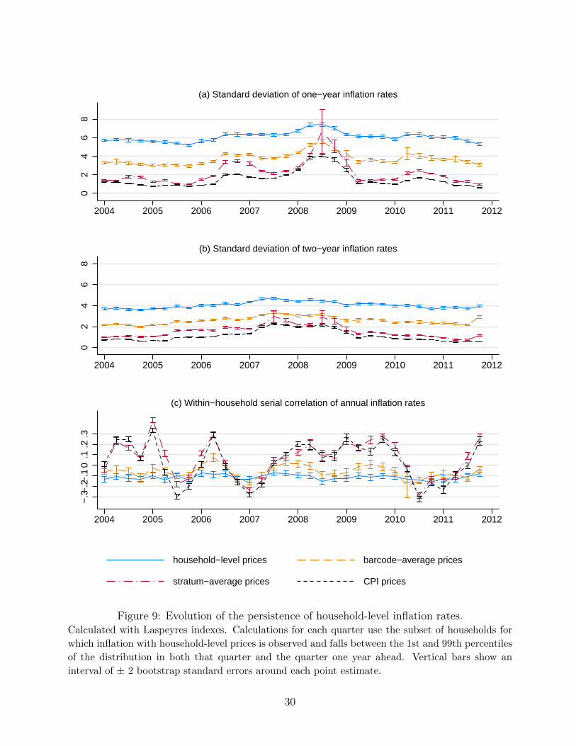
Figure 9 shows how the persistence of household-level inflation evolves over time. The
middle panel of the figure shows the cross-sectional standard deviation of annualized inflation
rates computed over two-year periods. The two-year inflation rates with household-level prices
remain highly dispersed, much more so than two-year inflation rates with stratum-average
or CPI prices, throughout the sample period. The standard deviation of two-year inflation
28

0.0
5.1
.15
dens
ity
−10 0 10 20household inflation rate (%)
(a) household prices0
.1.2
.3de
nsity
−10 0 10 20household inflation rate (%)
(b) barcode−average prices
0.2
5.5.
751
dens
ity
−10 0 10 20household inflation rate (%)
(c) stratum−average prices
0.2
5.5.
751
dens
ity
−10 0 10 20household inflation rate (%)
(d) CPI prices
2004−2005 2005−2006 2004−2006 annualized
Figure 8: Distributions of one-year and two-year household-level inflation rates, 2004q4–2005q4 and 2005q4–2006q4.Calculated with Laspeyres indexes. Kernel density estimates using Epanechnikov kernel. Bandwidth
is 0.05 percentage point for inflation rates with household-level and barcode-average prices and 0.005
percentage point for inflation rates with CPI prices. Sample limited to 19,252 households with
inflation rates calculated for both 2004q4–2005q4 and 2005q4–2006q4.
29
02
46
8
2004 2005 2006 2007 2008 2009 2010 2011 2012
(a) Standard deviation of one−year inflation rates0
24
68
2004 2005 2006 2007 2008 2009 2010 2011 2012
(b) Standard deviation of two−year inflation rates
−.3−
.2−.1
0.1
.2.3
2004 2005 2006 2007 2008 2009 2010 2011 2012
(c) Within−household serial correlation of annual inflation rates
household−level prices barcode−average prices
stratum−average prices CPI prices
Figure 9: Evolution of the persistence of household-level inflation rates.Calculated with Laspeyres indexes. Calculations for each quarter use the subset of households for
which inflation with household-level prices is observed and falls between the 1st and 99th percentiles
of the distribution in both that quarter and the quarter one year ahead. Vertical bars show an
interval of ± 2 bootstrap standard errors around each point estimate.
30

rates with barcode-average prices is about halfway between the results for CPI prices and
household-level prices, demonstrating that, as with one-year rates, variation in prices for a
given barcode and variation in the mix of barcodes within an item stratum are both important
sources of variation in household-level inflation rates. For comparison, the top panel of the
figure computes the cross-sectional standard deviation of one-year inflation rates among the
sample of households used to compute two-year rates (i.e., those with inflation rates observed
in consecutive years). The one-year rates are more dispersed than the two-year rates, showing
that heterogeneity in inflation rates does diminish when the inflation rate is computed over
a longer time horizon.
The bottom panel of Figure 9 computes the cross-sectional correlation between a
household’s inflation rate in quarter t and its inflation rate in quarter t + 4. The one-year
serial correlation of inflation rates using household-level prices is approximately −0.1, and
precisely estimated, throughout the sample period. This correlation is much less negative
than we would expect if households drew their price levels at random each period from the
cross-sectional distribution of price levels; in that case, the serial correlation would be −0.5.
Indeed, we can use the serial correlation of inflation rates to characterize a simple
stochastic process for household price levels. Assume that the deviation of a household’s
price level from the aggregate price level consists of a household fixed effect plus an AR(1)
process at an annual frequency. That is,
Pit − Pt = µi + ρ(Pi,t−4 − Pt−4 − µi) + εit, (14)
where Pit is the price level of household i in quarter t, Pt is the aggregate price level in quarter
t, µi is a household fixed effect, and εit is i.i.d. across households and over time with mean
zero and variance σ2. Also assume that households’ initial conditions are drawn from the
ergodic distribution, so that the distribution of Pit−Pt is stationary, which seems reasonable
given the relative stability of the standard deviations and serial correlations shown in Figure
9. Then
Var(πit) =2σ2
1 + ρ(15)
31
and
Cov(πit, πi,t−1) = σ2ρ− 1
1 + ρ, (16)
from which it follows that
ρ = 1 + 2Cov(πit, πi,t−1)
Var(πit)= 1 + 2Corr(πit, πi,t−1), (17)
where the second equality uses the stationarity of the distribution. Thus, a serial correlation of
inflation rates of −0.1 implies a serial correlation of price levels of ρ = 0.8. As a result, shocks
to households’ price levels are persistent but not permanent, according to this stochastic
process.
Together, the high cross-sectional variance and low serial correlation of household-level
inflation rates suggest that for individual households, the aggregate inflation rate is almost
irrelevant as a source of variation in the household-level inflation rate. Over the sample period,
our aggregate inflation rate averages 2.7 percent with a standard deviation of 1.9 percentage
points, whereas the cross-sectional standard deviation of household-level one-year inflation
rates averages 6.2 percentage points. If households’ deviations from aggregate inflation are
independent of the aggregate inflation rate, these figures mean that, over time, 91 percent
of the variance of a household’s annual inflation rate comes from heterogeneity — either the
household fixed effect µi or the idiosyncratic shocks εit — and only 9 percent from variability
in aggregate inflation.
5. Conclusion
This paper documents massive heterogeneity in inflation rates at the household level,
an order of magnitude larger than that found in previous work, owing to differences across
households in prices paid within the same categories of goods. Such heterogeneity poses a
range of challenges for monetary economics. Optimal policy in most monetary models is
calculated to maximize the welfare of a representative household that faces the aggregate
inflation rate; because extreme inflation rates cause larger welfare losses than small infla-
tion rates, optimal policy could be different if one accounted for heterogeneity in inflation
and for the policy’s effect on heterogeneity. In addition, even in models that relax the
32

representative-agent assumption by allowing uninsured shocks to generate heterogeneity in
assets and consumption, all households typically face the same inflation rate and hence the
same real interest rate (see, e.g., Kaplan, Moll, and Violante, 2015). Optimal policy might
differ if models allowed households to face identical nominal interest rates but, because in-
flation rates vary, different real rates. Furthermore, the heterogeneity we observe suggests
that movements of the aggregate price level may not be an important determinant of indi-
vidual agents’ inflation rates, potentially explaining why households and small firms fail to
be well informed about aggregate inflation and monetary policy (Binder, 2015; Kumar et al.,
forthcoming).
Heterogeneity in realized inflation could also help to explain heterogeneity in inflation
expectations. Allowing heterogeneity only in the allocation of spending across CPI item
strata, Johannsen (2014) shows that demographic groups with greater dispersion in realized
inflation also have greater dispersion in inflation expectations and proposes an imperfect
information model to explain this finding. Our results show that there is substantially more
heterogeneity in realized inflation once we account for differences in the allocation of spending
across goods within item strata and differences in prices paid for identical goods. The KNCP
does not measure inflation expectations, but it would be valuable for future researchers to
collect data on household-level inflation expectations and UPC-level purchasing patterns
within the same dataset so that the relationship between expectations and realized inflation
could be examined while allowing for all sources of heterogeneity.
However, the implications of household-level inflation heterogeneity depend impor-
tantly on whether households can forecast where they will fall in the cross-sectional distri-
bution. If a household has no idea where in the inflation distribution its particular inflation
rate will fall each year, the household’s best way to forecast its own inflation rate is still
to forecast the aggregate inflation rate. In such a case, while heterogeneity in realized in-
flation rates may have distributional consequences, it should have little impact on inflation
expectations or forward-looking decisions. By contrast, if households can predict whether
their own inflation rates will be above or below average, heterogeneity in inflation rates will
affect expectations and dynamic choices. Our data show that inflation rates at the household
level are only weakly correlated with observables and nearly serially uncorrelated. Thus, we
33

have little ability to forecast household-level deviations from aggregate inflation, either in the
cross-section or over time, with the limited information available to us as econometricians.
Whether households can use their much larger information sets to make better forecasts of
their idiosyncratic inflation rates is an important question that we leave for further research.
References
Angeletos, G. and Jennifer La’O, 2009, “Incomplete Information, Higher-Order Beliefs and
Price Inertia,” Journal of Monetary Economics 56, S19–S37.
Binder, Carola, 2015, “Fed Speak on Main Street,” manuscript, Haverford College.
Boskin, Michael J., Ellen R. Dulberger, Robert J. Gordon, Zvi Griliches, and Dale Jorgenson,
1996, “Toward a More Accurate Measure of the Cost of Living,” Final Report to the Senate
Finance Committee from the Advisory Commission to Study the Consumer Price Index,
accessed March 17, 2016, at https://www.ssa.gov/history/reports/boskinrpt.html.
Bronnenberg, Bart J., Jean-Pierre Dube, Matthew Gentzkow, and Jesse M. Shapiro, 2015,
“Do Pharmacists Buy Bayer? Informed Shoppers and the Brand Premium,” Quarterly
Journal of Economics 130(4), 1669–1726.
Bureau of Labor Statistics, 2015, “The Consumer Price Index,” in Handbook of Methods,
Washington: Bureau of Labor Statistics.
Einav, Liran, Ephraim Leibtag, and Aviv Nevo, 2010, “Recording Discrepancies in Nielsen
Homescan Data: Are They Present and Do They Matter?” Quantitative Marketing and
Economics 8(2), 207–239.
Federal Open Market Committee, 2016, “Statement on Longer-Run Goals and Monetary
Policy Strategy,” adopted effective Jan. 24, 2012, amended effective Jan. 26, 2016. Ac-
cessed March 22, 2016, at http://www.federalreserve.gov/monetarypolicy/files/
FOMC_LongerRunGoals_20160126.pdf.
Handbury, Jessie, 2013, “Are Poor Cities Cheap for Everyone? Non-homotheticity and the
Cost of Living Across U.S. Cities,” manuscript, University of Pennsylvania.
34
Hobijn, Bart, and David Lagakos, 2005, “Inflation Inequality in the United States,” Review
of Income and Wealth 51(4), 581–606.
Hobijn, Bart, Kristin Mayer, Carter Stennis, and Giorgio Topa, 2009, “Household Inflation
Experiences in the U.S.: A Comprehensive Approach,” Federal Reserve Bank of San Fran-
cisco Working Paper 2009-19.
Jaravel, Xavier, 2015, “The Unequal Gains from Product Innovations,” manuscript, Harvard
University.
Johannsen, Benjamin K., 2014, “Inflation Experience and Inflation Expectations: Dispersion
and Disagreement Within Demographic Groups,” Finance and Economics Discussion Series
2014-89, Board of Governors of the Federal Reserve System.
Kaplan, Greg, and Guido Menzio, 2015, “The Morphology of Price Dispersion,” International
Economic Review 56(4), 1165–1206.
Kaplan, Greg, Benjamin Moll, and Giovanni L. Violante, 2015, “Monetary Policy According
to HANK,” manuscript, Princeton University.
Kilts Center Archive of the Nielsen Company, 2013a, “Consumer Panel Dataset FAQ’s.”
Kilts Center Archive of the Nielsen Company, 2013b, “Consumer Panel Dataset Manual.”
Kumar, Saten, Hassan Afrouzi, Olivier Coibion, and Yuriy Gorodnichenko, forthcoming,
“Inflation Targeting Does Not Anchor Inflation Expectations: Evidence from Firms in
New Zealand,” Brookings Papers on Economic Activity.
Lucas, Robert E., Jr., 1972, “Expectations and the Neutrality of Money,” Journal of Eco-
nomic Theory 4(2), 103–124.
Lucas, Robert E., Jr., 1975, “An Equilibrium Model of the Business Cycle,” Journal of
Political Economy 83(6), 1113–1144.
Nimark, Kristoffer, 2008, “Dynamic Pricing and Imperfect Common Knowledge,” Journal of
Monetary Economics 55(2), 365–382.
35

Prais, S.J., 1959, “Whose Cost of Living?” Review of Economic Studies 26(2), 126–134.
Rao, J.N.K., C.F.J. Wu, and K. Yue, 1992, “Some Recent Work on Resampling Methods for
Complex Surveys,” Survey Methodology 18, 209–217.
Reis, Ricardo, 2006, “Inattentive Consumers,” Journal of Monetary Economics 53(8), 1761–
1800.
Sims, Christopher A., 2003, “Implications of Rational Inattention,” Journal of Monetary
Economics 50(3), 665–690.
36
Recommended