Hybrid Systems - Lecture n. 3Lyapunov stability
Maria Prandini
DEI - Politecnico di MilanoE-mail: [email protected]
OUTLINE
Focus: stability of equilibrium point
• continuous systems decribed by ordinary differentialequations (brief review)
• hybrid automata
OUTLINE
Focus: stability of equilibrium point
• continuous systems decribed by ordinary differentialequations (brief review)
• hybrid automata
ORDINARY DIFFERENTIAL EQUATIONS
An ordinary differential equation is a mathematical model of a continuous state continuous time system:
X = <n ≡ state spacef: <n → <n ≡ vector field (assigns a “velocity” vector to each x)

ORDINARY DIFFERENTIAL EQUATIONS
An ordinary differential equation is a mathematical model of a continuous state continuous time system:
X = <n ≡ state spacef: <n → <n ≡ vector field (assigns a “velocity” vector to each x)
Given an initial value x0 ∈ X,an execution (solution in the sense of Caratheodory) over the time interval [0,T) is a function x: [0,T) → <n such that:
• x(0) = x0
• x is continuous and piecewise differentiable
•
ODE SOLUTION: WELL-POSEDNESS
Theorem [local existence non-blocking]If f: <n → <n is continuous, then ∀x0 there exists at least a solution with x(0)=x0 defined on some [0,δ).
Theorem [local existence and uniqueness non-blocking, deterministic]If f: <n → <n is Lipschitz continuous, then ∀ x0 there exists a single solution with x(0)=x0 defined on some [0,δ).
Theorem [global existence and uniqueness non-blocking, deterministic, non-Zeno]If f: <n → <n is globally Lipschitz continuous, then ∀ x0 thereexists a single solution with x(0)=x0 defined on [0,∞).
STABILITY OF CONTINUOUS SYSTEMS
with f: <n → <n globally Lipschitz continuous
Definition (equilibrium): xe ∈ <n for which f(xe)=0
Remark: xe is an invariant set
Definition (stable equilibrium):The equilibrium point xe ∈ <n is stable (in the sense ofLyapunov) if
execution startingfrom x(0)=x0
Definition (stable equilibrium):
Graphically:
δxe
equilibrium motion
perturbed motion
ε
small perturbations lead to small changes in behavior

Definition (stable equilibrium):
Graphically:
small perturbations lead to small changes in behavior
δxe
ε phase plot
Definition (asymptotically stable equilibrium):
and δ can be chosen so that
Graphically:
δxe
equilibrium motion
perturbed motion
ε
small perturbations lead to small changes in behaviorand are re-absorbed, in the long run
Definition (asymptotically stable equilibrium):
and δ can be chosen so that
Graphically:
small perturbations lead to small changes in behaviorand are re-absorbed, in the long run
δxe
ε
EXAMPLE: PENDULUM
m
l
frictioncoefficient (α)
EXAMPLE: PENDULUM
unstable equilibrium
m EXAMPLE: PENDULUM
as. stable equilibriumm
EXAMPLE: PENDULUM
m
l
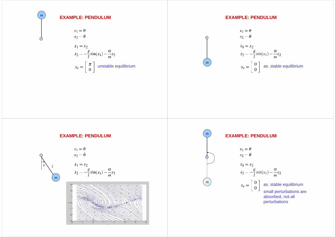
EXAMPLE: PENDULUM
as. stable equilibrium
small perturbations are absorbed, not allperturbations
m
m

Let xe be asymptotically stable.
Definition (domain of attraction):The domain of attraction of xe is the set of x0 such that
Definition (globally asymptotically stable equilibrium):xe is globally asymptotically stable (GAS) if its domain ofattraction is the whole state space <n
More definitions: exponentially stable, globally exponentially stable, ...
execution startingfrom x(0)=x0
STABILITY OF CONTINUOUS SYSTEMS
with f: <n → <n globally Lipschitz continuous
Definition (equilibrium): xe ∈ <n for which f(xe)=0
Without loss of generality we suppose that
xe = 0if not, then z := x -xe → dz/dt = g(z), g(z) := f(z+xe) (g(0) = 0)
STABILITY OF CONTINUOUS SYSTEMS
with f: <n → <n globally Lipschitz continuous
How to prove stability?find a function V: <n → < such that
V(0) = 0 and V(x) >0, for all x ≠ 0V(x) is decreasing along the executions of the system
V(x) = 3
V(x) = 2
x(t)
STABILITY OF CONTINUOUS SYSTEMS
execution x(t)
candidate function V(x)
behavior of V along the execution x(t): V(t): = V(x(t))
Advantage with respect to exhaustive check of all executions?

with f: <n → <n globally Lipschitz continuous
V: <n → < continuously differentiable (C1) function
Rate of change of V along the execution of the ODE system:
STABILITY OF CONTINUOUS SYSTEMS
gradient vector
No need to solve the ODE for evaluating if V(x) decreasesalong the executions of the system
LYAPUNOV STABILITY
Theorem (Lyapunov stability Theorem):Let xe = 0 be an equilibrium for the system and D⊂ <n an open
set containing xe = 0. If V: D → < is a C1 function such that
Then, xe is stable.
V positive definite on D
V non increasing alongsystem executions in D(negative semidefinite)
LYAPUNOV STABILITY
Theorem (Lyapunov stability Theorem):Let xe = 0 be an equilibrium for the system and D⊂ <n an open
set containing xe = 0. If V: D → < is a C1 function such that
Then, xe is stable.
Lyapunov functionfor the system and the equilibrium xe
Finding Lyapunov functions is HARD in generalSufficient condition
Proof:
Given ε >0, choose r∈ (0,ε) such that Br = x∈ <n: ||x|| · r ⊂ DSet α : = minV(x): ||x|| = r > 0 and choose c ∈ (0,α). Then,
Ωc := x: V(x) · c ⊂ Br
Since then V(x(t))· V(x(0)), ∀ t≥ 0. Hence, all executions starting in Ωc stays in Ωc.
V(x) is continuous and V(0) = 0. Then, there is δ >0 such that Bδ = x∈ <n: ||x|| · δ ⊂ Ωc .
Therefore, ∀ ||x(0)|| < δ ⇒ ||x(t)|| < ε, ∀ t≥ 0

EXAMPLE: PENDULUM
m
l
frictioncoefficient (α)
energy function
xe stable
LYAPUNOV STABILITY
Theorem (Lyapunov stability Theorem):Let xe = 0 be an equilibrium for the system and D⊂ <n an open
set containing xe = 0. If V: D → < is a C1 function such that
Then, xe is stable.
If it holds also that
Then, xe is asymptotically stable (AS)
LYAPUNOV GAS THEOREM
Theorem (Barbashin-Krasovski Theorem):Let xe = 0 be an equilibrium for the system.
If V: <n → < is a C1 function such that
Then, xe is globally asymptotically stable (GAS).
V positive definite on <n
V decreasing alongsystem executions in <n
(negative definite)
V radially unbounded
STABILITY OF LINEAR CONTINUOUS SYSTEMS
• xe = 0 is an equilibrium for the system
• the elements of matrix eAt are linear combinations of eλi(A)t, i=1,2,…,n

STABILITY OF LINEAR CONTINUOUS SYSTEMS
• xe = 0 is an equilibrium for the system
• xe =0 is asymptotically stable if and only if A is Hurwitz (all eigenvalues with real part <0)
• asymptotic stability ≡ GAS
STABILITY OF LINEAR CONTINUOUS SYSTEMS
• xe = 0 is an equilibrium for the system
• xe =0 is asymptotically stable if and only if A is Hurwitz (alleigenvalues with real part <0)
• asymptotic stability ≡ GAS
Alternative characterization…
STABILITY OF LINEAR CONTINUOUS SYSTEMS
Theorem (necessary and sufficient condition):
The equilibrium point xe =0 is asymptotically stable if and onlyif for all matrices Q = QT positive definite (Q>0) the
ATP+PA = -Q
has a unique solution P=PT >0.
Lyapunov equation
STABILITY OF LINEAR CONTINUOUS SYSTEMS
Theorem (necessary and sufficient condition):
The equilibrium point xe =0 is asymptotically stable if and onlyif for all matrices Q = QT positive definite (Q>0) the
ATP+PA = -Q
has a unique solution P=PT >0.
Remarks: Q positive definite (Q>0) iff xTQx >0 for all x ≠ 0Q positive semidefinite (Q≥ 0) iff xTQx ≥ 0 for all x and xT Q x = 0 for some x ≠ 0
Lyapunov equation

STABILITY OF LINEAR CONTINUOUS SYSTEMS
Theorem (necessary and sufficient condition):
The equilibrium point xe =0 is asymptotically stable if and onlyif for all matrices Q = QT positive definite (Q>0) the
ATP+PA = -Q
has a unique solution P=PT >0.
Proof.
(if) V(x) =xT P x is a Lyapunov function
Lyapunov equation
STABILITY OF LINEAR CONTINUOUS SYSTEMS
Theorem (necessary and sufficient condition):
The equilibrium point xe =0 is asymptotically stable if and onlyif for all matrices Q = QT positive definite (Q>0) the
ATP+PA = -Q
has a unique solution P=PT >0.
Proof.
(only if) Consider
Lyapunov equation
STABILITY OF LINEAR CONTINUOUS SYSTEMS
Theorem (necessary and sufficient condition):
The equilibrium point xe =0 is asymptotically stable if and onlyif for all matrices Q = QT positive definite (Q>0) the
ATP+PA = -Q
has a unique solution P=PT >0.
Proof.
(only if) Consider
P = PT and P>0 easy to show
P unique by contradiction
Lyapunov equation
STABILITY OF LINEAR CONTINUOUS SYSTEMS
Theorem (necessary and sufficient condition):
The equilibrium point xe =0 is asymptotically stable if and onlyif for all matrices Q = QT positive definite (Q>0) the
ATP+PA = -Q
has a unique solution P=PT >0.
Remarks: for a linear system
• existence of a (quadratic) Lyapunov function V(x) =xT P x is a necessary and sufficient condition
• it is easy to compute a Lyapunov function since the Lyapunovequation is a linear algebraic equation
Lyapunov equation
STABILITY OF LINEAR CONTINUOUS SYSTEMS
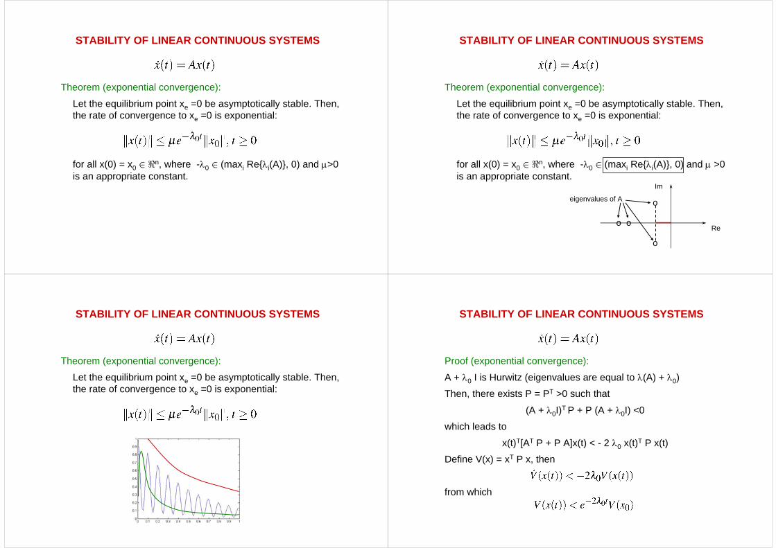
Theorem (exponential convergence):
Let the equilibrium point xe =0 be asymptotically stable. Then, the rate of convergence to xe =0 is exponential:
for all x(0) = x0 ∈ <n, where -λ0 ∈ (maxi Reλi(A), 0) and µ>0 is an appropriate constant.
STABILITY OF LINEAR CONTINUOUS SYSTEMS
Theorem (exponential convergence):
Let the equilibrium point xe =0 be asymptotically stable. Then, the rate of convergence to xe =0 is exponential:
for all x(0) = x0 ∈ <n, where -λ0 ∈ (maxi Reλi(A), 0) and µ >0 is an appropriate constant.
Re
Im
o
o
o o
eigenvalues of A
STABILITY OF LINEAR CONTINUOUS SYSTEMS
Theorem (exponential convergence):
Let the equilibrium point xe =0 be asymptotically stable. Then, the rate of convergence to xe =0 is exponential:
STABILITY OF LINEAR CONTINUOUS SYSTEMS
Proof (exponential convergence):
A + λ0 I is Hurwitz (eigenvalues are equal to λ(A) + λ0)
Then, there exists P = PT >0 such that
(A + λ0I)T P + P (A + λ0I) <0which leads to
x(t)T[AT P + P A]x(t) < - 2 λ0 x(t)T P x(t) Define V(x) = xT P x, then
from which

STABILITY OF LINEAR CONTINUOUS SYSTEMS
(cont’d) Proof (exponential convergence):
thus finally leading to
STABILITY OF LINEAR CONTINUOUS SYSTEMS
(cont’d) Proof (exponential convergence):
thus finally leading to
OUTLINE
Focus: stability of equilibrium point
• continuous systems decribed by ordinary differentialequations (brief review)
• hybrid automata
HYBRID AUTOMATA: FORMAL DEFINITION
A hybrid automaton H is a collection
H = (Q,X,f,Init,Dom,E,G,R)• Q = q1,q2, … is a set of discrete states (modes)
• X = <n is the continuous state space
• f: Q× X→ <n is a set of vector fields on X
• Init ⊆ Q× X is a set of initial states
• Dom: Q → 2X assigns to each q∈ Q a domain Dom(q) of X
• E ⊆ Q× Q is a set of transitions (edges)
• G: E → 2X is a set of guards (guard condition)
• R: E× X → 2X is a set of reset maps

q = q1
q = q2
HYBRID TIME SET
A hybrid time set is a finite or infinite sequence of intervals
τ = Ii, i=0,1,…, M such that
• Ii = [τi, τi’] for i < M • IM = [τM, τM’] or IM = [τM, τM’) if M<∞
• τi’ = τi+1
• τi · τi’
[ ][ ]
[ ]
τ0
I0
τ0’
τ1 τ1’I1
I2 τ2 = τ2’
τ3 τ3’I3
HYBRID TIME SET
A hybrid time set is a finite or infinite sequence of intervals
τ = Ii, i=0,1,…, M such that
• Ii = [τi, τi’] for i < M • IM = [τM, τM’] or IM = [τM, τM’) if M<∞
• τi’ = τi+1
• τi · τi’
[ ][ ]
[ ]
τ0
I0
τ0’
τ1 τ1’I1
I2 τ2 = τ2’
τ3 τ3’I3
t1
t2
t3
t4
t1 ≺ t2 ≺ t3 ≺ t4
the elements of τ arelinearly ordered
τ∞ := ∑i(τi’-τi)(continuous extent)
HYBRID TRAJECTORY
A hybrid trajectory (τ, q, x) consists of:
• A hybrid time set τ = Ii, i=0,1,…, M • Two sequences of functions q = qi(·), i=0,1,…, M and x =
xi(·), i=0,1,…, M such that
qi: Ii → Q
xi: Ii → X

HYBRID AUTOMATA: EXECUTION
A hybrid trajectory (τ, q, x) is an execution (solution) of the hybrid automaton H = (Q,X,f,Init,Dom,E,G,R) if it satisfies the following conditions:
• Initial condition: (q0(τ0), x0(τ0)) ∈ Init
• Continuous evolution:for all i such that τi < τi’
qi: Ii → Q is constantxi:Ii→ X is the solution to the ODE associated with qi(τi)xi(t) ∈ Dom(qi(τi)), t∈ [τi,τi’)
• Discrete evolution:(qi(τi’),qi+1(τi+1)) ∈ E transition is feasiblexi(τi’) ∈ G((qi(τi’),qi+1(τi+1))) guard condition satisfiedxi(τi+1) ∈ R((qi(τi’),qi+1(τi+1)),xi(τi’)) reset condition satisfied
HYBRID AUTOMATA: EXECUTION
Well-posedness?
Problems due the hybrid nature:
for some initial state (q,x)• infinite execution of finite duration Zeno • no infinite execution blocking • multiple executions non-deterministic
We denote by
H(q,x) the set of (maximal) executions of H starting from (q,x)
H(q,x)∞ the set of infinite executions of H starting from (q,x)
STABILITY OF HYBRID AUTOMATA
H = (Q,X,f,Init,Dom,E,G,R)
Definition (equilibrium): xe =0 ∈ X is an equilibrium point of H if:• f(q,0) = 0 for all q ∈ Q• ((q,q’)∈ E) ∧ (0∈ G((q,q’)) ⇒ R((q,q’),0) = 0
Remarks:
• discrete transitions are allowed out of (q,0) but only to (q’,0)• for all (q,0) ∈ Init and (τ, q, x) is an execution of H starting
from (q,0), then x(t) = 0 for all t∈ τ
EXAMPLE: SWITCHING LINEAR SYSTEM
H = (Q,X,f,Init,Dom,E,G,R)
• Q = q1, q2 X = <2
• f(q1,x) = A1x and f(q2,x) = A2x with:
• Init = Q × x∈ X: ||x|| >0
• Dom(q1) = x∈ X: x1x2 · 0 Dom(q2) = x∈ X: x1x2 ≥ 0
• E = (q1,q2),(q2,q1)• G((q1,q2)) = x∈ X: x1x2 ≥ 0 G((q2,q1)) = x∈ X: x1x2 · 0
• R((q1,q2),x) = R((q2,q1),x) = x
xe = 0 is an equilibrium: f(q,0) = 0 & R((q,q’),0) = 0

H = (Q,X,f,Init,Dom,E,G,R)
Definition (stable equilibrium): Let xe = 0 ∈ X be an equilibrium point of H. xe = 0 is stable if
Remark:
• Stability does not imply convergence
• To analyse convergence, only infinite executions should beconsidered
STABILITY OF HYBRID AUTOMATA
set of (maximal) executionsstarting from (q0, x0) ∈ Init
H = (Q,X,f,Init,Dom,E,G,R)
Definition (stable equilibrium): Let xe = 0 ∈ X be an equilibrium point of H. xe = 0 is stable if
Definition (asymptotically stable equilibrium): Let xe = 0 ∈ X be an equilibrium point of H. xe = 0 is asymptotically
stable if δ>0 that can be chosen so that
STABILITY OF HYBRID AUTOMATA
set of (maximal) executionsstarting from (q0, x0) ∈ Init
set of infinite executionsstarting from (q0, x0) ∈ Initτ∞ < ∞ if Zeno
H = (Q,X,f,Init,Dom,E,G,R)
Definition (stable equilibrium): Let xe = 0 ∈ X be an equilibrium point of H. xe = 0 is stable if
Question:
xe = 0 stable equilibrium for each continuous system dx/dt = f(q,x) implies that xe = 0 stable equilibrium for H?
STABILITY OF HYBRID AUTOMATA EXAMPLE: SWITCHING LINEAR SYSTEM
H = (Q,X,f,Init,Dom,E,G,R)
• Q = q1, q2 X = <2
• f(q1,x) = A1x and f(q2,x) = A2x with:
• Init = Q × x∈ X: ||x|| >0
• Dom(q1) = x∈ X: x1x2 · 0 Dom(q2) = x∈ X: x1x2 ≥ 0
• E = (q1,q2),(q2,q1)• G((q1,q2)) = x∈ X: x1x2 ≥ 0 G((q2,q1)) = x∈ X: x1x2 · 0
• R((q1,q2),x) = R((q2,q1),x) = x
xe = 0 is an equilibrium: f(q,0) = 0 & R((q,q’),0) = 0

EXAMPLE: SWITCHING LINEAR SYSTEM
Asymptotically stable linear systems.
EXAMPLE: SWITCHING LINEAR SYSTEM
q1: quadrants 2 and 4q2: quadrants 1 and 3
Asymptotically stable linear systems, but xe = 0 unstableequilibrium of H
EXAMPLE: SWITCHING LINEAR SYSTEM
q1: quadrants 1 and 3q2: quadrants 2 and 4
EXAMPLE: SWITCHING LINEAR SYSTEM
||x(τi)|| < ||x(τi+1)|| ||x(τi)|| > ||x(τi+1)||overshoots sum up

LYAPUNOV STABILITY
H = (Q,X,f,Init,Dom,E,G,R)
Theorem (Lyapunov stability):Let xe = 0 be an equilibrium for H with R((q,q’),x) = x, ∀ (q,q’)∈ E, and
D⊂ X=<n an open set containing xe = 0. Consider V: Q× D → < is a C1 function in x such that for all q ∈ Q:
If for all (τ, q, x) ∈ H(q0,x0) with (q0,x0) ∈ Init ∩ (Q× D), and all q’∈ Q, the sequence V(q(τi),x(τi)): q(τi) =q’ is non-increasing (or empty),
then, xe = 0 is a stable equilibrium of H.
V(q,x) Lyapunov functionfor continuous system q⇒ xe =0 is stableequilibrium for system q
LYAPUNOV STABILITY
H = (Q,X,f,Init,Dom,E,G,R)
Sketch of the proof.
V(q(t),x(t))V(q1,x(t))
[ ][ ][ ][ q(t)= q1 q(t)= q1V(q2,x(t))
τ0 τ0’=τ1 τ1’=τ2 τ2’=τ3
Lyapunov function forsystem q1 → decreaseswhen q(t) = q1, but can increase when q(t) ≠ q1
LYAPUNOV STABILITY
H = (Q,X,f,Init,Dom,E,G,R)
Sketch of the proof.
V(q(t),x(t))V(q1,x(t))
[ ]τ0 τ0’=τ1
[ ][ ]τ1’=τ2 τ2’=τ3
[ q(t)= q1 q(t)= q1
V(q1,x(τi))non-increasing

LYAPUNOV STABILITY
H = (Q,X,f,Init,Dom,E,G,R)
Sketch of the proof.
V(q(t),x(t))V(q1,x(t))
[ ]τ0 τ0’=τ1
[ ][ ]τ1’=τ2 τ2’=τ3
[ q(t)= q1 q(t)= q1
LYAPUNOV STABILITY
H = (Q,X,f,Init,Dom,E,G,R)
V(q(t),x(t)) Lyapunov-like function
EXAMPLE: SWITCHING LINEAR SYSTEM
H = (Q,X,f,Init,Dom,E,G,R)
• Q = q1, q2 X = <2
• f(q1,x) = A1x and f(q2,x) = A2x with:
• Init = Q × x∈ X: ||x|| >0
• Dom(q1) = x∈ X: Cx ≥ 0 Dom(q2) = x∈ X: Cx · 0
• E = (q1,q2),(q2,q1)• G((q1,q2)) = x∈ X: Cx · 0 G((q2,q1)) = x∈ X: Cx ≥ 0, CT∈ <2
• R((q1,q2),x) = R((q2,q1),x) = x
EXAMPLE: SWITCHING LINEAR SYSTEM
H = (Q,X,f,Init,Dom,E,G,R)
q1q2

EXAMPLE: SWITCHING LINEAR SYSTEM
Proof that xe = 0 is a stable equilibrium of H for any CT∈ <2 :
• xe = 0 is an equilibrium: f(q1,0) = f(q2,0) = 0
R((q1,q2),0) = R((q2,q1),0) = 0
• xe = 0 is stable:
consider the candidate Lyapunov-like function:
V(qi,x) = xT Pi x,
where Pi =PiT >0 solution to Ai
T Pi + Pi Ai = - I
(V(qi,x) is a Lyapunov function for the asymptotically stablelinear system qi)
In each discrete state, the continuous system is as. stable...
EXAMPLE: SWITCHING LINEAR SYSTEM
Proof that xe = 0 is a stable equilibrium of H for any CT∈ <2:
• xe = 0 is an equilibrium: f(q1,0) = f(q2,0) = 0
R((q1,q2),0) = R((q2,q1),0) = 0
• xe = 0 is stable:
consider the candidate Lyapunov-like function:
V(qi,x) = xT Pi x,
where Pi =PiT >0 solution to Ai
T Pi + Pi Ai = - I
EXAMPLE: SWITCHING LINEAR SYSTEM
Test for non-increasing sequence condition
The level sets of V(qi,x) = xTPi x are ellipses centered at the origin. A level set intersects the switching line CTx =0 at z and -z.
CTx = 0
z
-z
τi
τi’=τi+1
τi+2
EXAMPLE: SWITCHING LINEAR SYSTEM
Test for non-increasing sequence condition
The level sets of V(qi,x) = xTPi x are ellipses centered at the origin. A level set intersects the switching line CTx =0 at z and -z.
Let q(τi)=q1 and x(τi)=z.
Since V(q1,x(t)) is not increasing during [τi,τi’], then, when x(t) intersects the switching line at τi’, it does at α z with α ∈ (0,1], hence ||x(τi+1)|| = ||x(τi’)|| · ||x(τi)||. Let q(τi+1)=q2
Since V(q2,x(t)) is decreasing during [τi+1,τi+1’], then, when x(t) intersects the switching line at τi+1’, ||x(τi+2)|| = ||x(τi+1’)|| · ||x(τi+1)|| · ||x(τi)||
From this, it follows that V(q1,x(τi+2)) · V(q1,x(τi))

LYAPUNOV STABILITY
H = (Q,X,f,Init,Dom,E,G,R)
Drawbacks:
• The sequence V(q(τi),x(τi)): q(τi) =q’ must be evaluated, whichmay require solving the ODEs
• In general, it is hard to find a Lyapunov-like function
LYAPUNOV STABILITY
H = (Q,X,f,Init,Dom,E,G,R)
Corollary (Lyapunov stability Theorem):Let xe = 0 be an equilibrium for H with R((q,q’),x) = x, ∀
(q,q’)∈ E, and D⊂ X=<n an open set containing xe = 0.
If V: D → < is a C1 function such that for all q ∈ Q:
then, xe = 0 is a stable equilibrium of H.
Proof: Define W(q,x) = V(x), ∀ q ∈ Q and apply the theorem
V(x) common Lyapunovfunction for all systems q
t
))(( txVsame V function+ identity reset map
COMPUTATIONAL LYAPUNOV METHODS
HPL = (Q,X,f,Init,Dom,E,G,R)
non-Zeno and such that for all qk∈ Q:• f(qk,x) = Ak x
(linear vector fields)• Init ⊂ ∪q∈ Q q × Dom(q)
(admissible initialization)• for all x∈ X, the set
Jump(qk,x):= (q’,x’): (qk,q’)∈ E, x∈G((qk,q’)), x’∈R((q,q’),x)has cardinality 1 if x ∈ ∂Dom(q), 0 otherwise(discrete transitions occur only from the boundary of the domains)
• (q’,x’) ∈ Jump(qk,x) → x’∈ Dom(q’) and x’ = x(trivial reset for x)
For this class of Piecewise Linear hybrid automata computationallyattractive methods exist to construct the Lyapunov-like function

GLOBALLY QUADRATIC LYAPUNOV FUNCTION
HPL = (Q,X,f,Init,Dom,E,G,R)
Theorem (globally quadratic Lyapunov function):
Let xe = 0 be an equilibrium for HPL.
If there exists P=PT >0 such thatAk
T P+ PAk < 0, ∀ k
Then, xe = 0 is asymptotically stable.
Proof.
V(x) = xT Px is a common Lyapunov function
GLOBALLY QUADRATIC LYAPUNOV FUNCTION
Alternative proof (showing exponential convergence):There exists γ >0 such that Ak
T P+ PAk +γ I · 0, ∀ k
There exists a unique, infinite, non-Zeno execution (τ,q,x) forevery initial state with x: τ → <n satisfying
where µk: τ → [0,1] is such that ∑k µk(t)=1, t∈ [τi,τi’].
Let V(x) = xT Px. Then, for t∈ [τi,τi’).
GLOBALLY QUADRATIC LYAPUNOV FUNCTION
Sketch of the proof. (cont’d)Since λmin(P) ||x||2 · V(x) · λmax(P) ||x||2, then
and, hence,
which leads to
Then,
Since τ∞ =∞ (non-Zeno), then ||x(t)|| goes to zero exponentially as t→ τ∞
GLOBALLY QUADRATIC LYAPUNOV FUNCTION
q1q2
conditions of the theoremsatisfied with P = I

GLOBALLY QUADRATIC LYAPUNOV FUNCTION
HPL = (Q,X,f,Init,Dom,E,G,R)
Theorem (globally quadratic Lyapunov function):
Let xe = 0 be an equilibrium for HPL.
If there exists P=PT >0 such thatAk
T P+ PAk < 0, ∀ k
Then, xe = 0 is asymptotically stable.
Remark:
A set of LMIs to solve. This problem can be reformulated as a convex optimization problem. Efficient solvers exist.
GLOBALLY QUADRATIC LYAPUNOV FUNCTION
• A globally quadratic Lyapunov function does not exist if and only if there exist positive definite symmetric matrices Rksuch that
GLOBALLY QUADRATIC LYAPUNOV FUNCTION
q1q2
conditions of the theoremNOT satisfied for any P but xe = 0 stable equilibrium
stable node stable focus
piecewise quadraticLyapunov function
PIECWISE QUADRATIC LYAPUNOV FUNCTION
• Developed for piecewise linear systems with structureddomain (set of convex polyhedra) and reset
• Resulting Lyapunov function is continuous at the switchingtimes
• LMIs characterization

REFERENCES
• H.K. Khalil. Nonlinear Systems.Prentice Hall, 1996.
• S. Boyd, L. El Ghaoui, E. Feron, and V. Balakrishnan.Linear Matrix Inequalities in System and Control Theory.SIAM, 1994.
• M. Branicky. Multiple Lyapunov functions and other analysis tools for switched and hybrid systems.IEEE Trans. on Automatic Control, 43(4):475-482, 1998.
• H. Ye, A. Michel, and L. Hou. Stability theory for hybrid dynamical systems. IEEE Transactions on Automatic Control, 43(4):461-474, 1998.
• M. Johansson and A. Rantzer.Computation of piecewise quadratic Lyapunov function for hybridsystems. IEEE Transactions on Automatic Control, 43(4):555-559, 1998.
• R.A. Decarlo, M.S. Branicky, S. Petterson, and B. Lennartson.Perspectives and results on the stability and stabilization of hybridsystems. Proceedings of the IEEE, 88(7):1069-1082, 2000.
Recommended