
HUMAN ACTIVITY RECOGNITION USING BODY
AREA SENSOR NETWORKS
By
BO XU
Bachelor of Science in Electronic Engineering
University of Science and Technology Beijing
Beijing, China
2005
Submitted to the Faculty of the Graduate College of the Oklahoma State University in partial fulfillment of the requirements for the Degree of MASTER OF SCIENCE
May, 2009

ii
HUMAN ACTIVITY RECOGNITION USING BODY
AREA SENSOR NETWORKS
Thesis Approved: Xiaolin Li
Thesis Adviser Weihua Sheng Venkatesh Sarangan
A. Gordon Emslie
Dean of the Graduate College

iii
ACKNOWLEDGMENTS
I would like to express my gratitude to my supervisor, Dr. Xiaolin Li, whose
expertise, understanding, and patience, added considerably to my graduate experience. I
appreciate his vast knowledge and skill in many areas, and his assistance in writing this
thesis. I would also like to thank other members of my committee, Dr. Weihua Sheng,
and Dr. Venkatesh Sarangan for the assistance they provided at all levels of the research
project. Finally, I would like to thank my parents to support me go to United States,
where I learned a lot both in my study and in my life.

iv
TABLE OF CONTENTS Chapter Page 1. INTRODUCTION .....................................................................................................1
1.1 Wireless Sensor Networks .................................................................................1 1.2 Wireless Body Area Networks...........................................................................2 1.3 Hidden Markov Model .......................................................................................3 2. REVIEW OF LITERATURE AND SYSTEM ARCHITECTURE ..........................5 2.1 The Application of Hidden Markov Model .......................................................5 2.2 System Architecture for HMM Based Human Activities Identification ...........6 3. METHODOLOGY OF HUMAN ACTIVITIES RECOGNITION ...........................7 3.1 Data Collection ..................................................................................................7 3.1.1 Hardware Selection ...................................................................................7 3.2 TinyOS ...............................................................................................................9 3.3 Data Collection ..................................................................................................9
3.3.1 Sensor Nodes Data Collection ..................................................................9 3.3.2 Wireless Pulse Oximeter Data Collection ...............................................12 3.4 Data Parsing .....................................................................................................12 3.4.1 Observation Sequence Classification ......................................................13 3.4.2 Hidden States Definition .........................................................................16 3.5 Hidden Markov Model Training using Baum-Welch Algorithm ....................17
3.5.1 Baum-Welch Algorithm ..........................................................................18 3.6 Hidden States Decoding ...................................................................................20 4. EXTENDED KALMAN FILTER IN INDOOR LOCALIZATION .......................22
4.1 Kalman Filter ...................................................................................................22 4.2 Extended Kalman Filter ...................................................................................25 4.3 Application of Extended Kalman Filter in Indoor Localization ......................26
4.3.1 RSSI Based Distance measurement ........................................................26 4.3.2 System Model .........................................................................................28

v
Chapter Page
5. CONCLUSION AND FUTURE WORK ................................................................32 5.1 Human Activities Recognition Result… .........................................................32 5.2 Indoor Localization Result………………………………………………….. 40
5.2.1 Experiment Set-up ..................................................................................40 5.2.2 Experiment Result ...................................................................................42
5.3 Conclusion and Future Work ...........................................................................51 REFERENCES ............................................................................................................53

vi
LIST OF TABLES Table Page Table 2.1 PC/Laptop Side Architecture ........................................................................ 6 Table 2.2 Motes Side Architecture ................................................................................6
vii
LIST OF FIGURES Figure Page Figure 3.1 Sensor nodes distributed in one subject ....................................................10 Figure 3.2 Crossbow Micaz sensor node and MTS400 sensor board ........................11 Figure 3.3 Data Collection Mechanism .....................................................................12 Figure 3.4 Four Parts of Wireless Pulse Oximeter ....................................................12 Figure 3.5 Component Structure in Wireless Pulse Oximeter ...................................13 Figure 3.6 Observation Sequence Classification .......................................................15 Figure 3.7 States Transition Form for Hidden States ................................................17 Figure 4.1 Relation between distance and RSSI ........................................................28 Figure 5.1 Reluctant Acceleration Data for Proposition 1 .........................................32 Figure 5.2 Hidden States Decoding for Proposition 1 ...............................................33 Figure 5.3 Reluctant Acceleration Data for Proposition 2 .........................................34 Figure 5.4 Hidden States Decoding for Proposition 2 ...............................................34 Figure 5.5 Reluctant Acceleration Data for Proposition 3 .........................................36 Figure 5.6 Hidden States Decoding for Proposition 3 ...............................................36 Figure 5.7 Accuracy of human activities recognition with HMM and without
HMM........................................................................................................37 Figure 5.8 Subject using his/her own model and Subject using other trainee’s
model........................................................................................................38 Figure 5.9 Comparison of accuracy for human activities with one sensor, two
sensors and three sensors mounted on each subject ................................39 Figure 5.10 Comparison of accuracy among sensors mounted on different parts of
human body ............................................................................................40 Figure 5.11 Two target nodes deployed vertically to record three axis
acceleration data .....................................................................................42 Figure 5.12 Real route coordinate, EKF implemented coordinate, in a
1.8m*2.1m*1.5m area (walk diagonally) ..............................................42 Figure 5.13 X-axis data for EKF coordinate, real route coordinate ...........................43 Figure 5.14 Y-axis data for EKF coordinate, real route coordinate ...........................43 Figure 5.15 Z-axis data for EKF coordinate, real route coordinate ...........................44 Figure 5.16 Average error for EKF in three axis in the 1.8m*2.1m*1.5m area ........44 Figure 5.17 Real route coordinate, EKF implemented coordinate, calculated
coordinate in a 1.8m*2.1m*1.5m area (walk straightly) .......................45 Figure 5.18 X-axis coordinate of EKF and real route ................................................46 Figure 5.19 Y-axis coordinate of EKF and real route ................................................46 Figure 5.20 Z-axis coordinate of EKF and real route ................................................46 Figure 5.21 Average error for EKF in three axis in the 1.8m*2.1m*1.5m

viii
Figure Page
area .........................................................................................................47 Figure 5.22 Real route coordinate, EKF implemented coordinate, in a
1.8m*6m*1.5m area (walk diagonally) .................................................48 Figure 5.23 X-axis coordinate of EKF and real route ................................................49 Figure 5.24 Y-axis coordinate of EKF and real route ................................................49 Figure 5.25 Z-axis coordinate of EKF and real route ................................................49 Figure 5.26 Average error for EKF in three axis in the 1.8m*6m*1.5m
area (walk diagonally) .............................................................................50

1
CHAPTER 1
INTRODUCTION
1.1 Wireless Sensor Networks
As an emerging technology that bridges the physical world and the digital
information world, wireless sensor networks provide a tiny, low-power and low cost but
powerful platforms for data collection and transmission [1]. A wireless sensor network
consists of distributed smart devices equipped with processor, radio, memory, and
sensors, monitoring physical or environmental conditions cooperatively in multiple
modalities, for example, temperature, humidity, sound, motion, vibration and so on.
Wireless sensor networks are now used in many areas, such as traffic control, precision
agriculture, environment and habitat monitoring, healthcare applications, home
automation, and so on.
Wireless sensor networks consist of many sensor nodes which can be considered as
miniature computers. Each sensor node is equipped with a microcontroller, a radio
transceiver or other communications device, and an energy supply, usually a battery.
This thesis will focus on human activity recognition using wireless sensor networks.
Each human being will be equipped with several sensor nodes in his/her body to build up
a body area sensor network. Sensor data will be saved and later processed for training and
analysis purpose. The other topic investigated in this thesis is indoor localization. Our
method uses RSSI based distance measurement and Extended Kalman Filter. The

2
distance measured is used as input data in the Extended Kalman Filter to get the location
of a target node. In the next section, we will briefly introduce body area sensor networks.
1.2 Wireless Body Area Sensor Networks
Wireless body area sensor networks (WBASNs) are an extension of wireless sensor
network,which focus on the application of wireless sensor networks in human body.
The health care system will benefit from introducing the continuous and low-cost
monitoring tools with real time updates of medical sensor reading. A wearable wireless
body area network can integrate several smart sensors being used for computer assisted
rehabilitation and early detection of medical conditions.
T.G Zimmerman firstly presented the concept of wireless body sensor networks in the
article [2]. There is a lot of space for research in the WBASNs. WBASNs consist of
sensor nodes which can be either wearable or inside human body, monitoring vital data of
the subject and then send the data to the gateway. This thesis will only cover the
application of wearable sensors mounted on human body.
In WBASNs, two types of device are necessary: The first type of device is the wearable
sensor device which can transmit data to host. The second type of device is the host, such
as a base node connected with the laptop. A number of wearable sensor nodes mounted
on different parts of human body such as arms, legs, toes, and waist will transmit the data
to host where raw data will be processed.
With the growing technology in wireless sensor network and wearable computing,
human activities monitoring and physiological monitoring become practical. We briefly
review the previous work on human activities monitoring in wireless sensor networks.

3
Live Net is a long-term health monitoring project conducted in the media lab of MIT,
which provides human activities monitoring and danger warning mechanism based on the
real time sensor data.[9] In [7], measured acceleration and angular velocity data gathered
through wearable sensors is introduced to determine a user’s location between pre-
selected locations and classify walking ,sitting, and standing behaviors. In [8], a gait
assessment system is developed for elderly monitoring. And many others [10,11,12,13,14]
also discuss physical activity recognition using acceleration sensors.
In this thesis, we will use Crossbow Micaz sensor node attached with Crossbow
MTS400 accelerometer sensor board to get acceleration from different parts of human
body. Three sensor nodes are placed at different parts of the subject, which are left toe,
right outer leg joint, and right side of waist. We will use another sensor node attached
with wireless pulse oximeter to get the heart rate data. Heart rate data plays an assistant
role in this thesis, which will be used for fall detection.
Series of human activities can be regarded as Markov process. Individual human
activity can be regarded as a state in Markov model. The activity series can not be
observed directly from acceleration data. Therefore, Hidden Markov Model (HMM) is
introduced to find the most probable hidden states of human activities. This thesis uses
observation sequence (acceleration data) which generated by sensor nodes to estimate the
hidden states (human activity series) under the HMM.
1.3 Hidden Markov Model
Hidden Markov Model is a statistical model. In a Hidden Markov Model, the system
being processed is considered as a Markov process, which has unknown parameters. The
4
hidden parameters are determined from the observable sequence. The state transition
probabilities are the only parameters in a Markov Model as the state is observable
according to the observation sequence. In Hidden Markov Model, the state is not directly
observable according to the observation sequence. The application of Hidden Markov
Model is to discover the sequence of states using observable sequence. There are three
common algorithms to solve problems regarding to Hidden Markov Model:
Forward-Backward algorithm: If the parameters of HMM have been given, calculates
the probability of an observed sequence and figure out the hidden state associated with
the observed sequence.
Viterbi Algorithm: If the parameters of HMM and observation sequences have been
given, find out the hidden states which lead to the highest probabilities that generate the
observed sequence.
Baum-Welch Algorithm: If the parameters of HMM are not given, only the
observation sequence is given, find out the value of state transition probabilities and
observation transition probabilities. The parameters of HMM will be fully discovered
after running the Baum-Welch Algorithm.
In this thesis, firstly, we define the parameters for the Hidden Markov Model
according to the system being modeled. Secondly, we have the system model trained by
using Baum-Welch algorithm. Finally, the Viterbi algorithm is introduced to identify the
activity series based on the new observation sequences. Meanwhile, forward-backward
algorithm is conducted in order to compute the probability of a particular output sequence.
The indoor localization will be discussed in the later chapter.
5
CHAPTER 2
REVIEW OF LITERATURE AND SYSTEM ARCHITECHTURE
2.1 The application of Hidden Markov Model
Hidden Markov Model (HMM) was introduced and developed in the late 1960s [15].
L.E Baum, T. Petrie, N. Weiss, and G. Soules published the famous Baum-Welch
Algorithm that solved the model training problem [16] in 1968. The Baum-Welch
Algorithm can be regarded as an Expectation-Maximization (EM) method for maximum
likelihood calculation. In [20], properties of the EM algorithm are proved by C.F.J. Wu.
In [21], S.E. Levinson, L.R. Rabiner, and M.M. Sondhi published another EM method for
HMM training which laid a solid foundation for the application of HMM. Thereafter,
HMM was widely used in speech recognition [25]. L.R. Rabiner gave a classic tutorial on
how to apply the Hidden Markov Model to speech recognition in [24]. Nowadays, HMM
is also used for handwriting recognition [23] and other areas.
Introducing Hidden Markov Model for human activities recognition in wireless sensor
networks is a new research area. A project named SATIRE carried out by UIUC provides
a smart jacket which monitors the daily activities of human being and performs the
outdoor localization with the help of GPS component mounted on the sensor node. The
smart jacket serves as a wearable platform for personal health monitoring. [28]. A study
integrated with optimization approach in 3-D model based framework is introduced in
[29] for posture estimation and a motion-tracking scheme with GA based particle filter is

6
described as a solution for motion capture problem.
2.2 System Architecture for HMM Based Human Activities Identification
The following tables show the system architecture for human activities recognition in
this thesis.
Application Layer (Simple user interface in Cygwin) Interpretation Layer (Hidden states decoding) Parsing Layer (Raw sensor data parsing) Physical Layer (USB connection between PC/Laptop and Gateway)
Table 2.1 PC/Laptop side architecture
Application Layer (motes programmed for realizing certain function) Sensor Layer (Synchronization protocol, Memory logging protocol) Physical Layer (UART and RF radio communication)
Table 2.2 Motes side architecture
In chapter three, we will show the choice of hardware, mechanism of data collection and
data parsing. After that, we will train the system model with Baum-Welch algorithm
using observed sequences that come from the acceleration data generated by sensor nodes.
In the hidden states decoding step, Viterbi algorithm is applied to find the Viterbi path,
which is the most probable hidden states that lead to the observation sequences. In
chapter five, we will show all the result graphs and discuss several issues regarding to
Hidden Markov Model and indoor localization with Extended Kalman Filter.

7
CHAPTER 3
METHODOLOGY OF HUMAN ACTIVITIES RECOGNITION
3.1 Data Collection
3.1.1 Hardware Selection
In this thesis, we use Crossbow Micaz sensor node with Crossbow MTS400 sensor
board to get sensor data. Crossbow Micaz sensor is equipped with a 7.38 MHz Atmel
processor, 128 KB program memory, 4 KB RAM, and 512 KB non-volatile storage. The
radio component is a Chipcon SmartRF CC2420, with 2.4GHz frequency, Manchester
encoding, and linear RSSI (received signal strength indicator). Output power is digitally
programmable by setting the PA POW register.
MTS400CA sensor board utilizes the latest generation of IC-based surface mount
sensors. It combines several independent sensors into one sensor board. Specifications
are Dual-axis Accelerometer: Analog Devices ADXL202JE with Acceleration range ±2g
Barometric Pressure Sensor: Intersema MS5534AM Ambient Light Sensor TAOS
TSL2550D, Relative Humidity and Temperature Sensor: Sensirion SHT11.
Acceleration data can be used to reconstruct activities based on motion patterns. This
thesis demonstrates such reconstruction using Hidden Markov Models which are fed with
raw acceleration measurements to recognize activity types. Accelerometers are the most
important hardware in our experiments as activity measurement is based on the data
collected by accelerometers. In this thesis, we use Analog Devices ADXL202JE, which

8
has a range of ±2 g on both axes and a noise density and sensitivity of 200 μgHz and
167mV/g respectively.
The hardware for activity recognition has the following responsibilities: Sensing,
Storage, Energy supply, and Communication. Acceleration data is stored in the flash
memory of Crossbow Micaz sensor node during the experiments.
Wireless pulse oximeter will be introduced in the experiment as well. Pulse oximeter
monitors the heart rate and oxygenation of a subject and plays an important role in patient
health monitoring. In our experiment, the wireless pulse oximeter is placed on the
fingertip of a subject, and a light containing both red and infrared wavelengths passes
from one side of finger to the other side. Oxygenation is made by measuring the ratio of
changing absorbance of the red and infrared light. The changing absorbance can be
achieved by measuring the changing absorbance of the red wavelengths and infrared
wavelengths.
The wireless pulse oximeter used in this thesis is developed by Harvard Sensor
Network Lab and Smith Medical Group. It can collect heart rate (HR) data and oxygen
saturation (SpO2) data in a frequency of 80Hz. The program embedded in the wireless
pulse oximeter is modified according to the CodeBlue project carried out by Harvard
University. The average adult heart beats at about 70 bpm (males) and 75 bpm (females)
in a stationary motion; however, the heart rate varies among people and can be
significantly lower in endurance athletes. By monitoring the heart rate of one person will
assist us to recognize the human activity accurately.
In this thesis, heart rate data is imported as an assistant indicator for human activities
recognition, usually, there is significant difference between stationary motion and non-

9
stationary motion. But on the other hand, heart rate changes rapidly and varies from
person to person, even for the same human being, different physical health status will
effect heart rate greatly, therefore, the heart rate data is not considered as a vital
parameter in the observation sequence and is only taken into account when acceleration
data can not well support the human activities recognition.
3.2 TinyOS
All the programs running in the motes are supported by TinyOS. TinyOS is a free and
open source operating system designed for the implementation of wireless sensor
networks (WSNs). TinyOS is a component-based embedded operating system written in
nesC programming language, which is optimized for the memory limitation of sensor
networks. Components in TinyOS are connected to each other with interfaces. The
components and interfaces packages include communication, routing, sensing, actuation
and storage. Event driven execution model is optimized throughout the system and a task
queue is out there to receive the tasks posted by incoming event. All tasks in the queue
are executed in a FIFO manner. The program size is effectively minimized because of the
event driven architecture since only the necessary and essential components are contained.
All the programs used in sensor nodes are programmed in NesC language.
3.3 Data Collection
3.3.1 Sensor Nodes Data Collection

10
In our experiment, each subject is equipped with four sensors. Three of them are
Crossbow Micaz sensor node with Crossbow MTS400 sensor board attached. The fourth
one is the Crossbow Micaz sensor node with wireless pulse oximeter attached.
For each subject, sensor one is placed at the left toe, sensor two is placed at the outer
joint of right leg, and sensor three is placed at the right side of waist as shown in Figure
3.1.
Figure 3.1 Sensor nodes distributed in one subject.
Figure 3.2 shows the model of Crossbow Micaz sensor node and Crossbow MTS400
sensor board which is the same as the sensor package in the red circle in Figure 3.1.
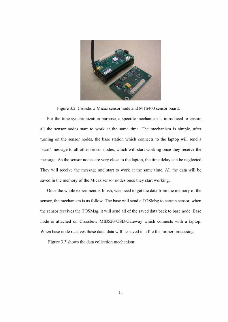
11
Figure 3.2 Crossbow Micaz sensor node and MTS400 sensor board.
For the time synchronization purpose, a specific mechanism is introduced to ensure
all the sensor nodes start to work at the same time. The mechanism is simple, after
turning on the sensor nodes, the base station which connects to the laptop will send a
‘start’ message to all other sensor nodes, which will start working once they receive the
message. As the sensor nodes are very close to the laptop, the time delay can be neglected.
They will receive the message and start to work at the same time. All the data will be
saved in the memory of the Micaz sensor nodes once they start working.
Once the whole experiment is finish, wee need to get the data from the memory of the
sensor, the mechanism is as follow. The base will send a TOSMsg to certain sensor, when
the sensor receives the TOSMsg, it will send all of the saved data back to base node. Base
node is attached on Crossbow MIB520-USB-Gateway which connects with a laptop.
When base node receives these data, data will be saved in a file for further processing.
Figure 3.3 shows the data collection mechanism:
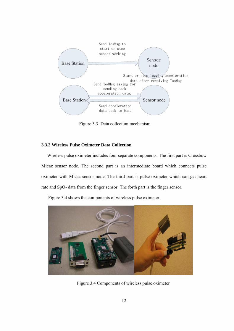
12
Base StationSensor node
Send TosMsg to start or stop
sensor working
Start or stop logging acceleration
data after receiving TosMsg
Base Station Sensor node
Send TodMsg asking for sending back
acceleration data.
Send acceleration data back to base
Figure 3.3 Data collection mechanism
3.3.2 Wireless Pulse Oximeter Data Collection
Wireless pulse oximeter includes four separate components. The first part is Crossbow
Micaz sensor node. The second part is an intermediate board which connects pulse
oximeter with Micaz sensor node. The third part is pulse oximeter which can get heart
rate and SpO2 data from the finger sensor. The forth part is the finger sensor.
Figure 3.4 shows the components of wireless pulse oximeter:
Figure 3.4 Components of wireless pulse oximeter
13
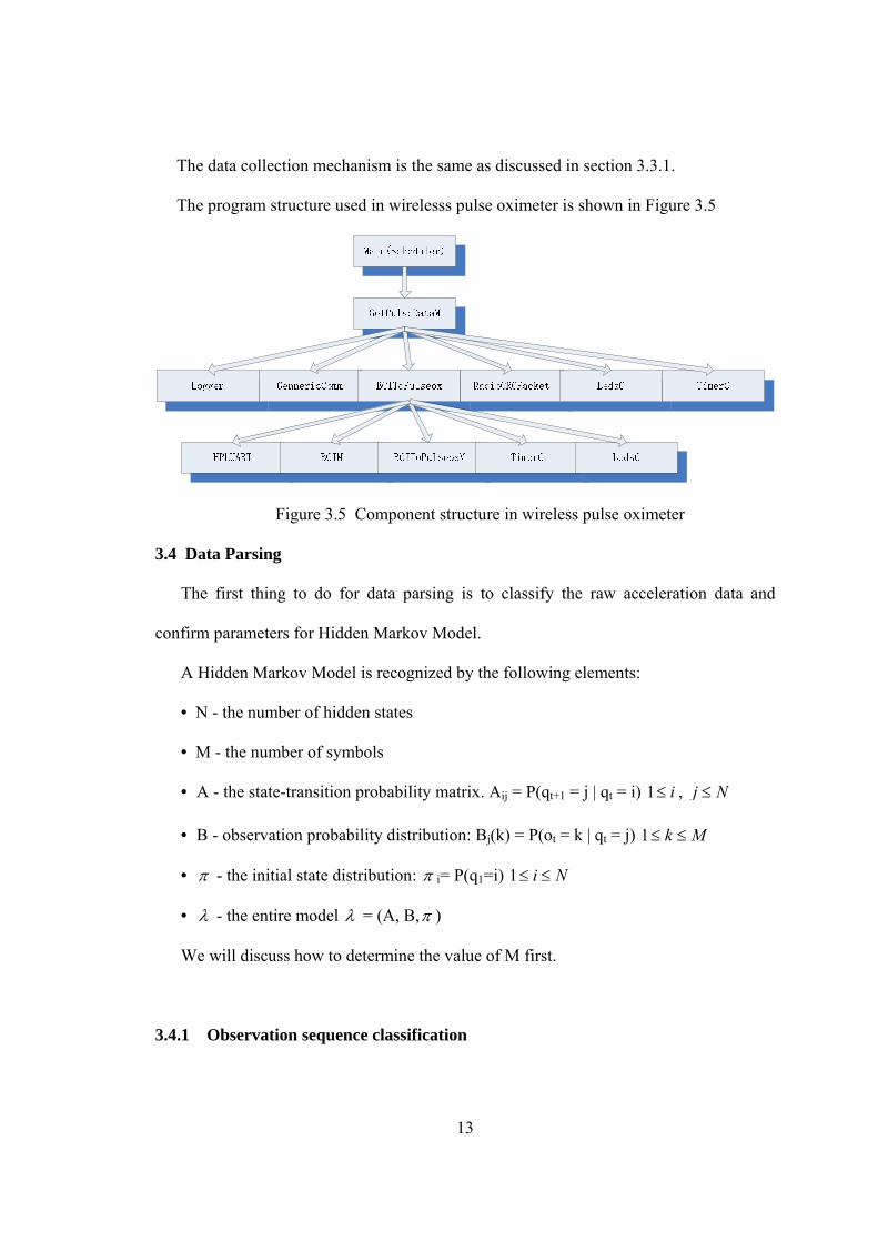
The data collection mechanism is the same as discussed in section 3.3.1.
The program structure used in wirelesss pulse oximeter is shown in Figure 3.5
Figure 3.5 Component structure in wireless pulse oximeter
3.4 Data Parsing
The first thing to do for data parsing is to classify the raw acceleration data and
confirm parameters for Hidden Markov Model.
A Hidden Markov Model is recognized by the following elements:
• N - the number of hidden states
• M - the number of symbols
• A - the state-transition probability matrix. Aij = P(qt+1 = j | qt = i) 1 i , j N
• B - observation probability distribution: Bj(k) = P(ot = k | qt = j) 1 k M
• - the initial state distribution: i= P(q1=i) 1 i N
• - the entire model = (A, B, )
We will discuss how to determine the value of M first.
3.4.1 Observation sequence classification

14
ADXL202E in MTS400 sensor board has x-axis and y-axis acceleration measurement.
Firstly, we need to get the resultant acceleration of X axis and Y axis:
2 2
xy x ya a a
The reason why we use resultant acceleration is that using either x-axis or y-axis data
alone will result in lower recognition rate for non-stationary human activities such as
climbing stairs, walking and running. In the other hand, we will use average value of x-
axis acceleration data when recognizing stationary activities as it will help to improve
recognition accuracy. Secondly, we group seven consecutive resultant acceleration data
together and calculate the value of following types of data in one group: a1, a2, and a3.
a1 means the maximum value minus the minimum value in one group for sensor one. a2
means the maximum value minus the minimum value in one group for sensor two. a3
means the maximum value minus the minimum value in one group for sensor three. But
a1, a2 and a3 are not the final observation symbols used in this thesis. There is one more
step to do for data processing. Thirdly, we will use a binary tree algorithm to classify a1,
a2, a3 values to different observation states.
The basic schema is shown in Figure 3.6:

15
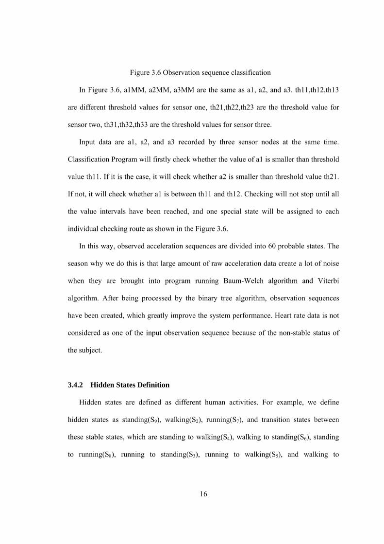
16
Figure 3.6 Observation sequence classification
In Figure 3.6, a1MM, a2MM, a3MM are the same as a1, a2, and a3. th11,th12,th13
are different threshold values for sensor one, th21,th22,th23 are the threshold value for
sensor two, th31,th32,th33 are the threshold values for sensor three.
Input data are a1, a2, and a3 recorded by three sensor nodes at the same time.
Classification Program will firstly check whether the value of a1 is smaller than threshold
value th11. If it is the case, it will check whether a2 is smaller than threshold value th21.
If not, it will check whether a1 is between th11 and th12. Checking will not stop until all
the value intervals have been reached, and one special state will be assigned to each
individual checking route as shown in the Figure 3.6.
In this way, observed acceleration sequences are divided into 60 probable states. The
season why we do this is that large amount of raw acceleration data create a lot of noise
when they are brought into program running Baum-Welch algorithm and Viterbi
algorithm. After being processed by the binary tree algorithm, observation sequences
have been created, which greatly improve the system performance. Heart rate data is not
considered as one of the input observation sequence because of the non-stable status of
the subject.
3.4.2 Hidden States Definition
Hidden states are defined as different human activities. For example, we define
hidden states as standing(S9), walking(S2), running(S7), and transition states between
these stable states, which are standing to walking(S4), walking to standing(S6), standing
to running(S8), running to standing(S3), running to walking(S5), and walking to
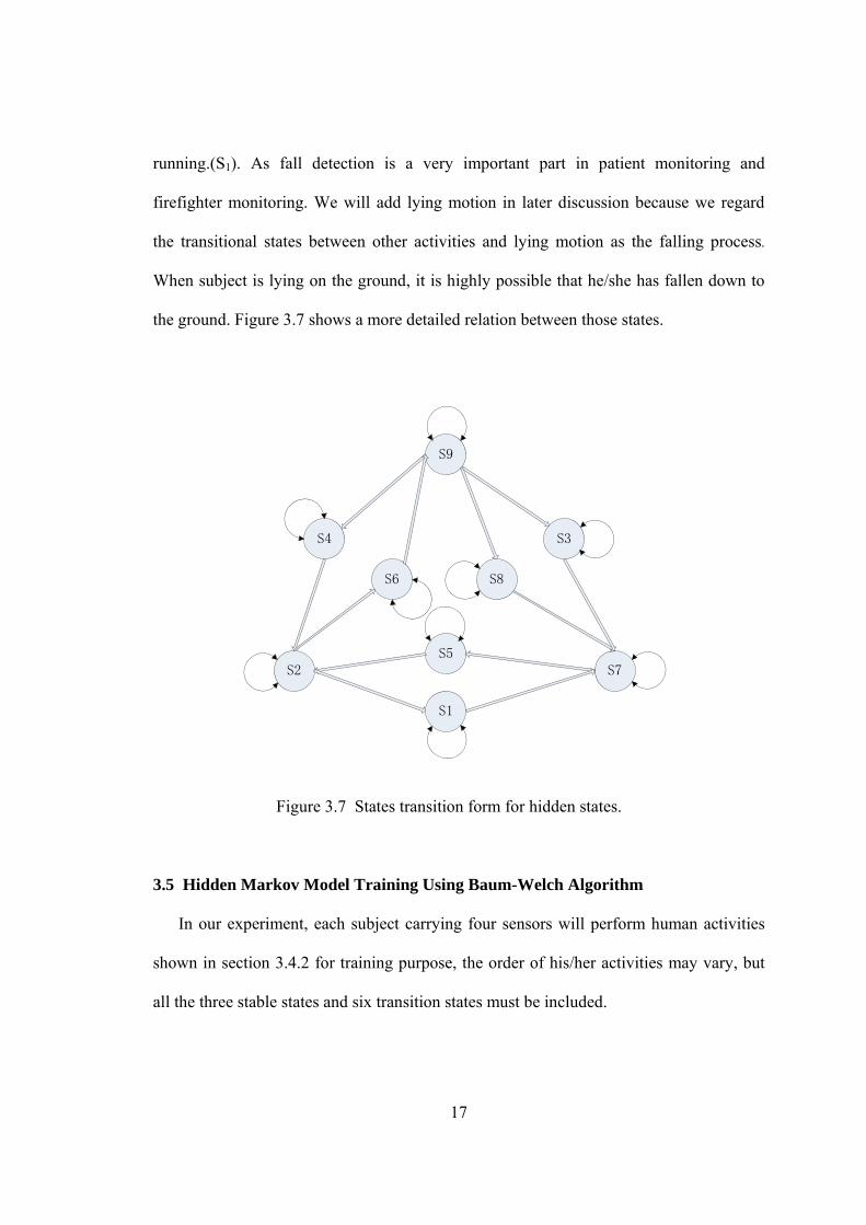
17
running.(S1). As fall detection is a very important part in patient monitoring and
firefighter monitoring. We will add lying motion in later discussion because we regard
the transitional states between other activities and lying motion as the falling process.
When subject is lying on the ground, it is highly possible that he/she has fallen down to
the ground. Figure 3.7 shows a more detailed relation between those states.
S9
S4
S6
S2
S3
S8
S7S5
S1
Figure 3.7 States transition form for hidden states.
3.5 Hidden Markov Model Training Using Baum-Welch Algorithm
In our experiment, each subject carrying four sensors will perform human activities
shown in section 3.4.2 for training purpose, the order of his/her activities may vary, but
all the three stable states and six transition states must be included.
18
3.5.1 Baum-Welch Algorithm
Baum-Welch algorithm is a GEM algorithm. GEM means generalized expectation-
maximization. It can compute maximum likelihood estimations and posterior mode
estimations for the parameters (transition and emission probabilities) of an HMM, when
given emission as the training data only.
The algorithm has two steps:
Firstly, calculating the forward probability and the backward probability for each
HMM state.
Secondly, calculating the transition-emission pair values and multiplied by the
probabilities of the whole observation sequence.
In another word, given O = (O1, O2,…, OT ); Estimate = (A,B, ) to maximize
P(O| ). The procedures of Baum-Welch Algorithm will be:
• Let initial model be 0
• Compute new based on 0 and observation O.
• If log P(O| ) - log P(O| 0) < , then stop.
• Else set 0 ← and go to the second step.
In [18], Baum et. al give a detailed explanation on the mathematical procedure how
this algorithm works.
Baum-Welch: Preliminaries:
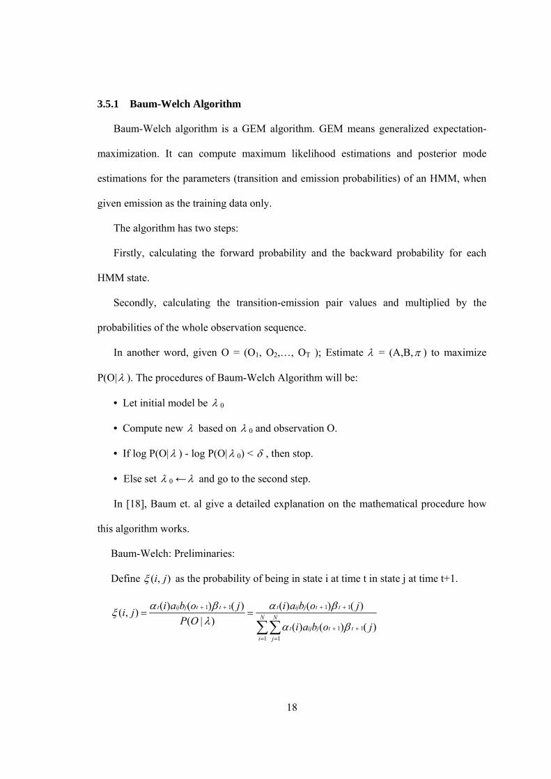
Define ( , )i j as the probability of being in state i at time t in state j at time t+1.
1 1 1 1
1 1
1 1
( ) ( ) ( ) ( ) ( ) ( )( , )
( | ) ( ) ( ) ( )
t ij j t t t ij j t t
N N
t ij j t t
i j
i a b o j i a b o ji j
P O i a b o j
19
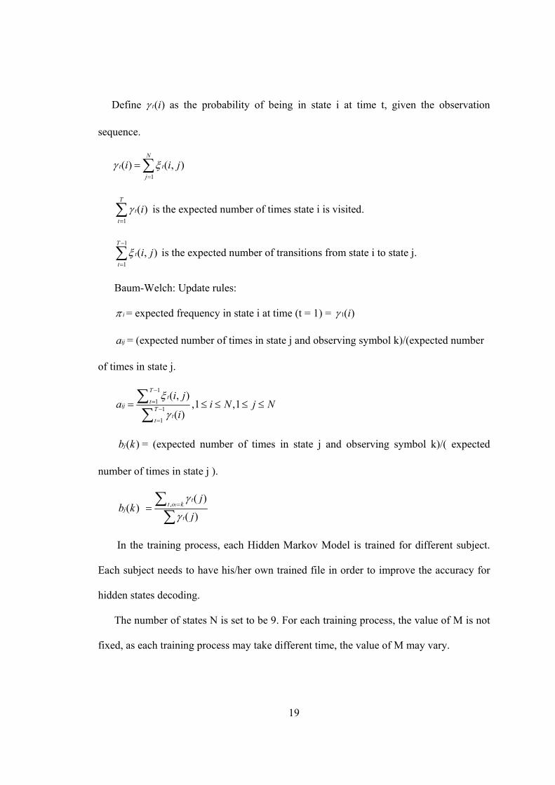
Define ( )t i as the probability of being in state i at time t, given the observation
sequence.
1
( ) ( , )N
t t
j
i i j
1
( )T
t
t
i is the expected number of times state i is visited.
1
1
( , )T
t
t
i j
is the expected number of transitions from state i to state j.
Baum-Welch: Update rules:
i = expected frequency in state i at time (t = 1) = 1( )i
ija = (expected number of times in state j and observing symbol k)/(expected number
of times in state j.
1
11
1
( , ),1 ,1
( )
Tt
tij T
tt
i ja i N j N
i
( )jb k = (expected number of times in state j and observing symbol k)/( expected
number of times in state j ).
( )jb k ,( )
( )t
tt o k
t
j
j
In the training process, each Hidden Markov Model is trained for different subject.
Each subject needs to have his/her own trained file in order to improve the accuracy for
hidden states decoding.
The number of states N is set to be 9. For each training process, the value of M is not
fixed, as each training process may take different time, the value of M may vary.

20
3.6 Hidden States Decoding
In this section, Viterbi algorithm is introduced to find the most probable activity
series (hidden states of HMM) from observation series.
The Viterbi algorithm is a dynamic programming algorithm to find the Viterbi path
that is hidden in the observed sequence. The Viterbi path can also be regarded as the most
likely sequence of hidden states. Assume to be the probability of the most probable
path to the state. Then ( )t i is the maximum probability of all possible sequences ending
at state i when it is time t. The Viterbi path is the sequence which results in this maximal
probability. A is the matrix of state-transition probabilities with elements aij, B is the
matrix of observation probabilities with elements bij, and is the vector of initial state
probabilities with elements (i). In mathematical expression:
Find the path (q1,…, qt ) that maximizes the likelihood P(q1,…, qt |O, ).
Solution by Dynamic Programming:
Define: 1 2 1
1 2 t 1 2,..., t, ,...,
( ) max (q ,q ...,q =i, o ,o o | )t
tq q q
i P
By induction we have:
1 1( ) max[ ( ) ] ( )t t ij j ti
j i a b o
Initialization:
1( ) ( ),1i i ii b o i N
1( ) 0i
Recursion:
1
1
( ) ( ) ] ( )max[t t ij j t
i N
j i a b o
11
( ) max[ ( ) ], 2 ,1t t iji N
j i a t T j N

21
Termination:
1max[ ( )]T
i NP i
*
1arg max[ ( )]TT
i Nq i
Path (state sequence) backtracking:
* *1 1( ), 1, 2,...,1tt tq q t T T
In the end, the Viterbi path will be calculated and we will discuss the hidden states decoding in later chapter.

22
CHAPTER 4
EXTENDED KALMAN FILTER IN INDOOR LOCALIZATION 4.1 Kalman Filter
Kalman filter is an efficient tool in estimating the state of a linear dynamic noisy
system. In the world of engineering, Kalman Filter plays an important role in many areas,
such as computer version, aerospace, aircraft navigation, control systems and so on. Most
famously, Kalman filter solves the linear-quadratic-Gaussian control problem (LQG) in
control theory. Kalman filter is based on the paper published in 1960 by R.E.Kalman,
who introduced a linear filtering method for discrete data. Kalman filter provides a good
estimate of the coming state according to the value of the previous state, which is
different from many other engineering filters, such as the Williams filter which requests
values from all the previous states. Kalman Filter estimates the state nx R of a discrete-
time controlled process described in the stochastic difference equation below:
1k k k kx A x Bx w
A measurement matrix mz R is provided for the estimation.
k k kz Hx v
Matrix A is a square matrix which relates the current process state estimate with the
state in the previous time instant. Matrix B is not necessarily a square matrix, and relates
the current process state estimate with the system input at previous time instance. Matrix
23
H, which is a rectangular matrix, relates measurement to state estimate. Variables wk-1
and vk are random variables representing the process noise and measurement noise. They
are assumed to be mutually independent, white and with normal probability distributions.
p(w) ~ N(0,Q)
p(v) ~ N(0,R)
Where Q is the process noise covariance and R is measurement noise covariance.
Although they are assumed to be zero, in reality, they change with each time update step
or measurement update step.
Kalman Filter is executed in two steps, which are time update and measurement
update. Time update projects the state variable vector estimate ahead with consideration
of the system input, which means that the time update function predicts the new state of
the Kalman Filter. The measurement update adjusts the time update estimation with
consideration of measurements during the time interval.
Kalman Filter is written as follow:
.. (4.1)
.. (4.2)
.. (4.3)
.. (4.4)
.. (4.5)
Firstly, we need to estimate the initial value of the state variable vector and error
covariance matrix. Then we need to go through following steps:
Step one: Time Update:
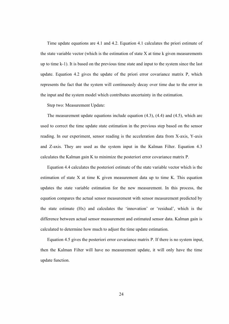
24
Time update equations are 4.1 and 4.2. Equation 4.1 calculates the priori estimate of
the state variable vector (which is the estimation of state X at time k given measurements
up to time k-1). It is based on the previous time state and input to the system since the last
update. Equation 4.2 gives the update of the priori error covariance matrix P, which
represents the fact that the system will continuously decay over time due to the error in
the input and the system model which contributes uncertainty in the estimation.
Step two: Measurement Update:
The measurement update equations include equation (4.3), (4.4) and (4.5), which are
used to correct the time update state estimation in the previous step based on the sensor
reading. In our experiment, sensor reading is the acceleration data from X-axis, Y-axis
and Z-axis. They are used as the system input in the Kalman Filter. Equation 4.3
calculates the Kalman gain K to minimize the posteriori error covariance matrix P.
Equation 4.4 calculates the posteriori estimate of the state variable vector which is the
estimation of state X at time K given measurement data up to time K. This equation
updates the state variable estimation for the new measurement. In this process, the
equation compares the actual sensor measurement with sensor measurement predicted by
the state estimate (Hx) and calculates the ‘innovation’ or ‘residual’, which is the
difference between actual sensor measurement and estimated sensor data. Kalman gain is
calculated to determine how much to adjust the time update estimation.
Equation 4.5 gives the posteriori error covariance matrix P. If there is no system input,
then the Kalman Filter will have no measurement update, it will only have the time
update function.

25
4.2 Extended Kalman Filter
Kalman Filter assumes that the relation between measurements, input and state
variables are all linear. This is not always the case as sometimes the system being
modeled can be a non-linear system. In that case, Extended Kalman Filter (EKF) is
introduced to solve the problem. For Extended Kalman Filter, the basic idea is to linearise
the non-linear measurement of current state estimation so that we can introduce similar
stochastic equation to perform the recursive procedures defined in Kalman Filter. With
this in mind, we will show the equations of EKF below:
..(4.6)
..(4.7)
This non-linear equation can be expressed by the linear equation:
..(4.8)
..(4.9)
Where:
A is the Jacobian matrix of partial derivatives of f with respect to x
H is the Jacobian matrix of partial derivatives of h with respect to x
W is the Jacobian matrix of partial derivatives of f with respect to w

26
V is the Jacobian matrix of partial derivatives of h with respect to v
The time update (predict) and measurement update (correct) equations are shown
below.
..(4.10)
..(4.11)
..(4.12)
..(4.13)
..(4.14)
4.3 Application of Extended Kalman Filter in Indoor Localization
4.3.1 RSSI Based distance measurement
Many localization algorithms request distance measurement to estimate the position
of unknown subject. Our algorithm will perform in the same manner. We use received
signal strength (RSSI) of the incoming radio signal to estimate distance between target
nodes and stable nodes. In our experiment, one sensor node will send message to another
sensor node with the transmission power PTX, and the receiver will have a receiving
power PRX which is a signal indicator that can be used for calculating the distance
between the transmitter and the receiver. PRX is directly effected by PTX
27
The radio model we use is described as below:
[ ] ( ) ( )i loss i i iP dBm P d t
Where:
100
( ) 10 logi
loss i TXd
P d P Kd
K is a unitless constant that depends on the environment. D0 is a reference distance
for the antenna far field, and is the path loss coefficient. i denotes the random
attenuation due to shadowing, while ( )i t accounts for the fast fading effect [37].
Therefore, the channel model can be combined as following equation:
100
[ ] 10 logi
i TX id
P dBm P Kd
..(4.15)
In our experiment we choose parameter value as K+PTX=-45dBm, =1.6, d0=1m,
i =6.82dBm. Then we have the expression of distance between the transmitter node and
the receiver node.
45.5 6.82
1610RSSI
d
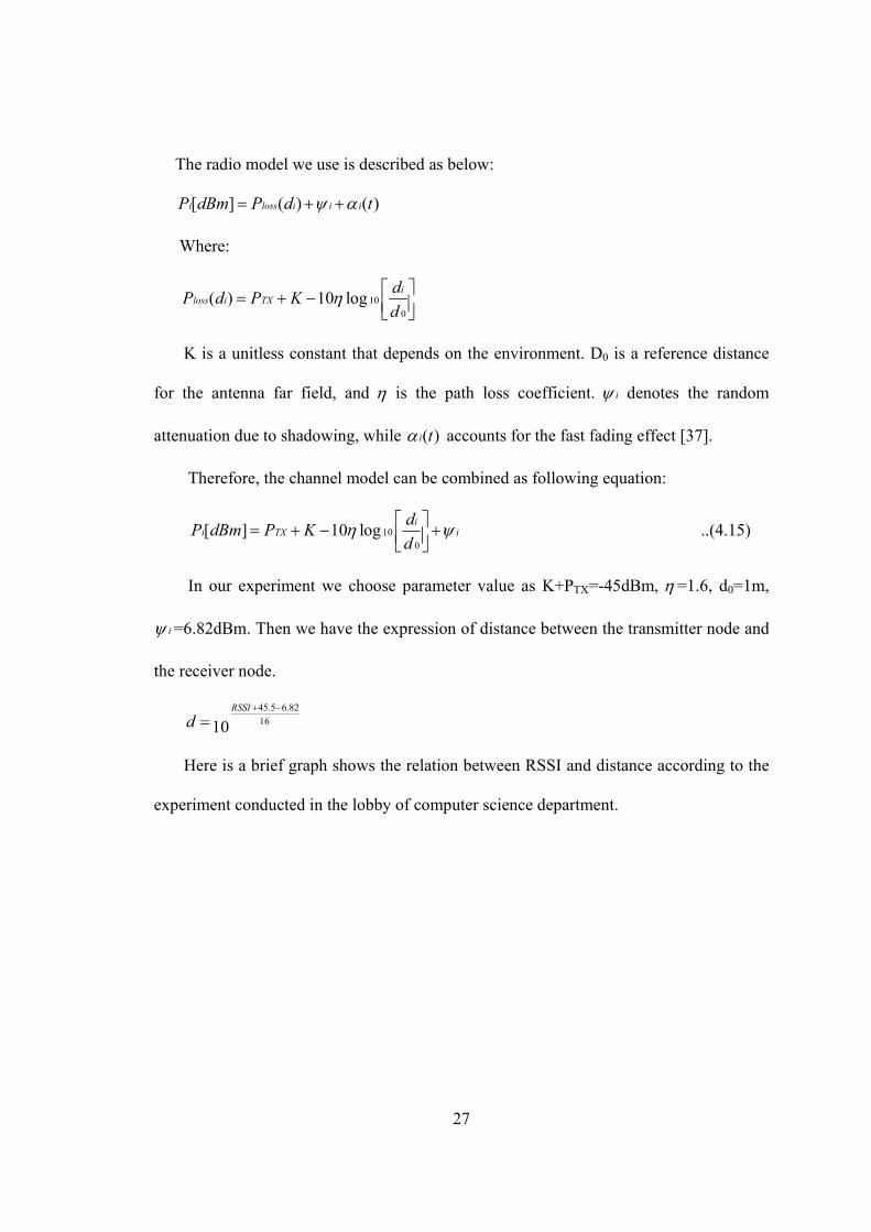
Here is a brief graph shows the relation between RSSI and distance according to the
experiment conducted in the lobby of computer science department.
28
Figure 4.1 Relation between distance and RSSI
4.3.2 System Model
The system consists of three stationary nodes deployed at pre-set coordinates. One
or two target nodes are carried by a human being. If acceleration data is not considered as
system input then only one target node is used. Otherwise, two nodes are used in order to
get x axis, y axis and z axis acceleration data as MTS400 sensor board can only measure
x axis and y axis acceleration data, we need to put one more sensor node to record z axis
acceleration data. In our experiment, direction of x axis is defined as pointing to the south
side, direction of y axis is defined as pointing to the west side and direction of z axis is
defined as pointing to ground. The target nodes will broadcast message to reference
nodes.
Assume that the coordinates of three stable nodes S1, S2 and S3 are (x1, y1, z1), (y2,
y2, z2) and (x3, y3, z3). The distance between stable nodes and target node are d1, d2, d3.
Then we can get the following equations:
29
2 2 2 21 1 1 1
2 2 2 22 2 2 2
2 2 2 23 3 3 3
( ) ( ) ( )
( ) ( ) ( )
( ) ( ) ( )
d x x y y z z
d x x y y z z
d x x y y z z
..(4.23--25)
We can get the calculated coordinate of target node using equation 4.23---4.25. This
result has very low accuracy in our experiment. d1, d2, d3 are measured by RSSI based
distance measurement method.
We can have three different system models according to how many states we want to
define in the EKF. Generally, we list three EKF models which relate to our subject
tracking project:
Coordinate Model: The state vector of EKF only contains the coordinate of the
subject.
Coordinate-Velocity Model: The state vector of EKF contains the coordinate of
subject and the moving speed of subject as well.
Coordinate-Velocity-Acceleration Model: The state vector of EKF contains
coordinate, speed and acceleration information of the subject.
We will use the third model here.
Let coordinate estimation vector be
x
y
z
x
y
z
x
y
z
v
X v
v
a
a
a

30
Where x, y, and z are the coordinate of target node. Vx, Vy and Vz are the velocity in x,
y and z axis. xa , ya and za are the acceleration in x, y and z axis.
The state space model is given as:
1
xk
k k yk k
zk
u
X AX B u X
u
Where
1 0 0 0 0 0 0 0
0 1 0 0 0 0 0 0
0 0 1 0 0 0 0 0
0 0 0 1 0 0 0 0 0
0 0 0 0 1 0 0 0 0
0 0 0 0 0 1 0 0 0
0 0 0 0 0 0 0 0 0
0 0 0 0 0 0 0 0 0
0 0 0 0 0 0 0 0 0
T
T
T
A
and
2
2
2
/ 2 0 0
0 / 2 0
0 0 / 2
0 0
0 0
0 0
1 0 0
0 1 0
0 0 1
T
T
T
T
B T
T
xku , yku , and zku are the control forces in x, y and z axis. kX is the system process
white noise.
Measurement equation can be described as shown below:
31
1 1 1
2 2 2
3 3 3
0 0 0 0 0 0
0 0 0 0 0 0
0 0 0 0 0 0
k k k k k
d d d
x y z
d d dZ HX Z X Z
x y z
d d d
x y z
Where:
2 2 2( ) ( ) ( )
i i
i i i
d x x
x x x y y z z
..(4.16)
2 2 2( ) ( ) ( )
i i
i i i
d y y
y x x y y z z
..(4.17)
2 2 2( ) ( ) ( )
i i
i i i
d z z
z x x y y z z
..(4.18)
Then according to the EKF algorithm, we will do the following calculation:
Step 1. Calculate 1k k kX A X BU
and kZ according to 1kX
.
Step 2. The error covariance equation is:
..(4.19)
Step 3. Compute the Kalman gain:
..(4.20)
Step 4. Update estimation with measurement function:
..(4.21)
Step 5. Update the error covariance:
..(4.22)
Step 6. Go to step 1.

32
CHAPTER 5
CONCLUSION AND FUTURE WORK
5.1 Human Activity Recognition Results
Once the Hidden Markov Models are built, three different series of human activities
are performed to have the models tested and find the Viterbi paths. They are:
1. Standing-walking-standing-climbing stairs-standing-running-standing
2. Standing-sitting-lying
3. Standing-walking-sitting-running-lying-walking-climbing stairs-walking-standing
Result graph is show as below. These results are based on the human activities
conducted by author himself.
For proposition one: Each subject will perform the following activities: standing,
walking, standing, climbing stairs, standing, running and standing.
standing-walking-standing-climing_stairs-standing-running-standing
0
2
4
6
8
10
12
1 11 21 31 41 51 61 71 81 91 101111121131141 151161
time(s)
Acceleration(m/s2)
toe sensor
shoulder sensor
leg sensor
Figure 5.1 Reluctant acceleration data for Proposition 1

33
Hidden States Decoding
0123456789
1 11 21 31 41 51 61 71 81 91 101111121131141151161
time(s)
Hidden States
Viterbi Path
Figure 5.2 Hidden States Decoding for Proposition 1.
In Figure 5.2, the meanings of hidden states are: standing(S6), walking(S2), climbing
stairs(S8), and running(S3). Transitional states include standing to walking, walking to
standing and so on. Hidden state S1 appears when subject moves from walking to
standing, standing to climbing stairs, and standing to running. So S1 can be regarded as
the transitional state. As S1 is supposed to have only one definition, the transitional states
are not well recognized in this graph. Other transitional states in this figure include S4 and
S5. X-axis represents time, y-axis represents the hidden states.
Figure 5.1 shows the original reluctant sensor data a1, a2, and a3, which we
mentioned in section 3.4.1. Series 1 stands for the sensor node placed at the left toe.
Series 3 stands for the sensor node placed at the right leg. Series 2 stands for the sensor
node placed at the right side of waist. Human activities performed in the first graph are
clearly recognized as shown in the second graph. X-axis represents time and y-axis
represents acceleration with unit m/s^2. Time unit is 1 second.
For proposition 2, each subject will go through standing, sitting and lying activities.
34
standing-sitting-lying
0
0.5
1
1.5
2
2.5
1 13 25 37 49 61 73 85 97 109 121 133 145 157
time(s)
Acceleration(m/s2)
toe sensor
chest sensor
leg sensor
Figure 5.4 Reluctant acceleration data for Proposition 2.
Hidden States Decoding
0
1
2
3
4
5
6
7
1 13 25 37 49 61 73 85 97 109 121 133 145 157
time(s)
Hidden States
Viterbi Path
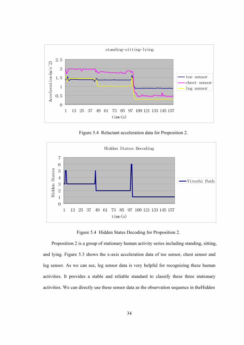
Figure 5.4 Hidden States Decoding for Proposition 2.
Proposition 2 is a group of stationary human activity series including standing, sitting,
and lying. Figure 5.3 shows the x-axis acceleration data of toe sensor, chest sensor and
leg sensor. As we can see, leg sensor data is very helpful for recognizing these human
activities. It provides a stable and reliable standard to classify these three stationary
activities. We can directly use these sensor data as the observation sequence in theHidden

35
Markov Model without running the classification algorithm. In Figure 5.3, as those
human activities are stationary, our accelerometers are supposed to have zero reading.
But we still get different sensor reading from accelerometers, which is because of the
drift of the accelerometers. We will not use the calibrated acceleration data here, instead,
we use the drift of accelerometers as a better indicator for stationary activities. When
considering about the combination of stationary and non-stationary human activities, we
will do the calibration in order to get the correct result. But the X-axis acceleration data
will also be taken into account in the classification algorithm when classifying combined
activities. X-axis represents time, with one second as the unit, Y-axis represents
acceleration, with m/s^2 as the unit. In Figure 5.4, Hidden states are defined as
standing(S3), sitting(S2), and lying(S1). We recall that standing is defined as S6 in
proposition 1, which is different from proposition 2. The reason is that we use different
Hidden Markov Model for the hidden states decoding. With different models, hidden
states are given different symbol numbers. The hidden states are well recognized in
Figure 5.4.
In proposition 3, each subject will go through standing, walking, sitting, running,
lying, climbing stairs, and standing which is a combination of stationary and non-
stationary human activities.

36
standing-walking-sitting-running-lying-climbing stairs-standing
012345678
1 16 31 46 61 76 91 106121 136151166181 196
time(s)
Acceleration(m/s2)
toe sensor
waist sensor
leg sensor
Figure 5.5 Reluctant acceleration data for Proposition 3
Hidden States Decoding
0
1
2
3
4
5
6
7
8
1 16 31 46 61 76 91 106121 136151 166181 196211
time(s)
Hidden States
Viterbi Path
Figure 5.6 Hidden States Decoding for Proposition 3.
In Figure 5.5, we can see that the reluctant data is 0 for stationary motion. So we will
use X-axis acceleration data from leg sensor in our recognition process. In Figure 5.6,
experiment shows the accuracy of recognizing climbing stairs is not as high as walking
and running, which can be observed from the Figure 5.5, acceleration data for climbing
stairs becomes fuzzy in the middle of the climbing activity.

37
Hidden states are defined to be different symbols in different experiments because of
different Hidden Markov Models being used. In proposition 3, they are defined as
standing(S3), walking(S6), sitting(S4), running(S1), lying(S2), and climbing stairs(S5).
In Figure 5.6, at the end of running activity, subject fell down and laid on the ground,
at the same time, hidden state goes from S2 to S5, then to S3. Fall detection can be
introduced by recognizing these sudden changes.
0
20
40
60
80
100
120
standing sitting lying walking running climbingstairs
Accuracy(%)
HMM
non-HMM
Figure 5.7 Accuracy of human activities recognition with HMM and without HMM
Figure 5.7 compares the accuracy of human activities recognition with HMM and
without HMM (using collected acceleration data directly). As we can see, HMM greatly
improve the accuracy of human activities recognition rate. For stationary activities
(standing, sitting, lying), we achieve 100 percent accuracy. For non-stationary activities,
we achieve comparably lower accuracy, as acceleration data are not stable and changes
from time to time. Even though, it is still much better than using the acceleration data
directly. Raw data can hardly be used for determining what the subject is doing at
38
specific moment. The graph is plotted based on subject mounted with three sensors which
are deployed at left toe, right leg and right waist.
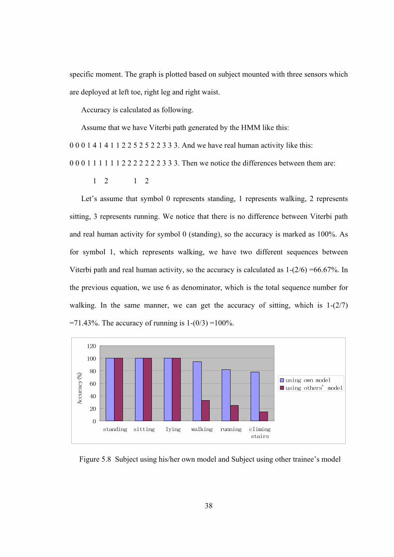
Accuracy is calculated as following.
Assume that we have Viterbi path generated by the HMM like this:
0 0 0 1 4 1 4 1 1 2 2 5 2 5 2 2 3 3 3. And we have real human activity like this:
0 0 0 1 1 1 1 1 1 2 2 2 2 2 2 2 3 3 3. Then we notice the differences between them are:
1 2 1 2
Let’s assume that symbol 0 represents standing, 1 represents walking, 2 represents
sitting, 3 represents running. We notice that there is no difference between Viterbi path
and real human activity for symbol 0 (standing), so the accuracy is marked as 100%. As
for symbol 1, which represents walking, we have two different sequences between
Viterbi path and real human activity, so the accuracy is calculated as 1-(2/6) =66.67%. In
the previous equation, we use 6 as denominator, which is the total sequence number for
walking. In the same manner, we can get the accuracy of sitting, which is 1-(2/7)
=71.43%. The accuracy of running is 1-(0/3) =100%.
0
20
40
60
80
100
120
standing sitting lying walking running climingstairs
Accuracy(%)
using own model
using others' model
Figure 5.8 Subject using his/her own model and Subject using other trainee’s model
39
When we apply the training file of one user to get the Viterbi path of another user,
result is shown in Figure 5.8. As we can see, recognition accuracy drops dramatically for
non-stationary human activities. So we need to train the HMM specifically for each
subject in order to get optimal recognition result.
0
20
40
60
80
100
120
standing sitting lying walking running climbingstairs
Accuracy(%)
one sensor
two sensors
three sensors
Figure 5.9 Comparison of accuracy for human activities with one sensor, two sensors
and three sensors mounted on each subject
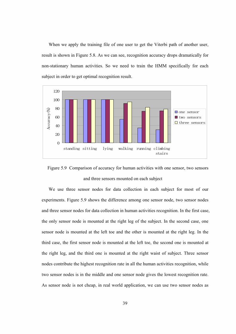
We use three sensor nodes for data collection in each subject for most of our
experiments. Figure 5.9 shows the difference among one sensor node, two sensor nodes
and three sensor nodes for data collection in human activities recognition. In the first case,
the only sensor node is mounted at the right leg of the subject. In the second case, one
sensor node is mounted at the left toe and the other is mounted at the right leg. In the
third case, the first sensor node is mounted at the left toe, the second one is mounted at
the right leg, and the third one is mounted at the right waist of subject. Three sensor
nodes contribute the highest recognition rate in all the human activities recognition, while
two sensor nodes is in the middle and one sensor node gives the lowest recognition rate.
As sensor node is not cheap, in real world application, we can use two sensor nodes as
40
their recognition rate is not significant lower than three sensor nodes. But these two
sensor nodes must be mounted on toe and leg of the subject.
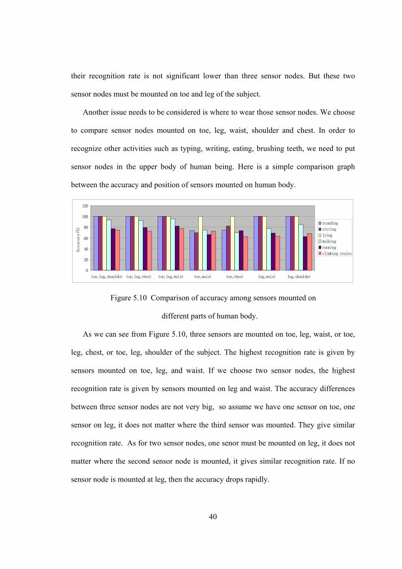
Another issue needs to be considered is where to wear those sensor nodes. We choose
to compare sensor nodes mounted on toe, leg, waist, shoulder and chest. In order to
recognize other activities such as typing, writing, eating, brushing teeth, we need to put
sensor nodes in the upper body of human being. Here is a simple comparison graph
between the accuracy and position of sensors mounted on human body.
0
20
40
60
80
100
120
toe,leg,shoulder toe,leg,chest toe,leg,waist toe,waist toe,chest leg,waist leg,shoulder
Accuracy(%) standing
sitting
lying
walking
running
climbing stairs
Figure 5.10 Comparison of accuracy among sensors mounted on
different parts of human body.
As we can see from Figure 5.10, three sensors are mounted on toe, leg, waist, or toe,
leg, chest, or toe, leg, shoulder of the subject. The highest recognition rate is given by
sensors mounted on toe, leg, and waist. If we choose two sensor nodes, the highest
recognition rate is given by sensors mounted on leg and waist. The accuracy differences
between three sensor nodes are not very big, so assume we have one sensor on toe, one
sensor on leg, it does not matter where the third sensor was mounted. They give similar
recognition rate. As for two sensor nodes, one senor must be mounted on leg, it does not
matter where the second sensor node is mounted, it gives similar recognition rate. If no
sensor node is mounted at leg, then the accuracy drops rapidly.
41
From the result we discussed before, it is clear that Hidden Markov Model gives an
outstanding performance in human activities recognition.
5.2 Indoor Localization Results
5.2.1 Experiment Set-up
Several experiments were conducted in computer science department.
First experiment: Three stable nodes were deployed at different places along the lobby
at computer science department. Their coordinates are given as (0, 0, 0), (0.9, 1.2, 0) and
(0, 1.8, 0.6). Test bed is set to be a 1.8m*2.1m*1.5m area. Two target nodes were
mounted together vertically on the subject. One target node recorded the acceleration of x
axis and y axis. The other target node recorded acceleration of z axis. Both of the target
nodes had been calibrated before they were used. The experiment result shows that the
longer the distance, the worse the accuracy will be. In the first experiment, one subject
will walk diagonally from one side to the other side of the area.
The mechanism of data collection is simple. Firstly, turn on the stable nodes. They
will wait for the message sent from target nodes. Secondly, turn on the target nodes.
Thirdly, send a TOS message from base station to target nodes. After receiving the
message, both of the target nodes will record the acceleration data in a fixed time interval.
At the same time, one of the target nodes will send another TOS message which contains
the transmission power value to the stable nodes. When stable nodes receive the message
from target node, they will record the RSSI value of received message and send a TOS
message containing RSSI value and transmission power to base station. A java program
running in the base station will process the raw data for distance calculation and EKF
42
based optimization.
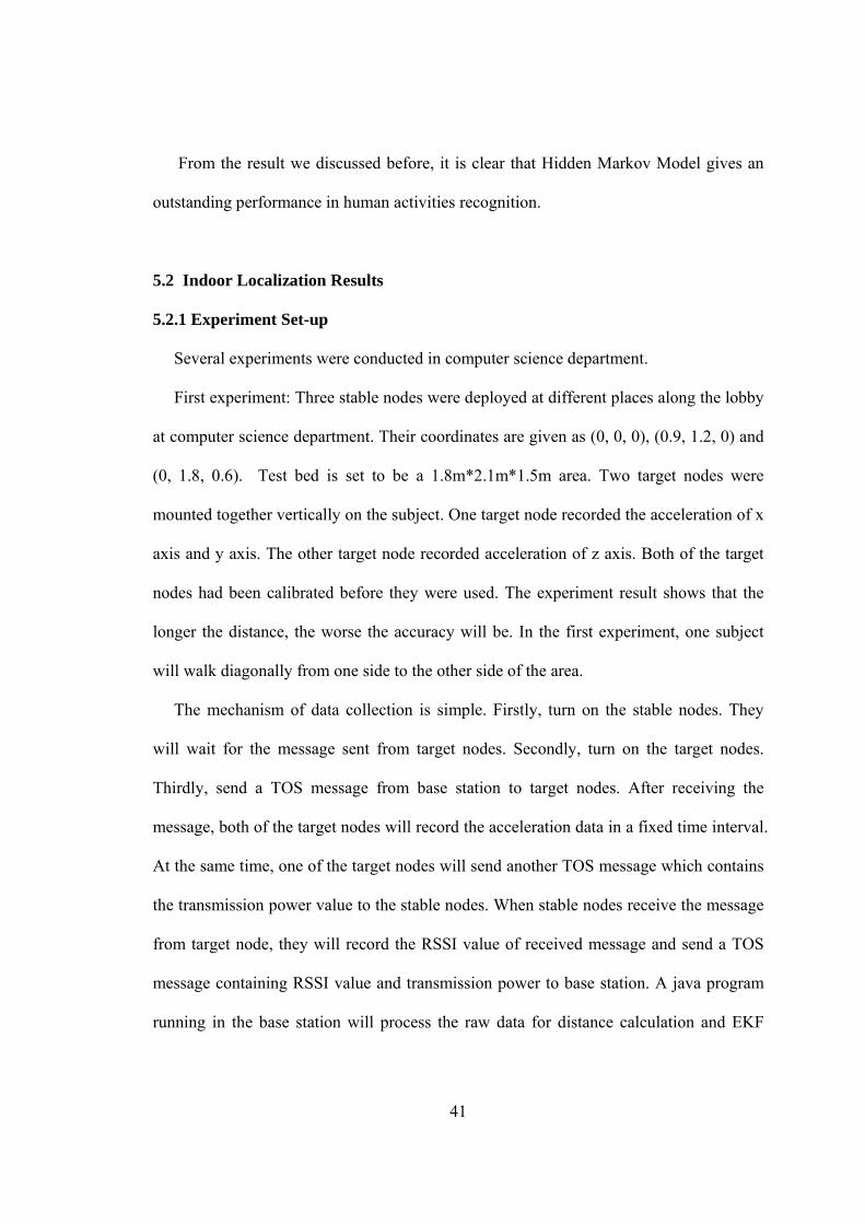
Figure 5.11 Two target nodes deployed vertically to record three axis acceleration data
5.2.2 Experiment Results
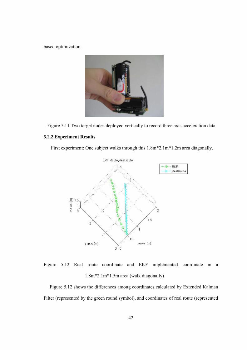
First experiment: One subject walks through this 1.8m*2.1m*1.2m area diagonally.
Figure 5.12 Real route coordinate and EKF implemented coordinate in a
1.8m*2.1m*1.5m area (walk diagonally)
Figure 5.12 shows the differences among coordinates calculated by Extended Kalman
Filter (represented by the green round symbol), and coordinates of real route (represented
43
by the light blue rectangle). As we can see, EKF performs well in measuring the distance
that subject traveled in three axis. The longer the subject walks, the bigger the
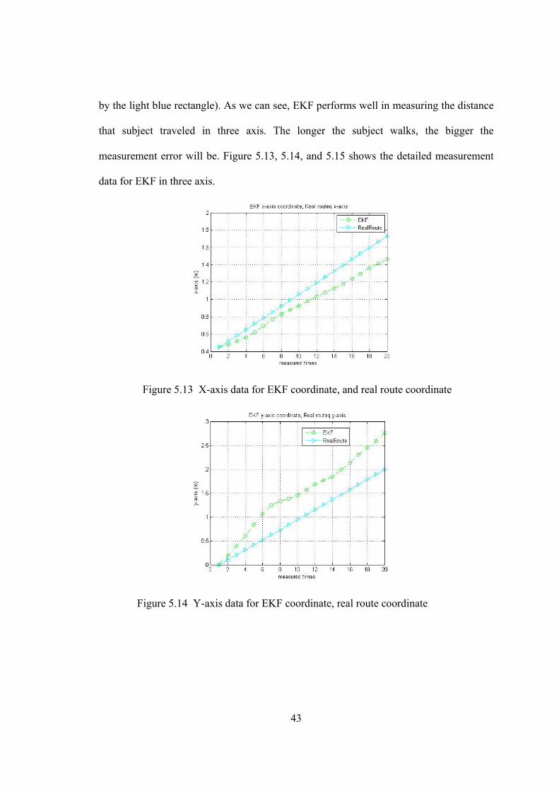
measurement error will be. Figure 5.13, 5.14, and 5.15 shows the detailed measurement
data for EKF in three axis.
Figure 5.13 X-axis data for EKF coordinate, and real route coordinate
Figure 5.14 Y-axis data for EKF coordinate, real route coordinate
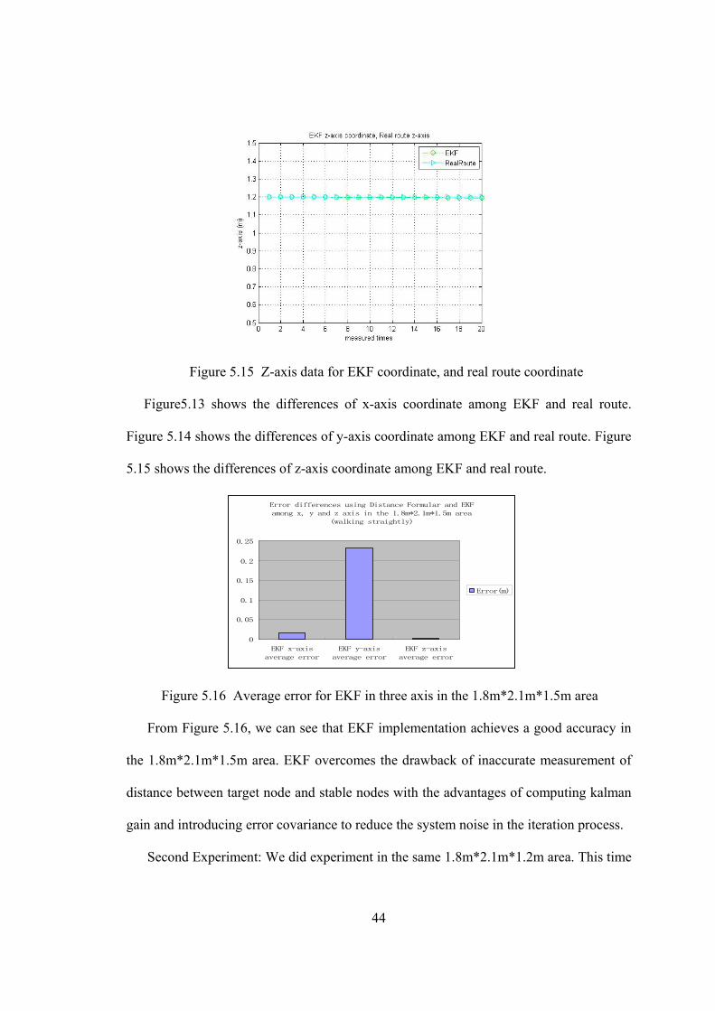
44
Figure 5.15 Z-axis data for EKF coordinate, and real route coordinate
Figure5.13 shows the differences of x-axis coordinate among EKF and real route.
Figure 5.14 shows the differences of y-axis coordinate among EKF and real route. Figure
5.15 shows the differences of z-axis coordinate among EKF and real route.
Error differences using Distance Formular and EKF
among x, y and z axis in the 1.8m*2.1m*1.5m area
(walking straightly)
0
0.05
0.1
0.15
0.2
0.25
EKF x-axis
average error
EKF y-axis
average error
EKF z-axis
average error
Error(m)
Figure 5.16 Average error for EKF in three axis in the 1.8m*2.1m*1.5m area
From Figure 5.16, we can see that EKF implementation achieves a good accuracy in
the 1.8m*2.1m*1.5m area. EKF overcomes the drawback of inaccurate measurement of
distance between target node and stable nodes with the advantages of computing kalman
gain and introducing error covariance to reduce the system noise in the iteration process.
Second Experiment: We did experiment in the same 1.8m*2.1m*1.2m area. This time
45
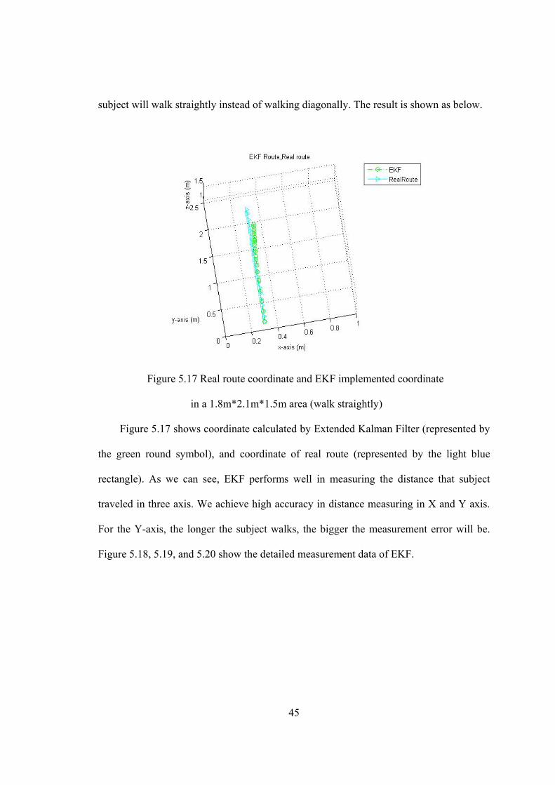
subject will walk straightly instead of walking diagonally. The result is shown as below.
Figure 5.17 Real route coordinate and EKF implemented coordinate
in a 1.8m*2.1m*1.5m area (walk straightly)
Figure 5.17 shows coordinate calculated by Extended Kalman Filter (represented by
the green round symbol), and coordinate of real route (represented by the light blue
rectangle). As we can see, EKF performs well in measuring the distance that subject
traveled in three axis. We achieve high accuracy in distance measuring in X and Y axis.
For the Y-axis, the longer the subject walks, the bigger the measurement error will be.
Figure 5.18, 5.19, and 5.20 show the detailed measurement data of EKF.

46
Figure 5.18 X-axis coordinate of EKF, and real route
Figure 5.19 Y-axis coordinate of EKF, and real route

47
Figure 5.20 Z-axis coordinate of EKF, and real route
From Figure 5.18, 5.19 and 5.20, we can see that EKF gives a precise estimation of
moving subject in X-axis and Z-axis, but in Y-axis, the estimation is not as precise as X-
axis and Y-axis. The experiment result shows that if the acceleration in one axis does not
change too much when the subject is moving, then the accuracy in certain axis can be
improved. In the second experiment, subject walks straightly on Y-axis, and the
environment noise is comparably larger on Y-axis. In the EKF model, we can adjust
different parameters in order to get better measurement result. We can use different
environment noise value to optimize the measurement result. When we applied it to the
real world application, we may need to figure out how to adjust parameters from time to
time in order to get better estimation for the subject localization.
Error differences using Distance Formular and EKF
among x, y and z axis in the 1.8m*2.1m*1.5m area
(walking straightly)
0
0.05
0.1
0.15
0.2
0.25
EKF x-axis
average error
EKF y-axis
average error
EKF z-axis
average error
Error(m)
Figure 5.21 Average error for EKF in three axis in the 1.8m*2.1m*1.5m area
Figure 5.21 shows the similar result with Figure 5.16, but X-axis error has been
greatly reduced.
Third Experiment: This time we did experiment in a larger area which is
1.8m*6m*1.5m. All the mechanism being used in the third experiment is the same as in
the first and second experiment.
48
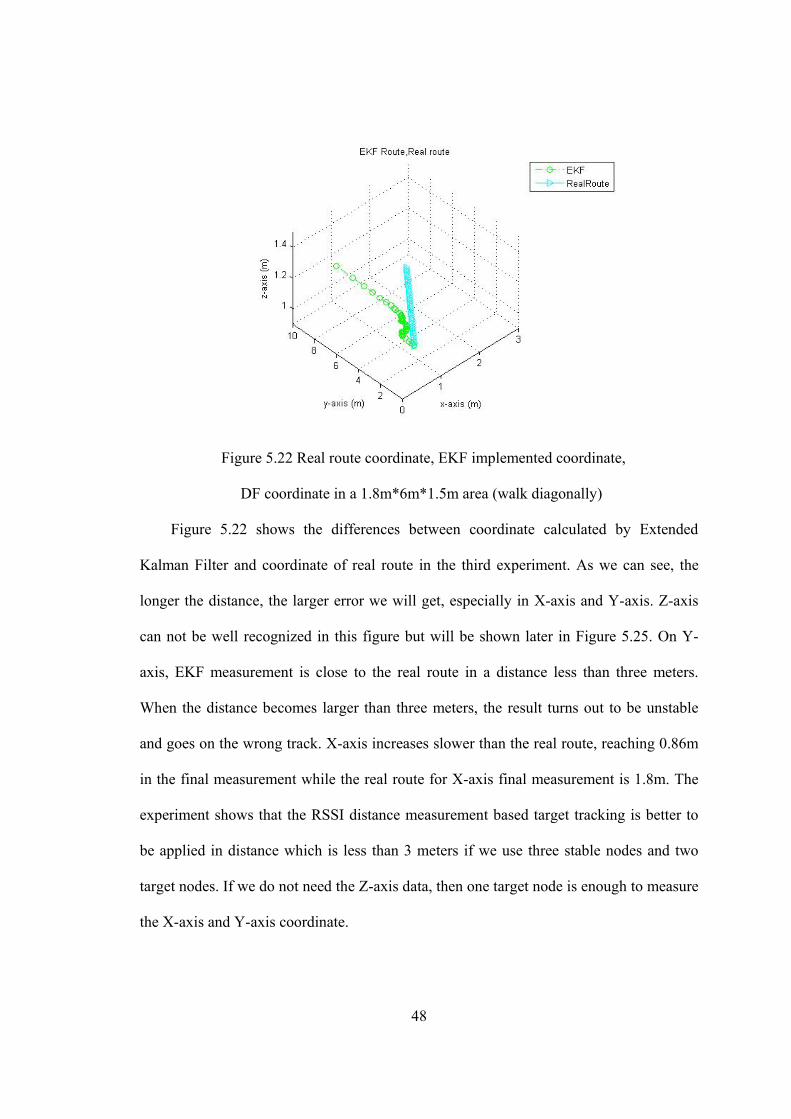
Figure 5.22 Real route coordinate, EKF implemented coordinate,
DF coordinate in a 1.8m*6m*1.5m area (walk diagonally)
Figure 5.22 shows the differences between coordinate calculated by Extended
Kalman Filter and coordinate of real route in the third experiment. As we can see, the
longer the distance, the larger error we will get, especially in X-axis and Y-axis. Z-axis
can not be well recognized in this figure but will be shown later in Figure 5.25. On Y-
axis, EKF measurement is close to the real route in a distance less than three meters.
When the distance becomes larger than three meters, the result turns out to be unstable
and goes on the wrong track. X-axis increases slower than the real route, reaching 0.86m
in the final measurement while the real route for X-axis final measurement is 1.8m. The
experiment shows that the RSSI distance measurement based target tracking is better to
be applied in distance which is less than 3 meters if we use three stable nodes and two
target nodes. If we do not need the Z-axis data, then one target node is enough to measure
the X-axis and Y-axis coordinate.
49
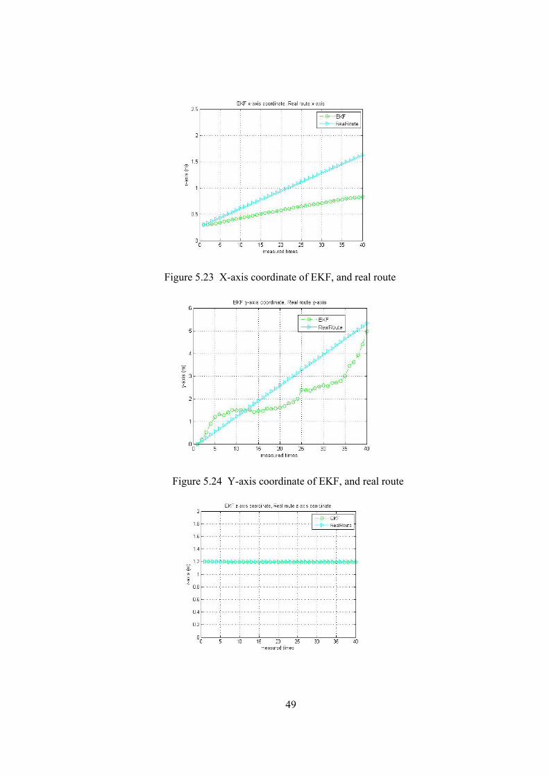
Figure 5.23 X-axis coordinate of EKF, and real route
Figure 5.24 Y-axis coordinate of EKF, and real route

50
Figure 5.25 Z-axis coordinate of EKF, and real route
From Figure 5.23, 5.24 and 5.25, we get a better understanding about the
performance of EKF on X-axis, Y-axis and Z-axis measurement.
Error differences using Distance Formular and EKF
among x, y and z axis in the 1.8m*6m*1.5m area
(walking diagnally)
0
0.1
0.2
0.3
0.4
0.5
0.6
0.7
0.8
0.9
1
EKF x-axis
average error
EKF y-axis
average error
EKF z-axis
average error
Error(m) s
Error(m)
Figure 5.26 Average error for EKF in three axis in the 1.8m*6m*1.5m area
As we can see from Figure 5.26, the accuracy of X-axis and Y-axis are decreasing
sharply compared to accuracy result shown on Figure 5.21. In order to get a better
estimation result, we need to deploy more stable nodes along the route of the subject .
From experiment one, two and three, we compare three different walking activities
which are walking diagonally, walking straightly, and walking diagonally in a larger area.
We can see that EKF gives a good estimation for indoor localization when the subject
moves in a 1.8m*2.1m*1.5m area. Further movement to a longer distance such as 6
meters in Y-axis will result in inaccurate measurement result. More research on
environment noise parameters of Extended Kalman Filter is needed in order to apply
EKF in a longer distance measurement and more human activities involved (as we only
did the walking experiment in this thesis). More sensor nodes are needed to provide
larger scale subject localization as well.
51
5.3 Conclusion and Future Work
In this thesis, three different human activity series have been tested. Hidden Markov
Model has been proved to be an effective tool in human activity recognition. We
achieved a high recognition rate on both stationary and non-stationary activities. We
discuss where to deploy the sensor nodes on human body and how many sensor nodes are
enough for monitoring the activities we performed in our lab. We also show that
individual training is compulsory in order to have a better recognition rate for the subject.
Fall detection has been briefly discussed, which takes the lying activity into account.
Future work may relate to recognize more human activities, such as reading, writing,
typing, eating, jumping and so on. A more flexible mechanism needs to be introduced for
real time monitoring which has more system restriction and system noise than the
experiment conducted in our lab.
Extended Kalman Filter (EKF) is introduced in indoor localization section.
Experiment result shows that EKF can effectively improve the accuracy of sensor
measurement in a 1.8m*2.1m*1.5m area. As for the 1.8m*6m*1.5m area, error rates
from EKF grows, which may be caused by the inaccurate measurement of distance
between target nodes and stable nodes based on RSSI. Future work may relate to
introduce more sensor nodes in the experiment for larger scale localization. Besides, the
experiment we did is to get absolute coordinate of the sensor node. In the real world
application, such as indoor localization for firefighters, when firefighters are on duty, we
can not deploy stable nodes in advance in the building where they are on mission. In that
case, we need to calculate the relative coordinate for each firefighter, so that once danger
happens to one firefighter, he/she can get help from his/her companion according to the

52
relative location calculated by the sensor node.
53
REFERENCES
[1] Rafael David Kaliski “Tinyos Laboratory Develepment”
[2] T. Zimmerman, “Personal area networks: near-field intrabody communication,” IBM
systems Journal, 1996, vol. 35, no. 3 & 4, pp. 609-617.
[3] D. Malan, T. Fulford-Jones, M. Welsh, and S. Moulton. “Codeblue: An ad hoc sensor
network infrastructure for emergency medical care.” In Proc. of the International
Workshop on Wearable and Implanatable Body Sensor Networks, April 2004.
[4] M. J. Mathie, A. C. F. Coster, N. H. Lovell, and B. G. Celler: “Accelerometry:
Providing an Integrated, Practical Method for Long-term, Ambulatory Monitoring of
Human Movement”, Physiological Measurement, 25. R1-R20. 2004.
[5] Harvard Sensor Network Lab http://fiji.eecs.harvard.edu/CodeBlue
[6] Ossama Younis and Sonia Fahmy, "An Experimental Study of Routing and Data
Aggregation in Sensor Networks," In Proceedings of the International Workshop on
Localized Communication and Topology Protocols for Ad hoc Networks (LOCAN), held
in conjunction with The 2nd IEEE International Conference on Mobile Ad Hoc and
Sensor Systems (MASS-2005), November 2005.
[7] Seon-Woo Lee and Kenji Mase. “Activity and location recognition using wearable
sensors.” IEEE Pervasive Computing, 1(3):24–32, 2002.
[8] K. Takenoshita, N. Shiozawa, J. Onishi and M. Makikawa, “Development of a
Portable Acceleration Monitor Device and its clinical application for the Quantitative
Gait Assessment of the Elderly”. Proceedings of the 2005 IEEE Engineering in Medicine

54
and Biology 27th Annual Conference Shanghai, China, September 1-4, 2005
[9] Michael Sung, Carl Marci and Alex Pentland, “Wearable feedback systems for
rehabilitation,” Journal of NeuroEngineering and Rehabilitation, Vol.2, No.17, June 2005
[10] J. Mantyjarvi, J. Himberg, and T. Seppanen. “Recognizing human motion with
multiple acceleration sensors,” In Proceedings of the IEEE International Conference
on Systems, Man, and Cybernetics, pages 747–52. IEEE Press, 2001.
[11] M. Makikawa, S. Kurata, Y. Higa, Y. Araki, and R. Tokue. “Ambulatory monitoring
of behavior in daily life by accelerometers set at both-near-sides of the joint,” In
Proceedings of Medinfo, volume 10(Pt) 1, pages 840–3. 2001.
[12] B. Clarkson and A. Pentland. “Predicting daily behavior via wearable sensors,”
Technical report, Massachusetts Institute of Technology Media Laboratory, July 2001.
[13] J. B. Bussmann, W. L. Martens, J. H. Tulen, F. C. Schasfoort, H. J. van den Berg-
Emons, and H. J. Stam. “Measuring daily behavior using ambulatory accelerometry: the
activity monitor,” Behavior Research Methods, Instruments, & Computers, 33(3):349–56,
2001.
[14] G. S. Chambers, S. Venkatesh, G. A. W.West, and H. H. Bui. “Hierarchical
recognition of intentional human gestures for sports video annotation,” In International
Conference on Pattern Recognition, pages 1082–5, Quebec City, 2002.
[15] L.E. Baum and T. Petrie, “Statistical Inference for Probabilistic Functions of Finite
State Markov Chains,” Annals of Math. Statistics, vol. 37, pp. 1,554-1,563, 1966.
[16] L.E. Baum and J.A. Egon, “An Inequality with Applications to Statistical
Estimation for Probabilistic Functions of a Markov Process and to a Model for Ecology,”
Bull. Amer. Meteorology Soc., vol. 73, pp. 360-363, 1967.
55
[17] L.E. Baum, G.R. Sell, “Growth Functions for Transformations on Manifolds,”
Pacific J. Math., vol. 27, no. 2, pp. 211-227, 1968.
[18] L.E. Baum, T. Petrie, G. Soules, and N. Weiss, “A Maximization Technique
Occurring in the Statistical Analysis of Probabilistic Functions of Markov Chains,”
Annals of Math. Statistics, vol. 41, no. 1, pp. 164-171, 1970.
[19] L. Baum, “An Inequality and Associated Maximization Technique in Statistical
Estimation for Probabilistic Functions of Markov Processes,” Inequalities, vol. 3, pp. 1-8,
1970.
[20] C.F.J. Wu, “On the Convergence Properties of the EM Algorithm,” Annals of
Statistics, vol. 11, no. 1, pp. 95-103, 1983.
[21] S.E. Levinson, L.R. Rabiner, and M.M. Sondhi, “An Introduction to the Application
of the Theory of Probabilistic Functions of Markov Process to Automatic Speech
Recognition,” Bell System Technical J., vol. 62, no. 4, pp. 1,035-1,074, 1983.
[22] G. Rigoll, A. Kosmala, J. Rottland, C.H. Neukirchen, “A Comparison between
Continuous and Discrete Density Hidden Markov Models for Cursive Handwriting
Recognition,” Proc. Int'l Conf. Pattern Recognition (ICPR '96), pp. 205-209, 1996.
[23] J. Hu, M.K. Brown, and W. Turin, “HMM Based On-Line Handwriting
Recognition,” IEEE Trans. Pattern Analysis and Machine Intelligence, vol. 18, no. 10, pp.
1,039-1,045, Nov. 1996.
[24] L. Rabiner and B.H. Juang, “Fundamentals of Speech Recognition.” Englewood
Cliffs, N.J.: Prentice Hall, 1993,
[25] L.R. Rabiner, “A Tutorial on Hidden Markov Models and Selected Applications in
Speech Recognition,” Proc. IEEE, vol. 77, no. 2, pp. 257-286, 1989.

56
[26] L.R. Rabiner and S.E. Levinson, “A Speaker-Independent, Syntax-Directed,
Connected Word Recognition System Based on Hidden Markov Models and Level
Building,” IEEE Trans. Acoustic, Speech, and Signal Processing, vol. 33, no. 3, pp. 561-
573, 1985.
[27] L.R. Bahl, F. Jelinek, and R.L. Mercer, “A Maximum Likelihood Approach to
Continuous Speech Recognition,” IEEE Trans. Pattern Analysis and Machine
Intelligence, vol. 5, pp. 179-190, 1983.
[28] J. Cui and Z. Sun. “Visual hand motion capture for guiding a dextrous hand.” In
Proc. of the IEEE International conference on automatic face and gesture recognition,
pages 729-734. IEEE, May 2004.
[29] R.K.Ganti, P.Jayachandran, T.F.Abdelzaher, John A. Stankovic. “SATIRE: A
Software Architecture for Smart AtTIRE,” Proceedings of the 4th international
conference on Mobile systems, applications and services Uppsala, Sweden.
[30] Ling Bao, “Physical Activity Recognition from Acceleration Data under Semi-
Naturalistic Conditions,” Master thesis, MIT
[31] M. J. Mathie, B.G. Celler, N.H. Lovell, A.C.F. Coster, “Classification of basic daily
movements using a triaxial accelerometer,” Med. Biol. Eng. Comput., 2004, 42, 679-687
[32] Korhonen, I. PARKKA, and VAN GILS, M. (2003): “Health monitoring in the
home of the future,” IEEE Eng. Med. Biol. Mag., 22, pp. 66-73
[33] Mathie M. J., Coster, A. C. E, Lovell, N. H., Celler, B. G., Lord, S. R., and
Tiedernamm, A. (2004b): “A pilot study of longterm monitoring of human movements in
the home using accelerometry,” J. Telemed. Telecare, 10, pp. 144-151

57
[34] Michael Sung, Carl Marci and Alex Pentland, “Wearable feedback systems for
rehabilitation,” Journal of NeuroEngineering and Rehabilitation, Vol.2, No.17, June 2005
[35] Z. Rong, Z. Zhaoying, Y. Ting, and S. Xufeng, “Micro-measurement system for
tracking human body motion,” Qinghua Daxue Xuebao/Journal of Tsinghua university,
43:1464-1467, 2003.
[36] Hao Wu, Guohui Tian, Bin Huang, “Multi-Robot Collaborative Localization
Methods Based on Wireless Sensor Network,” Proceedings of the IEEE International
Conference on Automation and Logistics Qingdao, China September 2008.
[37] D. Moore, J. Leonard, D. Rus, and S. Teller, “Robust distributed network
localization with noisy range measurements,” in SenSys ’04: Proceedings of the 2nd
international conference on Embedded networked sensor systems. New York, NY, USA:
ACM Press, 2004, pp. 50–61.
[38] Erin-Ee-Lin Lau, Wan-Young Chung ,Enhanced RSSI-based Real-time User
Location Tracking System for Indoor and Outdoor Environments[C], 2007 International
Conference on Convergence Information Technology, 1213-1219
[39] C. Savarese, J. Rabaey, K. Langendoen, Robust positioning algorithms for
Distributed ad hoc wireless sensor networks[C], in: Proceedings of General Track:2002
USENIX Annual Technical Conference,2002,pp.317-327
[40] V. Ramadurai and M. Sichitiu, “Localization in wireless sensor networks: A
probabilistic approach,” 2003.
[41] A. Smith, H. Balakrishnan, M. Goraczko, and N. Priyantha, “Tracking moving
devices with the cricket location system,” 2004.
58
[42] Greg Welch and Gary Bishop, “An Introduction to the Kalman Filter”, Technical
Report TR 95-041
[43] Marko Helen, Juha Latvala, Hannu Ikonen, Jarkko Nittylahti, “Using Calibration in
RSSI-Based Location Tracking System”, Proceedings of the 5th World Multiconference
on Circuits, Systems, Communications & Computers (CSCC20001)
[44] Cesare Alippi, Giovanni Vanini, “A RSSI-based and calibrated centralized
localization technique for Wireless Sensor Networks,” Proceedings of the Fourth Annual
IEEE International Conference on Pervasive Computing and Communications
Workshops (PERCOMW’06).
[45] K. Whitehouse, C. Karlof, A. Woo, F. Jiang, and D. Culler. The effects of ranging
noise on multihop localization: an empirical study. In The Fourth International
Conference on Information Processing in Sensor Networks (IPSN ’05). Los Angeles,
California, Apr. 2005.
[46] J. Latvala, J. Syrjärinne, S. Niemi, J. Niittylahti , “Patient Tracking in a Hospital
Environment Using Wireless Stations and Extended Kalman Filtering”, Proceedings of
the 1999 Middle East Conference on Networking.
[47] Flavio Cabrera-Mora, and Jizhong Xiao, “Preprocessing Technique to Signal
Strength Data of Wireless Sensor Network for Real-Time Distance Estimation,” 2008
IEEE international Conference on Robotics and Automation Pasadena, CA, USA, May
19-23, 2008
[48] A. P. Jardosh, E. M. Belding-Royer, K. C. Almeroth and S. Suri, “Real-world
environment models for mobile network evaluation,” IEEE Journal on Selected Areas in
Communications, vol. 23, No. 3, pp. 622-632, March 2005.

59
[49] J. Blumenthal, F. Reichenbach and D. Timmermann, “Minimal transmission power
vs. signal strength as distance estimation for localization in wireless sensor networks,” In
Proceedings of the 3rd IEEE International Workshop on Wireless Ad-hoc and Sensor
Networks (IWWAN), New York, NY, USA. June 2006.
[50] K. Woyach, D. Puccinelli and M. Haenggi, “Sensorless sensing in wireless networks:
implementation and measurements,” In Proceedings of the Second International
Workshop on Wireless Network Measurement (WiNMee), Boston, MA, USA. April 2006.
[51] K. Lorincz and M. Welsh, "MoteTrack: A Robust, Decentralized Approach to RF-
Based Location Tracking," Proceedings of International Workshop on Location and
Context-Awareness (LoCA 2005), May 2005.
[52] L. Hu and D. Evans, “Localization for mobile sensor networks,” in roceedings of the
10th annual international conference on Mobile computing and networking, 2004, pp.
45–57.
[53] A. Galstyan, B. Krishnamachari, K. Lerman and S. Pattem, "Distributed Online
Localization in Sensor Networks Using a Moving Target," INTERNATIONAL
SYMPOSIUM ON INFORMATION PROCESSING IN SENSOR NETWORKS, vol. 3, pp.
61-70, 2004.
[54] R. R. Brooks, P. Ramanathan, and A. Sayeed, “Distributed target tracking and
classification in sensor network,” Proceedings of the IEEE, Vol. 91, No. 8, pp. 1163-
1171, August 2003.
[55] Pritpal Dang, Prasanna Ballal, Frank Lewis, Dan Popa, Real Time Relative and
Absolute Dynamic Localization of Air-Ground Wireless Sensor Networks.

60
[56] Ali Shareef, Yifeng Zhu, and Mohamad Musavi, “Localization Using Neural
Networks in Wireless Sensor Networks,” Mobilware’08, February 12-15, 2008,
Innsbruck, Austria.
VITA Bo Xu
Candidate for the Degree of
Master of Science or Arts Thesis: HUMAN ACTIVITY RECOGNITION IN WIRELESS SENSOR NETWORK Major Field: Computer Science Biographical:
Personal Data: Born in Dongying, Shandong, China on August, 27th, 1982. Education: Completed the requirements for the Master of Science or Arts in computer science at Oklahoma State University, Stillwater, Oklahoma in May, 2009. Received B.S Degree of Electronic Engineering from University of Science and Technology Beijing, Beijing, China, 2005. Experience: Worked for China Petroleum Engineering Co. Ltd as system administrator from October, 2005 to May, 2006.

ADVISER’S APPROVAL: Xiaolin Li
Name: Bo Xu Date of Degree: May, 2009 Institution: Oklahoma State University Location: Stillwater, Oklahoma Title of Study: HUMAN ACTIVITY RECOGNITION USING BODY AREA SENSOR
NETWORKS Pages in Study: 60 Candidate for the Degree of Master of Science.
Major Field: Computer Science Scope and Method of Study: In this thesis, we model the series of human activity as Markov process. Hidden Markov Model (HMM) is used for human activities recognition. Acceleration data which are continuously collected from wearable sensor mounted on human body are imported as observation sequence for HMM. HMM is established and applied to recover the hidden states in human activity recognition. In the second part of this thesis, we apply Extended Kalman Filter (EKF) for indoor target localization. We use Received Signal Strength Indicator (RSSI) to measure the direct distance between target node and anchor nodes. The measured distance is used as the measurement function in EKF. Besides, acceleration data of target node is recorded for system input in EKF as well. In this way, we demonstrate that EKF gives reasonably accurate estimation for tracking the target node in indoor environments. Findings and Conclusions: The experimental results show that Hidden Markov Model (HMM) outperforms using acceleration data directly in human activities recognition. We also demonstrate the accuracy of mounting one, two and three sensors on human body and the accuracy of mounting sensors in different parts of human body. Extended Kalman Filter (EKF) obtains reasonable accuracy in tracking target node within a relatively small indoor environment. HMM and EKF methods can be applied to many areas such as patient monitoring, firefighter monitoring and so on.
Recommended


![Model-free Viewpoint Invariant Human Activity Recognition · in human activity recognition systems. ... output of body part detection algorithms as an input [7]. ... human body and](https://img.dokumen.tips/doc/110x75/5aeccbc27f8b9a66258f0d0f/model-free-viewpoint-invariant-human-activity-human-activity-recognition-systems.jpg)


![Wearable Sensor-Based Rehabilitation Exercise Assessment ...€¦ · recognition [6,7]. The methods for physical activity recognition can be used in body movement classification,](https://img.dokumen.tips/doc/110x75/5f0840b67e708231d4211775/wearable-sensor-based-rehabilitation-exercise-assessment-recognition-67.jpg)