Higgs Effects in Neutrino Physicsand Heavy Quark Systems
Ahmed Mohammed Mostafa Rashed
A dissertation submitted in partial fulfillmentof the requirements for the degree of
Doctor of Philosophy
in the Department of Physics and Astronomy
University of Mississippi
May 2014

Copyright c© May 2014 by Ahmed Mohammed Mostafa Rashed
All rights reserved.
Abstract
Abstract
This work presents a study of the effects of multi-Higgs doublets on the properties of
neutrino sector and heavy quark systems. The phenomenological implications of multi-Higgs
models, which contain multi-Higgs doublets, in the neutrino and quark sector are discussed
in this dissertation. The two-Higgs-doublet model (2HDM), in which two Higgs doublets
are introduced, is the simplest extension to the scalar sector of the standard model (SM). A
new boson state was recently seen in the CMS (Compact Muon Solenoid) and ATLAS (A
Toroidal LHC Apparatus) experiments at the LHC (Large Hadron Collider).
We investigate the multi-Higgs models contributions in understanding various phenomena
in the neutrino sector. Introducing a model to explain the neutrino oscillation phenomenon
within the framework of multi-Higgs doublets is considered. We introduce different flavor
symmetries in the lepton sector and study the phenomenological consequences in both the
scalar and lepton sectors. The leptonic mixing in the symmetric limit can be, among other
structures, the bi-maximal (BM) or the tri-bimaximal (TBM) mixing. We find that a mixing
model with 2-3 flavor symmetry can explain the nonzero θ13 measurements. In our study,
neutrino masses were proposed where its smallness is not due to the seesaw mechanism, i.e.
not inversely proportional to some large mass scale. It comes from a one-loop mechanism
with dark matter in the loop consisting of singlet Majorana fermions within a model with
A4 flavor symmetry.
A relevant point of interest in the neutrino sector is the study of the nonstandered in-
teractions and its implications to neutrino oscillation. Here, we introduce the nonstandard
interaction effects at the detectors of neutrino oscillation experiments and the impact of
ii
Abstract
extracting the neutrino mixing angles is studied. The extractions of the atmospheric mixing
angle θ23 rely on the standard model cross sections for ντ +N → τ− +X in ντ appearance
experiments. Corrections to the cross sections from the charged Higgs and W ′ contribu-
tions modify the measured mixing angle. We include form factor effects in the new physics
calculations and find the deviations of the mixing angle.
The quark sector has enriched our knowledge of particle physics. Lots of new theories
and discovering new attributes of particles have been done in the quark sector. Therefore,
we study the decay channel of the quarkonium ηb → τ+τ− to search for the existance of an
additional Higgs field or a new gauge boson. We estimate the standard model branching
ratio for this decay to be ∼ 4× 10⁻⁹. We show that considerably larger branching ratios, up
to the present experimental limit of ∼ 8%, is possible in models with a light pseudoscalar or a
light axial vector state. Also, in this dissertation we study the forward-backward asymmetry
AFB in the top quark pair production in the tt rest frame. In this work we seek for a new
gauge boson to accommodating the CDF (Collider Detector at Fermilab) measurement of the
AFB, which has a deviation from the next-to leading order (NLO) SM prediction. A u → t
transition via a flavor-changing Z ′ can explain the data. We consider the most general form
of the tuZ ′ interaction, which includes vector-axial vector as well as tensor type couplings,
and study how these couplings affect the top forward-backward asymmetry.
iii

Dedication
Dedication
I dedicate this dissertation to my wonderful family. Particularly to my understanding
and patient wife who has put up with these many years of research, and to our precious
daughters who are the joy of our lives. I would like to thank her for continued support
throughout all my endeavors in life, both academic and personal. I must also thank my
loving mother who has given me her fullest support. There is no doubt that without her
continued support and counsel I could not have done it. Finally, I dedicate this work to my
late father.
iv
Acknowledgments
Acknowledgments
I would like to thank all of those people who helped make this dissertation possible.
First, I wish to thank my advisor Dr. Alakabha Datta for all his guidance, encouragement,
support, and patience. His sincere interest in various areas of particle physics has been a
great inspiration to me throughout working on this dissertation. Also, I would like to thank
my defence committee members Dr. Luca Bombelli, Dr. Robert Kroeger, Dr. Don Summers,
and Dr. Ahmed Kishk for their very helpful insights. I also thank Sandip Pakvasa, Nita
Sinha, and Yue-LiangWu for useful comments and discussion. I would like especially to thank
my team work colleagues for useful discussions. I want to thank my fellow students that I
studied with during the comprehensive exam: Phil Blom, Rasheed Adebisi, and Sumedhe
Karunarathne. Particularly, I appreciate Phil Blom for his useful notes.
This work was supported in part by the US-Egypt Joint Board on Scientific and Tech-
nological Co-operation award (Project ID: 1855) administered by the US Department of
Agriculture, summer grant from the College of Liberal Arts, the Graduate Student Coun-
cil Research Grant from the University of Mississippi, and in part by the National Science
Foundation under Grant No. 1068052.
v
Publications
Publications
The content of this dissertation is mainly based on the following papers:
1. Ahmed Rashed, Murugeswaran Duraisamy, and Alakabha Datta; “Probing light pseu-
doscalar, axial vector states through ηb → τ+τ−”; Phys.Rev.D82, 054031 (2010),
arXiv:1004.5419 [hep-ph].
2. Murugeswaran Duraisamy, Ahmed Rashed, Alakabha Datta; “The top forward back-
ward asymmetry with general Z’ couplings.”; Phys.Rev.D84, 054018 (2011), arXiv:
1106.5982 [hep-ph].
3. Ahmed Rashed, Alakabha Datta; “The charged lepton mass matrix and non-zero θ13
with TeV scale new physics.”; Phys.Rev.D85, 035019 (2012), arXiv:1109.2320
[hep-ph].
4. Ahmed Rashed; “Deviation from tri-bimaximal mixing and large reactor mixing an-
gle.”; Nucl.Phys.B874:679-697,2013, arXiv:1111.3072 [hep-ph]
5. Ahmed Rashed, Murugeswaran Duraisam, and Alakabha Dattay; “Nonstandard inter-
actions of tau neutrino via charged Higgs and W ′ contribution”; Phys. Rev. D 87,
013002 (2013) [arXiv:1204.2023 [hep-ph]].
6. Ernest Ma, Alexander Natale, and Ahmed Rashed; “Scotogenic A4 Neutrino Model for
Nonzero θ13 and Large δCP”; Int.J.Mod.Phys. A27 (2012) 1250134. arXiv:1206.
1570v1 [hep-ph].
vi
Publications
7. Subhaditya Bhattacharya, Ernest Ma, Alexander Natale, and Ahmed Rashed; “Radia-
tive Scaling Neutrino Mass with A4 Symmetry”; Phys. Rev. D 87, 097301 (2013),
arXiv:1302.6266 [hep-ph].
8. Ahmed Rashed, Preet Sharma, and Alakabha Datta, “Tau neutrino as a probe of
non-standard interactions”; Nucl. Phys. B 877, 662 (2013), arXiv: 1303.4332
[hep-ph].
9. Ahmed Rashed and Alakabha Datta, “Non-standard interaction effects in determina-
tion of neutrino mass hierarchy at HyerpK”; Under preperation.
10. Ahmed Rashed, Shanmuka Shivashankara, and Alakabha Datta, “Probing CP violation
in the top-pair production”; Under preperation.
Conference proceedings
1. Ahmed Rashed, “Tau neutrino as a probe of nonstandard interactions via charged
Higgs and W ′ contribution”. Proceeding of DPF 2013 Meeting at UC Santa Cruz,
Santa Cruz, California, USA, 14-17 August 2013. Mod. Phys. Lett. A, Vol. 29,
No.7:1450040, 2014.
2. Subhaditya Bhattacharya (UC Riverside), Ernest Ma (UC Riverside), Alexander Na-
tale (UC Riverside), and Ahmed Rashed, “Radiative Scaling Neutrino Mass with A4
Symmetry and Warm Dark Matter”. Proceeding of Phenomenology 2013 Symposium
at Pittsburgh University, Pennsylvania, USA, 6-8 May 2013.
3. Ahmed Rashed, “Corrections to the tau neutrino mixing from charged Higgs and W ′
contribution to ντ -nucleon scattering”. Proceeding of Phenomenology 2012 Sympo-
sium: LHC Lights the Way to New Physics (PHENO 2012) at Pittsburgh University,
Pennsylvania, USA, 7-9 May 2012.
vii
Publications
4. Ahmed Rashed and Alakabha Datta, “The Charged Lepton Mass Matrix and Non-zero
θ13 with TeV Scale New Physics”. Proceeding of APS April Meeting 2012 at Atlanta,
Georgia, USA, 31 Mar - 3 Apr 2012. Mod. Phys. Lett. A 28, 1330030 (2013).
5. Ahmed Rashed, Murugeswaran Duraisamy, and Alakabha Datta, “Study of the ηb →
τ+τ− decay as a probe for light pseudoscalar, axial vector states”. PHENO 2011
Symposium at Madison, Wisconsin , USA, 9-11 May 2011.
6. J. L. Hewett, H. Weerts, R. Brock, J. N. Butler, B. C. K. Casey, J. Collar, A. de Govea
and R. Essig et al., “Fundamental Physics at the Intensity Frontier”. Proceeding
of Fundamental Physics at the Intensity Frontier Workshop at Rockville, MD, USA,
November 30-December 2, 2011. arXiv:1205.2671 [hep-ex].
viii
Table of Contents
Table of Contents
Abstract ii
Dedication iv
Acknowledgments v
List of Figures xiv
1 Introduction 1
1.1 Higgs in the Standard Model and multi-Higgs-doublet models . . . . . . . . . . 3
1.2 Heavy quarkonium decay . . . . . . . . . . . . . . . . . . . . . . . . . . . . . . . 8
1.3 Forward-backward asymmetry in top physics . . . . . . . . . . . . . . . . . . . . 9
1.4 Neutrino oscillation . . . . . . . . . . . . . . . . . . . . . . . . . . . . . . . . . . 10
1.4.1 Current experimental situation . . . . . . . . . . . . . . . . . . . . . . . . . . 11
1.4.2 Mixing and oscillation parameters . . . . . . . . . . . . . . . . . . . . . . . . . 13
1.4.3 Patterns of neutrino mixing matrix . . . . . . . . . . . . . . . . . . . . . . . . 17
1.5 Mechanisms of neutrino mass generation . . . . . . . . . . . . . . . . . . . . . . 19
1.5.1 Scale of absolute neutrino mass . . . . . . . . . . . . . . . . . . . . . . . . . . 19
1.5.2 See-saw mechanism . . . . . . . . . . . . . . . . . . . . . . . . . . . . . . . . . 23
1.5.3 Models of neutrino masses at TeV scale . . . . . . . . . . . . . . . . . . . . . 26
ix
Table of Contents
1.6 Neutrino symmetries of nature . . . . . . . . . . . . . . . . . . . . . . . . . . . . 29
1.6.1 2-3 and Zn . . . . . . . . . . . . . . . . . . . . . . . . . . . . . . . . . . . . . 30
1.6.2 A4 . . . . . . . . . . . . . . . . . . . . . . . . . . . . . . . . . . . . . . . . . . 31
1.7 Nonstandard neutrino interactions . . . . . . . . . . . . . . . . . . . . . . . . . 35
2 Probing Light Pseudoscalar, Axial Vector States Through ηb → τ+τ− 41
2.1 Introduction . . . . . . . . . . . . . . . . . . . . . . . . . . . . . . . . . . . . . . 41
2.2 ηb → τ+τ− in the SM and NP . . . . . . . . . . . . . . . . . . . . . . . . . . . . 45
2.3 Numerical analysis . . . . . . . . . . . . . . . . . . . . . . . . . . . . . . . . . . 50
2.4 Conclusion . . . . . . . . . . . . . . . . . . . . . . . . . . . . . . . . . . . . . . . 52
3 The Top Forward Backward Asymmetry with General Z ′ Couplings 54
3.1 Introduction . . . . . . . . . . . . . . . . . . . . . . . . . . . . . . . . . . . . . . 54
3.2 Constraints on tq′(= u, t)Z ′ couplings from Bq(=d,s) mixing . . . . . . . . . . . . 56
3.2.1 tuZ ′ left-handed coupling . . . . . . . . . . . . . . . . . . . . . . . . . . . . . 57
3.2.2 tuZ ′ right-handed coupling . . . . . . . . . . . . . . . . . . . . . . . . . . . . . 61
3.2.3 ttZ ′ coupling . . . . . . . . . . . . . . . . . . . . . . . . . . . . . . . . . . . . 62
3.3 Top quark forward-backward asymmetry . . . . . . . . . . . . . . . . . . . . . . 63
3.3.1 Pure vector-axial vector couplings: a = ∓b, and c = d = 0 . . . . . . . . . . . 65
3.3.2 General case: all couplings are present . . . . . . . . . . . . . . . . . . . . . . 65
3.3.3 Pure tensor couplings : a = b = 0, c = ±d . . . . . . . . . . . . . . . . . . . . 66
3.3.4 All the couplings are same order . . . . . . . . . . . . . . . . . . . . . . . . . 67
3.4 t→ uZ ′ Branching ratio . . . . . . . . . . . . . . . . . . . . . . . . . . . . . . . 68
x
Table of Contents
3.5 Conclusion . . . . . . . . . . . . . . . . . . . . . . . . . . . . . . . . . . . . . . . 69
4 The Charged Lepton Mass Matrix and Non-zero θ13 with TeV Scale New
Physics 70
4.1 Introduction . . . . . . . . . . . . . . . . . . . . . . . . . . . . . . . . . . . . . . 70
4.2 The leptonic mixing in the symmetric limit . . . . . . . . . . . . . . . . . . . . . 73
4.3 Bimaximal mixing . . . . . . . . . . . . . . . . . . . . . . . . . . . . . . . . . . 77
4.3.1 The Lagrangian in the symmetric limit . . . . . . . . . . . . . . . . . . . . . . 77
4.3.2 Symmetry breaking . . . . . . . . . . . . . . . . . . . . . . . . . . . . . . . . . 83
4.3.3 Numerical results . . . . . . . . . . . . . . . . . . . . . . . . . . . . . . . . . . 93
4.4 Tri-bimaximal mixing . . . . . . . . . . . . . . . . . . . . . . . . . . . . . . . . 95
4.4.1 The Lagrangian in the symmetric limit . . . . . . . . . . . . . . . . . . . . . . 95
4.4.2 Symmetry Breaking . . . . . . . . . . . . . . . . . . . . . . . . . . . . . . . . 100
4.4.3 Numerical results . . . . . . . . . . . . . . . . . . . . . . . . . . . . . . . . . . 107
4.5 Conclusion . . . . . . . . . . . . . . . . . . . . . . . . . . . . . . . . . . . . . . . 107
5 Scotogenic A4 Neutrino Model for Nonzero θ13 and Large δCP 115
6 Radiative Scaling Neutrino Mass with A4 Symmetry 126
7 Nonstandard interactions of tau neutrino via charged Higgs and W ′ con-
tribution 133
7.1 Introduction . . . . . . . . . . . . . . . . . . . . . . . . . . . . . . . . . . . . . . 133
7.2 Model-independent analysis of new physics . . . . . . . . . . . . . . . . . . . . . 136
7.3 Kinematics and formalism . . . . . . . . . . . . . . . . . . . . . . . . . . . . . . 139
xi
Table of Contents
7.4 Quasielastic neutrino interaction . . . . . . . . . . . . . . . . . . . . . . . . . . 141
7.4.1 Quasielastic neutrino interaction − SM . . . . . . . . . . . . . . . . . . . . . . 141
7.4.2 Quasielastic neutrino interaction − Charged Higgs Effect . . . . . . . . . . . . 143
7.4.3 Quasielastic neutrino interaction - W ′ model . . . . . . . . . . . . . . . . . . . 147
7.5 ∆-Resonance production . . . . . . . . . . . . . . . . . . . . . . . . . . . . . . . 151
7.5.1 ∆-Resonance production − SM . . . . . . . . . . . . . . . . . . . . . . . . . . 152
7.5.2 ∆-Resonance production − Charged Higgs Effect . . . . . . . . . . . . . . . . 153
7.5.3 ∆-Resonance production - W ′ model . . . . . . . . . . . . . . . . . . . . . . . 157
7.6 Deep inelastic scattering . . . . . . . . . . . . . . . . . . . . . . . . . . . . . . . 160
7.6.1 Deep inelastic scattering − SM . . . . . . . . . . . . . . . . . . . . . . . . . . 161
7.6.2 Deep inelastic scattering − Charged Higgs Effect . . . . . . . . . . . . . . . . 163
7.6.3 Deep inelastic scattering - W ′ model . . . . . . . . . . . . . . . . . . . . . . . 164
7.7 Polarization of the produced τ± . . . . . . . . . . . . . . . . . . . . . . . . . . . 168
7.8 Conclusion . . . . . . . . . . . . . . . . . . . . . . . . . . . . . . . . . . . . . . . 173
Overall Conclusion 175
Appendix A Majorana Field 177
A.1 Weyl spinor . . . . . . . . . . . . . . . . . . . . . . . . . . . . . . . . . . . . . . 177
A.2 Majorana spinor . . . . . . . . . . . . . . . . . . . . . . . . . . . . . . . . . . . 182
A.3 Majorana condition . . . . . . . . . . . . . . . . . . . . . . . . . . . . . . . . . . 187
A.4 Majorana Lagrangian . . . . . . . . . . . . . . . . . . . . . . . . . . . . . . . . . 188
A.5 Canonical quantization of spinor fields . . . . . . . . . . . . . . . . . . . . . . . 190
xii
Table of Contents
A.6 Canonical anticommutation relations . . . . . . . . . . . . . . . . . . . . . . . . 195
Appendix B Functions in Scattering Amplitudes 200
Appendix C Charged Lepton Sector 202
Appendix D Hadronic form factors 205
Bibliography 210
VITA 245
xiii
List of Figures
List of Figures
Figure Number Page
1.1 Tritium β spectrum close to the endpoint E0. The dotted and the dashed line
correspond to m(νe) = 0, the solid one to m(νe) = 10 eV/c2. In case of the
dashed and the solid line only the decay into the electronic ground state of
the daughter is considered. For m(νe)=10 eV/c2 the missing decay rate in the
last 10 eV below E0 (shaded region) is a fraction of 2·10−10 of the total decay
rate, scaling as m3(νe). . . . . . . . . . . . . . . . . . . . . . . . . . . . . . . 21
1.2 Neutrino-less double beta decay (0νββ). . . . . . . . . . . . . . . . . . . . . . . 22
1.3 Diagram representing the type I seesaw realisation of the small Majorana mass. 25
1.4 (a) The process induced by the type II seesaw Lagrangian that will give rise to
small neutrino Majorana masses. (b) The corresponding process in the type
III seesaw case with heavy triplet fermion Σ instead. . . . . . . . . . . . . . 26
1.5 (a) One-loop correction graph of the Zee model that generates a neutrino Majo-
rana mass. (b) Two-loop diagram of the Babu-Zee model that contributes to
the neutrino Majorana mass term. . . . . . . . . . . . . . . . . . . . . . . . . 28
1.6 The A4 symmetry of tetrahedron. . . . . . . . . . . . . . . . . . . . . . . . . . . 32
2.1 Various processes contributing to ηb → τ+τ− in the SM. . . . . . . . . . . . . . 46
2.2 Various processes contributing to ηb → τ+τ− in NP. . . . . . . . . . . . . . . . . 46
xiv
List of Figures
2.3 The logarithm of BRA0
(ηb → τ+τ−) as a function of mA0 for different values of
FA0 and mA0 ∈ [0.1, 20] GeV. . . . . . . . . . . . . . . . . . . . . . . . . . . 51
2.4 The logarithm of BRU(ηb → τ+τ−) as a function of FU . . . . . . . . . . . . . . 52
2.5 The logarithm of BRU(ηb → τ+τ−) as a function of cos ζ for different values of
tanβ and cos ζ ∈ [0, 1]. . . . . . . . . . . . . . . . . . . . . . . . . . . . . . 52
3.1 Left panel(a): Tree level tt production diagram involving the Z ′ exchange. Right
panel(b): Tree level diagram with tq′Z ′ coupling (q′ = u, c, t) which generates
an effective bqZ ′ ( q =d,s) coupling through a vertex correction involving the
W exchange. . . . . . . . . . . . . . . . . . . . . . . . . . . . . . . . . . . . . 54
3.2 |gLtu| vs Arg[gLtu][Deg] (left panel) and |gLtu| vs Λ[GeV] (right panel) for Bd mix-
ing. Green scatter points are constrained by |∆d|. Blue scatter points are
constrained by |∆d| and φ∆d . . . . . . . . . . . . . . . . . . . . . . . . . . . . 61
3.3 |gLtu| vs Arg[gLtu][Deg] (left panel) and |gLtu| vs Λ[GeV] (right panel) for Bs mix-
ing. Green scatter points are constrained by |∆s|. Blue scatter points are
constrained by |∆d| and φ∆d = −51.6+14.2
−9.7 . Red scatter points are constrained
by |∆d| and φ∆d = −130.0+13
−12 . . . . . . . . . . . . . . . . . . . . . . . . . . . 61
3.4 Left panel: Mtt distribution of AttFB in the two energy ranges [350,450]GeV and
[450,900]GeV of invariant mass Mtt. Green band: the SM prediction. Blue
band with 1σ error bars: the unfolded CDF measurement [22]. Red line:
the SM with Z ′ exchange prediction for (a = −b = 0.257, c = d = 0). Right
panel: Mtt distribution of dσtt/dMtt [in fb/GeV] for eight different energy bins
of Mtt. Green line: the NLO SM prediction. Blue band with 1σ error bars:
the unfolded CDF measurement [203]. Red line: the SM with Z ′ exchange
prediction for above values of couplings at mt = 175 GeV. . . . . . . . . . . 66
xv
List of Figures
3.5 Mtt distribution of AttFB. Green band: The SM prediction. Blue band with
1σ error bars : CDF measurement. Red and yellow lines: The SM with Z ′
exchange prediction at MZ′ = 150 GeV, and MZ′ = 100 GeV, respectively for
a = b = 0 and c = ±d = 0.5 . . . . . . . . . . . . . . . . . . . . . . . . . . . 66
3.6 Mtt distributions of AttFB and dσtt/dMtt [in fb/GeV]. Pink lines: the SM with
Z ′ exchange prediction for (a = −b = 0.239, c = d = 0.148). The same
conventions as in Fig. 3.4 used for other lines. . . . . . . . . . . . . . . . . . 67
3.7 Mtt distributions of AttFB and dσtt/dMtt [in fb/GeV]. Pink lines: the SM with
Z ′ exchange prediction for (a = b = 0.245, and c = d = 0.148). The same
conventions as in Fig. 3.4 used for other lines. . . . . . . . . . . . . . . . . . 68
3.8 BRZ′ vs MZ′. Red dashed line is for a = ±b = 0.257, and c = d =0. Blue dashed
line is for a = -b = 0.239, c = -d = 0.148. Pink dashed line is for a = b =
0.246, c = d = 0.148. . . . . . . . . . . . . . . . . . . . . . . . . . . . . . . 69
4.1 BM: Scatter plots for z = 2.0 with s12l ≈ −0.34, s13l ≈ −0.0011, and s23l ≈
−0.059. In the neutrino sector, we assume that τ = 0.1. (meV ≡ 10−3 eV) . 110
4.2 BM: Scatter plots for z = 2.06 with s12l ≈ −0.3, s13l ≈ −0.001, and s23l ≈
−0.061. In the neutrino sector, we assume that τ = 0.05. (meV ≡ 10−3 eV) . 111
4.3 BM: Scatter plots for z = 2.2 with s12l ≈ −0.2, s13l ≈ −0.00075, and s23l ≈
−0.065. In the neutrino sector, we assume that τ = 0.1. (meV ≡ 10−3 eV) . 112
4.4 TBM: Scatter plot for z = 1.8 with s12l ≈ −0.44, s13l ≈ 0.0012, and s23l ≈
−0.053. In the neutrino sector, we take τ = 0.1. (meV = 10−3 eV) . . . . . . 113
4.5 TBM: Scatter plot for z = 1.7 with s12l ≈ −0.48, s13l ≈ 0.0013, and s23l ≈ −0.05.
In the neutrino sector, we take τ = 0.05. (meV = 10−3 eV) . . . . . . . . . . 114
5.1 One-loop generation of scotogenic Majorana neutrino mass. . . . . . . . . . . . . 115
xvi
List of Figures
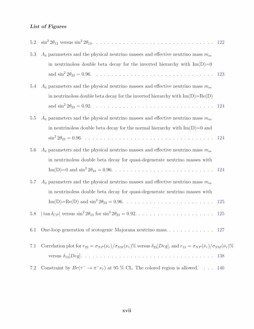
5.2 sin2 2θ12 versus sin2 2θ13. . . . . . . . . . . . . . . . . . . . . . . . . . . . . . . . 122
5.3 A4 parameters and the physical neutrino masses and effective neutrino mass mee
in neutrinoless double beta decay for the inverted hierarchy with Im(D)=0
and sin2 2θ23 = 0.96. . . . . . . . . . . . . . . . . . . . . . . . . . . . . . . . 123
5.4 A4 parameters and the physical neutrino masses and effective neutrino mass mee
in neutrinoless double beta decay for the inverted hierarchy with Im(D)=Re(D)
and sin2 2θ23 = 0.92. . . . . . . . . . . . . . . . . . . . . . . . . . . . . . . . 124
5.5 A4 parameters and the physical neutrino masses and effective neutrino mass mee
in neutrinoless double beta decay for the normal hierarchy with Im(D)=0 and
sin2 2θ23 = 0.96. . . . . . . . . . . . . . . . . . . . . . . . . . . . . . . . . . . 124
5.6 A4 parameters and the physical neutrino masses and effective neutrino mass mee
in neutrinoless double beta decay for quasi-degenerate neutrino masses with
Im(D)=0 and sin2 2θ23 = 0.96. . . . . . . . . . . . . . . . . . . . . . . . . . . 124
5.7 A4 parameters and the physical neutrino masses and effective neutrino mass mee
in neutrinoless double beta decay for quasi-degenerate neutrino masses with
Im(D)=Re(D) and sin2 2θ23 = 0.96. . . . . . . . . . . . . . . . . . . . . . . . 125
5.8 | tan δCP | versus sin2 2θ13 for sin2 2θ23 = 0.92. . . . . . . . . . . . . . . . . . . . . 125
6.1 One-loop generation of scotogenic Majorana neutrino mass. . . . . . . . . . . . . 127
7.1 Correlation plot for r23 = σNP (ντ )/σSM(ντ )% versus δ23[Deg], and r13 = σNP (ντ )/σSM(ντ )%
versus δ13[Deg]. . . . . . . . . . . . . . . . . . . . . . . . . . . . . . . . . . . 138
7.2 Constraint by Br(τ− → π−ντ ) at 95 % CL. The colored region is allowed. . . . 146
xvii
List of Figures
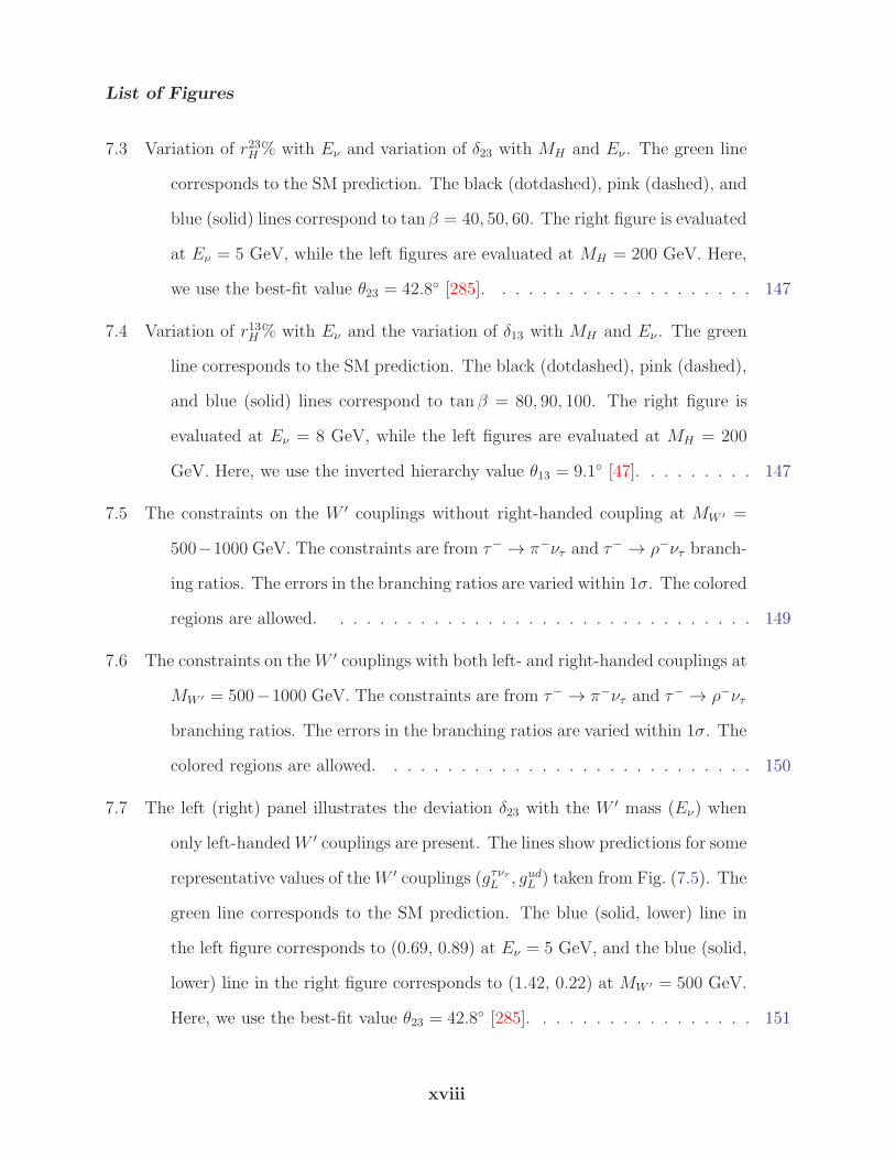
7.3 Variation of r23H% with Eν and variation of δ23 with MH and Eν . The green line
corresponds to the SM prediction. The black (dotdashed), pink (dashed), and
blue (solid) lines correspond to tan β = 40, 50, 60. The right figure is evaluated
at Eν = 5 GeV, while the left figures are evaluated at MH = 200 GeV. Here,
we use the best-fit value θ23 = 42.8 [285]. . . . . . . . . . . . . . . . . . . . 147
7.4 Variation of r13H% with Eν and the variation of δ13 with MH and Eν . The green
line corresponds to the SM prediction. The black (dotdashed), pink (dashed),
and blue (solid) lines correspond to tan β = 80, 90, 100. The right figure is
evaluated at Eν = 8 GeV, while the left figures are evaluated at MH = 200
GeV. Here, we use the inverted hierarchy value θ13 = 9.1 [47]. . . . . . . . . 147
7.5 The constraints on the W ′ couplings without right-handed coupling at MW ′ =
500−1000 GeV. The constraints are from τ− → π−ντ and τ− → ρ−ντ branch-
ing ratios. The errors in the branching ratios are varied within 1σ. The colored
regions are allowed. . . . . . . . . . . . . . . . . . . . . . . . . . . . . . . . 149
7.6 The constraints on theW ′ couplings with both left- and right-handed couplings at
MW ′ = 500−1000 GeV. The constraints are from τ− → π−ντ and τ− → ρ−ντ
branching ratios. The errors in the branching ratios are varied within 1σ. The
colored regions are allowed. . . . . . . . . . . . . . . . . . . . . . . . . . . . 150
7.7 The left (right) panel illustrates the deviation δ23 with the W ′ mass (Eν) when
only left-handedW ′ couplings are present. The lines show predictions for some
representative values of theW ′ couplings (gτντL , gudL ) taken from Fig. (7.5). The
green line corresponds to the SM prediction. The blue (solid, lower) line in
the left figure corresponds to (0.69, 0.89) at Eν = 5 GeV, and the blue (solid,
lower) line in the right figure corresponds to (1.42, 0.22) at MW ′ = 500 GeV.
Here, we use the best-fit value θ23 = 42.8 [285]. . . . . . . . . . . . . . . . . 151
xviii
List of Figures
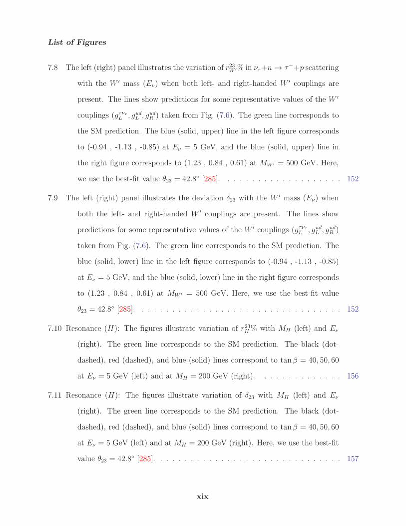
7.8 The left (right) panel illustrates the variation of r23W ′% in ντ+n→ τ−+p scattering
with the W ′ mass (Eν) when both left- and right-handed W ′ couplings are
present. The lines show predictions for some representative values of the W ′
couplings (gτντL , gudL , gudR ) taken from Fig. (7.6). The green line corresponds to
the SM prediction. The blue (solid, upper) line in the left figure corresponds
to (-0.94 , -1.13 , -0.85) at Eν = 5 GeV, and the blue (solid, upper) line in
the right figure corresponds to (1.23 , 0.84 , 0.61) at MW ′ = 500 GeV. Here,
we use the best-fit value θ23 = 42.8 [285]. . . . . . . . . . . . . . . . . . . . 152
7.9 The left (right) panel illustrates the deviation δ23 with the W ′ mass (Eν) when
both the left- and right-handed W ′ couplings are present. The lines show
predictions for some representative values of the W ′ couplings (gτντL , gudL , gudR )
taken from Fig. (7.6). The green line corresponds to the SM prediction. The
blue (solid, lower) line in the left figure corresponds to (-0.94 , -1.13 , -0.85)
at Eν = 5 GeV, and the blue (solid, lower) line in the right figure corresponds
to (1.23 , 0.84 , 0.61) at MW ′ = 500 GeV. Here, we use the best-fit value
θ23 = 42.8 [285]. . . . . . . . . . . . . . . . . . . . . . . . . . . . . . . . . . 152
7.10 Resonance (H): The figures illustrate variation of r23H% with MH (left) and Eν
(right). The green line corresponds to the SM prediction. The black (dot-
dashed), red (dashed), and blue (solid) lines correspond to tanβ = 40, 50, 60
at Eν = 5 GeV (left) and at MH = 200 GeV (right). . . . . . . . . . . . . . 156
7.11 Resonance (H): The figures illustrate variation of δ23 with MH (left) and Eν
(right). The green line corresponds to the SM prediction. The black (dot-
dashed), red (dashed), and blue (solid) lines correspond to tanβ = 40, 50, 60
at Eν = 5 GeV (left) and at MH = 200 GeV (right). Here, we use the best-fit
value θ23 = 42.8 [285]. . . . . . . . . . . . . . . . . . . . . . . . . . . . . . . 157
xix
List of Figures
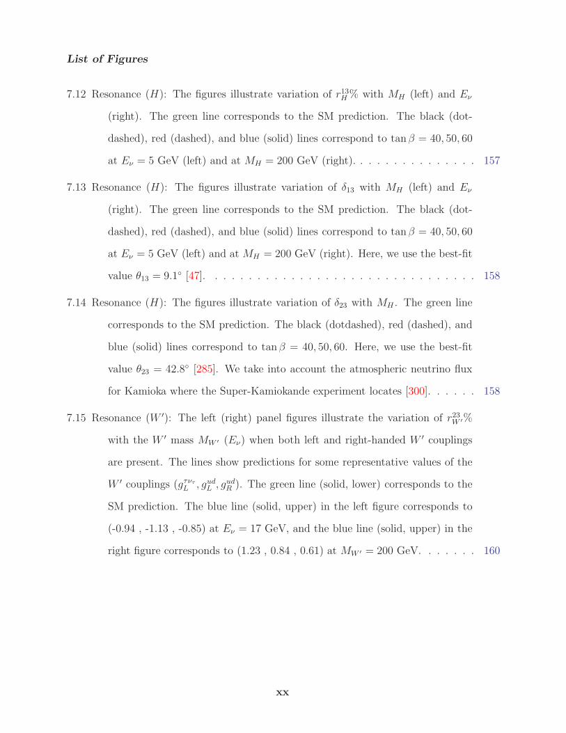
7.12 Resonance (H): The figures illustrate variation of r13H% with MH (left) and Eν
(right). The green line corresponds to the SM prediction. The black (dot-
dashed), red (dashed), and blue (solid) lines correspond to tanβ = 40, 50, 60
at Eν = 5 GeV (left) and at MH = 200 GeV (right). . . . . . . . . . . . . . . 157
7.13 Resonance (H): The figures illustrate variation of δ13 with MH (left) and Eν
(right). The green line corresponds to the SM prediction. The black (dot-
dashed), red (dashed), and blue (solid) lines correspond to tanβ = 40, 50, 60
at Eν = 5 GeV (left) and at MH = 200 GeV (right). Here, we use the best-fit
value θ13 = 9.1 [47]. . . . . . . . . . . . . . . . . . . . . . . . . . . . . . . . 158
7.14 Resonance (H): The figures illustrate variation of δ23 with MH . The green line
corresponds to the SM prediction. The black (dotdashed), red (dashed), and
blue (solid) lines correspond to tanβ = 40, 50, 60. Here, we use the best-fit
value θ23 = 42.8 [285]. We take into account the atmospheric neutrino flux
for Kamioka where the Super-Kamiokande experiment locates [300]. . . . . . 158
7.15 Resonance (W ′): The left (right) panel figures illustrate the variation of r23W ′%
with the W ′ mass MW ′ (Eν) when both left and right-handed W ′ couplings
are present. The lines show predictions for some representative values of the
W ′ couplings (gτντL , gudL , gudR ). The green line (solid, lower) corresponds to the
SM prediction. The blue line (solid, upper) in the left figure corresponds to
(-0.94 , -1.13 , -0.85) at Eν = 17 GeV, and the blue line (solid, upper) in the
right figure corresponds to (1.23 , 0.84 , 0.61) at MW ′ = 200 GeV. . . . . . . 160
xx
List of Figures
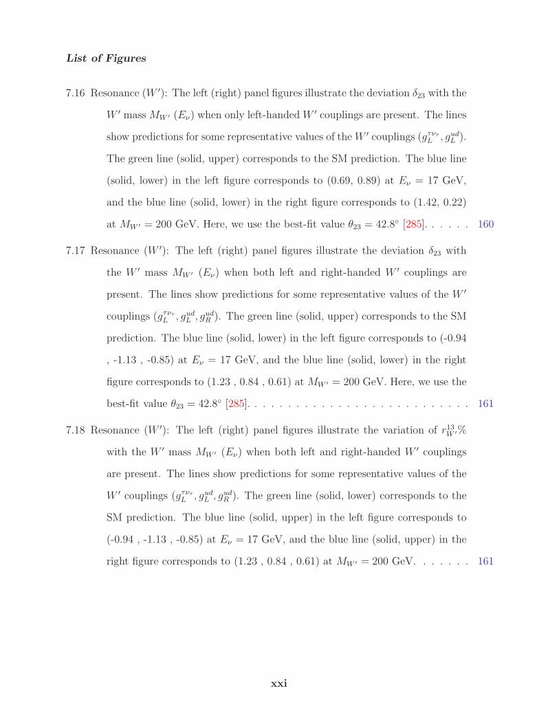
7.16 Resonance (W ′): The left (right) panel figures illustrate the deviation δ23 with the
W ′ massMW ′ (Eν) when only left-handedW ′ couplings are present. The lines
show predictions for some representative values of theW ′ couplings (gτντL , gudL ).
The green line (solid, upper) corresponds to the SM prediction. The blue line
(solid, lower) in the left figure corresponds to (0.69, 0.89) at Eν = 17 GeV,
and the blue line (solid, lower) in the right figure corresponds to (1.42, 0.22)
at MW ′ = 200 GeV. Here, we use the best-fit value θ23 = 42.8 [285]. . . . . . 160
7.17 Resonance (W ′): The left (right) panel figures illustrate the deviation δ23 with
the W ′ mass MW ′ (Eν) when both left and right-handed W ′ couplings are
present. The lines show predictions for some representative values of the W ′
couplings (gτντL , gudL , gudR ). The green line (solid, upper) corresponds to the SM
prediction. The blue line (solid, lower) in the left figure corresponds to (-0.94
, -1.13 , -0.85) at Eν = 17 GeV, and the blue line (solid, lower) in the right
figure corresponds to (1.23 , 0.84 , 0.61) at MW ′ = 200 GeV. Here, we use the
best-fit value θ23 = 42.8 [285]. . . . . . . . . . . . . . . . . . . . . . . . . . . 161
7.18 Resonance (W ′): The left (right) panel figures illustrate the variation of r13W ′%
with the W ′ mass MW ′ (Eν) when both left and right-handed W ′ couplings
are present. The lines show predictions for some representative values of the
W ′ couplings (gτντL , gudL , gudR ). The green line (solid, lower) corresponds to the
SM prediction. The blue line (solid, upper) in the left figure corresponds to
(-0.94 , -1.13 , -0.85) at Eν = 17 GeV, and the blue line (solid, upper) in the
right figure corresponds to (1.23 , 0.84 , 0.61) at MW ′ = 200 GeV. . . . . . . 161
xxi
List of Figures
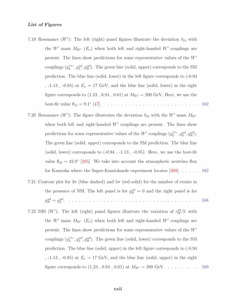
7.19 Resonance (W ′): The left (right) panel figures illustrate the deviation δ13 with
the W ′ mass MW ′ (Eν) when both left and right-handed W ′ couplings are
present. The lines show predictions for some representative values of the W ′
couplings (gτντL , gudL , gudR ). The green line (solid, upper) corresponds to the SM
prediction. The blue line (solid, lower) in the left figure corresponds to (-0.94
, -1.13 , -0.85) at Eν = 17 GeV, and the blue line (solid, lower) in the right
figure corresponds to (1.23 , 0.84 , 0.61) at MW ′ = 200 GeV. Here, we use the
best-fit value θ13 = 9.1 [47]. . . . . . . . . . . . . . . . . . . . . . . . . . . 162
7.20 Resonance (W ′): The figure illustrates the deviation δ23 with the W ′ mass MW ′
when both left and right-handed W ′ couplings are present. The lines show
predictions for some representative values of the W ′ couplings (gτντL , gudL , gudR ).
The green line (solid, upper) corresponds to the SM prediction. The blue line
(solid, lower) corresponds to (-0.94 , -1.13 , -0.85). Here, we use the best-fit
value θ23 = 42.8 [285]. We take into account the atmospheric neutrino flux
for Kamioka where the Super-Kamiokande experiment locates [300]. . . . . . 162
7.21 Contour plot for 3σ (blue dashed) and 5σ (red solid) for the number of events in
the presence of NSI. The left panel is for gudR = 0 and the right panel is for
gudR = gudL . . . . . . . . . . . . . . . . . . . . . . . . . . . . . . . . . . . . . . 168
7.22 DIS (W ′): The left (right) panel figures illustrate the variation of r23W ′% with
the W ′ mass MW ′ (Eν) when both left and right-handed W ′ couplings are
present. The lines show predictions for some representative values of the W ′
couplings (gτντL , gudL , gudR ). The green line (solid, lower) corresponds to the SM
prediction. The blue line (solid, upper) in the left figure corresponds to (-0.94
, -1.13 , -0.85) at Eν = 17 GeV, and the blue line (solid, upper) in the right
figure corresponds to (1.23 , 0.84 , 0.61) at MW ′ = 200 GeV. . . . . . . . . . 169
xxii
List of Figures
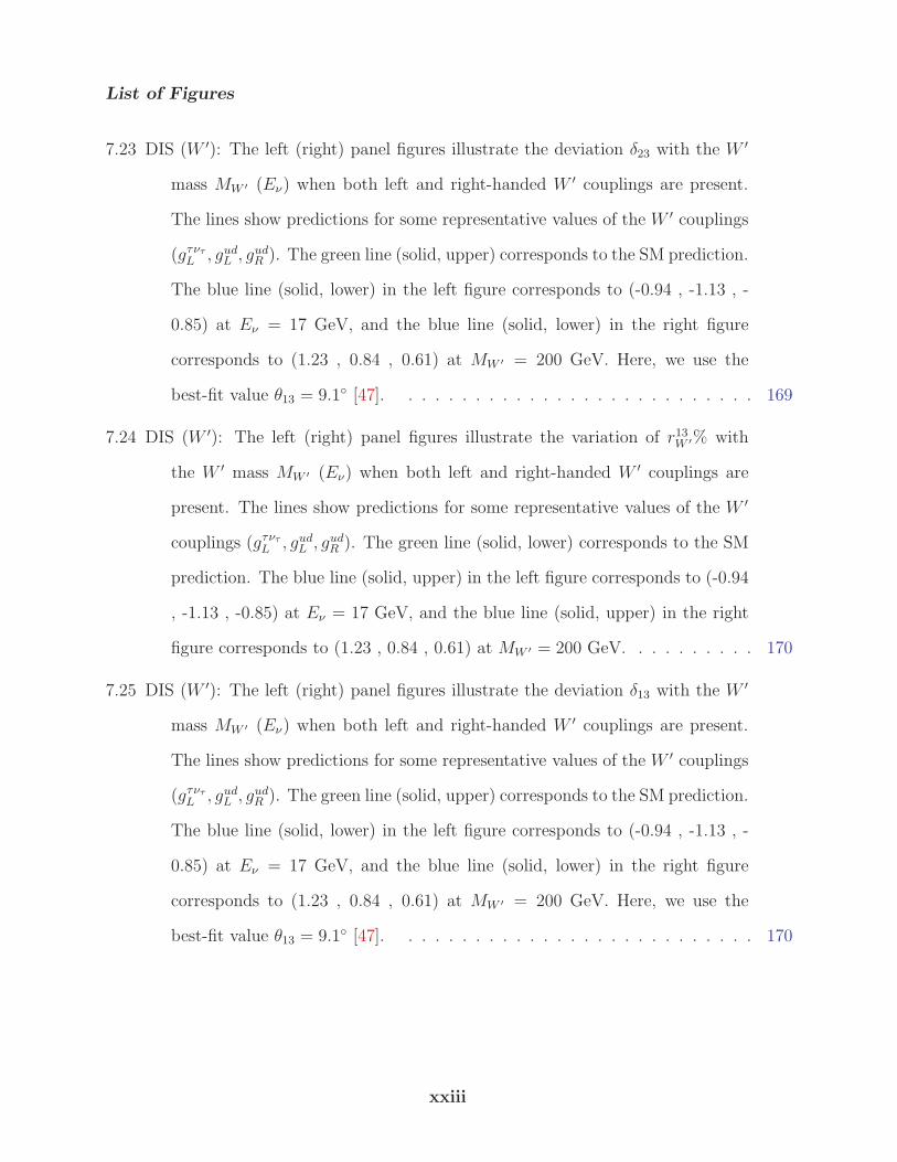
7.23 DIS (W ′): The left (right) panel figures illustrate the deviation δ23 with the W ′
mass MW ′ (Eν) when both left and right-handed W ′ couplings are present.
The lines show predictions for some representative values of the W ′ couplings
(gτντL , gudL , gudR ). The green line (solid, upper) corresponds to the SM prediction.
The blue line (solid, lower) in the left figure corresponds to (-0.94 , -1.13 , -
0.85) at Eν = 17 GeV, and the blue line (solid, lower) in the right figure
corresponds to (1.23 , 0.84 , 0.61) at MW ′ = 200 GeV. Here, we use the
best-fit value θ13 = 9.1 [47]. . . . . . . . . . . . . . . . . . . . . . . . . . . 169
7.24 DIS (W ′): The left (right) panel figures illustrate the variation of r13W ′% with
the W ′ mass MW ′ (Eν) when both left and right-handed W ′ couplings are
present. The lines show predictions for some representative values of the W ′
couplings (gτντL , gudL , gudR ). The green line (solid, lower) corresponds to the SM
prediction. The blue line (solid, upper) in the left figure corresponds to (-0.94
, -1.13 , -0.85) at Eν = 17 GeV, and the blue line (solid, upper) in the right
figure corresponds to (1.23 , 0.84 , 0.61) at MW ′ = 200 GeV. . . . . . . . . . 170
7.25 DIS (W ′): The left (right) panel figures illustrate the deviation δ13 with the W ′
mass MW ′ (Eν) when both left and right-handed W ′ couplings are present.
The lines show predictions for some representative values of the W ′ couplings
(gτντL , gudL , gudR ). The green line (solid, upper) corresponds to the SM prediction.
The blue line (solid, lower) in the left figure corresponds to (-0.94 , -1.13 , -
0.85) at Eν = 17 GeV, and the blue line (solid, lower) in the right figure
corresponds to (1.23 , 0.84 , 0.61) at MW ′ = 200 GeV. Here, we use the
best-fit value θ13 = 9.1 [47]. . . . . . . . . . . . . . . . . . . . . . . . . . . 170
xxiii
List of Figures
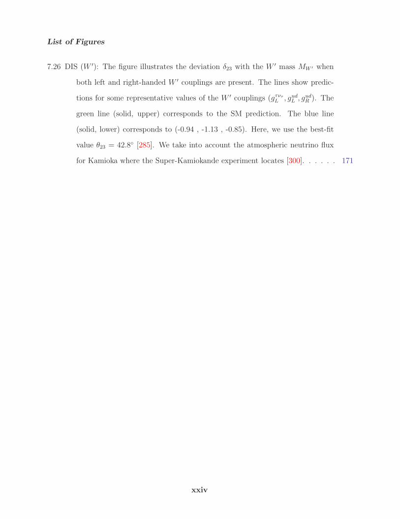
7.26 DIS (W ′): The figure illustrates the deviation δ23 with the W ′ mass MW ′ when
both left and right-handed W ′ couplings are present. The lines show predic-
tions for some representative values of the W ′ couplings (gτντL , gudL , gudR ). The
green line (solid, upper) corresponds to the SM prediction. The blue line
(solid, lower) corresponds to (-0.94 , -1.13 , -0.85). Here, we use the best-fit
value θ23 = 42.8 [285]. We take into account the atmospheric neutrino flux
for Kamioka where the Super-Kamiokande experiment locates [300]. . . . . . 171
xxiv
Chapter 1
Introduction
The standard model (SM) of particle physics is a SU(3) × SU(2) × U(1) gauge theory
which combines the color gauge group SU(3) of the strong interaction with the Glashow-
Weinberg-Salam (GWS) model of electroweak theory (SU(2)× U(1)). The standard model
recognizes two types of elementary fermions: quarks and leptons. The model distinguishes
twelve different fermions: six quarks and six leptons, each with a corresponding anti-particle.
Each quark comes in three different color charges, while the remaining fermions (leptons)
do not carry color charge. They are arranged in a very tidy symmetrical structure. They
are arranged under SU(2) in six left-handed families: three families consist of two quarks
forming doublets, and another three consist of two leptons each. Each left-handed fermion
has a corresponding right-handed one that does not contribute in the doublets. Quarks and
leptons are the building blocks which build up matter, i.e., they are seen as the “elementary
particles”. In the standard model, gauge bosons are defined as force carriers that mediate
the strong, weak, and electromagnetic fundamental interactions. The strong interaction is
mediated by massless vector boson so-called gluon, of which there are eight. The weak inter-
action has two massive charged mediators (W±) and one neutral (Z0). The electromagnetic
interaction couples to all charged quarks and leptons via the photon. Lastly, the Higgs bo-
son is the only scalar particle that exists in the SM. In 2012 a previously unknown boson
was discovered at the Large Hadron Collider (LHC); its properties are still being studied to
confirm whether or not it is the Higgs boson.
Quarks are peculiar as they posses electric charges which are fractions of that for the
electron. A phenomenon called color confinement results in quarks being perpetually bound
to one another, forming color-neutral composite particles called hadrons. There are two
1
types of hadrons, the Baryon which is a system of three quarks (e.g. the proton) or Mesons,
a two quark system containing a quark - antiquark pair (e.g. the pion or pi-meson). For
leptons, electron, muon and tau (which are referred to as different flavors of the lepton),
there is a corresponding neutrino associated with it. Leptons do not participate in the
strong interaction and are generally not seen within the nucleus. The discovery of neutrino
mass via flavor oscillations is a clear sign of physics beyond the standard model (BSM).
Originally, the evidence of this phenomenon was of astrophysical origin but now it has been
convincingly confirmed by terrestrial experiments.
Despite the spectacular achievements in the last ten years or so, a lot of open questions
are still seeking for answers to complete our understanding of the neutrino sector. In the
following, we mention some of them:
• What is the sign of the mass squared difference ∆m231(≡ m2
3 −m21) or the character of
the neutrino mass hierarchy?
• What is the mass scale of the neutrinos? Why are neutrino masses so small?
• Why is the pattern of the neutrino mixing so different from that of the quarks? Is
there any connection between quarks and leptons?
• Are the neutrinos Dirac or Majorana particles?
• Is sin2 2θ23, where θ23 is the atmospheric mixing angle, exactly maximal (= 1)? If
sin2 2θ23 6= 1, what is its octant?
• How many neutrino species are there? Do sterile neutrinos exist? Are three-flavor
oscillations enough?
non-zero value for θ13 has been observed by MINOS and T2K experiments [1, 2, 3]
would increase the possibility of observing CP-violation in the lepton sector. Non-zero θ13
also brings in the possibility of large Earth matter effects [4] for GeV energy accelerator
2
1.1 Higgs in the Standard Model and multi-Higgs-doublet models
neutrinos travelling over long distances. Matter effect on neutrino oscillations depends on
the sgn(∆m231).It is opposite for neutrinos and anti-neutrinos. For a given sgn(∆m2
31) it
enhances the oscillation probability in one of the channels and suppresses it in the other.
Thus, comparing the neutrino signal against the anti-neutrino signal in very long baseline
experiments gives a powerful tool to determine sgn(∆m231).
In this dissertation we study the effects of multi-Higgs doublets on the properties of
the neutrino sector and heavy quark systems. The dissertation is organised as follows: In
the rest of the introduction we present a general background of two-Higgs-doublet model
(2HDM), heavy quark systems, top forward-backward asymmetry, and neutrino sector. In
the following chapters we discuss the phenomenological implications of the 2HDM in neutrino
mixing models, non-standard neutrino interactions, and heavy quarkonium system, as well
as in the study of the top forward-backward asymmetry.
1.1 Higgs in the Standard Model and multi-Higgs-doublet
models
The Higgs mechanism is a simple method for explaining the electroweak symmetry breaking
and developing masses for the electroweak gauge bosons, the W± and the Z0, as well as all
elementary fermions; leptons and quarks. It was first proposed in 1964 by Higgs, Kibble,
Guralnik, Hagen, Englert and Brout [5, 6, 7]. The Higgs mechanism has become the corner
stone of the standard model for explaining the origin of the particle masses. In the SM, one
complex doublet of scalar fields with a non trivial potential is introduced as
Φ =
φ+
φ0
=
φ1 + iφ2
φ3 + iφ4
(1.1)
3
1.1 Higgs in the Standard Model and multi-Higgs-doublet models
to provide masses to both the weak force carriers and the elementary matter particles. The
Higgs doublet transforms as an SU (2)L doublet, and its weak hypercharge is Y = 1. The
price of proposing the Higgs mechanism is the presence of just one new massive Higgs particle
or Higgs boson.
The Higgs Lagrangian consists of three terms: the scalar potential, the kinetic term, and
the Yukawa terms
V (Φ+Φ) = µ2(Φ+Φ) + λ(Φ+Φ)2,
£kin = (DµΦ) (DµΦ)† ; Dµ ≡ ∂µ −
ig′
2YW 4
µ − igτiWiµ,
−£Y = ηUijQLΦUR + ηDijQLΦDR + ηℓijℓLΦER + h.c. (1.2)
where µ2 and λ are free parameters of the theory. W iµ with i = 1, 2, 3 are the four-vector
fields (gauge eigenstates), associated with the three generators τi of SU (2)L symmetry.
On the other hand, W 4µ is the four-vector field associated to the Y generator i.e. the
U (1)Y symmetry. g and g′ are the coupling strengths associated with W iµ and W 4
µ , respec-
tively. QL is the left-handed quark doublet, UR, DR are the right-handed singlets of the up
and down sectors of quarks. ℓL is the left-handed lepton doublet, ER is the right-handed
singlet of the down sector of leptons. The Yukawa couplings ηU,D,ℓij define the vertices and,
consequently, the Feynman rules of the Lagrangian where i, j are family indices. The sponta-
neous symmetry breaking describes systems where the Lagrangian obeys certain symmetries,
but the lowest energy solutions do not exhibit that symmetry. The Higgs potential generates
the spontaneous symmetry breaking when µ2 < 0 . The above potential is the most general
renormalizable potential invariant under the SM symmetry group SU (2)L×U (1)Y . The ki-
netic term describes the interactions between scalar particles and vector bosons, and provides
the masses for the latter when the Higgs field acquires a vacuum expectation value (VEV).
The Yukawa Lagrangian describes the interaction among the Higgs bosons and fermions.
4
1.1 Higgs in the Standard Model and multi-Higgs-doublet models
Even though the standard model offers a very successful description of strong and elec-
troweak interactions, it fails in providing an explanation for issues such as the gauge group,
the number of families, the dynamics of flavor and the mechanism of mass generation, among
others. This suggests the SM is not a fundamental theory but a part of a more complete
theory. There are many extensions of the SM have been proposed. Several such models, like
supersymmetry, contain an extended Higgs sector. The simplest extended Higgs sector is a
two Higgs doublet model (2HDM) which constitutes of two, instead of one, complex scalar
doublets as
Φ1 =
φ+1
φ01
, Φ2 =
φ+2
φ02
, (1.3)
with hypercharges (Y1 = Y2 = 1). In the so-called 2HDM-II model Φ1 couples to the up-type
and Φ2 to the down-type quarks respectively. Upon spontaneous symmetry breaking, the
neutral components of Φ1 and Φ2 acquire vacuum expectation values
〈Φ1〉 =v1√2, 〈Φ2〉 =
v2√2eiξ. (1.4)
So it is more convenient to parametrize the doublets in the following way
Φ1 =
φ+1
h1+v1+ig1√2
; Φ2 =
φ+2
h2+v2+ig2√2
(1.5)
where ξ is a phase parameter and
g1 =√2Im(φ0
1), g2 =√2Im(φ0
2),
h1 =√2(Re(φ0
1)− v1), h2 =
√2(Re(φ0
2)− v2). (1.6)
The mass eigenstastes are obtained from the gauge eigenstates defined in (1.5) by the
following transformations
5
1.1 Higgs in the Standard Model and multi-Higgs-doublet models
cos β sin β
− sin β cos β
φ±1
φ±2
=
G±
H±
,
cosα sinα
− sinα cosα
h1
h2
=
H0
h0
,
cos β sin β
− sin β cos β
g1
g2
=
G0
A0
. (1.7)
Only three of the eight original scalar degrees of freedom (corresponding to two complex dou-
blet) are reabsorbed in transforming the originally massless vector bosons into massive ones,
i.e. three Goldstone bosons (G±, G0) corresponding to W±, Z, respectively. The remaining
five degrees of freedom correspond to physical degrees of freedom in the form of: two neutral
CP-even scalars (H0, h0), one neutral pseudoscalar (CP-odd) A0, and two charged scalar
fields (H±). A key parameter of the model is the ratio of the vacuum expectation values
tanβ =v2v1. (1.8)
The Higgs potential which spontaneously breaks SU(2)L ×U(1)Y down to U(1)EM is [8]
V2HD(Φ1, Φ2) = λ1(Φ†1Φ1 − v21)
2 + λ2(Φ†2Φ2 − v22)
2
+ λ3
[(Φ†
1Φ1 − v21) + (Φ†2Φ2 − v22)
]2
+ λ4
[(Φ†
1Φ1)(Φ†2Φ2)− (Φ†
1Φ2)(Φ†2Φ1)
]
+ λ5
[Re(Φ†
1Φ2)− v1v2 cos ξ]2
+ λ6
[Im(Φ†
1Φ2)− v1v2 sin ξ]2, (1.9)
where λi are real parameters (by hermiticity). The kinetic Lagrangian and the most general
6
1.1 Higgs in the Standard Model and multi-Higgs-doublet models
gauge invariant Lagrangian that couples the Higgs fields to fermions read
£kin = (DµΦ1)+(DµΦ1) + (DµΦ2)
+(DµΦ2),
−£Y = ηU,0ij Q0
iLΦ1U0jR + ηD,0
ij Q0
iLΦ1D0jR + ξU,0ij Q
0
iLΦ2U0jR + ξD,0
ij Q0
iLΦ2D0jR +
ηE,0ij l
0
iLΦ1E0jR + ξE,0
ij l0
iLΦ2E0jR + h.c., (1.10)
where Φ1,2 ≡ iσ2Φ1,2, η0ij and ξ
0ij are non diagonal 3×3 matrices and i, j denote family indices.
D0R refers to the three down-type weak isospin quark singlets D0
R ≡ (d0R, s0R, b
0R)
T, U refers
to the three up-type weak isospin quark singlets U0R ≡ (u0R, c
0R, t
0R)
Tand E0
R to the three
charged leptons. Finally, Q0
iL, l0
iL denote the quark and lepton weak isospin left-handed
doublets respectively. The superscript “0” indicates that the fields are not mass eigenstates
yet.
The real CP-even sector contains two physical Higgs scalars (H0, h0) which mix through
the following mass-squared matrix
M =
4v21(λ1 + λ3) + v22λ5 (4λ3 + λ5)v1v2
(4λ3 + λ5)v1v2 4v22(λ2 + λ3) + v21λ5
. (1.11)
At tree level, the masses of the scalar and pseudoscalar degrees of freedom satisfy the fol-
lowing relations:
M2H± = λ4(v
21 + v22),
M2A0 = λ6(v
21 + v22),
M2H0,h0 =
1
2
(M11 +M22 ±
√(M11 −M22)2 + 4M2
12
), (1.12)
7
1.2 Heavy quarkonium decay
and the mixing angle α is obtained as
sin 2α =2M12√
(M11 −M22)2 + 4M212
,
cos 2α =M11 −M22√
(M11 −M22)2 + 4M212
. (1.13)
1.2 Heavy quarkonium decay
On 4 July 2012 both of the CERN experiments CMS and ATLAS announced they had
independently made the same discovery of new boson state with mass 125.3 ± 0.6 GeV in
CMS [9] and 126.5 GeV in ATLAS [10]. Using the combined analysis, both experiments
reached a local significance of 5σ significance. After the discovery of the boson state, it
is widely anticipated that physics beyond the standard model or new physics (NP) will be
discovered soon at experiments such as the LHC. This NP might contain additional Higgs
bosons beyond the SM Higgs, new gauge bosons, or new quarks and leptons. It is generally
believed that these new particles will be heavy with masses from the weak scale ∼ 100 GeV
to a TeV. However, light scalars and vector bosons with masses in the GeV range or even
lower are not ruled out. For instance, light scalar states coming from a primary higgs with
non SM decays can be consistent with existing experimental constraints [11]. One of the
ways to probe these light states is to look at decays of particles with masses in the 10 GeV
range such as the Υ. Data from the present and future B factories can be used to search for
these states and/or to put constraints on models that predict such states.
It is also possible to probe these light states via the ηb decays. The pseudoscalar bb bound
state in the 1S configuration, the ηb, was observed in BaBar by two different experiments.
First, it was seen in the decay of Υ(3S) → γηb [12] with a signal significance greater than
10 standard deviations (σ). The ηb was observed in the photon energy spectrum using
(109± 1) million Υ(3S) events and the hyperfine Υ(1S)− ηb mass splitting was measured to
8
1.3 Forward-backward asymmetry in top physics
be 71.4+2.3−3.1(stat)± 2.7(syst) MeV from the mass m(ηb) = 9388.9+3.1
−2.3 (stat)± 2.7 (syst) MeV.
Soon after, it was also seen in Υ(2S) → γηb [13] by another group in BaBar, and the
hyperfine mass splitting was determined to be 67.4+4.8−4.6(stat)± 2.0(syst) MeV from the mass
m(ηb) = 9392.9+4.6−4.8 (stat) ± 1.9 (syst) MeV. In the past, since the discovery of the Υ(nS)
resonances [14] in 1977, various experimental environments [15, 16, 17] have been used to
seek the ground state ηb but without success. Many theoretical models have attempted
to predict the mass of ηb. Lattice NRQCD [18, 19] predicts the hyperfine splitting to be
Elathfs = 61 ± 14 MeV and correspondingly the mass to be mηb = 9383(4)(2) MeV which is
in agreement with the experimental results. The calculations of perturbative QCD based
models [19, 20] predict the hyperfine splitting to be EQCDhfs = 39±11(th)+9
−8(δαs) MeV which is
smaller than the measured values. Experiments at BaBar have also searched for a low-mass
Higgs boson in Υ(3S) → γA0, A0 → τ+τ− [21] with data sample containing 122 million
Υ(3S) events. In the same analysis, constraint on the branching ratio for ηb → τ+τ− was
reported as BR(ηb → τ+τ−) < 8% at 90% confidence level (C.L.).
Here we explore the decay ηb → τ+τ− as a probe for a light pseudoscalar or a light axial
vector state. We estimate the standard model branching ratio for this decay to be ∼ 4×10⁻⁹.
We show that considerably larger branching ratios, up to the present experimental limit of
∼ 8%, is possible in models with a light pseudoscalar or a light axial vector state.
1.3 Forward-backward asymmetry in top physics
The top quark with its high mass may play a crucial role in electroweak symmetry breaking.
Hence the top sector may be sensitive to new physics effects that could be revealed through
careful measurements of top quark properties. The top quark pair production in proton-
antiproton collisions at the Tevatron collider with a center-of-mass (CM) energy of√s = 1.96
TeV is dominated by the partonic process qq → tt. Recently the CDF experiment has
9
1.4 Neutrino oscillation
reported a measurement of forward-backward asymmetry in tt production which appears
to deviate from the standard model predictions. The CDF collaboration measured the
forward-backward asymmetry (AFB) in top quark pair production in the tt rest frame to
be AttFB = 0.475 ± 0.774 for Mtt > 450 GeV [22], which is 3.4 σ deviations from the next-
to leading order (NLO) SM prediction AttFB = 0.088 ± 0.013 [23, 24, 25, 26]. The DØ
collaboration also observed a larger than predicted asymmetry [27].
The current measurement of the top quark pair production cross section from 4.6 fb−1 of
data at CDF is
σtt = (7.50± 0.48)pb , (1.14)
for mt = 172.5 GeV [28], in good agreement with their SM predictions by Langenfeld et
al. σtt = 7.46+0.66−0.80 pb [29], Cacciari et al. σtt = 7.26+0.78
−0.86 pb [30], Kidonakis σtt = 7.29+0.79−0.85
pb [31], and recent Ahrens et al.’s significantly low value σtt = 6.30 ± 0.190.31−0.23 pb [32].
Hence new physics models that aim to explain the AFB measurement must not change the
production cross section appreciably. Many NP models that affect AFB, either via s-channel
[33] or t-channel exchange of new particles [34] have been proposed to explain the forward-
backward anomaly. Here we will study the forward-backward asymmetry measurement in
the presence of Z ′ boson contribution. We consider a flavor-changing tuZ ′ coupling which
can contribute to tt production in the t-channel including tensor term in the coupling, and
study the effects on the top AFB.
1.4 Neutrino oscillation
Neutrino oscillation is a quantum mechanical phenomenon of lepton flavor changing for a
neutrino with energy E travelling some distance L between the source and detector. Neutrino
10
1.4 Neutrino oscillation
oscillation has been observed in various experiments. This phenomenon is not expected in
the standard model because neutrinos are massless in this theory and it is always possible
to choose a physical basis where the leptonic Yukawa couplings are diagonal. Neutrino mass
is the most potent evidence of existing physics beyond the standard model.
1.4.1 Current experimental situation
The first experimental observation of the electron neutrino was in 1956 in the nuclear fission
products in the nuclear reactor beta decay. Neutrino was first postulated in 1930 by Wolf-
gang Pauli in order to preserve the conservation of energy, conservation of momentum, and
conservation of angular momentum (spin) in β-decay n→ p+ e−+ νe. Soon later, the muon
neutrino νµ was discovered. It was assumed to be the same neutrino that was discovered in
the beta decay till Schwarz, Steinberger and Lederman performed a neutrino experiment to
prove the existence of two kinds of neutrinos through the pion decay π+ → µ+ + νµ.
The conception of the standard model, established in the mid 1970s, postulated that the
fermions, consisting of the electron, muon, tau and the neutrinos, form a doublet structure
such that the electron is grouped with νe, the muon is grouped with νµ and the tau is grouped
with ντ . The third type of neutrino, ντ was observed in 2000 by the DONUT collaboration
[35]. The experiment used a neutrino beam created by Ds → τ ντ and the decay of τ into
another ντ .
The last decades have been extremely successful for the field of neutrino physics. It
was not until 1998 that the existence of neutrino oscillations was finally established experi-
mentally by the Super-Kamiokande experiment in Japan for atmospheric neutrinos [36]. In
2002, the SNO collaboration demonstrated that the solar neutrino problem i.e. the major
discrepancy between measurements of the numbers of neutrinos flowing through the Earth
and theoretical models of the solar interior [37] is solved by solar neutrino oscillations [38].
11
1.4 Neutrino oscillation
parameter best fit 1σ range 2σ range 3σ range∆m2
21 · · · [10−5eV2] 7.62 7.43–7.81 7.27–8.01 7.12–8.20
|∆m231| · · · [10−3eV2]
2.552.43
2.46− 2.612.37− 2.50
2.38− 2.682.29− 2.58
2.31− 2.742.21− 2.64
sin2 θ12 0.320 0.303–0.336 0.29–0.35 0.27–0.37
sin2 θ230.613 (0.427)1
0.600
0.400-0.461(0.573–0.635)0.569–0.626
0.38–0.660.39–0.65
0.36–0.680.37–0.67
sin2 θ130.02460.0250
0.0218–0.02750.0223–0.0276
0.019–0.0300.020–0.030
0.017–0.033
δ0.80π
−0.03π0− 2π 0− 2π 0− 2π
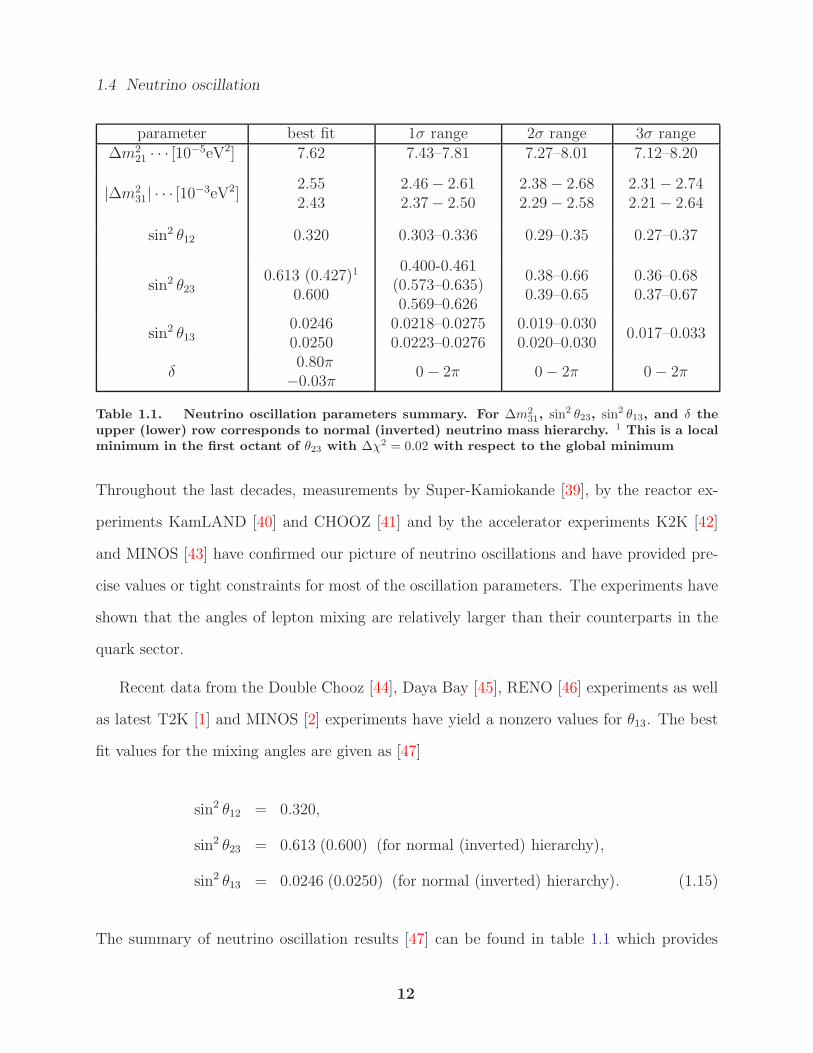
Table 1.1. Neutrino oscillation parameters summary. For ∆m231, sin2 θ23, sin2 θ13, and δ the
upper (lower) row corresponds to normal (inverted) neutrino mass hierarchy. 1 This is a localminimum in the first octant of θ23 with ∆χ2 = 0.02 with respect to the global minimum
Throughout the last decades, measurements by Super-Kamiokande [39], by the reactor ex-
periments KamLAND [40] and CHOOZ [41] and by the accelerator experiments K2K [42]
and MINOS [43] have confirmed our picture of neutrino oscillations and have provided pre-
cise values or tight constraints for most of the oscillation parameters. The experiments have
shown that the angles of lepton mixing are relatively larger than their counterparts in the
quark sector.
Recent data from the Double Chooz [44], Daya Bay [45], RENO [46] experiments as well
as latest T2K [1] and MINOS [2] experiments have yield a nonzero values for θ13. The best
fit values for the mixing angles are given as [47]
sin2 θ12 = 0.320,
sin2 θ23 = 0.613 (0.600) (for normal (inverted) hierarchy),
sin2 θ13 = 0.0246 (0.0250) (for normal (inverted) hierarchy). (1.15)
The summary of neutrino oscillation results [47] can be found in table 1.1 which provides
12
1.4 Neutrino oscillation
best fit points, 1σ errors, and the allowed intervals at 2 and 3σ for the three-flavor oscillation
parameters. There are several papers that have attempted to explain the recent θ13 results
[48, 49].
Neutrino oscillation experiments are only sensitive to mass squared differences. Thus,
they cannot provide information on the absolute neutrino masses. However, kinematical
studies of the electron spectrum in nuclear β-decay [50] produce upper limit to the absolute
neutrino masses ≤ 2.3 eV (95% C.L.). Also, cosmological observations constrain the absolute
masses to lie below ∼ 0.2 eV [51]. On the other hand, the neutrinoless double beta decay
experiments [52] put a bound at the level of 0.35 eV (90% C.L.) in the case of neutrinos with
Majorana mass terms.
Several experiments have searched for new effects beyond the framework of three massive
neutrinos with standard model interactions. Till now, no evidence for such effects has been
found yet. Instead, constraints have been derived on non-standard neutrino interactions
[53], neutrino decay [54], neutrino decoherence [55], oscillations into sterile neutrinos (i.e.
neutrinos not coupling to the Z boson) [56] and other exotic scenarios.
1.4.2 Mixing and oscillation parameters
There are two different bases of the neutrino field, flavor basis να(α = e, µ, τ) which associate
with the charged lepton partners in the charged weak interactions and has no definite mass
as the mass matrix of neutrinos are non-diagonal, and the mass basis νi(i = 1, 2, 3) which
have definite masses and are the eigenstates of the free Hamiltonian. The fact of lepton
mixing has been firmly established through a variety of solar, atmospheric, and terrestrial
neutrino oscillation experiments [57]. The charged current interaction can be written in the
flavor basis as
− g√2lαγ
µ(1− γ5)ναWµ. (1.16)
13
1.4 Neutrino oscillation
If the charged lepton and neutrino Yukawa matrices are non-diagonal, using the transfor-
mation between the flavor and mass fields the charged current interaction can be written
as
− g√2liγ
µ(1− γ5)UαiνiWµ. (1.17)
If the charged lepton Yukawa matrix is diagonal, the charged current interaction can be
given as
− g√2lαγ
µ(1− γ5)UαiνiWµ, (1.18)
where the mixing between the two bases of the neutrino field can be described by the rela-
tionship
|να〉 =n∑
i=1
Uαi|νi〉, (1.19)
where U is the unitary leptonic mixing matrix. The well known parametrization of the
neutrino mixing matrix is known as Pontecorvo-Maki-Nakagawa-Sakata (PMNS) matrix,
UPMNS [58]:
UPMNS =
c12c13 s12c13 s13e−iδ
−s12c23 − c12s23s13eiδ c12c23 − s12s23s13e
iδ s23c13
s12s23 − c12c23s13eiδ −c12s23 − s12c23s13e
iδ c23c13
K, (1.20)
where s13 ≡ sin θ13, c13 ≡ cos θ13 with θ13 being the reactor angle, s12 ≡ sin θ12, c12 ≡ cos θ12
with θ12 being the solar angle, s23 ≡ sin θ23, c23 ≡ cos θ23 with θ23 being the atmospheric
angle, δ is the Dirac CP violating phase, and K = diag(1, eiφ1, eiφ2) contains additional
(Majorana) CP violating phases φ1, φ2, which are physically relevant if neutrinos are Ma-
jorana particles. Experiments have put no constraints on the Majorana phases, therefore,
we usually ignore them. The experiments have shown that the angles of lepton mixing are
relatively larger than their counterparts in the quark sector.
In order to calculate the probability of flavor changing we need to consider the evaluation
14
1.4 Neutrino oscillation
of the eigenstates in time [59]. Suppose a given source is producing a neutrino flux of given
flavor |να〉 at zero time and zero position t = 0 = x then the neutrino state at a later time t
will be given by
|να(t)〉 =n∑
i=1
U∗αi|νi(t)〉 =
n∑
i=1
U∗αie
−iEit|νi(0)〉, (1.21)
where Ei are the energy eigenvalues associated with the individual neutrino mass eigenstates
νi. The oscillation probability Pαβ for the flavor transition α → β is given by
Pαβ(t) = |〈νβ|να(t)〉|2
=
n∑
i=1
m∑
j=1
J ijαβe
−i(Ei−Ej)t, (1.22)
where the Jarlskog CP-odd invariant J ijαβ is written as
J ijαβ ≡ UβiU
∗αiU
∗βjUαj . (1.23)
For ultra relativistic neutrinos with small mass one can assume pi ≡ p ≃ E and we have
Ei =√p2i +m2
i ≃ p+m2
i
2p= E +
m2i
2E, (1.24)
or
Ei − Ej =∆m2
ji
2E, (1.25)
where ∆m2ji = m2
i − m2j . Let us suppose that t is the travel time of the ultra relativistic
neutrinos from the source to the detector with L is the distance traveled. In the natural
unit, c = 1, we can consider that t ∼= L, thus
(Ei −Ej)t =∆m2
jiL
2E. (1.26)
15
1.4 Neutrino oscillation
Now, the transition probability can be written as
Pαβ =∑
i,j
UβiU∗αiU
∗βjUαje
−i∆m2
jiL
2E
=∑
i
|Uαi|2|Uβi|2 + 2Re∑
i>j
(UβiU
∗αiU
∗βjUαj
)e−i
∆m2jiL
2E . (1.27)
From the orthogonality relation 〈νj |νi〉 = δij one can obtain the following relation
∑
i
|Uαi|2|Uβi|2 = δαβ − 2Re∑
i>j
(UβiU
∗αiU
∗βjUαj
), (1.28)
then
Pαβ = δαβ − 2Re∑
i>j
(UβiU
∗αiU
∗βjUαj
)+ 2Re
∑
i>j
(UβiU
∗αiU
∗βjUαj
)e−i
∆m2jiL
2E
= δαβ − 2Re∑
i>j
(UβiU
∗αiU
∗βjUαj
)(1− e−i
∆m2jiL
2E ). (1.29)
Since for any complex numbers a and b, Re(ab)=Re(a)Re(b)-Im(a)Im(b), then
Pαβ = δαβ − 2Re∑
i>j
(UβiU
∗αiU
∗βjUαj
)(1− cos
∆m2jiL
2E+ i sin
∆m2jiL
2E
)
= δαβ − 2∑
i>j
Re(UβiU
∗αiU
∗βjUαj
)(1− cos
∆m2jiL
2E
)+ 2
∑
i>j
Im(UβiU
∗αiU
∗βjUαj
)sin
∆m2jiL
2E
= δαβ − 4∑
i>j
Re(UβiU
∗αiU
∗βjUαj
)sin2
∆m2jiL
4E+ 2
∑
i>j
Im(UβiU
∗αiU
∗βjUαj
)sin
∆m2jiL
2E.
(1.30)
Similarly, for the antineutrino oscillation probability να → νβ
Pαβ = δαβ − 4∑
i>j
Re(UβiU
∗αiU
∗βjUαj
)sin2
∆m2jiL
4E− 2
∑
i>j
Im(UβiU
∗αiU
∗βjUαj
)sin
∆m2jiL
2E.
(1.31)
16
1.4 Neutrino oscillation
For two flavor oscillation, let us assume νe and νµ be the flavor eigenstates and ν1 and
ν2 be the mass eigenstates with masses m1 and m2, respectively. We can parametrize the
mixing between the two bases as follows
|νe(t = 0)〉 = |νe〉 = cos θ|ν1〉+ sin θ|ν2〉,
|νµ(t = 0)〉 = |νµ〉 = − sin θ|ν1〉+ cos θ|ν2〉. (1.32)
where θ is the mixing angle. The transition probability can be written as
P (νe → νµ) = |〈νµ|νe(t)〉|2
=(− sin θ cos θ + sin θ cos θe−i∆m2L
2E
)2
= sin2 θ cos2 θ|1− e−i∆m2L2E |2
= sin2 2θ sin2
(1.27∆m2 L
E
), (1.33)
where the units of m2, L, and E are given in terms of GeV.
1.4.3 Patterns of neutrino mixing matrix
Unlike the CKM matrix that can be thought of as a perturbation about the identity matrix
the leading term in the leptonic mixing contains large mixing angles. The distribution of
the flavors in the mass eigenstates, corresponding to the best fit values of the mixing angles,
has shown that the leading order mixing method is a successful way to describe the lepton
mixing. The most common patterns that have been discussed in the literatures to describe
the lepton mixing, which may arise from discrete symmetries, are called; democratic (DC)
[60, 61], bimaximal (BM) [62, 63], and tri-bimaximal (TBM) [64, 65, 66] mixing matrix.
17
1.4 Neutrino oscillation
However, current experiments indicate deviations from these standard zeroth order forms
UTBM =
√23
1√3
0
− 1√6
1√3
1√2
1√6
− 1√3
1√2
, UBM =
1√2
1√2
0
−12
12
1√2
12
−12
1√2
, UDC =
1√2
1√2
0
1√6
− 1√6
−√
23
− 1√3
1√3
−√
23
.
(1.34)
All the above patterns in Eq. 1.34 suppose vanishing θ13. This assumption contradicts the
recent observations of θ13 being significant. In Ref. [67] it has been shown that it is possible
to get appropriate neutrino mixing angles that may fit the recent data if one assumes some
general modification of the neutrino BM/TBM/DC mixing patterns. Several papers have
discussed the recent data [48, 49]. Some of those studies have considered deviations from
the charged lepton sector [48, 68].
Over the last ten years, the TBM neutrino mixing pattern has attracted copious atten-
tion with many model builders attempting to reconstruct it via symmetries and auxiliary
fields. Most remarkable examples are models with discrete (e.g. A4,∆27) and continuous
(e.g. SO(3), SU(3)) family symmetries. Some recent examples of models can be found in
[69]. It should be noted that many of these models are often quite complicated and require
additional constraints on the particle content or a non-trivial Higgs sector for them to be
viable. However, the tribimaximal structure presents a relatively simple manifestation of the
neutrino mixing matrix that is more or less consistent with current experimental bounds. In
the light of this, it is theoretically appealing to take UTBM (with or without the Majorana
phases) as the starting point in any model building or analyses involving the neutrino mass
matrix.
18
1.5 Mechanisms of neutrino mass generation
1.5 Mechanisms of neutrino mass generation
After the experiments have emphasized the phenomenon of neutrino oscillation, we have
become confident that there is physics beyond standard model to explain the neutrino masses
and oscillation. The see-saw mechanism is the most natural way for generating neutrino
masses beyond the SM. Some other models of neutrino masses have been studied. The masses
of neutrinos are relatively unknown. Experiments which put kinematic limits on the neutrino
mass directly are difficult to conduct and put weak limits [70]. However, the abundant sources
of neutrinos, from stars and atmosphere, help in understanding the properties of neutrinos
further. In the see-saw mechanism, the small neutrino masses are generated via a large scale
of new particles masses. This scale could be in the range of the grand unification energy.
But it is also acceptable to introduce particles with masses in the TeV scale in the see-saw
mechanism, which makes the origin of neutrino mass generation testable in the LHC.
1.5.1 Scale of absolute neutrino mass
From neutrino oscillation experiments, two out of three neutrino states must be massive.
But, these experiments measure mass squared differences and do not indicate the scale of
the absolute neutrino mass. However, other ways are possible to provide us with some hints
about the neutrino mass values. Here, we discuss three of those methods; single beta decay,
neutrino-less double beta decay and cosmology experiments.
Sensitivity of the β-spectrum to m2(νe)
Since in the β-decay we observe only the kinetic energy E of the β particle we are measuring
actually a sum of β spectra, leading each with probability Pi to a final state of excitation
energy Vi of the daughter and with probability |Uej|2 to a neutrino mass eigenstate m(νj).
19
1.5 Mechanisms of neutrino mass generation
The differential decay rate of the single β-decay is
dR
dE= N
G2f
2π3~7c5cos2(Θc)|M |2F (E,Z + 1) ·
p(E +mec2)∑
ij
Pi(E0 − Vi − E) ·
|Uej|2√
(E0 − Vi −E)2 −m2νjc4. (1.35)
Here N is the number of mother nuclei, Gf the universal Fermi coupling constant, Θc the
Cabibbo angle, M the nuclear decay matrix element, F (E,Z + 1) the Fermi function, p the
electron momentum, me the electron mass and E0 the Q value of the tritium T2 decay minus
the recoil energy of the daughter. E0 marks the endpoint of the β spectrum in case of zero
neutrino mass where E0=(18574.3±1.7) eV [71].
The last 2 terms in (1.35) are the total energy Eν and the momentum pν of the neutrino.
They represent the neutrino phase space and give rise to the parabolic increase of the β
spectrum below E0 for vanishing neutrino mass, shown in Fig. 1.1 by the dotted and dashed
line. The solid line shows the effect of degenerate neutrino masses mνj = mνe= 10 eV. In
case of the dashed and the solid line only the decay into the electronic ground state of the
daughter is considered. For mνe= 10 eV the missing decay rate in the last 10 eV below E0
is a fraction of 2×10⁻¹⁰ of the total decay rate.
We learn from these numbers that the tiny useful high energy end of the spectrum is
threatened by an enormous majority at lower energies. However, it can be rejected safely
by an electrostatic filter which can be passed only by electrons with a kinetic energy E
larger than a potential barrier qU to be climbed. Any momentum analyzing, e.g. magnetic
spectrometer cannot guarantee this strict rejection since scattering events may introduce
tails to both sides of the resolution function.
20
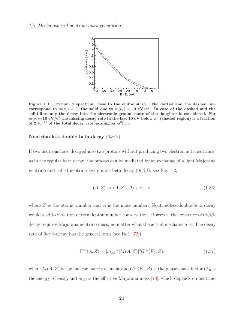
1.5 Mechanisms of neutrino mass generation
Figure 1.1. Tritium β spectrum close to the endpoint E0. The dotted and the dashed linecorrespond to m(νe) = 0, the solid one to m(νe) = 10 eV/c2. In case of the dashed and thesolid line only the decay into the electronic ground state of the daughter is considered. Form(νe)=10 eV/c2 the missing decay rate in the last 10 eV below E0 (shaded region) is a fractionof 2·10−10 of the total decay rate, scaling as m3(νe).
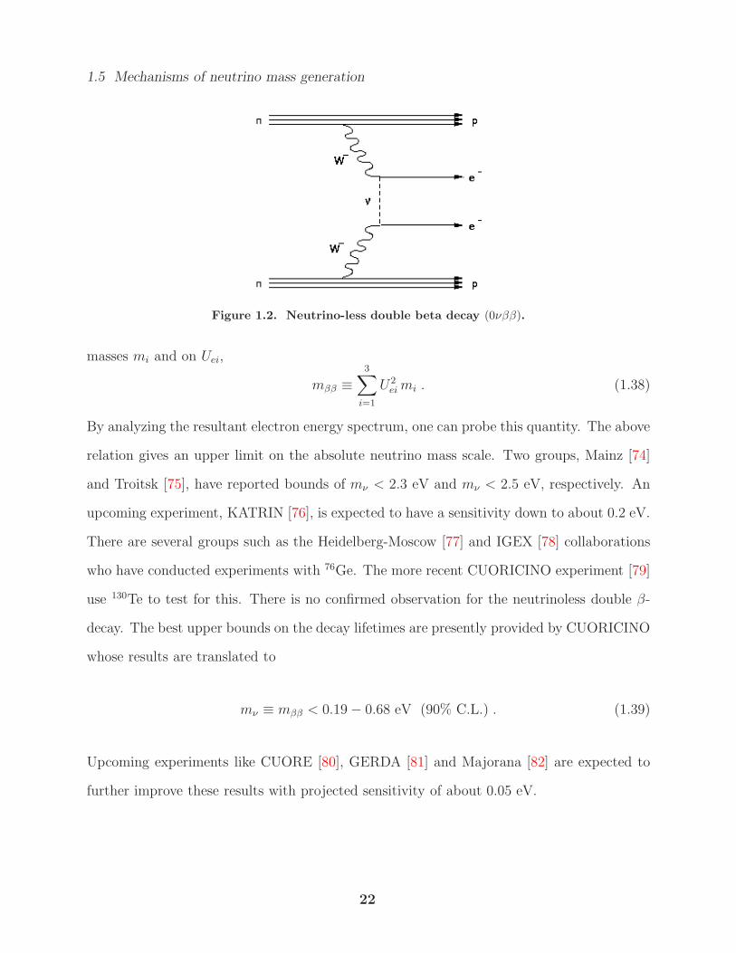
Neutrino-less double beta decay (0νββ)
If two neutrons have decayed into two protons without producing two electron anti-neutrinos,
as in the regular beta decay, the process can be mediated by an exchange of a light Majorana
neutrino and called neutrino-less double beta decay (0νββ), see Fig. 1.2,
(A,Z) → (A,Z + 2) + e + e, (1.36)
where Z is the atomic number and A is the mass number. Neutrinoless double-beta decay
would lead to violation of total lepton number conservation. However, the existence of 0νββ-
decay requires Majorana neutrino mass, no matter what the actual mechanism is. The decay
rate of 0νββ-decay has the general form (see Ref. [72])
Γ0ν(A,Z) = |mββ|2|M(A,Z)|2G0ν(E0, Z), (1.37)
whereM(A,Z) is the nuclear matrix element and G0ν(E0, Z) is the phase-space factor (E0 is
the energy release), and mββ is the effective Majorana mass [73], which depends on neutrino
21
1.5 Mechanisms of neutrino mass generation
Figure 1.2. Neutrino-less double beta decay (0νββ).
masses mi and on Uei,
mββ ≡3∑
i=1
U2eimi . (1.38)
By analyzing the resultant electron energy spectrum, one can probe this quantity. The above
relation gives an upper limit on the absolute neutrino mass scale. Two groups, Mainz [74]
and Troitsk [75], have reported bounds of mν < 2.3 eV and mν < 2.5 eV, respectively. An
upcoming experiment, KATRIN [76], is expected to have a sensitivity down to about 0.2 eV.
There are several groups such as the Heidelberg-Moscow [77] and IGEX [78] collaborations
who have conducted experiments with 76Ge. The more recent CUORICINO experiment [79]
use 130Te to test for this. There is no confirmed observation for the neutrinoless double β-
decay. The best upper bounds on the decay lifetimes are presently provided by CUORICINO
whose results are translated to
mν ≡ mββ < 0.19− 0.68 eV (90% C.L.) . (1.39)
Upcoming experiments like CUORE [80], GERDA [81] and Majorana [82] are expected to
further improve these results with projected sensitivity of about 0.05 eV.
22
1.5 Mechanisms of neutrino mass generation
Neutrino masses from cosmology
During the epoch of structure formation, free-streaming neutrinos with a large mass is as-
sumed to have significant effects on the growth of structure and, consequently, on the eventual
galaxy power spectrum. Thus, an accurate measurement of neutrinos could help put limits
on the scale of absolute neutrino mass given by the standard theory of structure forma-
tion. Studying the data from the Wilkinson Microwave Anisotropy Probe (WMAP) and the
Sloan Digital Sky Survey (SDSS) has found that the sum of neutrino masses, assuming three
species, is constrained by∑
i |mi| . 0.6 [83] and 1.6 eV [84], respectively, at a confidence
level of about 95%. Since the observed squared-mass splittings (∆m212,∆m
223) imply that
|mi−mj | ≪ O(0.1) eV for any i and j, taking∑
i |mi| . 0.6 gives an absolute upper bound
for each individual neutrino mass of about
|mi| . 0.2 eV (95% C.L.) for all i . (1.40)
This estimation agrees with the least upper bound imposed by the CUORICINO experiment,
which further confirms that the absolute neutrino mass scale must be in the sub-eV range.
1.5.2 See-saw mechanism
Neutrinos are extremely light and, hence, this might suggest a unique mass generation mecha-
nism to explain the smallness of mass in a natural way. The first reasonable attempt, see-saw
mechanism, was between late 1970’s and early 1980’s [85]. One of the simplest way to extend
the SM to accommodate neutrino masses is to introduce right-handed (RH) components νR
for neutrinos. The Dirac mass term for neutrinos is written as 12mDνLνR + h.c.. This is
not the only term allowed for neutrino masses. Since neutrinos are neutral particles, the
RH components are singlets under all the SM gauge symmetries. Thus, the Majorana mass
term 12MR(νR)cνR + h.c. is allowed, where the superscript c denotes charge conjugation, see
23
1.5 Mechanisms of neutrino mass generation
appendix A. The overall mass term for neutrinos can then be written in a matrix form as
Lmass = −1
2
(νL (νR)c
)
0 mD
mD MR
(νL)c
νR
+ h.c. (1.41)
Here, the above Lagrangian is assumed to be gauge invariant, thus, the upper left component
of the mass matrix is zero because it is not possible to add a Majorana mass term for left-
handed fields without breaking gauge invariance.
By assuming that the Majorana mass is much larger than the Dirac mass, i.e. MR ≫ mD,
diagonalizing the mass matrix yields the following two mass eigenvalues
mν∼= −mT
DM−1R mD, Mν
∼=MR. (1.42)
The first eigenvalue corresponds to a light neutrino mass while the second eigenvalue cor-
responds to the mass of a heavy Majorana neutrino. Roughly speaking, plugging a Dirac
mass at the electroweak scale, mD = 100 GeV, with a heavy neutrino mass close to the
unification scale, say MR = 1014 GeV, leads to a light neutrino mass of order mν = 0.1 eV.
This version of the see-saw mechanism with the additional RH neutrinos is referred to as
the type-I see-saw mechanism. The Lagrangian that describes this type can be written as
follows
Ltype-I = iνRiγµ∂µνRi − hαiℓLανRiΦ− 1
2MRi(νRi)cνRi + h.c. , (1.43)
where α = e, µ, τ , three new fields νRi, i = 1, 2, 3, a Majorana mass matrixMR and a Yukawa
coupling matrix h have been introduced. The effective interaction of the above Lagrangian
can schematically be described by the diagram in Fig. 1.3.
Instead of introducing right handed components to explain the neutrino masses, we could
24
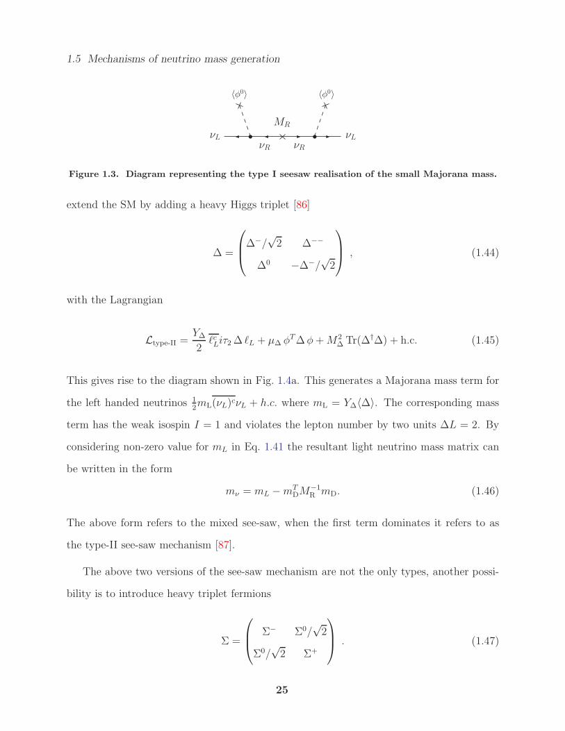
1.5 Mechanisms of neutrino mass generation
〈φ0〉〈φ0〉
νL νL
MR
νR νR
Figure 1.3. Diagram representing the type I seesaw realisation of the small Majorana mass.
extend the SM by adding a heavy Higgs triplet [86]
∆ =
∆−/
√2 ∆−−
∆0 −∆−/√2
, (1.44)
with the Lagrangian
Ltype-II =Y∆2ℓcLiτ2∆ ℓL + µ∆ φ
T∆φ+M2∆ Tr(∆†∆) + h.c. (1.45)
This gives rise to the diagram shown in Fig. 1.4a. This generates a Majorana mass term for
the left handed neutrinos 12mL(νL)cνL + h.c. where mL = Y∆〈∆〉. The corresponding mass
term has the weak isospin I = 1 and violates the lepton number by two units ∆L = 2. By
considering non-zero value for mL in Eq. 1.41 the resultant light neutrino mass matrix can
be written in the form
mν = mL −mTDM
−1R mD. (1.46)
The above form refers to the mixed see-saw, when the first term dominates it refers to as
the type-II see-saw mechanism [87].
The above two versions of the see-saw mechanism are not the only types, another possi-
bility is to introduce heavy triplet fermions
Σ =
Σ− Σ0/√2
Σ0/√2 Σ+
. (1.47)
25
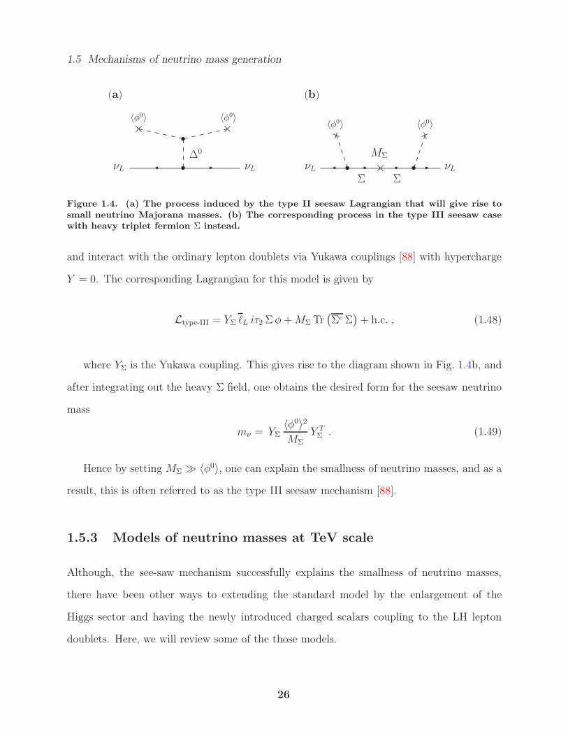
1.5 Mechanisms of neutrino mass generation
(a)
〈φ0〉〈φ0〉
νL νL
MΣ
Σ Σ
(b)
〈φ0〉〈φ0〉
νL νL
∆0
Figure 1.4. (a) The process induced by the type II seesaw Lagrangian that will give rise tosmall neutrino Majorana masses. (b) The corresponding process in the type III seesaw casewith heavy triplet fermion Σ instead.
and interact with the ordinary lepton doublets via Yukawa couplings [88] with hypercharge
Y = 0. The corresponding Lagrangian for this model is given by
Ltype-III = YΣ ℓL iτ2Σφ+MΣ Tr(Σc Σ
)+ h.c. , (1.48)
where YΣ is the Yukawa coupling. This gives rise to the diagram shown in Fig. 1.4b, and
after integrating out the heavy Σ field, one obtains the desired form for the seesaw neutrino
mass
mν = YΣ〈φ0〉2MΣ
Y TΣ . (1.49)
Hence by setting MΣ ≫ 〈φ0〉, one can explain the smallness of neutrino masses, and as a
result, this is often referred to as the type III seesaw mechanism [88].
1.5.3 Models of neutrino masses at TeV scale
Although, the see-saw mechanism successfully explains the smallness of neutrino masses,
there have been other ways to extending the standard model by the enlargement of the
Higgs sector and having the newly introduced charged scalars coupling to the LH lepton
doublets. Here, we will review some of the those models.
26
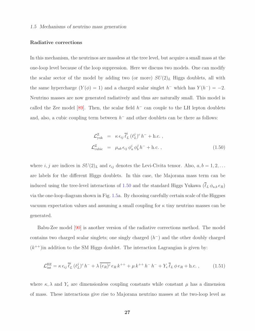
1.5 Mechanisms of neutrino mass generation
Radiative corrections
In this mechanism, the neutrinos are massless at the tree level, but acquire a small mass at the
one-loop level because of the loop suppression. Here we discuss two models. One can modify
the scalar sector of the model by adding two (or more) SU(2)L Higgs doublets, all with
the same hypercharge (Y (φ) = 1) and a charged scalar singlet h− which has Y (h−) = −2.
Neutrino masses are now generated radiatively and thus are naturally small. This model is
called the Zee model [89]. Then, the scalar field h− can couple to the LH lepton doublets
and, also, a cubic coupling term between h− and other doublets can be there as follows:
LZyuk = κ ǫij ℓ
i
L (ℓjL)
c h− + h.c. ,
LZcubic = µab ǫij φ
ia φ
jb h
− + h.c. , (1.50)
where i, j are indices in SU(2)L and ǫij denotes the Levi-Civita tensor. Also, a, b = 1, 2, . . .
are labels for the different Higgs doublets. In this case, the Majorana mass term can be
induced using the tree-level interactions of 1.50 and the standard Higgs Yukawa (ℓL φa,b eR)
via the one-loop diagram shown in Fig. 1.5a. By choosing carefully certain scale of the Higgses
vacuum expectation values and assuming a small coupling for κ tiny neutrino masses can be
generated.
Babu-Zee model [90] is another version of the radiative corrections method. The model
contains two charged scalar singlets; one singly charged (h−) and the other doubly charged
(k++)in addition to the SM Higgs doublet. The interaction Lagrangian is given by:
LBZint = κ ǫij ℓ
i
L (ℓjL)
c h− + λ (eR)c eR k++ + µ k++ h− h− + Ye ℓL φ eR + h.c. , (1.51)
where κ, λ and Ye are dimensionless coupling constants while constant µ has a dimension
of mass. These interactions give rise to Majorana neutrino masses at the two-loop level as
27
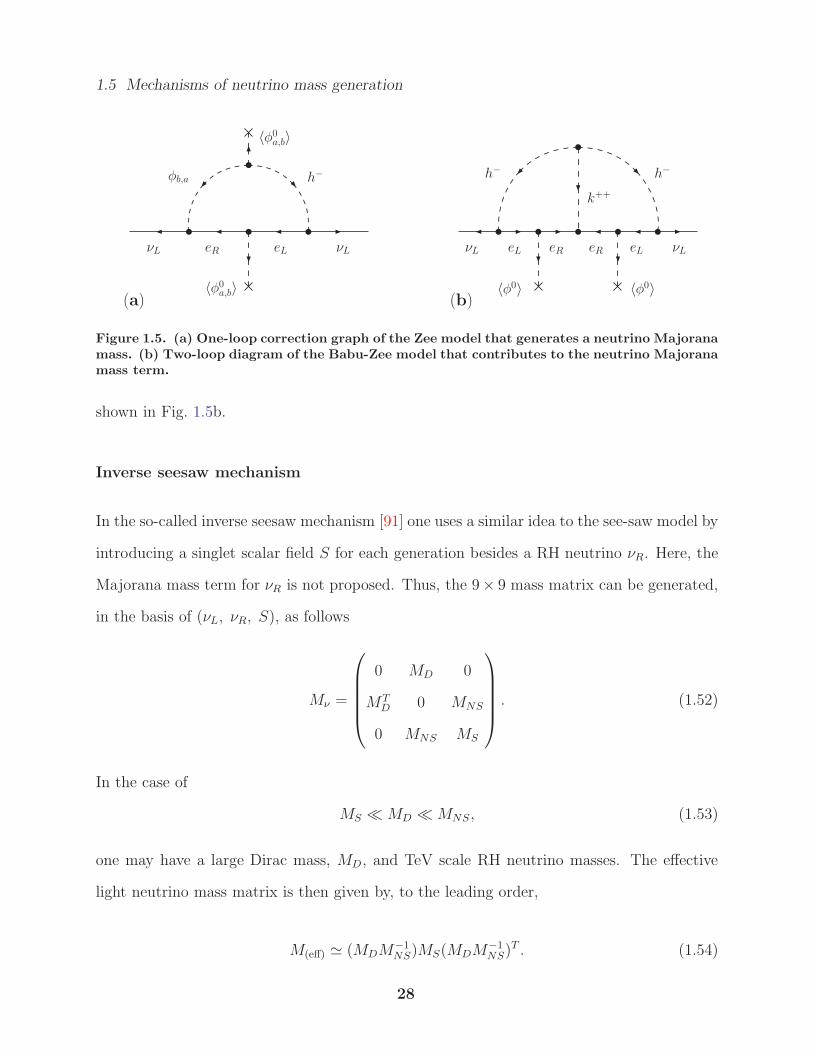
1.5 Mechanisms of neutrino mass generation
(a) (b)〈φ0
a,b〉
φb,a h−
eR eL νLνL νL νLeL eLeR eR
〈φ0〉 〈φ0〉
h− h−
k++
〈φ0a,b〉
Figure 1.5. (a) One-loop correction graph of the Zee model that generates a neutrino Majoranamass. (b) Two-loop diagram of the Babu-Zee model that contributes to the neutrino Majoranamass term.
shown in Fig. 1.5b.
Inverse seesaw mechanism
In the so-called inverse seesaw mechanism [91] one uses a similar idea to the see-saw model by
introducing a singlet scalar field S for each generation besides a RH neutrino νR. Here, the
Majorana mass term for νR is not proposed. Thus, the 9× 9 mass matrix can be generated,
in the basis of (νL, νR, S), as follows
Mν =
0 MD 0
MTD 0 MNS
0 MNS MS
. (1.52)
In the case of
MS ≪ MD ≪MNS, (1.53)
one may have a large Dirac mass, MD, and TeV scale RH neutrino masses. The effective
light neutrino mass matrix is then given by, to the leading order,
M(eff) ≃ (MDM−1NS)MS(MDM
−1NS)
T . (1.54)
28
1.6 Neutrino symmetries of nature
Thus, the smallness of the neutrino masses is due to the smallness of the lepton number
violation coupling, MS, which is lower than the EW scale. Viable effective neutrino masses
can be obtained with MNS ∼ O(1 TeV), MD ∼ O(100 GeV), and MS ∼ O(0.1 keV).
Higher dimensional operator approach
In the seesaw mechanism, the neutrino masses are generated by dimension-5 effective oper-
ators,
HHLL
∆. (1.55)
It is supposed that Majorana neutrino masses are generated at the cutoff scale of the new
physics which is commonly defined at the GUT scale in order to sufficiently suppress the
effective light neutrino masses. In the presence of some new symmetry, neutrino masses are
generated only at high mass dimensionalities while operators with lower mass dimensional-
ities are forbidden [92]. In this case, the operators generically have the suppression factor
in terms of some power p of the ratio of VEV of the scalar field, φ, that breaks the new
symmetry to the cutoff scale of the symmetry scale,(
〈φ〉∆
)p
. If the dimensionality is high
enough, the cutoff scale of the new physics can be on the order of a TeV.
1.6 Neutrino symmetries of nature
Symmetry is the main ingredient in particle physics to understand several phenomena.
Abelian as well as non-Abelian discrete symmetries are used in model building in order
to control allowed couplings and to study the flavor physics beyond the standard model.
The quark and lepton masses and mixing angles have been studied in the framework of
the flavor symmetries which are presented to control the Yukawa couplings. The study of
neutrino masses and mixing [93] has stimulated interests in flavor symmetries. Non-Abelian
discrete symmetries are studied as a tool for model building to derive experimental values
29
1.6 Neutrino symmetries of nature
of quark/lepton masses and mixing angles.
1.6.1 2-3 and Zn
The 2-3, or µ− τ , is a symmetry in which the matrix elements of the neutrino mass matrix
Mν is invariant under the interchange of the flavor basis vectors |e〉 ↔ |e〉 and |µ〉 ↔ −|τ〉.
The minus sign in this transformation is introduced to conventionally generate only positive
mixing angles. With this symmetry,
Meµν = −Meτ
ν ,
Mµµν = Mττ
ν ,
Mµτν = Mτµ
ν . (1.56)
Thus, we may parametrize Mν by four parameters as in
Mν =
a b −b
b f e
−b e f
. (1.57)
The two conditions in 1.56 implies s13 = 0 and s23 = 1/√2, and the unitary matrix that
diagonalize the mass matrix is equal to
U =
c12 s12 0
− 1√2s12
1√2c12
1√2
1√2s12 − 1√
2c12
1√2
=
1 0 0
0 1√2
1√2
0 − 1√2
1√2
·
c12 s12 0
−s12 c12 0
0 0 1
. (1.58)
The neutrino mass-squared difference values (∆m12)2 ≪ (∆m23)
2 demonstrate thatm1 ≈
m2 then it is much more natural to have a 1-2 symmetry [94] rather than a 2-3 symmetry.
30
1.6 Neutrino symmetries of nature
For this reason, the 2-3 symmetry in 1.56 might seem to be totally unnatural. Nevertheless,
it turns out that the 2-3 symmetry on Mν given by 1.56 places no restriction whatsoever on
the neutrino masses mi, so this 2-3 symmetry on Mν is not contradictory to a 1-2 symmetry
on the mass spectrum. Moreover, the 2-3 symmetry gives rise naturally to the right mixing
of neutrinos.
The suggested structure of the neutrino mass matrix in the 2-3 symmetric limit leads to
an additional symmetry of the mass matrix such as the Abelian discrete cyclic group Zn. The
Zn group is defined as the group of n elements A1, A2, . . . , An such that for each element
in the group Ani = I where I is the identity matrix. The Zn group can be represented as
discrete rotations, whose generator corresponds to 2π/n rotation. For example, the group
Z2 consists of two elements e, a where a2 = e. The transformation of the element a under
the Z2 group could be even or odd i.e. a → ±a. The Z4 group consists of four elements
e, a, b, c where a4 = b4 = c4 = e. The transformation of the Z4 symmetry in the standard
basis is given as x→ ±y or x→ ±iy for x, y = a, b, c.
1.6.2 A4
The A4 group is the symmetry of a tetrahedron as shown in Figure 1.6 and it is the smallest
non-Abelian group. All of the 12 elements of the A4 are denoted as
They are classified by the conjugacy classes as
C1 : a1, h = 1,
C3 : a2, a3, a4, h = 2,
C4 : b1, b2, b3, b4, h = 3,
C4′ : c1, c2, c3, c4, h = 3,
where we denote the orders of each element in the conjugacy class by h, where ah = e.
31
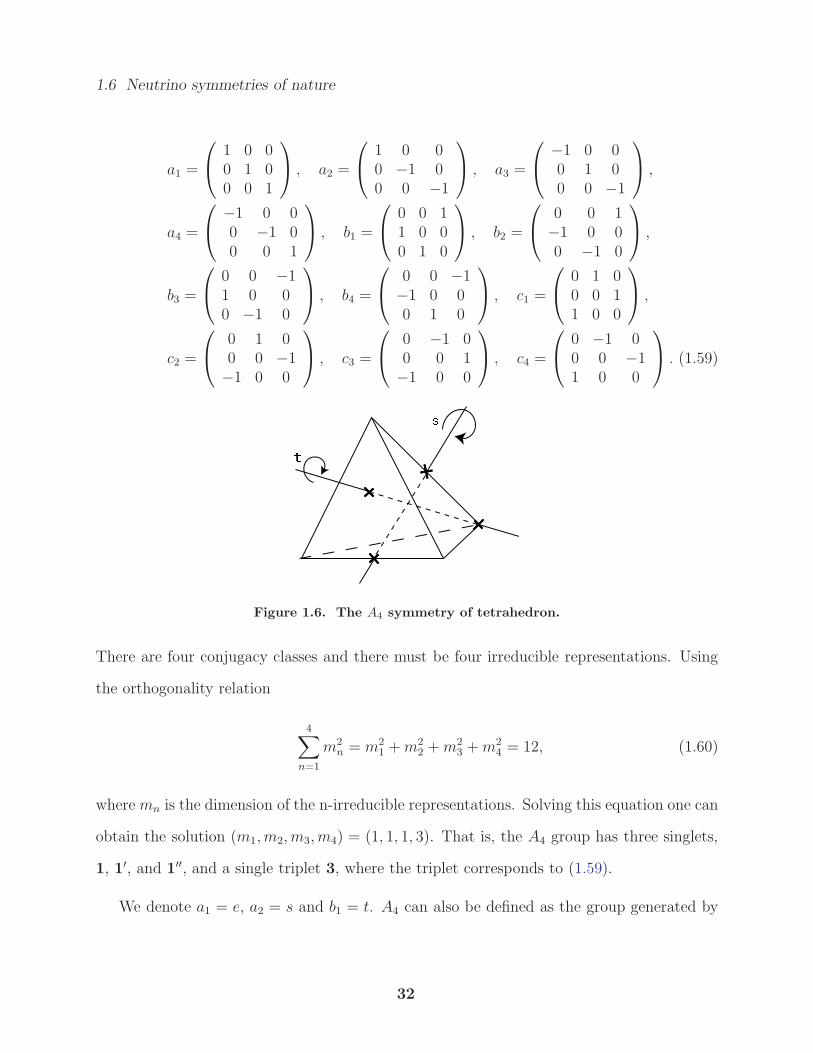
1.6 Neutrino symmetries of nature
a1 =
1 0 00 1 00 0 1
, a2 =
1 0 00 −1 00 0 −1
, a3 =
−1 0 00 1 00 0 −1
,
a4 =
−1 0 00 −1 00 0 1
, b1 =
0 0 11 0 00 1 0
, b2 =
0 0 1−1 0 00 −1 0
,
b3 =
0 0 −11 0 00 −1 0
, b4 =
0 0 −1−1 0 00 1 0
, c1 =
0 1 00 0 11 0 0
,
c2 =
0 1 00 0 −1−1 0 0
, c3 =
0 −1 00 0 1−1 0 0
, c4 =
0 −1 00 0 −11 0 0
. (1.59)
Figure 1.6. The A4 symmetry of tetrahedron.
There are four conjugacy classes and there must be four irreducible representations. Using
the orthogonality relation
4∑
n=1
m2n = m2
1 +m22 +m2
3 +m24 = 12, (1.60)
where mn is the dimension of the n-irreducible representations. Solving this equation one can
obtain the solution (m1, m2, m3, m4) = (1, 1, 1, 3). That is, the A4 group has three singlets,
1, 1′, and 1′′, and a single triplet 3, where the triplet corresponds to (1.59).
We denote a1 = e, a2 = s and b1 = t. A4 can also be defined as the group generated by
32
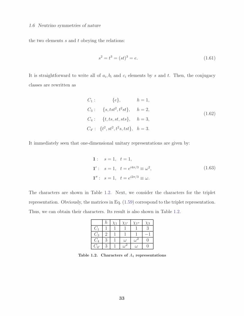
1.6 Neutrino symmetries of nature
the two elements s and t obeying the relations:
s2 = t3 = (st)3 = e. (1.61)
It is straightforward to write all of ai, bi and ci elements by s and t. Then, the conjugacy
classes are rewritten as
C1 : e, h = 1,
C3 : s, tst2, t2st, h = 2,
C4 : t, ts, st, sts, h = 3,
C4′ : t2, st2, t2s, tst, h = 3.
(1.62)
It immediately seen that one-dimensional unitary representations are given by:
1 : s = 1, t = 1,
1′ : s = 1, t = ei4π/3 ≡ ω2,
1′′ : s = 1, t = ei2π/3 ≡ ω.
(1.63)
The characters are shown in Table 1.2. Next, we consider the characters for the triplet
representation. Obviously, the matrices in Eq. (1.59) correspond to the triplet representation.
Thus, we can obtain their characters. Its result is also shown in Table 1.2.
h χ1 χ1′ χ1′′ χ3
C1 1 1 1 1 3C3 2 1 1 1 −1C4 3 1 ω ω2 0C4′ 3 1 ω2 ω 0
Table 1.2. Characters of A4 representations
33
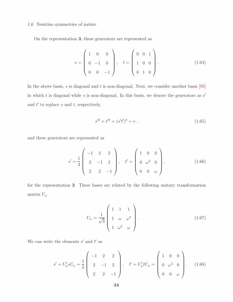
1.6 Neutrino symmetries of nature
On the representation 3, these generators are represented as
s =
1 0 0
0 −1 0
0 0 −1
, t =
0 0 1
1 0 0
0 1 0
. (1.64)
In the above basis, s is diagonal and t is non-diagonal. Next, we consider another basis [95]
in which t is diagonal while s is non-diagonal. In this basis, we denote the generators as s′
and t′ to replace s and t, respectively,
s′2 = t′3 = (s′t′)3 = e . (1.65)
and these generators are represented as
s′ =1
3
−1 2 2
2 −1 2
2 2 −1
, t′ =
1 0 0
0 ω2 0
0 0 ω
, (1.66)
for the representation 3. These bases are related by the following unitary transformation
matrix Uω
Uω =1√3
1 1 1
1 ω ω2
1 ω2 ω
. (1.67)
We can write the elements s′ and t′ as
s′ = U †ωsUω =
1
3
−1 2 2
2 −1 2
2 2 −1
, t′ = U †
ωtUω =
1 0 0
0 ω2 0
0 0 ω
. (1.68)
34
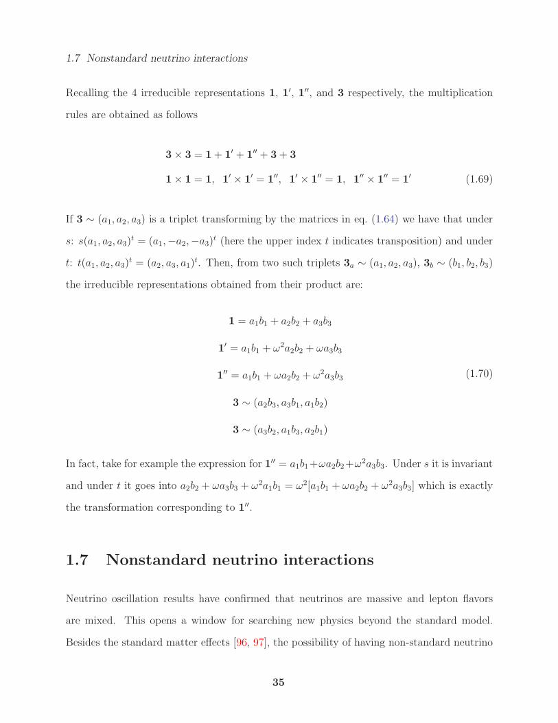
1.7 Nonstandard neutrino interactions
Recalling the 4 irreducible representations 1, 1′, 1′′, and 3 respectively, the multiplication
rules are obtained as follows
3× 3 = 1+ 1′ + 1′′ + 3+ 3
1× 1 = 1, 1′ × 1′ = 1′′, 1′ × 1′′ = 1, 1′′ × 1′′ = 1′ (1.69)
If 3 ∼ (a1, a2, a3) is a triplet transforming by the matrices in eq. (1.64) we have that under
s: s(a1, a2, a3)t = (a1,−a2,−a3)t (here the upper index t indicates transposition) and under
t: t(a1, a2, a3)t = (a2, a3, a1)
t. Then, from two such triplets 3a ∼ (a1, a2, a3), 3b ∼ (b1, b2, b3)
the irreducible representations obtained from their product are:
1 = a1b1 + a2b2 + a3b3
1′ = a1b1 + ω2a2b2 + ωa3b3
1′′ = a1b1 + ωa2b2 + ω2a3b3
3 ∼ (a2b3, a3b1, a1b2)
3 ∼ (a3b2, a1b3, a2b1)
(1.70)
In fact, take for example the expression for 1′′ = a1b1+ωa2b2+ω2a3b3. Under s it is invariant
and under t it goes into a2b2 + ωa3b3 + ω2a1b1 = ω2[a1b1 + ωa2b2 + ω2a3b3] which is exactly
the transformation corresponding to 1′′.
1.7 Nonstandard neutrino interactions
Neutrino oscillation results have confirmed that neutrinos are massive and lepton flavors
are mixed. This opens a window for searching new physics beyond the standard model.
Besides the standard matter effects [96, 97], the possibility of having non-standard neutrino
35
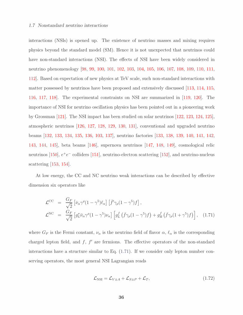
1.7 Nonstandard neutrino interactions
interactions (NSIs) is opened up. The existence of neutrino masses and mixing requires
physics beyond the standard model (SM). Hence it is not unexpected that neutrinos could
have non-standard interactions (NSI). The effects of NSI have been widely considered in
neutrino phenomenology [98, 99, 100, 101, 102, 103, 104, 105, 106, 107, 108, 109, 110, 111,
112]. Based on expectation of new physics at TeV scale, such non-standard interactions with
matter possessed by neutrinos have been proposed and extensively discussed [113, 114, 115,
116, 117, 118]. The experimental constraints on NSI are summarized in [119, 120]. The
importance of NSI for neutrino oscillation physics has been pointed out in a pioneering work
by Grossman [121]. The NSI impact has been studied on solar neutrinos [122, 123, 124, 125],
atmospheric neutrinos [126, 127, 128, 129, 130, 131], conventional and upgraded neutrino
beams [132, 133, 134, 135, 136, 103, 137], neutrino factories [133, 138, 139, 140, 141, 142,
143, 144, 145], beta beams [146], supernova neutrinos [147, 148, 149], cosmological relic
neutrinos [150], e+e− colliders [151], neutrino-electron scattering [152], and neutrino-nucleus
scattering [153, 154].
At low energy, the CC and NC neutrino weak interactions can be described by effective
dimension six operators like
LCC =GF√2
[ναγ
ρ(1− γ5)ℓα] [f ′γρ(1− γ5)f
],
LNC =GF√2
[gνLναγ
ρ(1− γ5)να] [gfL
(fγρ(1− γ5)f
)+ gfR
(fγρ(1 + γ5)f
)], (1.71)
where GF is the Fermi constant, να is the neutrino field of flavor α, ℓα is the corresponding
charged lepton field, and f , f ′ are fermions. The effective operators of the non-standard
interactions have a structure similar to Eq. (1.71). If we consider only lepton number con-
serving operators, the most general NSI Lagrangian reads
LNSI = LV±A + LS±P + LT , (1.72)
36
1.7 Nonstandard neutrino interactions
where the different terms are classified according to their Lorentz structure in the following
way:
LV±A =GF√2
∑
f,f ′
εf,f′,V±A
αβ
[νβγ
ρ(1− γ5)ℓα] [f ′γρ(1± γ5)f
]
+GF√2
∑
f
εf,V±Aαβ
[ναγ
ρ(1− γ5)νβ][fγρ(1± γ5)f
]+ h.c.,
LS±P =GF√2
∑
f,f ′
εf,f′,S±P
αβ
[νβ(1 + γ5)ℓα
][f ′(1± γ5)f
],
LT =GF√2
∑
f,f ′
εf,f′,T
αβ [νβσρτ ℓα]
[f ′σρτf
]. (1.73)
The dimensionless NSI parameters ε’s represent the strength of the nonstandard interactions
relative to GF . Note that we deal with the SM neutrinos which are purely left-handed
particles. This constraint on the neutrino chirality forbids ννff terms in LS±P and LT . If
the nonstandard interactions are supposed to be mediated by new state with a mass of order
MNSI, the effective vertices in Eq. (1.73) will be suppressed by 1/M2NSI in the same way as
the standard weak interactions are suppressed by 1/M2W. Therefore we expect that
|ε| ∼ M2W
M2NSI
. (1.74)
NSI effects enter the neutrino oscillation at production, propagation, and detection pro-
cesses. For simplicity, we are going to discuss the NSI effect by considering the following
effective weak interaction
LNSI =GF√2
∑
f,P
εfPαβ (ναγµLνβ)
(fγµPf
), (1.75)
where P = L,R is a projection operator. In order to introduce the effective mixing pa-
rameters in the presence of the non-standard interactions, we start from neutrino oscillations
37
1.7 Nonstandard neutrino interactions
in vacuum. The evolution in time of a neutrino mass eigenstate |ν(t)〉 can be described by
id
dt|ν(t)〉 = H|ν(t)〉 , (1.76)
where H is the Hamiltonian of the system. For neutrinos traveling in vacuum, the Hamilto-
nian in the ultra-relativistic limit E ≫ mi is
H =1
2EUdiag
(0,∆m2
21,∆m231
)U † , (1.77)
Thus, the neutrino oscillation probability from a neutrino flavor α to a neutrino flavor β is
given by
Pαβ ≡ |Sαβ(t, t0)|2 =∣∣∣∣∣∑
i
UβiU∗αie
−im2
i L
2E
∣∣∣∣∣
2
. (1.78)
The effective Hamiltonian responsible for neutrino propagation in matter, disregarding the
neutral current contributions, is given by
Hαβ = Hαβ + a (δαeδβe + εαβ) , (1.79)
where a =√2GFNe is the matter parameter arises from coherent forward scattering, Ne
denotes the electron number density along the neutrino trajectory in matter, and the NSI
parameters εαβ are defined as
εαβ =∑
f,P
εfPαβNf
Ne
, (1.80)
with Nf being the number density of a fermion of type f . The effective Hamiltonian in
38
1.7 Nonstandard neutrino interactions
matter can be written similar to the vacuum Hamiltonian in Eq. (1.77) as
H =1
2EUdiag
(m2
1, m22, m
23
)U † , (1.81)
where m2i denote the effective mass-squared eigenvalues of neutrinos and U is the unitary
mixing matrix in matter. Assuming a constant matter density profile, which is close to reality,
one can obtain the transition probability with matter effects including the NSI contribution
Pαβ ≡ |Sβα(t, t0)|2 =∣∣∣∣∣∑
i
U∗βiUαie
−im2
i L
2E
∣∣∣∣∣
2
. (1.82)
From Eqs. (1.78, 1.82), the neutrino oscillation probability in vacuum and in matter have the
same form with replacing the vacuum parameters U and m2i by the effective parameters U
and m2i . Thus, the key point turns out to be the diagonalization of the effective Hamiltonian
H and figuring out the explicit relations of the effective parameters.
After discussing the NSI effects in the propagation process of neutrinos, now in order to
complete the picture we need to introduce the contributions of the NSIs at the production
and detection processes. In most of the viable models for NSIs, the source and detector
effects are simultaneously taken into account. Now, the NSI parameters at sources and
detectors can be defined as [155, 138, 156]
|νsα〉 = |να〉+∑
β=e,µ,τ
εsαβ|νβ〉 = (1 + εs)U |νi〉 , (1.83)
〈νdβ| = 〈νβ|+∑
α=e,µ,τ
εdαβ〈να| = 〈νi|U †[1 + (εd)†] , (1.84)
where the superscripts ‘s’ and ‘d’ denote source and detector, respectively, and |νi〉 is a
neutrino mass eigenstate. Note that the states |νsα〉 and 〈νdβ| are not orthonormal states due
to the NSIs. The matrices εs and εd are arbitrary and non-unitary in general. They are not
necessarily the same matrix since different physical processes take place at the source and
39
1.7 Nonstandard neutrino interactions
the detector. If the production and detection processes are exactly the same process with
the same participating fermions (e.g. β-decay and inverse β-decay), then the same matrix
enters as εs =(εd)†, or on the form of matrix elements, εsαβ = εdαβ = (εsβα)
∗ = (εdβα)∗ [156].
For example, in the case of non-unitarity effects (which can be considered as a type of NSIs,
see e.g. Ref. [157]) in the minimal unitarity violation model [158, 159, 160, 161, 162, 163]
εs =(εd)†. Thus, it is important to keep in mind that these matrices are model-dependent
parameters.
The transition probabilities are then modified in general as2
Pαβ =
∣∣∣∣[(1 + εd
)T · S(t, t0) · (1 + εs)T]βα
∣∣∣∣2
,
=
∣∣∣∣∣∑
γ,δ,i
(1 + εd
)γβ
(1 + εs)αδ UδiU∗γie
−im2
i L
2E
∣∣∣∣∣
2
,
=∑
i,j
J iαβJ j∗
αβ − 4∑
i>j
Re(J iαβJ j∗
αβ) sin2
(∆m2
ijL
4E
)
+ 2∑
i>j
Im(J iαβJ j∗
αβ) sin
(∆m2
ijL
2E
), (1.85)
where
J iαβ = U∗
αiUβi +∑
γ
εsαγU∗γiUβi +
∑
γ
εdγβU∗αiUγi +
∑
γ,δ
εsαγεdδβU
∗γiUδi . (1.86)
In fact, an important feature of Eq. (1.85) is that when α 6= β, the first term is generally
non-vanishing, which means that a neutrino flavor transition would already happen at the
source before the oscillation process has taken place. This is known as the zero-distance effect
[164]. It could be measured with a near detector close to the source. Note that Eq. (1.85)
is also usable to describe neutrino oscillations with a non-unitary mixing matrix, e.g. in the
minimal unitarity violation model [158].
2Here we have neglected the normalization factors, which are needed in order to normalize the quantumstates.
40
Chapter 2
Probing Light Pseudoscalar, Axial Vector
States Through ηb → τ+τ−
2.1 Introduction
In this work we will be interested in probing light scalar and spin 1 states via ηb decays. As
the ηb is a pseudoscalar, a light pseudoscalar and a spin 1 state with axial vector coupling can
directly couple to ηb. We will assume the pseudoscalar to couple to the mass of the fermion
as is usually the case for Higgs coupling to fermions. Hence, the ηb which is a bb bound state
has advantages over the ηc and η/η′ mesons which are cc and qq(q = u, d, s) bound states,
respectively. The ηb is expected to be a sensitive probe of a light axial vector state. This
follows from the fact that the longitudinal polarization of the axial vector, ǫµL ∼ kµ, when kµ
the momentum of the vector boson is much larger than its mass. Consequently, the effective
axial vector-fermion pair coupling is proportional to the fermion mass for the longitudinal
polarization.
In this work we will study the process ηb → τ+τ− mediated by a pseudoscalar (A0)
or an axial vector (U). In the SM this process can only go through a Z exchange at tree
level and is highly suppressed with a branching ratio ∼ 4 × 10⁻⁹. There is also a higher
order contribution to ηb → τ+τ− in the SM, via two intermediate photons. The branching
ratio for this process is also tiny ∼ 10−10. Hence, a measurement of BR[ηb → τ+τ−] larger
than the SM rate will be a signal of new states. One can also probe the states A0(U) in Υ
decays. To search for light A0(U) states in Υ decays one generally considers the decay chains,
Υ → A0(U)γ (A0(U) → τ+τ−) [21]. In other words, the A0(U) is assumed to be produced
41
2.1 Introduction
on-shell. One then looks for a peak in the invariant mass of the τ pairs. The experimental
measurement/constraint of BR[Υ → A0(U)γ]×BR[A0(U) → τ+τ−] can be converted into a
measurement/constraint on the coupling of the A0(U) to bb, and hence on model parameters,
if the BR[A0(U) → τ+τ−] is used as an input [165]. Clearly as mA0(U) > mΥ, the A0(U) can
no longer be produced on-shell and the rate for Υ → τ+τ−γ will fall and consequently the
constraints on the model parameters will be weaker. Note that the constraint mA0 < 2mB
needs to be assumed in the very particular case where the CP -even Higgs mass mh < 114
GeV and h → 2A0 dominates over h → 2mb [11]. In general mA0 > 2mB is also possible.
We will just assume the existence of light pseudoscalar and axial vector states close to the
ηb mass but they can have masses that are greater than or less than 2mb.
The ηb has only been seen in the radiative decays Υ → γηb. Hence, the decay ηb → τ+τ−
has only been studied via the decay Υ → τ+τ−γ. However, the decay ηb → τ+τ− can be
studied independently from the process Υ → τ+τ−γ as the ηb can be produced from various
other processes such as two-photon collisions, γγ → ηb [16], and in two parton collisions
[17, 166], in hadron colliders like the Tevatron and the LHC. The process ηb → τ+τ− has
several advantages over Υ decays in probing A0(U) states specially when A0(U) is off-shell
which is always the case when mA0(U) > mΥ. First, unlike the ηb which can couple directly to
A0(U), the Υ can only couple to A0(U) in conjunction with another state- usually a photon.
Hence, the Υ couplings are second order and therefore it can decay only to the τ+τ−γ
state with a rate much smaller than the rate for ηb → τ+τ−. However, the Υ states are
narrower than the ηb, which may compensate partially the larger rate for ηb → τ+τ− relative
to Υ → τ+τ−γ in the branching ratio measurements. Secondly, an important distinction
between Υ → τ+τ−γ and ηb → τ+τ− is that the former decay can also proceed as a radiative
decay in the SM while the latter decay is highly suppressed in the SM as indicated above.
Adapting the expression used to estimate the SM branching ratio for J/ψ → e+e−γ [167],
with the γ emitted from the final state electrons, to the decay Υ → τ+τ−γ, the rate for this
42
2.1 Introduction
decay in the SM is,
dΓΥ→τ+τ−γ = dΓΥ→τ+τ−β′32α
π
dE ′γ
E ′γ
s′
s
1− cos2θ′γτ(1− β ′2cos2θ′γτ )
2dΩ′
γ , (2.1)
with
dΓΥ→τ+τ− =3
3 + λ(1 + λ cos2 θ′τ )ΓΥ→τ+τ−
dΩ′τ
4π. (2.2)
Here E ′γ represents the γ energy, θ′γ and φ′
γ(Ω′γ) the γ angles, and θ′τ and φ′
τ (Ω′τ ) the τ angles,
all in the τ+τ− c.m. frame. β ′ is the τ velocity and θ′γτ is the angle between the τ and γ
directions, also in the τ+τ− c.m. frame while s′ is the τ+τ− invariant mass squared and s is
the Υ invariant mass squared. The parameter λ is determined from the experimental data
to be (0.88 ± 0.19) [167]. Using the branching ratio for Υ → τ+τ− = 2.6 × 10⁻² [168] we
estimate the branching ratio for Υ → τ+τ−γ = 4.4× 10⁻³ with Eγ > 100 MeV.
Naively, the rate for Υ → τ+τ−γ through an off-shell A0, from a 2HDM of type II,
relative to the SM rate for Υ → τ+τ−γ is ∼ g4 tan4 βm2bm
2τ
16e4M4W
. Therefore, for large tanβ ∼ 28
the SM and the NP rates may be comparable. However given the hadronic uncertainties
in estimating the SM and the NP rates for Υ → τ+τ−γ, it will be difficult to distinguish
between the NP and the SM contributions. Hence, searching for A0(U) with mA0(U) > mΥ
in Υ → τ+τ−γ will be very difficult because of the large SM background. Note that even in
e+e− machines like the B-factories where the ηb is produced through the decay Υ → γηb, the
product of branching ratios BR[Υ → γηb] × [ηb → τ+τ−] is tiny in the SM because of the
highly suppressed BR[ηb → τ+τ−] ∼ 4×10⁻⁹. Using the measured BR[Υ → γηb] ∼ 5×10⁻⁴
[12, 13] one obtains BR[Υ → γηb] × [ηb → τ+τ−] ∼ 2 × 10⁻¹² which is very difficult to
measure. In the presence of new physics this product of branching ratios is enhanced and
can reach <∼ 10−5. Hence the observation of Υ → γτ+τ−, with the τ pairs coming from
ηb, at branching ratios much larger than the SM expectations will be signal for new light
43
2.1 Introduction
states. In summary, the large SM background in Υ → τ+τ−γ and a tiny SM contribution
to ηb → τ+τ− makes the later decay potentially a better probe for A0(U) than the former if
the decays proceed through the off-shell exchange of A0(U).
There are good theoretical motivations for the existence of a light CP-odd A0 Higgs boson
or an axial vector boson U with masses, mA0 andmU respectively, in the GeV range or below.
There has been interest in the mA0 < 2mB region, for which a light Higgs, h, with SM-like
WW , ZZ and fermionic couplings can have mass mh ∼ 100 GeV while still being consistent
with LEP data by virtue of h→ A0A0. This scenario could even explain the 2.3 σ excess in
the e+e− → Z + 2b channel for M2b ∼ 100 GeV [169]. Such a light pseudoscalar Higgs can
naturally arise in extensions of MSSM with additional singlet scalars and fermions (gauge-
singlet supermultiplets) known as Next-to-Minimal Supersymmetric Model (NMSSM) [170].
Constraints on models with a light A0 state have been studied recently within a 2HDM
framework with certain assumptions about the coupling and in NMSSM [165, 171, 172].
Our goal will not be to work in a specific model but we will assume the couplings of the
A0 to the b quark and the τ lepton to be the same as in the 2HDM. We will assume this
2HDM is part of some extension of the SM. Hence, we will not strictly follow the bounds
and constraints obtained in some specific extension of the SM which includes the 2HDM,
but will choose values for the parameters in our calculation which are similar to constraints
on these parameters in specific NP models. The process ηb → τ+τ− will proceed through
an off-shell A0 and we will consider both mA0 < mηb and mA0 > mηb . In general, there will
be mixing between A0 and the ηb and as the pseudoscalar state gets close to the ηb mass
the mixing between the states will become important [173]. The calculation of this mixing
is model dependent and while there are estimates of this mixing in simple quark models
the mixing may be very different in other approaches to the bound state problem in QCD.
Hence, we will not take into account mixing in our analysis. Therefore, our results will be
reliable when the A0 mass is away from the ηb mass. We will further assume that the A0 is
44
2.2 ηb → τ+τ− in the SM and NP
narrow and neglect its width in our calculations. This approximation will be good as long as
mA0 is sufficiently away from the ηb mass. When A0 is produced on-shell both mixing and
width effects will become important and our results will not be reliable.
There are also models, for example within SUSY with extra gauged U(1), which have a
light axial vector state [174]. These light states can also mediate the process ηb → τ+τ−.
Constraints on these models have been studied [175, 176, 177, 178, 179]. We will consider
ηb → τ+τ− through the exchange of the axial vector U . To perform our calculations we
will choose the model discussed in [176, 179] and neglect the width of the U -boson. Fi-
nally, we note that there are recent dark matter models [180] that also contain light scalar
(pseudoscalar) and vector (axial vector) states which may be probed via ηb → τ+τ−. The
HyperCP collaboration has some events for the decay Σ+ → pµ+µ− which may be interpreted
as evidence for a light pseudoscalar state [181]. In this work we perform the calculations of
the decay ηb → τ+τ− in the SM and in models with a light pseudoscalar A0 and a light axial
vector U state. Next, we present our conclusion after the numerical results of the branching
ratios for ηb → τ+τ−.
2.2 ηb → τ+τ− in the SM and NP
In this section we will study ηb → τ+τ− in the SM and in models of NP. The ηb is a
pseudoscalar and cannot couple to γ directly. Hence, in the SM, ηb → τ+τ− can only
proceed through the exchange of a Z at tree level and we will calculate the branching ratio
for this process in the SM . This decay can also proceed at higher order in the SM through
intermediate two photon states.
In the presence of NP ηb → τ+τ− can proceed through the exchange of a light pseu-
doscalar or a light spin 1 boson with axial vector coupling. We will consider these two NP
scenarios in this section. The various tree level contribution to the ηb → τ+τ− in the SM
45
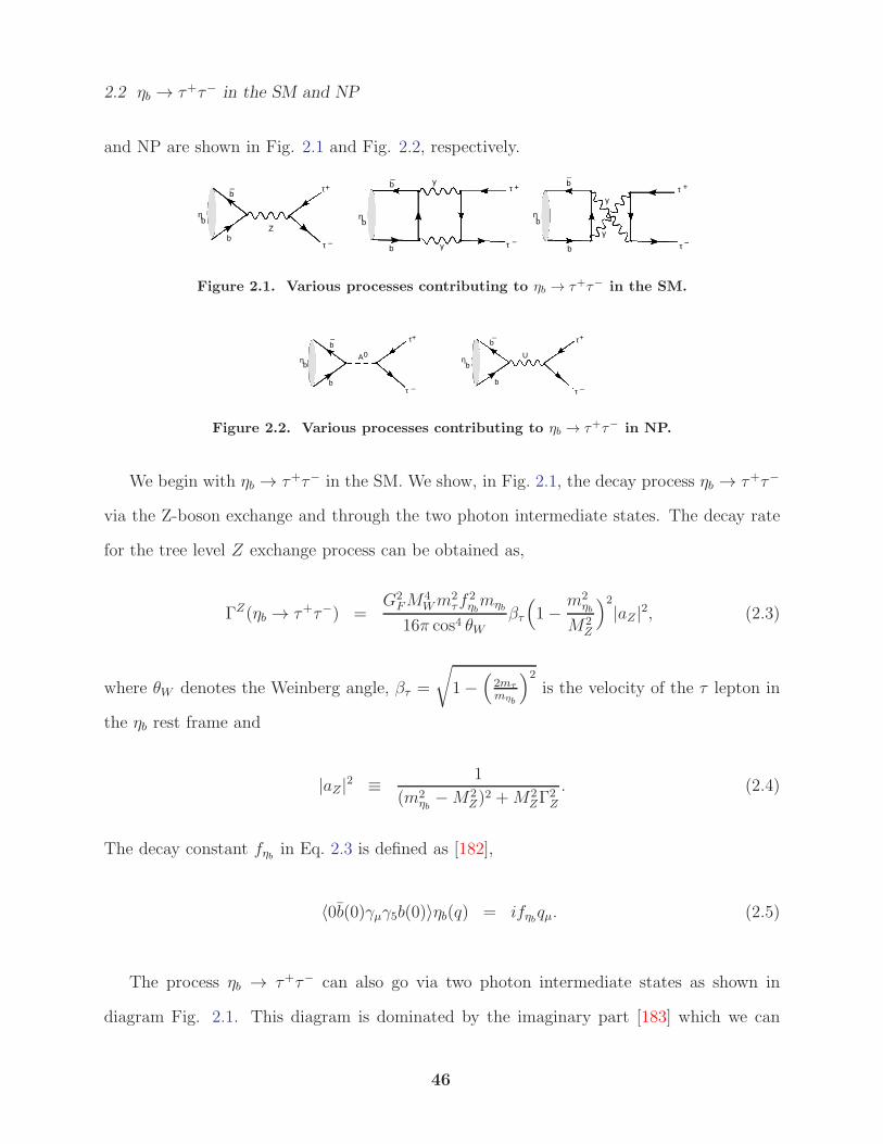
2.2 ηb → τ+τ− in the SM and NP
and NP are shown in Fig. 2.1 and Fig. 2.2, respectively.
Zb
b_ τ+
τ −
τ +
τ −b
b_
+τ
τ −
η η ηb b b
γ
γ
γ
γ
b
b_
Figure 2.1. Various processes contributing to ηb → τ+τ− in the SM.
A0ηb
τ+
τ_
b
b
_b_
b
bη
τ_
τ+
U
Figure 2.2. Various processes contributing to ηb → τ+τ− in NP.
We begin with ηb → τ+τ− in the SM. We show, in Fig. 2.1, the decay process ηb → τ+τ−
via the Z-boson exchange and through the two photon intermediate states. The decay rate
for the tree level Z exchange process can be obtained as,
ΓZ(ηb → τ+τ−) =G2
FM4Wm
2τf
2ηbmηb
16π cos4 θWβτ
(1−
m2ηb
M2Z
)2
|aZ|2, (2.3)
where θW denotes the Weinberg angle, βτ =
√1−
(2mτ
mηb
)2
is the velocity of the τ lepton in
the ηb rest frame and
|aZ|2 ≡ 1
(m2ηb−M2
Z)2 +M2
ZΓ2Z
. (2.4)
The decay constant fηb in Eq. 2.3 is defined as [182],
〈0b(0)γµγ5b(0)〉ηb(q) = ifηbqµ. (2.5)
The process ηb → τ+τ− can also go via two photon intermediate states as shown in
diagram Fig. 2.1. This diagram is dominated by the imaginary part [183] which we can
46
2.2 ηb → τ+τ− in the SM and NP
estimate using unitarity [184] to obtain,
Γ2γ [ηb → τ+τ−] ≥ α2
2βτ
[mτ
mηb
ln(1 + βτ )
(1− βτ )
]2Γ[ηb → γγ], (2.6)
where α is the electromagnetic fine structure constant. One can calculate Γ[ηb → γγ] as,
Γ[ηb → γγ] =πα2mηbf
2ηb
81m2b
, (2.7)
where we have used the heavy quark limit for the b quark. Since the 2γ exchange con-
tribution is mostly imaginary relative to the Z exchange contribution therefore to a good
approximation the total width Γt[ηb → τ+τ−] is ,
Γt[ηb → τ+τ−] ≈ ΓZ [ηb → τ+τ−] + Γ2γ [ηb → τ+τ−]. (2.8)
We now turn to NP models and begin with the 2HDM. The couplings of the down-type
quarks D and charged leptons ℓ with A0 in the generic 2HDM model are given by [185]
LD,ℓA0 =
igFA0
2MW(DMdiag
D γ5D + ℓMdiagl γ5ℓ)A
0, (2.9)
where FA0 is a model-dependent parameter, MdiagD = (md, mc, mb) andM
diagℓ = (me, mµ, mτ )
are the diagonal mass matrices of D and ℓ, respectively. We will consider FA0 > 1 in our
analysis. In the case of 2HDM type (II) FA0 ≡ tanβ while in 2HDM type (I) FA0 ≡ − cotβ.
In Fig. 2.2(a) we show the decay process ηb → τ+τ− via the exchange of the CP -odd
Higgs scalar A0. The decay rate for this process can be obtained as,
ΓA0
(ηb → τ+τ−) =G2
Fm2τf
2ηbm5
ηb
16πβτ |aA0|2, (2.10)
47
2.2 ηb → τ+τ− in the SM and NP
where the invariant coefficient aA0 depends on the mass mA0 as,
|aA0|2 ≡ F 4A0
(m2ηb−m2
A0)2. (2.11)
We have assumed that the decay width ΓA0 for the A0 is negligible. In Eq. 2.10, we have
used,
〈0b(0)γ5b(0)〉ηb(q) =ifηbm
2ηb
2mb, (2.12)
where fηb has been defined in Eq. 2.5.
Finally, we move to NP models that contain a light spin 1 boson with axial vector
couplings. In Fig. 2.2(b) we show the decay process ηb → τ+τ− via the exchange of the
light neutral gauge boson U . We write down a model independent Lagrangian for the U -
boson but we assume the structure of the Lagrangian to be similar to the one discussed in
Ref. [176, 177, 178]. We take the U couplings to the down-type quarks and charged leptons
to be given by
LD,ℓU = fD,ℓ
A (Dγµγ5D + ℓγµγ5ℓ)Uµ, (2.13)
with the axial coupling
fD,ℓA = 2−
34G
1
2
FmUFU , (2.14)
where mU denotes the mass of U -boson and FU denotes a model-dependent parameter. In
the specific model [176, 177, 178], FU ≡ cos ζ tan β.
Again, we will be interested in FU > 1. The decay rate for ηb → τ+τ− can be obtained
48
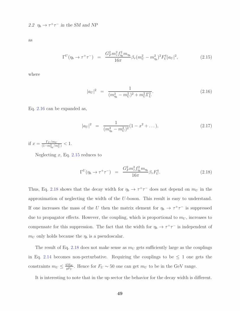
2.2 ηb → τ+τ− in the SM and NP
as
ΓU(ηb → τ+τ−) =G2
Fm2τf
2ηbmηb
16πβτ (m
2U −m2
ηb)2F 4
U |aU |2, (2.15)
where
|aU |2 =1
(m2ηb−m2
U)2 +m2
UΓ2U
. (2.16)
Eq. 2.16 can be expanded as,
|aU |2 =1
(m2ηb−m2
U)2(1− x2 + . . . ), (2.17)
if x = ΓU/mU
(1−m2ηb
/m2U )< 1.
Neglecting x, Eq. 2.15 reduces to
ΓU(ηb → τ+τ−) =G2
Fm2τf
2ηbmηb
16πβτF
4U . (2.18)
Thus, Eq. 2.18 shows that the decay width for ηb → τ+τ− does not depend on mU in the
approximation of neglecting the width of the U -boson. This result is easy to understand.
If one increases the mass of the U then the matrix element for ηb → τ+τ− is suppressed
due to propagator effects. However, the coupling, which is proportional to mU , increases to
compensate for this suppression. The fact that the width for ηb → τ+τ− is independent of
mU only holds because the ηb is a pseudoscalar.
The result of Eq. 2.18 does not make sense as mU gets sufficiently large as the couplings
in Eq. 2.14 becomes non-perturbative. Requiring the couplings to be ≤ 1 one gets the
constraints mU ≤ 4MW
gFU. Hence for FU ∼ 50 one can get mU to be in the GeV range.
It is interesting to note that in the up sector the behavior for the decay width is different.
49
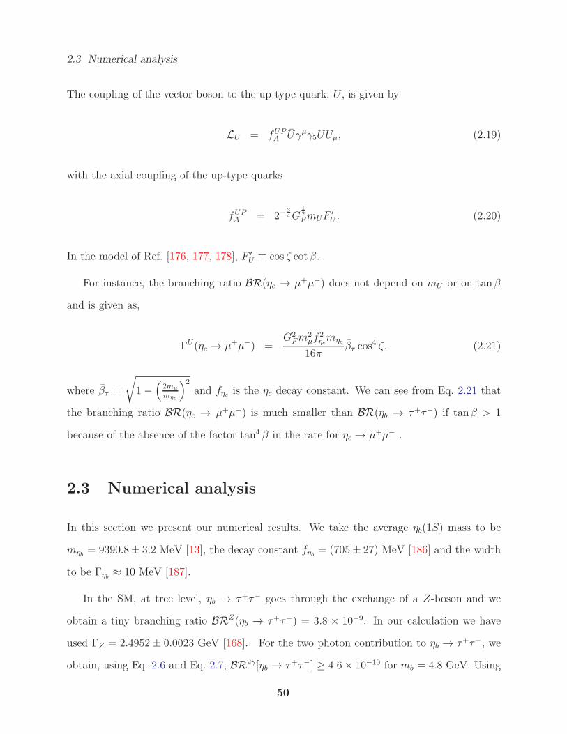
2.3 Numerical analysis
The coupling of the vector boson to the up type quark, U , is given by
LU = fUPA Uγµγ5UUµ, (2.19)
with the axial coupling of the up-type quarks
fUPA = 2−
34G
12
FmUF′U . (2.20)
In the model of Ref. [176, 177, 178], F ′U ≡ cos ζ cot β.
For instance, the branching ratio BR(ηc → µ+µ−) does not depend on mU or on tanβ
and is given as,
ΓU(ηc → µ+µ−) =G2
Fm2µf
2ηcmηc
16πβτ cos
4 ζ. (2.21)
where βτ =
√1−
(2mµ
mηc
)2
and fηc is the ηc decay constant. We can see from Eq. 2.21 that
the branching ratio BR(ηc → µ+µ−) is much smaller than BR(ηb → τ+τ−) if tanβ > 1
because of the absence of the factor tan4 β in the rate for ηc → µ+µ− .
2.3 Numerical analysis
In this section we present our numerical results. We take the average ηb(1S) mass to be
mηb = 9390.8± 3.2 MeV [13], the decay constant fηb = (705± 27) MeV [186] and the width
to be Γηb ≈ 10 MeV [187].
In the SM, at tree level, ηb → τ+τ− goes through the exchange of a Z-boson and we
obtain a tiny branching ratio BRZ(ηb → τ+τ−) = 3.8 × 10⁻⁹. In our calculation we have
used ΓZ = 2.4952± 0.0023 GeV [168]. For the two photon contribution to ηb → τ+τ−, we
obtain, using Eq. 2.6 and Eq. 2.7, BR2γ[ηb → τ+τ−] ≥ 4.6× 10⁻¹⁰ for mb = 4.8 GeV. Using
50
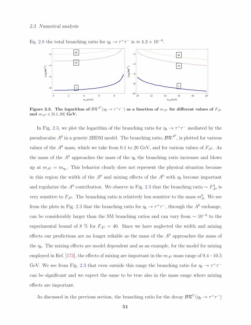
2.3 Numerical analysis
Eq. 2.8 the total branching ratio for ηb → τ+τ− is ≈ 4.3× 10⁻⁹.
1
20
40
0 2 4 6 8
-8
-6
-4
-2
mA0@GeVD
Log@B
RA
0D
1
20
40
10 12 14 16 18 20-10
-8
-6
-4
-2
mA0@GeVD
Log@B
RA
0D
Figure 2.3. The logarithm of BRA0
(ηb → τ+τ−) as a function of mA0 for different values of FA0
and mA0 ∈ [0.1, 20] GeV.
In Fig. 2.3, we plot the logarithm of the branching ratio for ηb → τ+τ− mediated by the
pseudoscalar A0 in a generic 2HDM model. The branching ratio, BRA0
, is plotted for various
values of the A0 mass, which we take from 0.1 to 20 GeV, and for various values of FA0 . As
the mass of the A0 approaches the mass of the ηb the branching ratio increases and blows
up at mA0 = mηb . This behavior clearly does not represent the physical situation because
in this region the width of the A0 and mixing effects of the A0 with ηb become important
and regularize the A0 contribution. We observe in Fig. 2.3 that the branching ratio ∼ F 4A0 is
very sensitive to FA0. The branching ratio is relatively less sensitive to the mass m0A. We see
from the plots in Fig. 2.3 that the branching ratio for ηb → τ+τ−, through the A0 exchange,
can be considerably larger than the SM branching ratios and can vary from ∼ 10−8 to the
experimental bound of 8 % for FA0 = 40. Since we have neglected the width and mixing
effects our predictions are no longer reliable as the mass of the A0 approaches the mass of
the ηb. The mixing effects are model dependent and as an example, for the model for mixing
employed in Ref. [173], the effects of mixing are important in themA0 mass range of 9.4−10.5
GeV. We see from Fig. 2.3 that even outside this range the branching ratio for ηb → τ+τ−
can be significant and we expect the same to be true also in the mass range where mixing
effects are important.
As discussed in the previous section, the branching ratio for the decay BRU(ηb → τ+τ−)
51
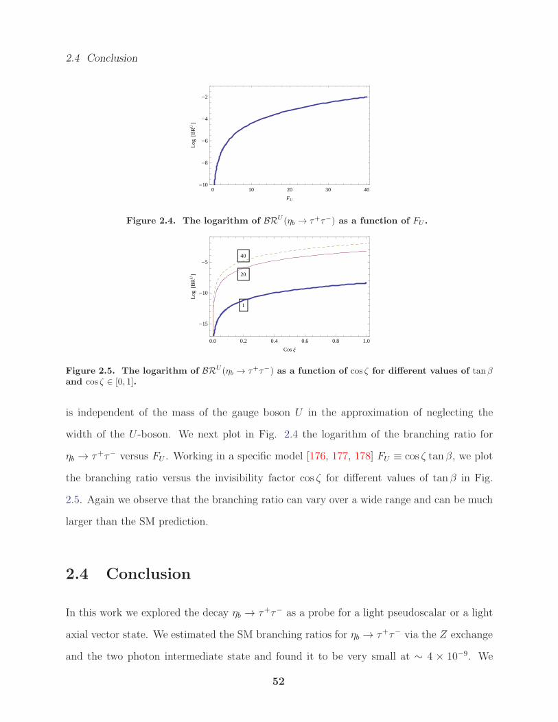
2.4 Conclusion
0 10 20 30 40-10
-8
-6
-4
-2
FU
Log@B
RUD
Figure 2.4. The logarithm of BRU (ηb → τ+τ−) as a function of FU .
1
20
40
0.0 0.2 0.4 0.6 0.8 1.0
-15
-10
-5
CosΞ
Log@B
RUD
Figure 2.5. The logarithm of BRU (ηb → τ+τ−) as a function of cos ζ for different values of tanβand cos ζ ∈ [0, 1].
is independent of the mass of the gauge boson U in the approximation of neglecting the
width of the U -boson. We next plot in Fig. 2.4 the logarithm of the branching ratio for
ηb → τ+τ− versus FU . Working in a specific model [176, 177, 178] FU ≡ cos ζ tanβ, we plot
the branching ratio versus the invisibility factor cos ζ for different values of tan β in Fig.
2.5. Again we observe that the branching ratio can vary over a wide range and can be much
larger than the SM prediction.
2.4 Conclusion
In this work we explored the decay ηb → τ+τ− as a probe for a light pseudoscalar or a light
axial vector state. We estimated the SM branching ratios for ηb → τ+τ− via the Z exchange
and the two photon intermediate state and found it to be very small at ∼ 4 × 10⁻⁹. We
52
2.4 Conclusion
then considered the decay process ηb → τ+τ− mediated via the pseudoscalar Higgs boson
A0 in a 2HDM-type NP model. We found that the branching ratio for ηb → τ+τ− can
be substantially larger than the SM prediction and can reach the experimental bound of
8 %. Working in a specific model containing a light axial vector state, U , a similar result
was obtained for the branching ratio of ηb → τ+τ−. We also obtained an interesting result
that the BRU(ηb → τ+τ−) is independent of the mass of U -boson if the width of the U is
neglected. This result followed from the fact that the axial U -boson couplings to fermions
were proportional to the mass mU and the fact that ηb is a pseudoscalar. A constraint on
the U -boson mass could be obtained by requiring its coupling to fermions to be ≤ 1. In light
of the results obtained in the work an experimental measurement of the branching ratio for
ηb → τ+τ− is strongly desirable as this measurement might reveal the presence of light, ∼
GeV, pseudoscalar or axial vector states. The experimental measurements of ηb → τ+τ−
may be feasible at planned high luminosity B factories and at hadron colliders such as the
Tevatron and the LHC, especially if the branching ratios are much larger than the SM rate.
53
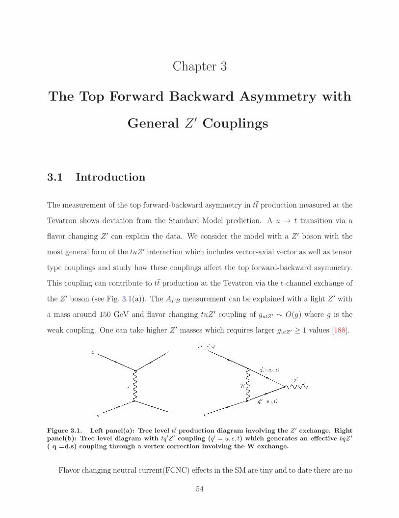
Chapter 3
The Top Forward Backward Asymmetry with
General Z ′ Couplings
3.1 Introduction
The measurement of the top forward-backward asymmetry in tt production measured at the
Tevatron shows deviation from the Standard Model prediction. A u → t transition via a
flavor changing Z ′ can explain the data. We consider the model with a Z ′ boson with the
most general form of the tuZ ′ interaction which includes vector-axial vector as well as tensor
type couplings and study how these couplings affect the top forward-backward asymmetry.
This coupling can contribute to tt production at the Tevatron via the t-channel exchange of
the Z ′ boson (see Fig. 3.1(a)). The AFB measurement can be explained with a light Z ′ with
a mass around 150 GeV and flavor changing tuZ ′ coupling of gutZ′ ∼ O(g) where g is the
weak coupling. One can take higher Z ′ masses which requires larger gutZ′ ≥ 1 values [188].
Figure 3.1. Left panel(a): Tree level tt production diagram involving the Z ′ exchange. Rightpanel(b): Tree level diagram with tq′Z ′ coupling (q′ = u, c, t) which generates an effective bqZ ′
( q =d,s) coupling through a vertex correction involving the W exchange.
Flavor changing neutral current(FCNC) effects in the SM are tiny and to date there are no
54
3.1 Introduction
experimental evidence of FCNC effects beyond those expected from the SM. There are some
anomalies in the B system which might require new physics to resolve but the NP generated
FCNC effects that are needed in the B system are much smaller than the one needed to
resolve the top AFB [189]. A tree level dbZ ′ or a sbZ ′ coupling is strongly suppressed by Bd,s
mixing. A tree level tq′Z ′ coupling, where q′ = u, c, t, will generate an effective bqZ ′(q = d, s)
coupling through a vertex correction involving the W exchange [190] (see Fig. 3.1(b)). The
Bq mixing constraints on these effective vertices would then lead to constraints on the tq′Z ′
coupling. The vertex corrections are divergent and can be regulated by a cut-off Λ which
represents the scale of NP in an effective theory framework. In NP models where there are
no bare bqZ ′ couplings the vertex corrections with a chosen Λ can be used to constrain the
tq′Z ′ coupling from Bq mixing measurements. We will take the scale of new physics to be
∼ TeV . In specific complete models Λ will represent the mass of some new particles. In
models of NP where there are bare bqZ ′ couplings the vertex correction will renormalize the
bare bqZ ′ vertices to produce the renormalized vertices Uqb. These renormalized vertices can
then be fitted to Bq mixing data. Assuming the vertex corrections to be less than or at
most the same size of the bare couplings one we can obtain bounds on the tqZ ′ couplings by
requiring the generated bqZ ′ coupling to be ≤ Uqb. It is possible to have models where large
bare bqZ ′ couplings cancel with large vertex corrections to produce small renormalized bqZ ′
vertices consistent with experiments. We will not consider these finely tuned model.
When the vertex corrections are computed one finds that right handed tuZ ′ couplings do
not contribute to Bq mixing in the limit of setting the up quark mass to zero. We note that
ttZ ′ couplings do not have such suppression and will contribute to Bq mixing via the vertex
corrections. Even though the ttZ ′ coupling does not contribute to the top AFB, in specific
models of NP this coupling may be related to the the FCNC coupling tuZ ′ [191]. It turns out
the Bq mixing constraints on ttZ ′ are weak because of the small CKM elements Vts(d) and
not because of right handed couplings. The tqZ ′(q = u, c, t) couplings via box diagrams can
55
3.2 Constraints on tq′(= u, t)Z ′ couplings from Bq(=d,s) mixing
produce an effective d(s)buu operator that can contribute to decays like B → K(K∗)π(η, η′ρ)
or B → π(ρ)π(ρ) e.t.c decays. The effects of these new operators can be observed in CP
violating and/or triple product measurements [192]. However these effective operators only
modify the SM Wilson’s co-efficients in the SM effective Hamiltonian and so the CP violating
predictions and /or triple product measurements should be similar to the SM for a reasonable
choice of tqZ ′(q = u, c, t) couplings.
We will next consider the most general tuZ ′ couplings including both vector, axial vec-
tor and tensor couplings( ∼ σµνqν
mt) and study the effect of these couplings on the top AFB.
The interesting feature about these tensor couplings are that we can avoid the Bq mixing
constraints due to the suppressions of these operators at low energies [193]. The momen-
tum dependence of these operators imply that at the b quark scale these operators will be
suppressed by ∼ mb/mt and consequently the Bq mixing constraints will be weak for these
operators.
In the next section we discuss the Bq(q = d, s) constraints on the tuZ ′ operators. In the
following section we introduce the general tuZ ′coupling including tensor terms and study
the effects in the top AFB. This is followed by the section on the t → uZ ′ branching ratio
calculations and, finally, summarize the results of this work.
3.2 Constraints on tq′(= u, t)Z ′ couplings from Bq(=d,s)
mixing
In general, new physics contributions to the mass difference between neutral Bq meson mass
eigenstates (∆Mq) can be constrained by the ∆Mq experimental results. In the SM, B0q -B
0q
mixing occurs at the one loop level by the flavor changing weak interaction box diagrams.
The mixing amplitude M q12 is related to the mass difference ∆Mq via ∆Mq = 2|M q
12|. The
56
3.2 Constraints on tq′(= u, t)Z ′ couplings from Bq(=d,s) mixing
recent theoretical estimations for the mass differences of B0s -B
0s and B0
d-B0d mixing [194] at
1σ confidence level(CL) are
(∆Ms)SM = 16.8+2.6
−1.5 ps−1 , (∆Md)
SM = 0.555+0.073−0.046 ps
−1. (3.1)
The latest measurements of mass difference by CDF [195] and DØ [196] for Bs mixing are
∆MBs = (17.77± 0.10(stat.)± 0.07(syst.)) ps−1
∆MBs = (18.53± 0.93(stat.)± 0.30(syst.)) ps−1 . (3.2)
The HFAG value for the mass difference ofB0d-B
0d mixing is ∆MBd
(exp) = (0.507±0.004) ps−1
[197]. The experimental results for the mass differences of both B0s -B
0s and B0
d-B0d mixing
are consistent with their SM expectations. Hence, the mass difference results can provide
strong constraints on NP contributions.
In this section we will consider the Bd,s mixing constraints on the tq′(= u, t)Z ′ couplings.
3.2.1 tuZ ′ left-handed coupling
The most general Lagrangian for flavor changing tuZ ′ transition is [198]
LtuZ′ = u[γµ(a+ bγ5) + i
σµνmt
qν(c+ dγ5)]tZ ′
µ , (3.3)
where q = pt−pu. In general the couplings a, b, c and d are complex and can be momentum
dependent (form factors). In this work we will take the couplings to be constants with
no momentum dependence. Consider the tuZ ′ vertex with a = −b = gLtu , and c=d=0
in Eq. (3.3). This generates effective bqZ ′(q = d, s) coupling at one loop level due to W
57
3.2 Constraints on tq′(= u, t)Z ′ couplings from Bq(=d,s) mixing
exchange. We obtain the bqZ ′ coupling in the Pauli-Villars regularization as
LZ′ = Uqbqγµ(1− γ5)bZ
′µ , (3.4)
where the contribution of the vertex correction in Fig. 3.1 is given by
δΓµ(p, p′) = g′∫
d4k
(2π)4u(p′)
(−gνρ + qνqρ/q2)γν(1− γ5)( 6k′ +mt)γ
µ(1− γ5) 6kγρ(1− γ5)
((p− k)2 −M2W + iε) (k′2 −m2
t + iε) (k2 + iε)u(p),
(3.5)
where
g′ = gLtu−iGF√
2M2
W (V ∗uqVtb + V ∗
tqVub), (3.6)
and leads to the effective coupling
Uqb = gLtuGF√2M2
W (V ∗uqVtb + V ∗
tqVub)1
8π2
[xtLog[ Λ2
m2t]− Log[ Λ2
M2W]
(xt − 1)
]. (3.7)
where Λ ∼ TeV is a cut-off scale, and xt = m2t/M
2W . The function Uqb includes only the
contribution from the W boson, and the contribution of the associated Goldston boson in
the SM is the order of mu/MW . Note that for Bd mixing the coupling gLtu is associated with
the CKM factor V ∗udVtb ∼ 1, and thus one can expect a strong constraint on gLtu from the
mass difference ∆Md.
A tree-level exchange of the Z ′ generates the ∆B = 2 effective Lagrangian responsible
for the neutral Bq meson mixing
H∆B=2Z′ =
U2qb
M2Z′
ηZ′(qb)V−A(qb)V−A , (3.8)
where (qb)V−A = qγµ(1 − γ5)b, and the QCD correction factor ηZ′ = [αs(MZ′)/αs(mb)]6/23.
The Z ′ contribution to the Bq mixing amplitude can be introduced in the matrix element
58
3.2 Constraints on tq′(= u, t)Z ′ couplings from Bq(=d,s) mixing
by using the vacuum insertion method as
MZ′ =U2qb
M2Z′
ηZ′〈B0q |(qγµ(1− γ5)b)
2|B0q 〉, (3.9)
where
〈B0q |(qγµ(1− γ5)b)
2|B0q 〉 =
∑
n
〈B0q |qγµ(1− γ5)b|n〉〈n|qγµ(1− γ5)b|B0
q 〉,
≡ BB〈B0q |qγµ(1− γ5)b|0〉〈0|qγµ(1− γ5)b|B0
q 〉,
= BB|〈0|qγµγ5b|B0q 〉|2,
=8
3BBf
2Bqm2
Bq, (3.10)
where BB is the bag factor and fBq is the decay constant. The mixing amplitude is given by
[M q12]
Z′
=|MZ′|2mBq
, (3.11)
where 1/2mBq is a normalization factor. Thus
[M q12]
Z′
=4
3
U2qb
M2Z′
ηZ′mBqf2BqBq. (3.12)
In the presence of new physics, the mixing amplitude M q12 can be parameterized by
complex parameters ∆q [194]
M q12 = [M q
12]SM,∆q. (3.13)
In our case, ∆q = |∆q|eiφ∆q = 1+ [M q
12]Z′
/[M q12]
SM . A global analysis on the parameters |∆q|
and φ∆q for Bd − Bd and Bs − Bs mixing are carried out in [194]. The best fit results for ∆d
59
3.2 Constraints on tq′(= u, t)Z ′ couplings from Bq(=d,s) mixing
and ∆s in this analysis at 1 σ CL ( scenario I) are
|∆d| = 0.747+0.195−0.082, φ∆
d = −12.9+3.8
−2.7 , (3.14)
and
|∆s| = 0.887+0.143−0.064, φ∆
s = −51.6+14.2
−9.7 or − 130.0+13
−12 . (3.15)
The ∆d constraint in Eq. (3.14) on the coupling gLtu at mt(mt) = (165.017±1.156±0.11)
GeV [194], βSM = 27.2+1.1
−3.1 [194], and MZ′ = 150 GeV is shown in Fig. 3.2. The numerical
values of all other theoretical inputs can be found in [194]. They are varied within 1 σ errors
in the fit. The cut-off scale Λ is varied between 300 GeV to 2 TeV . The green scatter points
in Fig. 3.2 satisfy only |∆d| in Eq. (3.14), while blue points satisfy both |∆d| and φ∆d in
Eq. (3.14). The results indicates that Bd mixing can strongly constrain the tuZ ′ coupling
gLtu even at Λ = 300 GeV. In particular we note that the maximum value for |gLtu| is around
0.2 and is associated with a large phase. In fact there are no real gLtu that satisfy the Bd
constraint.
On the other hand, Fig. 3.3 suggests that the constraints from Bs mixing on the tuZ ′
coupling gLtu are weaker (∼ O(1)) even at Λ = 2 TeV. This can be understood from the fact
that the Bs mixing contribution in this case is associated with the CKM factor V ∗usVtb and is
suppressed. The (green, blue, red) scatter points in Fig. 3.3 are constrained by ( |∆s|, (|∆s|
and φ∆s = −51.6+14.2
−9.7 ), (|∆s| and φ∆s = −130.0+13
−12 ) in Eq. (3.15). The large negative phase
φ∆s prefers large gLtu values.
60
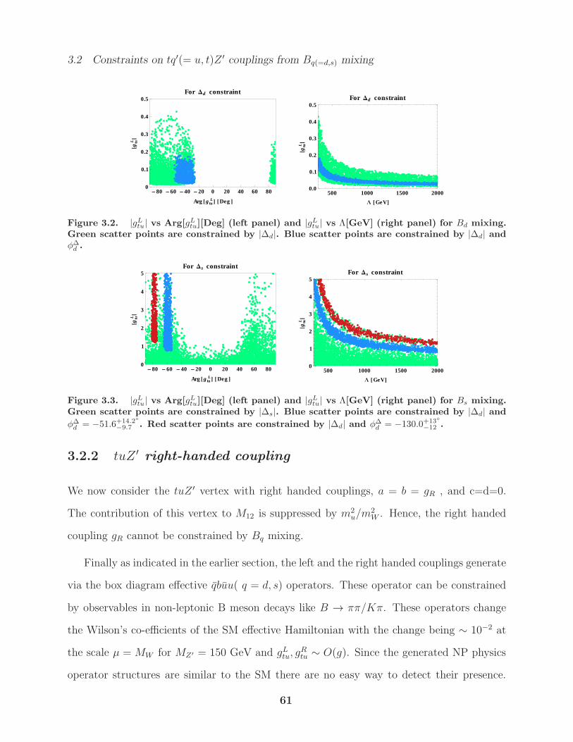
3.2 Constraints on tq′(= u, t)Z ′ couplings from Bq(=d,s) mixing
-80 -60 -40 -20 0 20 40 60 800
0.1
0.2
0.3
0.4
0.5
Arg @g tuLD @Deg D
ÈgtuLÈ
For Dd constraint
500 1000 1500 20000.0
0.1
0.2
0.3
0.4
0.5
L @GeVD
ÈgtuLÈ
For Dd constraint
Figure 3.2. |gLtu| vs Arg[gLtu][Deg] (left panel) and |gLtu| vs Λ[GeV] (right panel) for Bd mixing.Green scatter points are constrained by |∆d|. Blue scatter points are constrained by |∆d| andφ∆d.
-80 -60 -40 -20 0 20 40 60 800
1
2
3
4
5
Arg @g tuLD @Deg D
ÈgtuLÈ
For Ds constraint
500 1000 1500 20000
1
2
3
4
5
L @GeVD
ÈgtuLÈ
For Ds constraint
Figure 3.3. |gLtu| vs Arg[gLtu][Deg] (left panel) and |gLtu| vs Λ[GeV] (right panel) for Bs mixing.Green scatter points are constrained by |∆s|. Blue scatter points are constrained by |∆d| andφ∆d= −51.6+14.2
−9.7 . Red scatter points are constrained by |∆d| and φ∆d= −130.0+13
−12 .
3.2.2 tuZ ′ right-handed coupling
We now consider the tuZ ′ vertex with right handed couplings, a = b = gR , and c=d=0.
The contribution of this vertex to M12 is suppressed by m2u/m
2W . Hence, the right handed
coupling gR cannot be constrained by Bq mixing.
Finally as indicated in the earlier section, the left and the right handed couplings generate
via the box diagram effective qbuu( q = d, s) operators. These operator can be constrained
by observables in non-leptonic B meson decays like B → ππ/Kπ. These operators change
the Wilson’s co-efficients of the SM effective Hamiltonian with the change being ∼ 10−2 at
the scale µ = MW for MZ′ = 150 GeV and gLtu, gRtu ∼ O(g). Since the generated NP physics
operator structures are similar to the SM there are no easy way to detect their presence.
61
3.2 Constraints on tq′(= u, t)Z ′ couplings from Bq(=d,s) mixing
A detailed fit to all the non-leptonic data may provide constraints on the couplings gL,Rtu ,
which we do not perform in this work. Some analysis along this line has been done for tdW ′
coupling in [199].
3.2.3 ttZ ′ coupling
For completeness, next we consider Bq mixing constraints on the ttZ ′ couplings. The La-
grangian for the ttZ ′ interaction is
LttZ′ = t[gLttγµ(1− γ5) + gRttγ
µ(1 + γ5)]tZ′µ. (3.16)
Again, we evaluate the one-loop diagram (see Fig. 3.1(b)) in the Pauli-Villars regularization
and obtain the effective Lagrangian for bq(=d,s)Z ′ interaction as
L′Z′ = U ′
qbqγµ(1− γ5)bZ
′µ , (3.17)
where
U ′qb =
GF√2M2
WVtqVtbftt(Λ, xt) , (3.18)
with
ftt(Λ, xt) =1
(4π2)
∫ 1
0
dx
∫ 1−y
0
dy[gLtt
(Log[
xΛ2
M2WDtt
] +1
2
x2tDtt
)+ gRttxt
(12Log[
xΛ2
M2WDtt
] +1
Dtt
)],
(3.19)
62
3.3 Top quark forward-backward asymmetry
and Dtt = x + (1 − x)xt. The function ftt includes both the W boson and the associated
Goldston boson contributions. The ttZ ′ contribution to the Bq mixing amplitude is
[M q12]
Z′
=4
3
[U ′qb]
2
M2Z′
ηZ′mBqf2BqBq. (3.20)
Both Bd − Bd and Bs − Bs constraints in Eqs. (3.14) and (3.15) can allow large ∼ O(1)
values for gL,Rtt .
3.3 Top quark forward-backward asymmetry
In this section we calculate the top AFB keeping in mind the constraints derived on the
coupling from the previous section. The most general Lagrangian for a flavor changing tuZ ′
interaction is given in Eq. (3.3). This interaction can contribute to uu → tt scattering
amplitude through the t-channel exchange of the Z ′ boson (see Fig. 3.1(a)). The SM and Z ′
matrix elements are
MSM =g2s(t
a)ji(ta)lk
s
(vuj
(p2)γµuui
(p1))(utl(p3)γµvtk(p4)) ,
MZ′ =1
t−M2Z′ + iMZ′ΓZ′[
utl(p3)
(γµ(a + bγ5) + i
σµνmt
qν(c+ dγ5)
)uui
(p1)
](−gµα + qµqα/q2)
[vuj
(p2)
(γα(a+ bγ5) + i
σαβmt
qβ(c+ dγ5)
)vtk(p4)
]. (3.21)
The tree-level differential cross section for qq → tt process in the tt c.m. frame including
both the SM and for Z ′ contributions is
dσ
d cos θ=
βt32πs
(ASM +ASM−Z′ +AZ′) , (3.22)
63
3.3 Top quark forward-backward asymmetry
where s = (pq + pq)2 is the squared c.m. energy of the tt system, βt =
√1− 4m2
t/s, and the
polar angle θ is the relative angle between direction of motion of the outgoing top-quark and
the incoming q-quark. The quantities ASM , ASM−Z′, and AZ′ denote the leading order SM,
the interference between the SM and Z ′, and the pure Z ′ scattering amplitudes, respectively.
These amplitudes can be obtained in terms of kinematic variables θ and s as
ASM =2g4s9
[1 + c2θ +
4m2t
s
],
ASM−Z′ =2g2s9
[ t−M2Z′
(t−M2Z′)2 +M2
Z′Γ2Z′
](f1 + f2) ,
AZ′ =1
4
[ 1
(t−M2Z′)2 +M2
Z′Γ2Z′
](f3 + f4 + f5). (3.23)
Where cθ = βt cos θ, and t = (pq−pt)2 = −s/2(1−βt cos θ)+m2t . The functions fis (i = 1..5)
can be found in Appendix. B. Here we assume the couplings a, b, c and d to be real. Our
results for tt production are obtained by the convolution of the analytic differential cross
section of Eq. (3.22) with the CTEQ-5L parton distribution functions [200] implemented
in Mathematica. We expect the MSTW 2008 [201] parton distributions to give compatible
results.
The forward-backward asymmetry of the top quark in the tt c.m. frame is defined as
[202]
AttFB =
σF − σBσF + σB
, (3.24)
where
σF =
∫ 1
0
dσ
d cos θd cos θ , σB =
∫ 0
−1
dσ
d cos θd cos θ. (3.25)
In our analysis, we choose some representative values for the couplings a, b, c, and d to
64
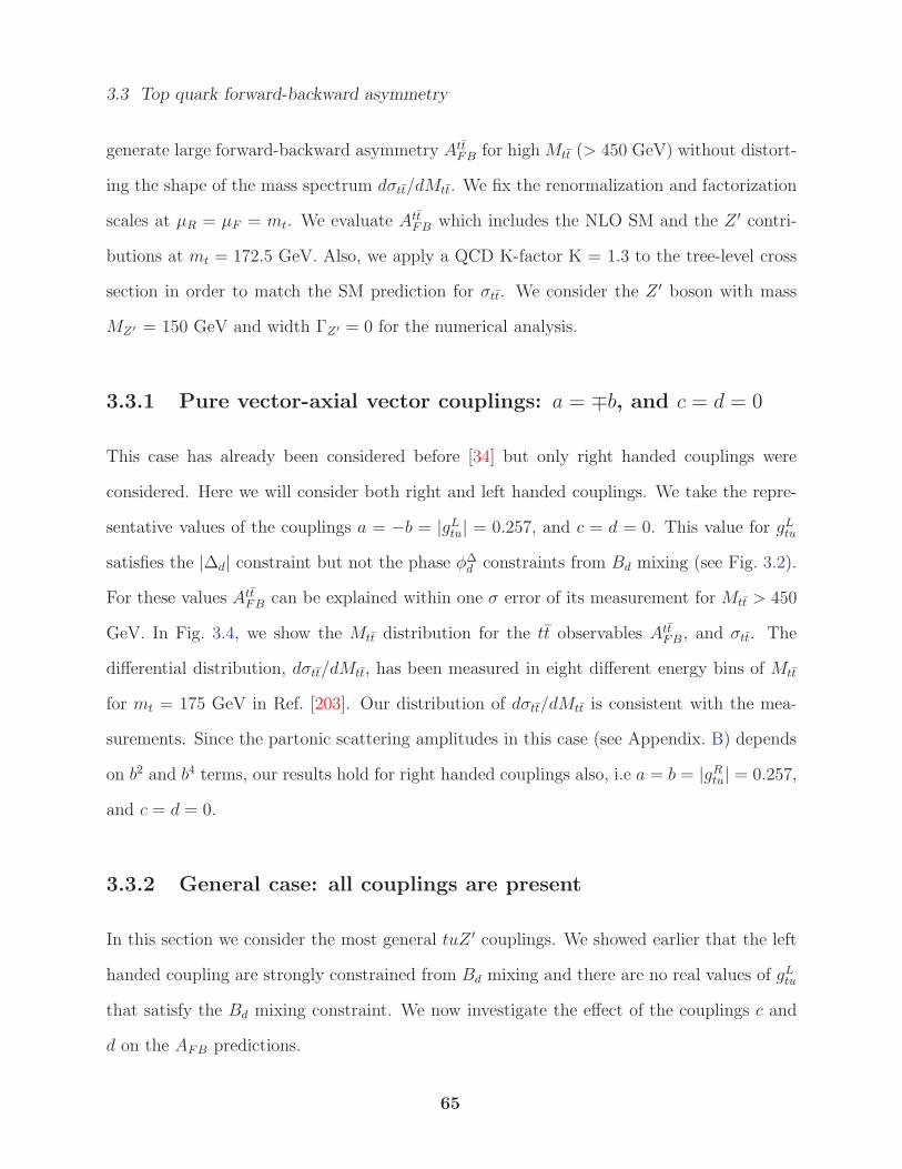
3.3 Top quark forward-backward asymmetry
generate large forward-backward asymmetry AttFB for highMtt (> 450 GeV) without distort-
ing the shape of the mass spectrum dσtt/dMtt. We fix the renormalization and factorization
scales at µR = µF = mt. We evaluate AttFB which includes the NLO SM and the Z ′ contri-
butions at mt = 172.5 GeV. Also, we apply a QCD K-factor K = 1.3 to the tree-level cross
section in order to match the SM prediction for σtt. We consider the Z ′ boson with mass
MZ′ = 150 GeV and width ΓZ′ = 0 for the numerical analysis.
3.3.1 Pure vector-axial vector couplings: a = ∓b, and c = d = 0
This case has already been considered before [34] but only right handed couplings were
considered. Here we will consider both right and left handed couplings. We take the repre-
sentative values of the couplings a = −b = |gLtu| = 0.257, and c = d = 0. This value for gLtu
satisfies the |∆d| constraint but not the phase φ∆d constraints from Bd mixing (see Fig. 3.2).
For these values AttFB can be explained within one σ error of its measurement for Mtt > 450
GeV. In Fig. 3.4, we show the Mtt distribution for the tt observables AttFB, and σtt. The
differential distribution, dσtt/dMtt, has been measured in eight different energy bins of Mtt
for mt = 175 GeV in Ref. [203]. Our distribution of dσtt/dMtt is consistent with the mea-
surements. Since the partonic scattering amplitudes in this case (see Appendix. B) depends
on b2 and b4 terms, our results hold for right handed couplings also, i.e a = b = |gRtu| = 0.257,
and c = d = 0.
3.3.2 General case: all couplings are present
In this section we consider the most general tuZ ′ couplings. We showed earlier that the left
handed coupling are strongly constrained from Bd mixing and there are no real values of gLtu
that satisfy the Bd mixing constraint. We now investigate the effect of the couplings c and
d on the AFB predictions.
65
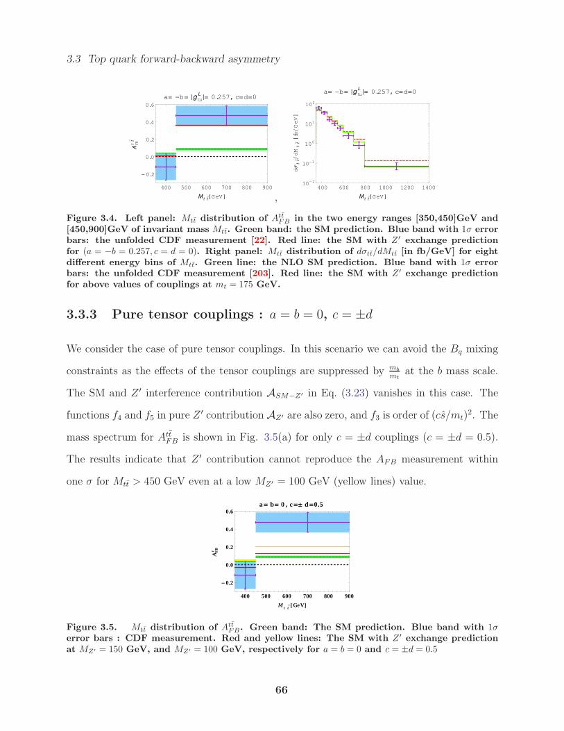
3.3 Top quark forward-backward asymmetry
400 500 600 700 800 900
- 0.2
0.0
0.2
0.4
0.6
M t t @GeV D
AFBtt
a= -b= Ègtu
LÈ= 0.257, c=d=0
,400 600 800 1000 1200 1400
10-2
10-1
100
101
102
M t t @GeV D
dΣ
ttdM
tt@fbGeVD
a= -b= Ègtu
LÈ= 0.257, c=d=0
Figure 3.4. Left panel: Mtt distribution of AttFB
in the two energy ranges [350,450]GeV and[450,900]GeV of invariant mass Mtt. Green band: the SM prediction. Blue band with 1σ errorbars: the unfolded CDF measurement [22]. Red line: the SM with Z ′ exchange predictionfor (a = −b = 0.257, c = d = 0). Right panel: Mtt distribution of dσtt/dMtt [in fb/GeV] for eightdifferent energy bins of Mtt. Green line: the NLO SM prediction. Blue band with 1σ errorbars: the unfolded CDF measurement [203]. Red line: the SM with Z ′ exchange predictionfor above values of couplings at mt = 175 GeV.
3.3.3 Pure tensor couplings : a = b = 0, c = ±d
We consider the case of pure tensor couplings. In this scenario we can avoid the Bq mixing
constraints as the effects of the tensor couplings are suppressed by mb
mtat the b mass scale.
The SM and Z ′ interference contribution ASM−Z′ in Eq. (3.23) vanishes in this case. The
functions f4 and f5 in pure Z ′ contribution AZ′ are also zero, and f3 is order of (cs/mt)2. The
mass spectrum for AttFB is shown in Fig. 3.5(a) for only c = ±d couplings (c = ±d = 0.5).
The results indicate that Z ′ contribution cannot reproduce the AFB measurement within
one σ for Mtt > 450 GeV even at a low MZ′ = 100 GeV (yellow lines) value.
400 500 600 700 800 900
-0.2
0.0
0.2
0.4
0.6
M t t @GeVD
AFBt
a= b= 0 , c=± d=0.5
Figure 3.5. Mtt distribution of AttFB
. Green band: The SM prediction. Blue band with 1σerror bars : CDF measurement. Red and yellow lines: The SM with Z ′ exchange predictionat MZ′ = 150 GeV, and MZ′ = 100 GeV, respectively for a = b = 0 and c = ±d = 0.5
66
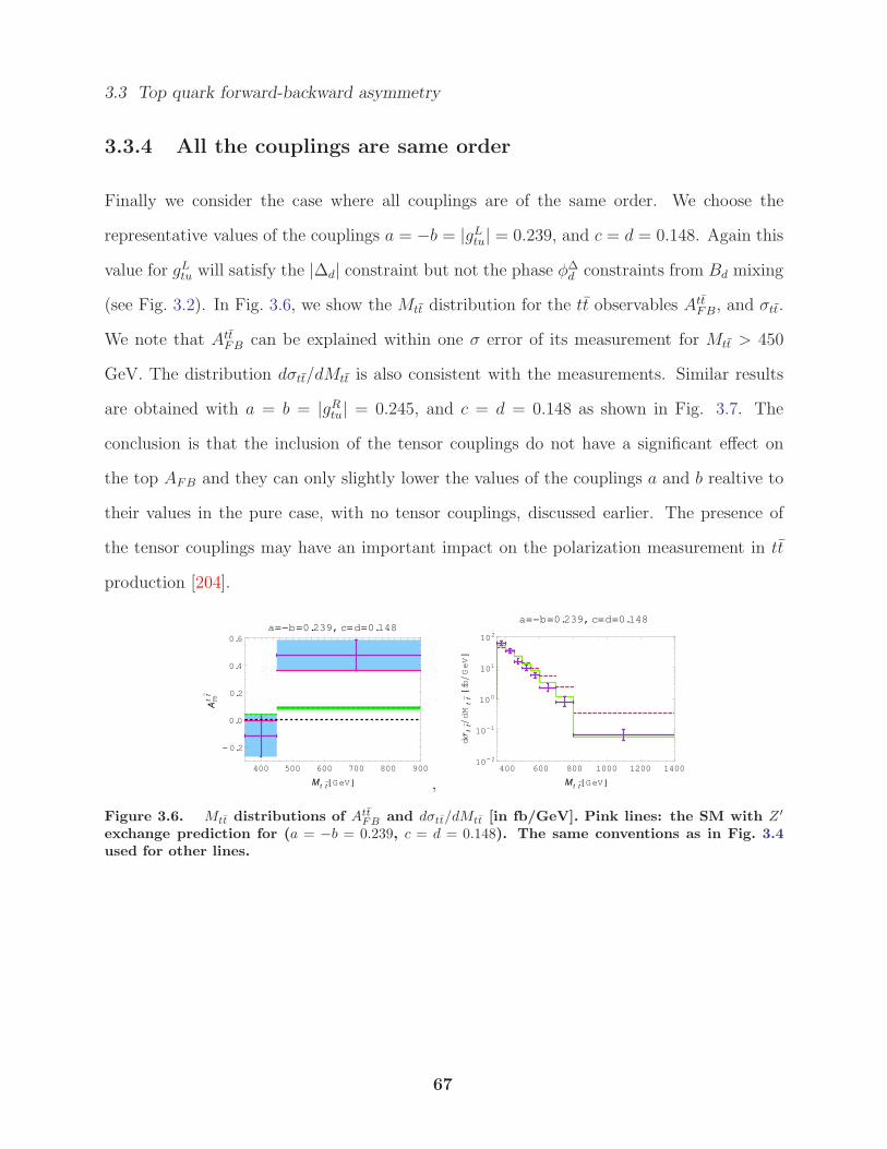
3.3 Top quark forward-backward asymmetry
3.3.4 All the couplings are same order
Finally we consider the case where all couplings are of the same order. We choose the
representative values of the couplings a = −b = |gLtu| = 0.239, and c = d = 0.148. Again this
value for gLtu will satisfy the |∆d| constraint but not the phase φ∆d constraints from Bd mixing
(see Fig. 3.2). In Fig. 3.6, we show the Mtt distribution for the tt observables AttFB, and σtt.
We note that AttFB can be explained within one σ error of its measurement for Mtt > 450
GeV. The distribution dσtt/dMtt is also consistent with the measurements. Similar results
are obtained with a = b = |gRtu| = 0.245, and c = d = 0.148 as shown in Fig. 3.7. The
conclusion is that the inclusion of the tensor couplings do not have a significant effect on
the top AFB and they can only slightly lower the values of the couplings a and b realtive to
their values in the pure case, with no tensor couplings, discussed earlier. The presence of
the tensor couplings may have an important impact on the polarization measurement in tt
production [204].
400 500 600 700 800 900
- 0.2
0.0
0.2
0.4
0.6
M t t @GeV D
AFBtt
a=-b=0.239, c=d=0.148
,400 600 800 1000 1200 1400
10-2
10-1
100
101
102
M t t @GeV D
dΣ
ttdM
tt@fbGeVD
a=-b=0.239, c=d=0.148
Figure 3.6. Mtt distributions of AttFB
and dσtt/dMtt [in fb/GeV]. Pink lines: the SM with Z ′
exchange prediction for (a = −b = 0.239, c = d = 0.148). The same conventions as in Fig. 3.4used for other lines.
67
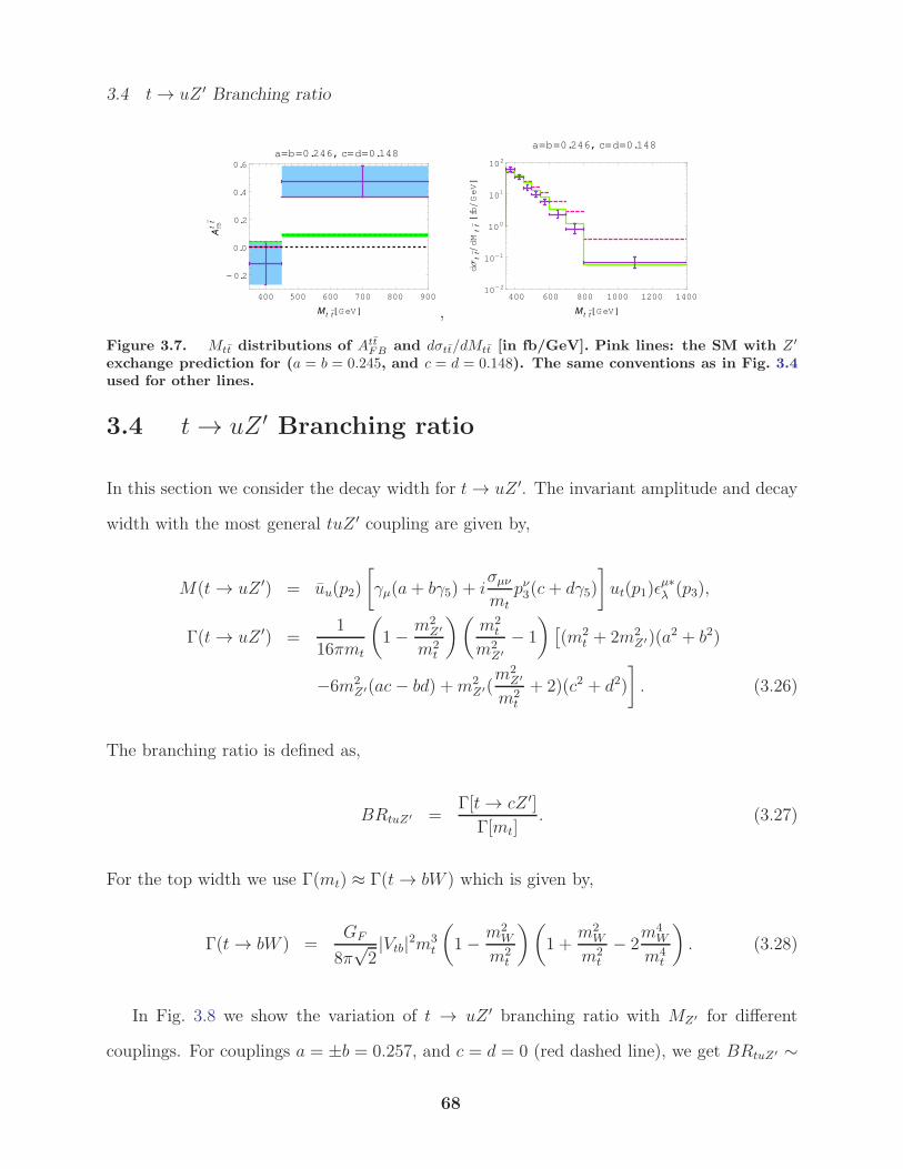
3.4 t→ uZ ′ Branching ratio
400 500 600 700 800 900
- 0.2
0.0
0.2
0.4
0.6
M t t @GeV D
AFBtt
a=b=0.246, c=d=0.148
,400 600 800 1000 1200 1400
10-2
10-1
100
101
102
M t t @GeV D
dΣ
ttdM
tt@fbGeVD
a=b=0.246, c=d=0.148
Figure 3.7. Mtt distributions of AttFB
and dσtt/dMtt [in fb/GeV]. Pink lines: the SM with Z ′
exchange prediction for (a = b = 0.245, and c = d = 0.148). The same conventions as in Fig. 3.4used for other lines.
3.4 t→ uZ ′ Branching ratio
In this section we consider the decay width for t→ uZ ′. The invariant amplitude and decay
width with the most general tuZ ′ coupling are given by,
M(t → uZ ′) = uu(p2)
[γµ(a+ bγ5) + i
σµνmt
pν3(c+ dγ5)
]ut(p1)ǫ
µ∗λ (p3),
Γ(t→ uZ ′) =1
16πmt
(1− m2
Z′
m2t
)(m2
t
m2Z′
− 1
)[(m2
t + 2m2Z′)(a2 + b2)
−6m2Z′(ac− bd) +m2
Z′(m2
Z′
m2t
+ 2)(c2 + d2)
]. (3.26)
The branching ratio is defined as,
BRtuZ′ =Γ[t→ cZ ′]
Γ[mt]. (3.27)
For the top width we use Γ(mt) ≈ Γ(t→ bW ) which is given by,
Γ(t→ bW ) =GF
8π√2|Vtb|2m3
t
(1− m2
W
m2t
)(1 +
m2W
m2t
− 2m4
W
m4t
). (3.28)
In Fig. 3.8 we show the variation of t → uZ ′ branching ratio with MZ′ for different
couplings. For couplings a = ±b = 0.257, and c = d = 0 (red dashed line), we get BRtuZ′ ∼
68
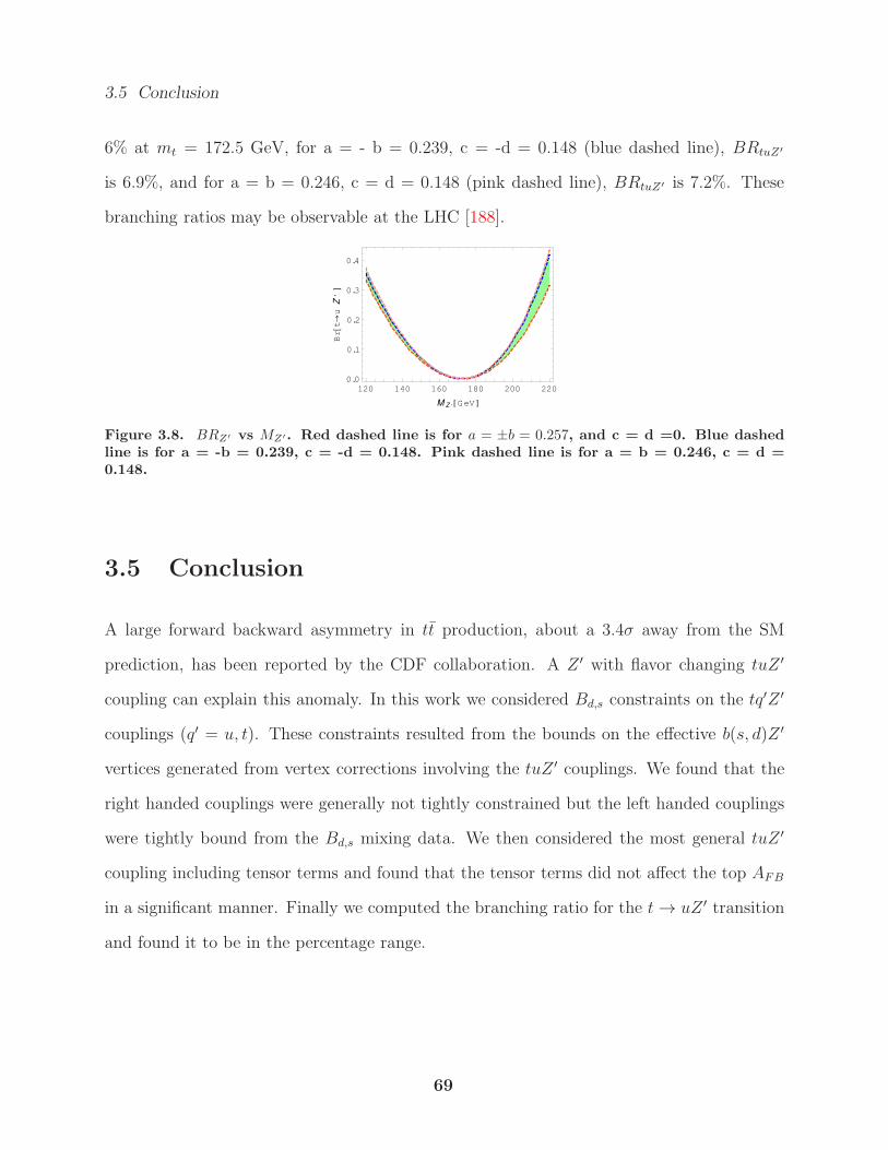
3.5 Conclusion
6% at mt = 172.5 GeV, for a = - b = 0.239, c = -d = 0.148 (blue dashed line), BRtuZ′
is 6.9%, and for a = b = 0.246, c = d = 0.148 (pink dashed line), BRtuZ′ is 7.2%. These
branching ratios may be observable at the LHC [188].
120 140 160 180 200 220
0.0
0.1
0.2
0.3
0.4
M Z ,@GeV D
Br@t®u
Z,D
Figure 3.8. BRZ′ vs MZ′. Red dashed line is for a = ±b = 0.257, and c = d =0. Blue dashedline is for a = -b = 0.239, c = -d = 0.148. Pink dashed line is for a = b = 0.246, c = d =0.148.
3.5 Conclusion
A large forward backward asymmetry in tt production, about a 3.4σ away from the SM
prediction, has been reported by the CDF collaboration. A Z ′ with flavor changing tuZ ′
coupling can explain this anomaly. In this work we considered Bd,s constraints on the tq′Z ′
couplings (q′ = u, t). These constraints resulted from the bounds on the effective b(s, d)Z ′
vertices generated from vertex corrections involving the tuZ ′ couplings. We found that the
right handed couplings were generally not tightly constrained but the left handed couplings
were tightly bound from the Bd,s mixing data. We then considered the most general tuZ ′
coupling including tensor terms and found that the tensor terms did not affect the top AFB
in a significant manner. Finally we computed the branching ratio for the t→ uZ ′ transition
and found it to be in the percentage range.
69
Chapter 4
The Charged Lepton Mass Matrix and
Non-zero θ13 with TeV Scale New Physics
4.1 Introduction
The leptonic mixing arises from the overlap of matrices that diagonalize the charged lepton
and the neutrino mass matrices. Many approaches to studying the leptonic mixing start in
the basis where the charged lepton mass is diagonal. Our approach to obtaining the leading
order leptonic mixing as well as deviations from it starts from the charged lepton sector. A
recent attempt to understand θ13 from the charged lepton sector can be found in Ref. [48] and
in the past corrections to the leptonic mixing from the charged lepton sector were considered
in Ref. [205]. An approach to suppress flavor changing neutral current effects (FCNC) in the
quark sector, based on shared flavor symmetry, was proposed in Ref. [206]. As an example of
this shared symmetry the decoupled 2− 3 symmetry was used for the down quark sector to
suppress FCNC effects and explain anomalies [207] observed in the B meson system. In the
decoupled limit the first generation is decoupled from the other two generations. We extend
this decoupled 2− 3 symmetry to the charged lepton sector. This is a reasonable extension
given the fact that the down quark and charged leptons exhibit similar hierarchical structure
and they may be combined in representations of GUT groups.
One of the central ideas of this approach is the requirement that the mass matrices, in a
symmetric limit, be diagonalized by unitary matrices composed of pure numbers independent
of the parameters of the mass matrices. This is similar to the idea of form diagonalizable
matrices discussed in Ref. [208]. If one starts with a 2 − 3 symmetric mass matrix for the
70
4.1 Introduction
charged lepton sector and requires it to be diagonalized by unitary matrices of pure numbers
one recovers the decoupled 2 − 3 symmetry. In the neutrino sector we assume the third
generation to be decoupled from the first two generations. With real entries in the neutrino
mass matrix it is diagonalized by a rotation matrix and the resulting leptonic mixing has a
µ−τ symmetry. Requiring the mass matrix to be diagonalized by pure numbers can lead to,
among other structures, the BM and the TBM leptonic mixing depending on the structure
of the chosen mass matrix.
In the bimaximal case, to generate the mixing matrices in the charged lepton and the
neutrino sector, we present a Lagrangian that extends the SM by three right handed neu-
trinos, an additional Higgs doublet and two singlet scalar fields.1 The Lagrangian uses the
same class of Z2 symmetries as has been used in Ref [210]. However, the structure as well
as the phenomenology of our model is very different from the above mentioned papers. The
Lagrangian is constructed to have a 2 − 3 symmetry, Z232 , along with two additional Z2
symmetries Ze2 and ZD
2 . The neutrino masses and mixing are generated through the usual
see-saw mechanism. The presence of the Z232 × Ze
2 symmetries leads to the decoupled 2− 3
symmetry in the charged lepton sector and fixes the interactions of the right handed neu-
trinos with the singlet scalar fields. The presence of the ZD2 symmetry forces the neutrinos
to acquire Dirac masses by coupling to a second Higgs doublet which has a different ZD2
transformation than the usual SM Higgs doublet that give masses to the charged leptons.
The full Lagrangian is symmetric under the product of the Z2 symmetries, Z232 × Ze
2 × ZD2 .
In tri-bimaximal case, we introduce a Lagrangian that extends the SM particle content
by three right-handed neutrinos, three complex singlet scalar fields, and an additional Higgs
doublet. The symmetry group of the SM is extended by the product of the symmetries
Z4×U(1). The Z4 symmetry serves to have a 2−3 symmetric Yukawa matrix in the charged
lepton sector and yields the mass matrices in the charged lepton and neutrino sector to have
1Recent motivations for considering two Higgs doublet models can be found in Ref. [209].
71
4.1 Introduction
decoupled structures. We present a global U(1) symmetry which equates certain couplings
of the charged leptons and neutrinos as we relate the couplings to the U(1) charges. The
U(1) symmetry forbids the Majorana masses of the right-handed neutrinos. The Majorana
neutrino masses are generated via the v.e.v of the singlet scalars and the U(1) gets broken
spontaneously. Without altering the lepton mixing, an additional Majorana mass term is
introduced to protect one of the neutrino masses from blowing up.
The neutrino masses and mixing arise when the Higgs doublets and the singlet scalars
acquire v.e.v’s and break the symmetries of the Lagrangian. The leptonic mixing is predicted
to be either of bimaximal or tri-bimaximal type when the singlet scalars acquire the same
v.e.v. If the v.e.v of the second Higgs doublet is small enough ∼MeV then the see-saw scale
as well as the masses of the singlet scalars can be in the TeV range.
Symmetry breaking in both cases is introduced in the charged lepton sector by higher
dimensional operators that break the decoupled 2−3 symmetry but generate a 2−3 symmet-
ric mass matrix except for a single breaking generated by the muon mass. In the neutrino
sector, symmetry breaking is introduced by breaking the alignment of the v.e.v’s of the sin-
glet scalars by terms in the effective potential. The corrections to leptonic mixing go as
∼ v2
ω2 where v is the v.e.v of the SM Higgs and ω the scale of the singlet scalar v.e.v’s. If
ω ∼ TeV then the corrections to the leptonic mixing are enough to explain the experimental
observations.
broken spontaneously. Without altering the lepton mixing, an additional Majorana mass
term is introduced to protect one of the neutrino masses from blowing up.
Here, we begin with studying the flavor symmetric limit in the lepton sector that leads
to the BM and TBM mixing. In the following two sections we present the Lagrangians that
are invariant under the underlying symmetry groups in both the BM and TBM cases, and
study the effects of symmetry breaking in the charged lepton and neutrino sector to generate
the realistic leptonic mixing matrix. Finally, we show the numerical results in each case and
72
4.2 The leptonic mixing in the symmetric limit
summarize the results.
4.2 The leptonic mixing in the symmetric limit
We start with the charged lepton sector, and assume that the Yukawa matrix is 2 − 3
symmetric [211]. The Yukawa couplings of the charged leptons are given by
Y L =
l11 l12 −l12l12 l22 l23
−l12 l23 l22
. (4.1)
The above Yukawa matrix can be diagonalized as
U †Y LU = Y Ldiag,
U =
1 0 0
0 1√2
1√2
0 − 1√2
1√2
·
cos θ sin θ 0
− sin θ cos θ 0
0 0 1
, (4.2)
where the mixing angle θ is determined by the positive solution to
tan θ =2√2l12
l22 − l23 − l11 ±√
(l22 − l23 − l11)2 + 8l212. (4.3)
The eigenvalues of Y L are 12[l11+ l22− l23±
√(l11 − l22 + l23)2 + 8l212] and l22+ l23. According
to our assumption, the elements of the matrix that diagonalizes Y L must be pure numbers
in the symmetric limit. It is clear that we can achieve that by setting l12 = 0 (θ = 0) in
Eq. 4.3. This generates the decoupled 2-3 symmetry [206], as the flavor symmetry in the
charged lepton sector in which the first generation is decoupled from the second and third
generations.
73
4.2 The leptonic mixing in the symmetric limit
One can represent the Yukawa matrix with the decoupled 2-3 symmetry by Y L23 as
Y L23 =
l11 0 0
0 12l22
12l23
0 12l23
12l22
. (4.4)
This Yukawa matrix Y L23 is diagonalized by the unitary matrix W l
23 given by
W l23 =
1 0 0
0 − 1√2
1√2
0 1√2
1√2
. (4.5)
Note that this matrix differs from the one in Eq. 4.2 in the limit θ = 0 by an irrelevant
diagonal phase matrix. Writing the diagonalized Yukawa matrix as Y L23d we have
Y L23d = W l†
23YL23W
l23 =
l11 0 0
0 12(l22 − l23) 0
0 0 12(l22 + l23)
. (4.6)
The charged lepton masses are given by
me = ± v1√2l11,
mµ = ± v1√2
(l22 − l23)
2,
mτ = ± v1√2
(l22 + l23)
2. (4.7)
Since mµ << mτ there has to be a fine tuned cancellation between l22 and l23 to produce the
muon mass. Hence, it is more natural to consider the symmetry limit l22 = l23 which leads
74
4.2 The leptonic mixing in the symmetric limit
to mµ = 0. The Yukawa matrix which leads to the zero muon mass within the decoupled
2-3 symmetry is
Y L23 =
l11 0 0
0 12lT
12lT
0 12lT
12lT
. (4.8)
In the neutrino sector we assume that, in the symmetric limit, Mν has the general
structure
Mν =
a d 0
d b 0
0 0 c
, (4.9)
where all the parameters are real. This can be diagonalized by the matrix
W ν12 =
c12 s12 0
s12 −c12 0
0 0 1
,
s12 ≡ sin θ12, c12 ≡ cos θ12, (4.10)
where
tan 2θ12 =2d
(a− b). (4.11)
We can then calculate UsPMNS as
UsPMNS = U †
ℓUν , (4.12)
75
4.2 The leptonic mixing in the symmetric limit
with
Uℓ = W l23,
Uν = W ν12, (4.13)
where W l23 and W ν
23 are given in Eq. 4.5 and in Eq. 4.10.
This gives
UsPMNS =
c12 s12 0
− 1√2s12
1√2c12
1√2
1√2s12 − 1√
2c12
1√2
, (4.14)
which is just the µ − τ symmetric leptonic mixing. If we require θ12 in Eq. 4.11 to be
independent of the parameters a, b and d, then, we either have a = b which leads to
θ12 = π/4 and generates the BM mixing
Mν =
a d 0
d a 0
0 0 c
. (4.15)
with mass eigenvalues
Mdν = diag (a+ d, a− d, c). (4.16)
or d = k(a−b) and in particular we obtain the tri-bimaximal mixing with sin θ12 =1√3where
k =√2 and
Mν =
a√2(a− b) 0
√2(a− b) b 0
0 0 c
. (4.17)
76
4.3 Bimaximal mixing
The mass eigenvalues are given by
Mdν = diag (2a− b, 2b− a, c). (4.18)
We see that the neutrino mass matrix exhibits decoupling of the first two generations from
the third one. We will study both cases here in this work.
4.3 Bimaximal mixing
In this section, we use the bimaximal structure as the mixing matrix in the flavor symmetric
limit. We present the Lagrangian required to generate the BM pattern. Finally, we study
the effect of breaking the flavor symmetry on both sectors and show the numerical results.
4.3.1 The Lagrangian in the symmetric limit
Here, we present a simple Lagrangian that generates the mixing matrices considered in the
previous section. We find that the model naturally generates the BM mixing though the
TBM mixing can also be obtained but with introducing different flavor symmetries. Our
phenomenology will be done in the scenario in which the leptonic mixing is BM in the
symmetric limit.
We will use the seesaw mechanism to obtain the neutrino masses. Our model extends
the SM by an additional Higgs doublet and two singlet scalars. The particle content of the
model is given as
• three left-handed lepton doublets DαL, where α denotes e, µ, and τ ,
• three right-handed charged-lepton singlet αR, and
• three right-handed neutrino singlets ναR.
77
4.3 Bimaximal mixing
In the scalar sector, we employ
• two Higgs doublets φj with vacuum expectation values, v.e.v,⟨0|φ0
j |0⟩=
vj√2and
• two real singlet scalar fields ǫ1 and ǫ2, with v.e.v’s 〈0|ǫ0k|0〉 = wk.
The symmetries of the Lagrangian are introduced as
Z232 : DµL
↔ −DτL , µR ↔ −τR, νµR ↔ −ντR,
DeL → DeL, eR → eR, νeR → νeR,
ǫ1 → −ǫ1, ǫ2 → ǫ2, φ1 → φ1, φ2 → φ2,
Ze2 : νeR, eR, DeL, ǫ1, ǫ2, (Change sign, and the rest of the fields remain same)
ZD2 : νeR, νµR, ντR, φ2, (Change sign, and the rest of the fields remain same).
(4.19)
The most general Lagrangian consistent with the symmetries is
LY = y1DeLeRφ1 + y2(DµL
µR + DτLτR)φ1 + y3
(DµL
τR + DτLµR
)φ1
+[y4DeLνeR + y5
(DµL
νµR + DτLντR)]φ2 + h.c., (4.20)
LM =1
2
[MνTeRC
−1νeR +MPνTµRC
−1νµR +MPνTτRC
−1ντR]
− 1
2yνTeRC
−1
(νµR
(aǫ1 + bǫ2)√2
+ ντR(aǫ1 − bǫ2)√
2
)+ h.c. (4.21)
Here, φi ≡ iσ2φ∗i is the conjugate Higgs doublet and we have chosen to work in a basis where
the Dirac mass matrix for the neutrinos is diagonal. We can simplify the Lagrangian in
several ways. First, we can redefine aǫ1 → ǫ1 and bǫ2 → ǫ2. Second, to reduce the number of
parameters we can impose an approximate symmetry of the Lagrangian. A SU(3) symmetry
78
4.3 Bimaximal mixing
where the right handed singlet fields and the left handed doublet fields transform as the SU(3)
triplets leads to y4 = y5 = yD. The SU(3) symmetry is only satisfied by the Dirac mass
term for the neutrinos and is broken by the other terms in the Lagrangian. Third, we will
require the Lagrangian to be invariant under the transformation of the right-handed charged
leptons (µR ↔ −τR, eR → −eR, φ1 → −φ1), with all other fields remaining unchanged. This
symmetry requires y2 = y3 leading to vanishing µ mass. The µ mass is introduced later as a
symmetry breaking term. Finally, we will set the Majorana mass terms M = MP . We can
then rewrite the Lagrangian as
LY = y1DeLeRφ1 + y2(DµL
µR + DτLτR)φ1 + y2
(DµL
τR + DτLµR
)φ1
+ yD[DeLνeR + DµL
νµR + DτLντR]φ2 + h.c., (4.22)
LM =1
2M
[νTeRC
−1νeR + νTµRC−1νµR + νTτRC
−1ντR]
− 1
2yνTeRC
−1
(νµR
(ǫ1 + ǫ2)√2
+ ντR(ǫ1 − ǫ2)√
2
)+ h.c. (4.23)
The most general scalar potential V that is invariant under Z232 × Ze
2 × ZD2 is given by
V = −µ21ǫ
21 − µ2
2ǫ22 + λ1ǫ
41 + λ2ǫ
42 + λ′1ǫ
21ǫ
22
+ σ1ǫ21|φ1|2 + σ2ǫ
21|φ2|2 + σ3ǫ
22|φ1|2 + σ4ǫ
22|φ2|2 + V2HD(φ1, φ2), (4.24)
where V2HD(φ1, φ2) is the potential of the two Higgs doublets,
V2HD(φ1, φ2) = −µ2φ1φ†1φ1 − µ2
φ2φ†2φ2 + λφ1
(φ†1φ1)
2 + λφ2(φ†
2φ2)2 + λφ12
(φ†1φ1 + φ†
2φ2
)2
+ λ′φ12
(φ†1φ1 − φ†
2φ2
)2
+ λφ21
((φ†
1φ1)(φ†2φ2)− (φ†
1φ2)(φ†2φ1)
)
+ λ′φ21
((φ†
1φ1)(φ†2φ2) + (φ†
1φ2)(φ†2φ1)
). (4.25)
79
4.3 Bimaximal mixing
If we impose an additional symmetry to the above potential such as ǫ1 ↔ ǫ2, then the
potential takes the form
V = −µ2(ǫ21 + ǫ22
)+(ǫ21 + ǫ22
) 2∑
i=1
σiφ†iφi + λ
(ǫ21 + ǫ22
)2
+ λ′(ǫ21 − ǫ22
)2+ V2HD(φ1, φ2). (4.26)
We can parametrize the v.e.v’s of the singlet scalars as follows
〈0 |ǫ1| 0〉 = w cos γ and 〈0 |ǫ2| 0〉 = w sin γ. (4.27)
Thus, the only term that depends on γ is
f(γ) ≡ λ′w4 cos2 2γ. (4.28)
By minimizing f(γ), one gets
cos 2γ = 0. (4.29)
Thus
〈0 |ǫ1| 0〉 = 〈0 |ǫ2| 0〉 =w√2. (4.30)
By minimizing the above potential one can find the parameter w and the v.e.v’s of the two
Higgs doublets which are nonzero and different in the symmetric limit
v1 =
√α1
2β1,
v2 =
√α2
2β2, (4.31)
80
4.3 Bimaximal mixing
where
α1 = 4λ(λφ12µ2φ1
+ λφ2µ2φ1
− λ′φ21µ2φ2
− λφ12µ2φ2
+ λ′φ12(µ2
φ1+ µ2
φ2))− 2λφ12
µ2σ1
− 2λφ2µ2σ1 + 2λ′φ21
µ2σ2 + 2λφ12µ2σ2 + µ2
φ2σ1σ2 − µ2
φ1σ22 − 2λ′φ12
µ2(σ1 + σ2),
β1 = 4λ(−λ′2φ21− 2λ′φ21
λφ12+ λφ1
λφ12+ λφ1
λφ2+ λφ12
λφ2+ λ′φ12
(2λ′φ21+ λφ1
+ 4λφ12
+ λφ2))− λΦ12
σ21 − λφ2
σ21 + 2λ′φ21
σ1σ2 + 2λφ12σ1σ2 − λφ1
σ22 − λφ12
σ22 − λ′φ12
(σ1 + σ2)2,
α2 = 4λ(λφ12µ2φ2
+ λφ1µ2φ2
− λ′φ21µ2φ1
− λφ12µ2φ1
+ λ′φ12(µ2
φ2+ µ2
φ1))− 2λφ12
µ2σ2
− 2λφ1µ2σ2 + 2λ′φ21
µ2σ1 + 2λφ12µ2σ1 + µ2
φ1σ2σ1 − µ2
φ2σ21 − 2λ′φ12
µ2(σ2 + σ1),
β2 = 4λ(−λ′2φ21− 2λ′φ21
λφ12+ λφ2
λφ12+ λφ2
λφ1+ λφ12
λφ1+ λ′φ12
(2λ′φ21+ λφ2
+ 4λφ12
+ λφ1))− λΦ12
σ22 − λφ1
σ22 + 2λ′φ21
σ2σ1 + 2λφ12σ2σ1 − λφ2
σ21 − λφ12
σ21 − λ′φ12
(σ2 + σ1)2.
(4.32)
Also, the parameter w can simply be written as follows
w2 =µ2 − (σ1|v1|2 + σ2|v2|2)
2λ, (4.33)
which shows that the v.e.v of the singlet scalars is independent of (v1, v2) when σ1 = σ2 = 0.
The explicit form of the Yukawa matrix, Y L23, and the Dirac neutrino mass matrix can be
written from the Lagrangian (4.20) as follows
Y L23 =
v1√2
y1 0 0
0 y2 y2
0 y2 y2
, (4.34)
MD = diag(A,A,A), with A = yv2√2. (4.35)
81
4.3 Bimaximal mixing
Also, the Majorana mass matrix can be obtained from Eq. (4.85) as follows
MR =
M −vw 0
−vw M 0
0 0 M
, (4.36)
with vw = yw. Using the seesaw formula [212], the neutrino mass matrix is given as
Mν = −MTDM
−1R MD. (4.37)
Then Mν has the structure
Mν =
X G 0
G X 0
0 0 Z
, (4.38)
where
X = − A2M
M2 − v2w, G = − A2vw
M2 − v2w, Z = −A
2
M. (4.39)
By diagonalizing Eq. 4.90, we obtain the neutrino masses as
m1 = − A2
M + vw,
m2 = − A2
M − vw,
m3 = −A2
M. (4.40)
Note that from the above equations one can estimate the scale of the v.e.v, v2, of the
second Higgs doublet φ2. As the absolute neutrino masses are in the eV scale, therefore, v2
82
4.3 Bimaximal mixing
has to be in the MeV scale if the see-saw scale (M) is in the TeV range. The mass relations
satisfy the relation
1
m1
+1
m2
=2
m3
. (4.41)
Similar relations among the masses are discussed in Ref. [213]. We can use the above sum-
rule to obtain an upper limit for the heaviest mass, |m3| ≤ 2|m1||m2|||m1|+|m2|| for the normal hierarchy
or |m2| ≤ |m1||m3||2|m1|−|m3|| for the inverted hierarchy.
4.3.2 Symmetry breaking
The breaking of the flavor symmetries in the charged lepton and the neutrino sectors will
cause deviation from the BM form, and we study these deviations in this section.
Charged Lepton Sector
In the charged lepton sector we break the decoupled 2−3 symmetry by adding the following
higher dimensional terms
O1 = cy2DµLµRφ1
φ†1φ1
Λ2, (4.42)
and
O2 = y′(DeLµR − DeLτR + DµL
eR − DτLeR)φ1φ†1φ1
Λ2. (4.43)
The operator O2 breaks the decoupled 2−3 symmetry, Z232 ×Ze
2 , but is still 2−3 symmetric.
The operator O1 explicitly breaks the 2 − 3 symmetry, Z232 , and generates the muon mass.
To generate explicit 2 − 3 breaking we have introduced the higher dimensional operator
in the position of the muon field, 2-2 element, in the Yukawa matrix which is the most
straightforward way to generate the muon mass. Introducing this operator in the 3-3 position
generates the same numerical solutions for the correction angles. But introducing it in the
2-3 or 3-2 positions does not generate physical values for the mixing angles. Even introducing
83
4.3 Bimaximal mixing
2 − 3 symmetric terms in (2-2, 3-3) or (2-3, 3-2) generates either unphysical mixing angles
or gives very large correction mixing angles that do not lead to successful phenomenology.
In the presence of the higher dimensional terms the charged lepton Yukawa matrix has
the following form
Y L =
l11 l12 −l12l12
12lT (1 + 2κl)
12lT
−l12 12lT
12lT
, (4.44)
with κl = cv21/2Λ2 and l12 = y′v31/2
√2Λ2 after the Higgs field gets it’s v.e.v. Three relations
can be obtained among the Y L matrix elements
Y L12 = −Y L
13,
Y L23 = Y L
33,
Y L22 = (1 + 2κl)Y
L23. (4.45)
We can solve for the unitary matrix, Ul, that diagonalizes YL in Eq. 4.44. We write,
Ul =W l23R
l23R
l13R
l12, (4.46)
where
Rl12 =
c12l s12l 0
−s12l c12l 0
0 0 1
,
c12l = cos θ12l; s12l = sin θ12l, (4.47)
84
4.3 Bimaximal mixing
Rl13 =
c13l 0 s13le−iδ
0 1 0
−s13leiδ 0 c13l
,
c13l = cos θ13l; s13l = sin θ13l, (4.48)
Rl23 =
1 0 0
0 c23l s23l
0 −s23l c23l
,
c23l = cos θ23l; s23l = sin θ23l. (4.49)
The Yukawa matrix, Y L, can be written as
Y L = UlYLd U
†l , (4.50)
with
Y Ld =
le 0 0
0 lµ 0
0 0 lτ
. (4.51)
Applying the relations in Eq. 4.45 to the Y L matrix elements in Eq. 4.50 using Eq. 4.46,
one can solve for the corrections of the mixing angles. Two ways can be used to find the
angles, analytically or numerically. Solving for the mixing angles analytically, see details in
85
4.3 Bimaximal mixing
appendix C, can determine the size of the Yukawa matrix parameters in Eq. 4.44
zµ ≡ mµ
mτ,
κl = zzµ,
l12 ≈√zµ2(le − lµ),
lT ≈ (lτ − lµ)(1−1
2(zzµ)
2). (4.52)
with z ∼ 2. It is interesting to note that
κ =cv212Λ2
= zzµ (4.53)
which fixes Λ ∼ TeV. We assume that the charged lepton corrections are “CKM-like”, i.e.
sin θ12l ≈ λ, sin θ23l ≈ Aλ2, sin θ13l ≈ Bλ3, (4.54)
where A,B are real and of order one, with λ is the sine of the Cabibbo angle, λ = sin θC ≃
0.227. Numerical solution for the above relations presents some numerical results for various
z values that generate appropriate correction angles, with assuming δ = π,
• For z = 2.0: s12l ≈ ±0.34, s13l ≈ ±0.0011, s23l ≈ −0.059,
• For z = 2.06: s12l ≈ ±0.3, s13l ≈ ±0.001, s23l ≈ −0.061,
• For z = 2.2: s12l ≈ ±0.2, s13l ≈ ±0.00075, s23l ≈ −0.065,
We expand the angles in Eq. 1.20 as
s13 =r√2, s12 =
1√2(1 + s), s23 =
1√2(1 + a), (4.55)
where the three real parameters r, s, a describe the deviations of the reactor, solar, and
86
4.3 Bimaximal mixing
atmospheric angles from their bimaximal values. We use global fits of the conventional mixing
parameters (s, a) [214] that can be translated into 3σ ranges and the mixing parameter r
with 2.5σ significance (90% C.L.) [1]
0.12 < r < 0.39, −0.29 < s < −0.14, −0.15 < a < 0.16. (4.56)
To first order in r, s, a, the lepton mixing matrix can be written as,
U ≈
1√2(1− s) 1√
2(1 + s) 1√
2re−iδ
−12(1 + s− a+ r√
2eiδ) 1
2(1− s− a− r√
2eiδ) 1√
2(1 + a)
12(1 + s+ a− r√
2eiδ) −1
2(1− s+ a + r√
2eiδ) 1√
2(1− a)
, (4.57)
which is similar to the parametrization in Ref. [215] with the TBM mixing. We have assumed
that δ = π where the present data prefers a negative value for s [215] and r is positive, in
our discussion we do not consider CP violation. Now, we can write the parameters (r, s, a)
in terms of the elements of the mixing matrix
s = −1 +√2U12,
r =√2(1 + s− a + 2U21),
a = −1 +√2U23. (4.58)
From the details in appendix C, one obtains
s ≈ − 1√2(s12l + s13l),
r ≈ s12l − s13l,
a ≈ −s23l. (4.59)
From the above equations one can get the deviation parameters as follows
87
4.3 Bimaximal mixing
• For z = 2.0: s ≈ −0.24, r ≈ 0.34, a ≈ 0.059,
• For z = 2.06: s ≈ −0.21, r ≈ 0.30, a ≈ 0.061,
• For z = 2.2: s ≈ −0.14, r ≈ 0.20, a ≈ 0.065.
The above results demonstrate that the contributions from the charged lepton sector can
accommodate the T2K data of θ13 as well as the other mixing angles.
Neutrino sector
In this section we consider deviations of the BM mixing from the neutrino sector. We
maintain the invariance of the Majorana Lagrangian under the symmetry group in Eq. 4.81
and generate the deviation from the BM matrix by breaking the ǫ1 ↔ ǫ2 symmetry in
Eq. 4.26 by introducing the most general dimension four symmetry breaking terms in the
potential(ǫ21 − ǫ22
) 2∑
i=1
σ′iφ
†iφi +
(ǫ21 − ǫ22
) (ǫ21 + ǫ22
).2 (4.60)
We require that all terms in the symmetry breaking potential are of the same size which
results in ρ ∼ v2
w2σ′i where v is the electroweak v.e.v with v2 = v21 + v22 and ω is the scale of
the v.e.v’s of the singlet scalars. Thus, the potential is
V = −µ2(ǫ21 + ǫ22
)+(ǫ21 + ǫ22
) 2∑
i=1
σiφ†iφi + λ
(ǫ21 + ǫ22
)2+ λ′
(ǫ21 − ǫ22
)2
+(ǫ21 − ǫ22
) 2∑
i=1
σ′iφ
†iφi +
(ǫ21 − ǫ22
) (ǫ21 + ǫ22
)+ V2HD(φ1, φ2). (4.61)
2The most general symmetry breaking terms can be expressed in terms of the form in Eq. 4.93 andsymmetry conserving terms that can be absorbed in the symmetric potential.
88
4.3 Bimaximal mixing
Now, parameterizing the v.e.v’s as in Eq. 4.27 and minimizing the potential leads to
cos 2γ = −w2 + (σ′
1|v1|2 + σ′2|v2|2)
2λ′w2,
w2 =2λ′(µ2 − (σ1|v1|2 + σ2|v2|2)) + (σ′
1|v1|2 + σ′2|v2|2)
4λλ′ − 2. (4.62)
Keeping in mind the size of the various co-efficients in the symmetry breaking potential
discussed above, we find that cos 2γ ≈ 0 up to corrections of order v2
ω2 . We assume that w is
in the TeV scale and with v in the EW scale the symmetry breaking corrections are of the
right size to explain the experimental numbers.
We shift the v.e.v’s of the two singlet scalars (w1 6= w2) up to the first order of the
symmetry breaking parameter. Then, the Majorana neutrino mass matrix in Eq. 4.36 takes
the form
MR =
M −vwp −vwn
−vwp M 0
−vwn 0 M
, (4.63)
where
vwp =y√2(w1 + w2),
vwn =y√2(w1 − w2). (4.64)
We write the v.e.v’s of the singlet scalars after symmetry breaking as
w1 =w + ρ1√
2,
w2 =w + ρ2√
2, (4.65)
89
4.3 Bimaximal mixing
where ρ1 and ρ2 are small quantities and
ρ1 = −ρ2 =wτ
2. (4.66)
Up to the first order of the symmetry breaking parameter τ ,
τ ≡ −w2 + (σ′
1|v1|2 + σ′2|v2|2)
2λ′w2, (4.67)
one gets
vwp = vw,
vwn =τ
2vw. (4.68)
It turns out that breaking the ǫ1 ↔ ǫ2 symmetry to generate different v.e.v’s for the singlet
scalars is not sufficient to break the almost degeneracy of (m1, m2) to satisfy the squared
mass difference measurements. Therefore, we introduce an additional term in the Lagrangian
which is consistent with the symmetries of the Lagrangian,
M1
[νTµRC
−1νµR + νTτRC−1ντR
]. (4.69)
Thus
MR =
M −vw − τ2vw
−vw M ′ 0
− τ2vw 0 M ′
, (4.70)
where M ′ =M +M1.
90
4.3 Bimaximal mixing
The neutrino mass matrix in Eq. 4.90 changes to be
Mν =
X ′ G′ P ′
G′ Y ′ W ′
P ′ W ′ Z ′
, (4.71)
where
X ′ = − 4A2M ′
4MM ′ − v2w(4 + τ 2),
Y ′ = − A2(4MM ′ − v2wτ2)
M ′(4MM ′ − v2w(4 + τ 2)),
Z ′ = − 4A2(MM ′ − v2w)
M ′(4MM ′ − v2w(4 + τ 2)),
G′ = − 4A2vw4MM ′ − v2w(4 + τ 2)
,
P ′ = − 2A2vwτ
4MM ′ − v2w(4 + τ 2),
W ′ = − 2A2v2wτ
M ′(4MM ′ − v2w(4 + τ 2)). (4.72)
By diagonalizing Eq. 4.108, one gets the mass eigenvalues
m1 = −2A2
((M +M ′)−
√M2 − 2MM ′ +M ′2 + v2w(4 + τ 2)
)
4MM ′ − v2w(4 + τ 2),
m2 = −2A2
((M +M ′) +
√M2 − 2MM ′ +M ′2 + v2w(4 + τ 2)
)
4MM ′ − v2w(4 + τ 2),
m3 = −A2
M ′ . (4.73)
Now, we can diagonalize the mass matrix in Eq. 4.108 using the unitary matrix Uν =
91
4.3 Bimaximal mixing
W ν12R
ν23R
ν12 with,
Rν12 =
c12ν s12ν 0
−s12ν c12ν 0
0 0 1
,
c12ν = cos θ12ν ; s12ν = sin θ12ν ,
Rν23 =
1 0 0
0 c23ν s23ν
0 −s23ν c23ν
,
c23ν = cos θ23ν ; s23ν = sin θ23ν . (4.74)
The mass matrix elements in Eq. 4.109 satisfy the two relations
X ′(Z ′ − Y ′) = P ′2 −G′2,
G′P ′(Z ′ − Y ′) = W ′(P ′2 −G′2). (4.75)
By applying the above relations to the matrix elements of
Mν = UνMdνU
†ν , (4.76)
one can obtain the mixing angles
s23ν =
√2m1(m2 −m3)
m2(m1 −m3),
s12ν =
√−m1m2 + 2m1m3 −m2m3
2m3(m1 −m2). (4.77)
Eventually, we obtain the elements of the lepton mixing matrix UPMNS = U †l Uν with
Uℓ = W l23R
l23R
l13R
l12 and Uν = W ν
12Rν23R
ν12. The deviation parameters (s, r, a) can be
92
4.3 Bimaximal mixing
obtained from Eq. 4.115 as follows
s ≈ − 1√2(s12l + s13l) + s12ν ,
r ≈ s12l − s13l − s23ν ,
a ≈ −s23l +1√2s23ν . (4.78)
4.3.3 Numerical results
From the neutrino mass matrix (4.15), one observes that in the degenerate case, when
m1 ≈ m2 ≈ m3, a ≈ c, d ≈ 0 which means that the neutrino mass matrix is already
diagonalized as Mν ≈ diag (a, a, a). That means the lepton mixing matrix does not include
a contribution from the neutrino sector, and the resultant leptonic mixing is inconsistent
with the experimental data. Thus, in the symmetric limit our model excludes the case of
the degenerate neutrino masses. Even, after symmetry breaking, the degenerate case in
Eq. 4.110 leads to vanishing the v.e.v’s of the singlet scalar fields which does not lead to
successful phenomenology.
The numerics goes as following; we choose masses (m1, m2, m3) which satisfy the experi-
mental values of the squared mass differences
∆m221 = m2
2 −m21 = (7.59± 0.20)× 10−5eV 2,
∆m232 = |m2
3 −m22| = (2.43± 0.13)× 10−3eV 2. (4.79)
We substitute those mass values in (r, s, a) in Eq. 4.115, using (s12ν , s23ν) given in Eq. 4.111
and (s12l, s23l, s13l) in sec. 4.3.2. If the results satisfy the experimental constraints in
Eq. 4.113, we plot the possible values of the absolute masses and the mixing angles. By
using Eq. 4.110, we calculate values for the Lagrangian parameters (vw, A, M, M ′) which
generate the values of the absolute masses obtained from the graphs. From the graphs, one
93
4.3 Bimaximal mixing
finds that (vw, M, M ′) are obtained in the TeV scale and A in the MeV range.
Three mass-dependent neutrino observables are probed in different types of experiments.
The sum of absolute neutrino masses mcosm ≡ Σmi is probed in cosmology, the kinetic
electron neutrino mass in beta decay (Mβ) is probed in direct search for neutrino masses,
and the effective mass (Mee) is probed in neutrinoless double beta decay experiments with
the decay rate for the process Γ ∝ M2ee. In terms of the “bare” physical parameters mi and
Uαi, the observables are given by [213]
Σmi = |m1|+ |m2|+ |m3|,
Mee = ||m1||Ue1|2 + |m2||Ue2|2eiφ1 + |m3||Ue3|2eiφ2 |,
Mβ =√
|m1|2|Ue1|2 + |m2|2|Ue2|2 + |m3|2|Ue3|2. (4.80)
In our analysis we ignore the Majorana phases (φ1, φ2) and plot Mβ versus Σmi and Mee
versus mlight, where mlight is the lightest neutrino mass.
In Figs. (4.1, 4.2, 4.3) we assume specific values of z with the corresponding correction
mixing angles (s13l, s12l, s23l) and plot the absolute masses and the mixing angles which
satisfy the neutrino mixing constraints. By choosing a value for the symmetry breaking
term τ , we plot the parameters (vw, A, M, M ′) that satisfy the squared mass difference
measurements. This model supports the normal mass hierarchy as shown in the graphs with
the scale of the neutrino masses in the few meV to ∼ 50 meV range. The results agree with
the recent T2K data which find a relatively large θ13. The graphs show that the see-saw
scale (M, M ′) are in the TeV range, and the second Higgs that couples to the right-handed
neutrinos has v.e.v v2, included in A, in the MeV scale. Also, they indicate that the v.e.v
of the singlet scalar fields vw is in the TeV scale. The graphs show that Σmi ≈ 0.06 eV and
Mee < Mβ and Mee < 0.35 eV [216]. Various other mechanisms to generate the neutrino
masses with TeV scale new physics are mentioned in Ref. [217].
94
4.4 Tri-bimaximal mixing
4.4 Tri-bimaximal mixing
We have seen in the previous section how this model introduced the bimaximal structure to
study the neutrino mixing. Here, in this section we present the tri-bimaximal pattern and
compare the results obtained from the two patterns.
4.4.1 The Lagrangian in the symmetric limit
The Lagrangian that describes this model will be discussed in this section. It is assumed to be
invariant under the product of the symmetries Z4 × U(1). The Yukawa Lagrangian exhibits
µ−τ symmetry, which can be represented by a Z4 symmetry. We use the see-saw mechanism
to generate the neutrino masses. The particle content of the model is similar to the BM case
in the fermionic sector. In the scalar sector, we employ two Higgs doublets φj, like in the
BM case, and three complex singlet scalar fields ǫk with v.e.v’s 〈0|ǫ0k|0〉 = wk, k = 1, 2, 3.
The symmetry of the Lagrangians is assumed as
Z4 : DµL↔ −DτL , µR ↔ −τR, νµR ↔ −ντR,
νeR → iνeR, eR → ieR, DeL → iDeL,
ǫ1 → −iǫ1, ǫ2 → iǫ2, ǫ3 → −ǫ3, φ1 → φ1, φ2 → φ2,
U(1) :ν(e,µ,τ)R, eR, (µ, τ)R, D(e,µ,τ)L , ǫ(1,2,3), φ1, φ2
=
1
3,7
3,4
3,4
3,2
3, 0,−1
.
(4.81)
95
4.4 Tri-bimaximal mixing
The most general Lagrangian invariant under the underlined symmetry is given by
LY = y1DeLeRφ2 +[y2
(DµL
µR + DτLτR)+ y2
(DµL
τR + DτLµR
)]φ1
+ yD[DeLνeR + DµL
(νµR + ντR) + DτL(νµR + ντR)]φ2
+1
2yνeR
(νcµR
(ǫ1 + ǫ2)√2
+ νcτR(ǫ1 − ǫ2)√
2
)
+1
2y νeR ν
ceR ǫ3 + h.c. (4.82)
Here, φj ≡ iσ2φ∗j is the conjugate Higgs doublet. The Z4 symmetry yields the decoupling
structure in the charged lepton and neutrino mass matrices. In our model we relate the
couplings to the U(1) charges as y = cq where y is a coupling, q is a U(1) charge, and c
is a constant. This leads to a universal coupling to the right-handed neutrinos and to the
charged leptons.
The phenomenology of the above Lagrangian with the off-diagonal elements DµLντR +
DτLνµR can be studied. But in this model we choose to work with diagonal Dirac neutrino
mass matrix MD to make the model even simpler. For this, we impose an approximate
symmetry of the Lagrangian. A global SO(3) flavour symmetry is introduced in a way that
the transformations of the fields are given as follows:
eR
µR
τR
,
DeL
DµL
DτL
,
νeR
νµR
ντR
,
ǫ1
ǫ2
ǫ3
, φ1, φ2. (4.83)
In the above Lagrangian, the SO(3) symmetry is only satisfied by the Dirac mass terms
for the neutrinos and is broken by the other terms in the way that the Yukawa Lagrangian
is invariant under the symmetry product Z4 × U(1). The implications of proposing the
SO(3) flavour symmetry in the lepton sector will be discussed in a separate work. By
implementing these particle assignment we find that the off-diagonal elements DµLντR +
96
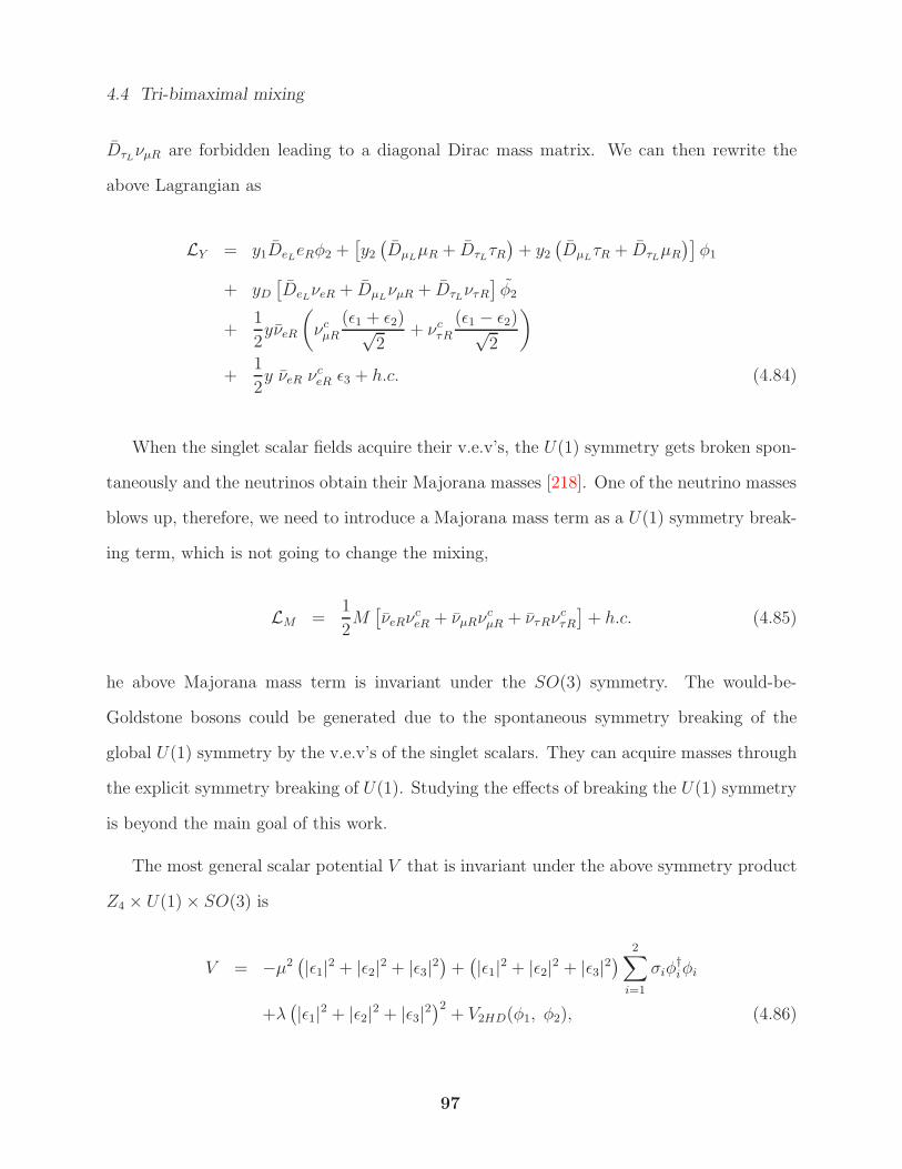
4.4 Tri-bimaximal mixing
DτLνµR are forbidden leading to a diagonal Dirac mass matrix. We can then rewrite the
above Lagrangian as
LY = y1DeLeRφ2 +[y2
(DµL
µR + DτLτR)+ y2
(DµL
τR + DτLµR
)]φ1
+ yD[DeLνeR + DµL
νµR + DτLντR]φ2
+1
2yνeR
(νcµR
(ǫ1 + ǫ2)√2
+ νcτR(ǫ1 − ǫ2)√
2
)
+1
2y νeR ν
ceR ǫ3 + h.c. (4.84)
When the singlet scalar fields acquire their v.e.v’s, the U(1) symmetry gets broken spon-
taneously and the neutrinos obtain their Majorana masses [218]. One of the neutrino masses
blows up, therefore, we need to introduce a Majorana mass term as a U(1) symmetry break-
ing term, which is not going to change the mixing,
LM =1
2M
[νeRν
ceR + νµRν
cµR + ντRν
cτR
]+ h.c. (4.85)
he above Majorana mass term is invariant under the SO(3) symmetry. The would-be-
Goldstone bosons could be generated due to the spontaneous symmetry breaking of the
global U(1) symmetry by the v.e.v’s of the singlet scalars. They can acquire masses through
the explicit symmetry breaking of U(1). Studying the effects of breaking the U(1) symmetry
is beyond the main goal of this work.
The most general scalar potential V that is invariant under the above symmetry product
Z4 × U(1)× SO(3) is
V = −µ2(|ǫ1|2 + |ǫ2|2 + |ǫ3|2
)+(|ǫ1|2 + |ǫ2|2 + |ǫ3|2
) 2∑
i=1
σiφ†iφi
+λ(|ǫ1|2 + |ǫ2|2 + |ǫ3|2
)2+ V2HD(φ1, φ2), (4.86)
97
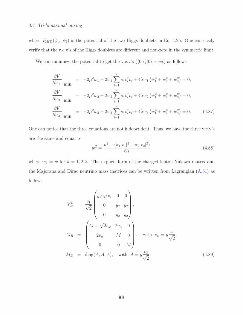
4.4 Tri-bimaximal mixing
where V2HD(φ1, φ2) is the potential of the two Higgs doublets in Eq. 4.25. One can easily
verify that the v.e.v’s of the Higgs doublets are different and non-zero in the symmetric limit.
We can minimize the potential to get the v.e.v’s (〈0|ǫ0k|0〉 = wk) as follows
∂V
∂|ǫ1|
∣∣∣∣min
= −2µ2w1 + 2w1
2∑
i=1
σiv†i vi + 4λw1
(w2
1 + w22 + w2
3
)= 0,
∂V
∂|ǫ2|
∣∣∣∣min
= −2µ2w2 + 2w2
2∑
i=1
σiv†i vi + 4λw2
(w2
1 + w22 + w2
3
)= 0,
∂V
∂|ǫ3|
∣∣∣∣min
= −2µ2w3 + 2w3
2∑
i=1
σiv†i vi + 4λw3
(w2
1 + w22 + w2
3
)= 0. (4.87)
One can notice that the three equations are not independent. Thus, we have the three v.e.v’s
are the same and equal to
w2 =µ2 − (σ1|v1|2 + σ2|v2|2)
6λ, (4.88)
where wk = w for k = 1, 2, 3. The explicit form of the charged lepton Yukawa matrix and
the Majorana and Dirac neutrino mass matrices can be written from Lagrangian (A.61) as
follows
Y L23 =
v1√2
y1v2/v1 0 0
0 y2 y2
0 y2 y2
,
MR =
M +√2vw 2vw 0
2vw M 0
0 0 M
, with vw = y
w√2,
MD = diag(A,A,A), with A = yv2√2. (4.89)
98
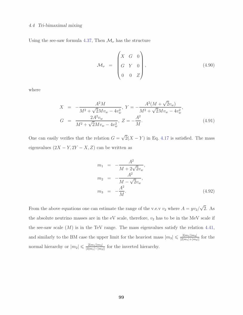
4.4 Tri-bimaximal mixing
Using the see-saw formula 4.37, Then Mν has the structure
Mν =
X G 0
G Y 0
0 0 Z
, (4.90)
where
X = − A2M
M2 +√2Mvw − 4v2w
, Y = − A2(M +√2vw)
M2 +√2Mvw − 4v2w
,
G =2A2vw
M2 +√2Mvw − 4v2w
, Z = −A2
M. (4.91)
One can easily verifies that the relation G =√2(X − Y ) in Eq. 4.17 is satisfied. The mass
eigenvalues (2X − Y, 2Y −X,Z) can be written as
m1 = − A2
M + 2√2vw
,
m2 = − A2
M −√2vw
,
m3 = −A2
M. (4.92)
From the above equations one can estimate the range of the v.e.v v2 where A = yv2/√2. As
the absolute neutrino masses are in the eV scale, therefore, v2 has to be in the MeV scale if
the see-saw scale (M) is in the TeV range. The mass eigenvalues satisfy the relation 4.41,
and similarly to the BM case the upper limit for the heaviest mass |m3| 6 3|m1||m2||2|m1|+|m2|| for the
normal hierarchy or |m2| 6 2|m1||m3||3|m1|−|m3|| for the inverted hierarchy.
99
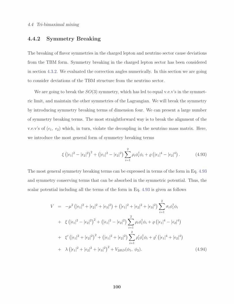
4.4 Tri-bimaximal mixing
4.4.2 Symmetry Breaking
The breaking of flavor symmetries in the charged lepton and neutrino sector cause deviations
from the TBM form. Symmetry breaking in the charged lepton sector has been considered
in section 4.3.2. We evaluated the correction angles numerically. In this section we are going
to consider deviations of the TBM structure from the neutrino sector.
We are going to break the SO(3) symmetry, which has led to equal v.e.v’s in the symmet-
ric limit, and maintain the other symmetries of the Lagrangian. We will break the symmetry
by introducing symmetry breaking terms of dimension four. We can present a large number
of symmetry breaking terms. The most straightforward way is to break the alignment of the
v.e.v’s of (ǫ1, ǫ2) which, in turn, violate the decoupling in the neutrino mass matrix. Here,
we introduce the most general form of symmetry breaking terms
ξ(|ǫ1|2 − |ǫ2|2
)2+(|ǫ1|2 − |ǫ2|2
) 2∑
i=1
ρiφ†iφi +
(|ǫ1|4 − |ǫ2|4
). (4.93)
The most general symmetry breaking terms can be expressed in terms of the form in Eq. 4.93
and symmetry conserving terms that can be absorbed in the symmetric potential. Thus, the
scalar potential including all the terms of the form in Eq. 4.93 is given as follows
V = −µ2(|ǫ1|2 + |ǫ2|2 + |ǫ3|2
)+(|ǫ1|2 + |ǫ2|2 + |ǫ3|2
) 2∑
i=1
σiφ†iφi
+ ξ(|ǫ1|2 − |ǫ2|2
)2+(|ǫ1|2 − |ǫ2|2
) 2∑
i=1
ρiφ†iφi +
(|ǫ1|4 − |ǫ2|4
)
+ ξ′(|ǫ1|2 + |ǫ2|2
)2+(|ǫ1|2 + |ǫ2|2
) 2∑
i=1
ρ′iφ†iφi + ′
(|ǫ1|4 + |ǫ2|4
)
+ λ(|ǫ1|2 + |ǫ2|2 + |ǫ3|2
)2+ V2HD(φ1, φ2). (4.94)
100
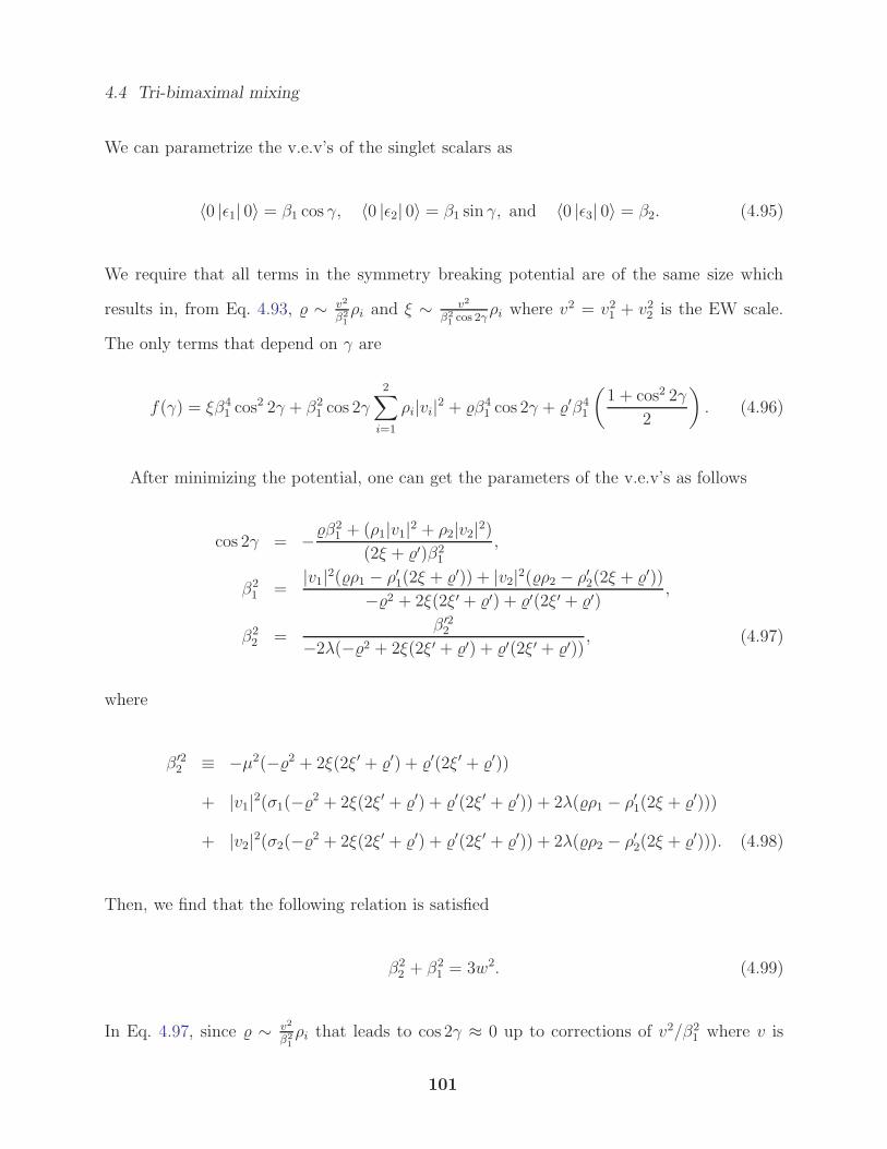
4.4 Tri-bimaximal mixing
We can parametrize the v.e.v’s of the singlet scalars as
〈0 |ǫ1| 0〉 = β1 cos γ, 〈0 |ǫ2| 0〉 = β1 sin γ, and 〈0 |ǫ3| 0〉 = β2. (4.95)
We require that all terms in the symmetry breaking potential are of the same size which
results in, from Eq. 4.93, ∼ v2
β21
ρi and ξ ∼ v2
β21 cos 2γ
ρi where v2 = v21 + v22 is the EW scale.
The only terms that depend on γ are
f(γ) = ξβ41 cos
2 2γ + β21 cos 2γ
2∑
i=1
ρi|vi|2 + β41 cos 2γ + ′β4
1
(1 + cos2 2γ
2
). (4.96)
After minimizing the potential, one can get the parameters of the v.e.v’s as follows
cos 2γ = −β21 + (ρ1|v1|2 + ρ2|v2|2)
(2ξ + ′)β21
,
β21 =
|v1|2(ρ1 − ρ′1(2ξ + ′)) + |v2|2(ρ2 − ρ′2(2ξ + ′))
−2 + 2ξ(2ξ′ + ′) + ′(2ξ′ + ′),
β22 =
β ′22
−2λ(−2 + 2ξ(2ξ′ + ′) + ′(2ξ′ + ′)), (4.97)
where
β ′22 ≡ −µ2(−2 + 2ξ(2ξ′ + ′) + ′(2ξ′ + ′))
+ |v1|2(σ1(−2 + 2ξ(2ξ′ + ′) + ′(2ξ′ + ′)) + 2λ(ρ1 − ρ′1(2ξ + ′)))
+ |v2|2(σ2(−2 + 2ξ(2ξ′ + ′) + ′(2ξ′ + ′)) + 2λ(ρ2 − ρ′2(2ξ + ′))). (4.98)
Then, we find that the following relation is satisfied
β22 + β2
1 = 3w2. (4.99)
In Eq. 4.97, since ∼ v2
β21
ρi that leads to cos 2γ ≈ 0 up to corrections of v2/β21 where v is
101
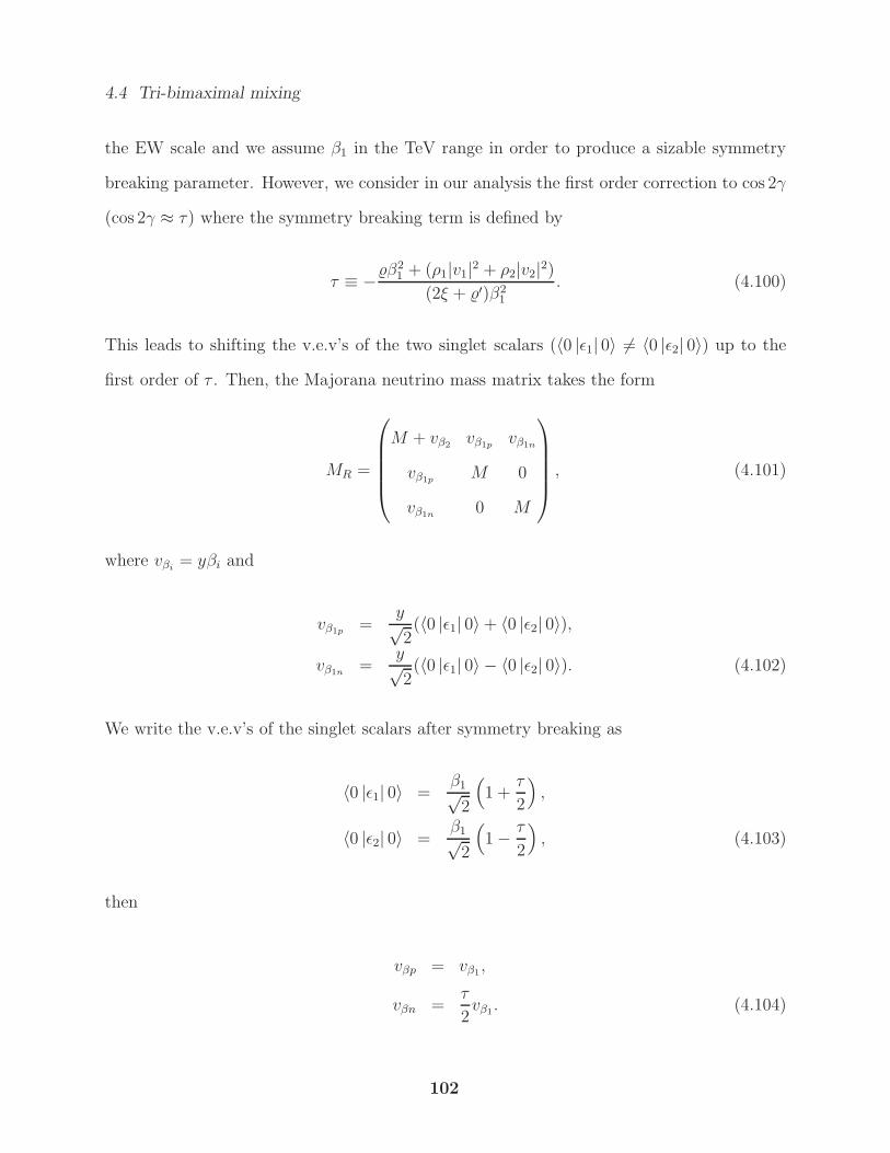
4.4 Tri-bimaximal mixing
the EW scale and we assume β1 in the TeV range in order to produce a sizable symmetry
breaking parameter. However, we consider in our analysis the first order correction to cos 2γ
(cos 2γ ≈ τ) where the symmetry breaking term is defined by
τ ≡ −β21 + (ρ1|v1|2 + ρ2|v2|2)
(2ξ + ′)β21
. (4.100)
This leads to shifting the v.e.v’s of the two singlet scalars (〈0 |ǫ1| 0〉 6= 〈0 |ǫ2| 0〉) up to the
first order of τ . Then, the Majorana neutrino mass matrix takes the form
MR =
M + vβ2vβ1p vβ1n
vβ1p M 0
vβ1n 0 M
, (4.101)
where vβi= yβi and
vβ1p =y√2(〈0 |ǫ1| 0〉+ 〈0 |ǫ2| 0〉),
vβ1n =y√2(〈0 |ǫ1| 0〉 − 〈0 |ǫ2| 0〉). (4.102)
We write the v.e.v’s of the singlet scalars after symmetry breaking as
〈0 |ǫ1| 0〉 =β1√2
(1 +
τ
2
),
〈0 |ǫ2| 0〉 =β1√2
(1− τ
2
), (4.103)
then
vβp = vβ1,
vβn =τ
2vβ1. (4.104)
102
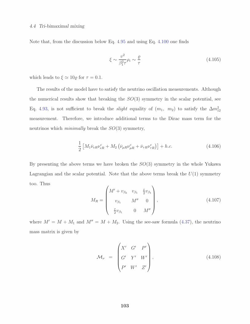
4.4 Tri-bimaximal mixing
Note that, from the discussion below Eq. 4.95 and using Eq. 4.100 one finds
ξ ∼ v2
β21τρi ∼
τ(4.105)
which leads to ξ ≃ 10 for τ = 0.1.
The results of the model have to satisfy the neutrino oscillation measurements. Although
the numerical results show that breaking the SO(3) symmetry in the scalar potential, see
Eq. 4.93, is not sufficient to break the slight equality of (m1, m2) to satisfy the ∆m212
measurement. Therefore, we introduce additional terms to the Dirac mass term for the
neutrinos which minimally break the SO(3) symmetry,
1
2
[M1νeRν
ceR +M2
(νµRν
cµR + ντRν
cτR
)]+ h.c. (4.106)
By presenting the above terms we have broken the SO(3) symmetry in the whole Yukawa
Lagrangian and the scalar potential. Note that the above terms break the U(1) symmetry
too. Thus
MR =
M ′ + vβ2vβ1
τ2vβ1
vβ1M ′′ 0
τ2vβ1
0 M ′′
, (4.107)
where M ′ = M +M1 and M ′′ = M +M2. Using the see-saw formula (4.37), the neutrino
mass matrix is given by
Mν =
X ′ G′ P ′
G′ Y ′ W ′
P ′ W ′ Z ′
, (4.108)
103
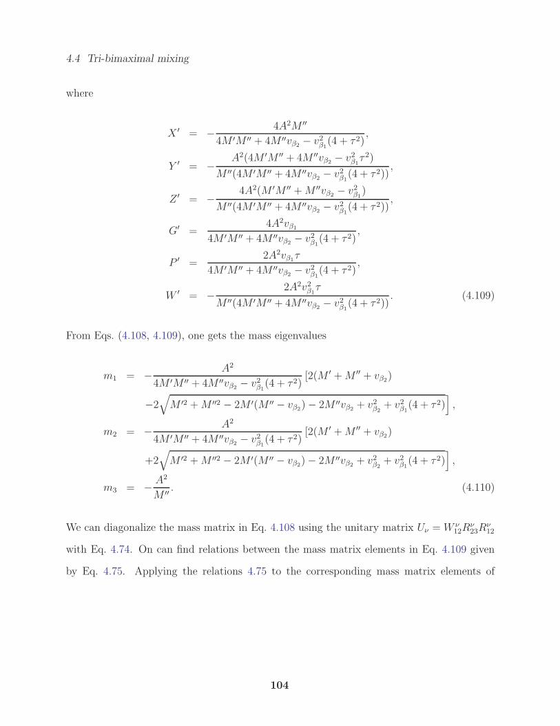
4.4 Tri-bimaximal mixing
where
X ′ = − 4A2M ′′
4M ′M ′′ + 4M ′′vβ2− v2β1
(4 + τ 2),
Y ′ = −A2(4M ′M ′′ + 4M ′′vβ2
− v2β1τ 2)
M ′′(4M ′M ′′ + 4M ′′vβ2− v2β1
(4 + τ 2)),
Z ′ = −4A2(M ′M ′′ +M ′′vβ2
− v2β1)
M ′′(4M ′M ′′ + 4M ′′vβ2− v2β1
(4 + τ 2)),
G′ =4A2vβ1
4M ′M ′′ + 4M ′′vβ2− v2β1
(4 + τ 2),
P ′ =2A2vβ1
τ
4M ′M ′′ + 4M ′′vβ2− v2β1
(4 + τ 2),
W ′ = −2A2v2β1
τ
M ′′(4M ′M ′′ + 4M ′′vβ2− v2β1
(4 + τ 2)). (4.109)
From Eqs. (4.108, 4.109), one gets the mass eigenvalues
m1 = − A2
4M ′M ′′ + 4M ′′vβ2− v2β1
(4 + τ 2)[2(M ′ +M ′′ + vβ2
)
−2√M ′2 +M ′′2 − 2M ′(M ′′ − vβ2
)− 2M ′′vβ2+ v2β2
+ v2β1(4 + τ 2)
],
m2 = − A2
4M ′M ′′ + 4M ′′vβ2− v2β1
(4 + τ 2)[2(M ′ +M ′′ + vβ2
)
+2√M ′2 +M ′′2 − 2M ′(M ′′ − vβ2
)− 2M ′′vβ2+ v2β2
+ v2β1(4 + τ 2)
],
m3 = − A2
M ′′ . (4.110)
We can diagonalize the mass matrix in Eq. 4.108 using the unitary matrix Uν =W ν12R
ν23R
ν12
with Eq. 4.74. On can find relations between the mass matrix elements in Eq. 4.109 given
by Eq. 4.75. Applying the relations 4.75 to the corresponding mass matrix elements of
104
4.4 Tri-bimaximal mixing
Mν = UνMdνU
†ν with Uν = W ν
12Rν23R
ν12 , one can get the two mixing angles
s23ν =
√3m1(m2 −m3)
m2(m1 −m3),
s12ν =
√−2m1m2 + 3m1m3 −m2m3
3m3(m1 −m2). (4.111)
Following Ref. [215], we expand the angles in Eq. 1.20 as
s13 =r√2, s12 =
1√3(1 + s), s23 =
1√2(1 + a), (4.112)
where the three real parameters r, s, a describe the deviations of the reactor, solar, and atmo-
spheric angles from their tri-bimaximal values. We use global fits of the mixing parameters
with 3σ significance [47]
0.18 < r < 0.26, −0.10 < s < 0.05, −0.15 < a < 0.17. (4.113)
To first order in r, s, a the lepton mixing matrix can be written as [215],
U ≈
√23(1− 1
2s) 1√
3(1 + s) 1√
2re−iδ
− 1√6(1 + s− a+ reiδ) 1√
3(1− 1
2s− a− 1
2reiδ) 1√
2(1 + a)
1√6(1 + s+ a− reiδ) − 1√
3(1− 1
2s+ a+ 1
2reiδ) 1√
2(1− a)
. (4.114)
We are not going to consider CP violation in this work, thus, we assume that δ = 0. We can
write the parameters (r, s, a) in terms of the elements of the mixing matrix,
r = −1− s+ a−√6U21,
s = −1 +√3U12,
a = −1 +√2U23. (4.115)
105
4.4 Tri-bimaximal mixing
Now, we can calculate the full deviation of the leptonic mixing coming from the charged
lepton and neutrino sector. We obtain the elements of the lepton mixing matrix
UPMNS = U †l Uν , (4.116)
with Uℓ = W l23R
l23R
l13R
l12 and Uν =W ν
12Rν23R
ν12. Thus, up to the first order one can get
r ≈ −s12l +√
2
3s23ν + s13l,
s ≈ −s12l +√2s12ν − s13l,
a ≈ −s23l +√
2
3s23ν . (4.117)
In section 4.3.2, it was found that the contribution of the charged lepton sector, with
δ = 0, is give as
• For z = 1.8: s12l ≈ ±0.44, s13l ≈ ∓0.0012, s23l ≈ −0.053,
• For z = 1.7: s12l ≈ ±0.48, s13l ≈ ∓0.0013, s23l ≈ −0.050,
where z is an arbitrary parameter with a value around 2. We can check the contributions of
the charged leptons, Uℓ = W l23R
l23R
l13R
l12, without corrections from the neutrino sector, i.e.
Uν = W ν12. By substituting the above values in Eq. 4.117 up to the first order one gets
• For z = 1.8: r ≈ 0.44, s ≈ 0.44, a ≈ 0.053,
• For z = 1.7: r ≈ 0.48, s ≈ 0.48, a ≈ 0.050,
The results above do not match the experimental values where the charged lepton sector
introduces a large correction to the mixing angles θ13 and θ12. Thus, it becomes necessary
to combine the contributions come from the charged lepton and neutrino sector in order to
calculate the full deviation from the TBM mixing.
106
4.5 Conclusion
4.4.3 Numerical results
In the case of degenerate neutrino masses m1 ≈ m2 ≈ m3, one can find from Eq. 4.18 that
a ≈ b ≈ c. This leads to a diagonalized neutrino mass matrix Mν ≈ diag (a, a, a). That
means the lepton mixing matrix does not include a contribution from the neutrino sector,
which is inconsistent with the experimental data. Thus, in the symmetric limit our model
excludes the case of the degenerate neutrino masses.
The numerics goes following the method used in the BM case. The results support the
normal mass hierarchy. The figures show that the scale of the neutrino masses is in the
few meV to ∼ 50 meV range (meV= 10−3eV). Also, the full contribution from both the
charged lepton and neutrino sector accommodates the measurements of the mixing angles.
The graphs (4.4, 4.5) show that the see-saw scales (M ′, M ′′) are in the TeV range, and
the extra Higgs that generates the Dirac neutrino masses has v.e.v (v2), included in A, in
the MeV scale 3. Also, they indicate that the v.e.v’s of the singlet scalar fields (vβ1, vβ2)
are in the TeV scale 4. We plot Mβ versus Σmi and Mee versus mlight, where mlight is the
lightest neutrino mass which is m1 in this model. The graphs show that Σmi ≈ 60 meV and
Mee < Mβ and Mee < 0.40 eV [216].
4.5 Conclusion
In this work we presented a model for leptonic mixing which accommodates the sizable
neutrino mixing angle θ13 recently measured. We worked in a basis where the charged lepton
mass matrix is not diagonal and proposed an explicit structure for the charged lepton mass
matrix which is 2-3 symmetric except for a single breaking of this symmetry by the muon
mass. We identified a flavor symmetric limit for the mass matrices where the first generation
3Higgs doublet with a small v.e.v has been discussed in the literatures [219].4Several papers have introduced neutrino mixing models in the TeV scale (for review see Refs. [220]).
107
4.5 Conclusion
is decoupled from the other two in the charged lepton sector while in the neutrino sector
the third generation is decoupled from the first two generations. The leptonic mixing in the
symmetric limit was shown to have, among other structures, the bi-maximal (BM) and the
tri-bimaximal (TBM) mixing.
In the BM case, a model that extended the SM by three right handed neutrinos, an extra
Higgs doublet, and two singlet scalars was introduced to generate the leptonic mixing. In the
symmetric limit the model had two Z2 symmetries in addition to the µ−τ symmetry and the
BM leptonic mixing was obtained when the two singlet scalars got equal v.e.v’s. Symmetry
breaking effects were included in the charged lepton sector via higher dimensional operators
that generated a µ− τ symmetric mass matrix except for a single breaking due to the finite
muon mass. In the neutrino sector, symmetry breaking was included via slightly different
v.e.v’s for the two singlet scalars. To explain the ∆m2 data, two different Majorana mass
terms, one for νe and one for νµ and ντ , was used keeping in mind that the µ− τ symmetry
fixes the Majorana mass terms for the νµ and ντ to be the same.
In the TBM case, we fixed the neutrino mass matrix to have a decoupling of the first
two generations from the third one, and under a certain condition we generated the lepton
mixing in the symmetric limit with the TBM structure. This model was described by the
Lagrangian that extended the SM by three right-handed neutrinos, an extra Higgs doublet,
and three complex singlet scalar fields. Also, the symmetry group of the SM was extended
by the product of the symmetries Z4 ×U(1). The symmetry breaking in the charged lepton
sector did not fix the data by introducing a large contribution to the mixing angles θ13 and
θ12. Thereafter, by breaking the SO(3) symmetry in the effective potential and violating the
alignment of the v.e.v’s of the singlet scalars, the contribution of the neutrino sector was
introduced to accommodate the measurements.
A fit to the experimental measurements showed in both the cases that our model predicted
normal hierarchy for the neutrino masses with the masses being in the few meV to ∼ 50
108

4.5 Conclusion
meV range. The Majorana mass terms as well as the v.e.v’s of the singlet scalar fields were
predicted to be in the TeV scale and consequently the v.e.v of the second Higgs doublet was
shown to be in the MeV range. We calculated predictions for the mass-dependent observables
(Σmi), (Mβ) and (Mee). We found that Σmi ≈ 0.06 eV, Mee < Mβ , and Mee < 0.40 eV.
109
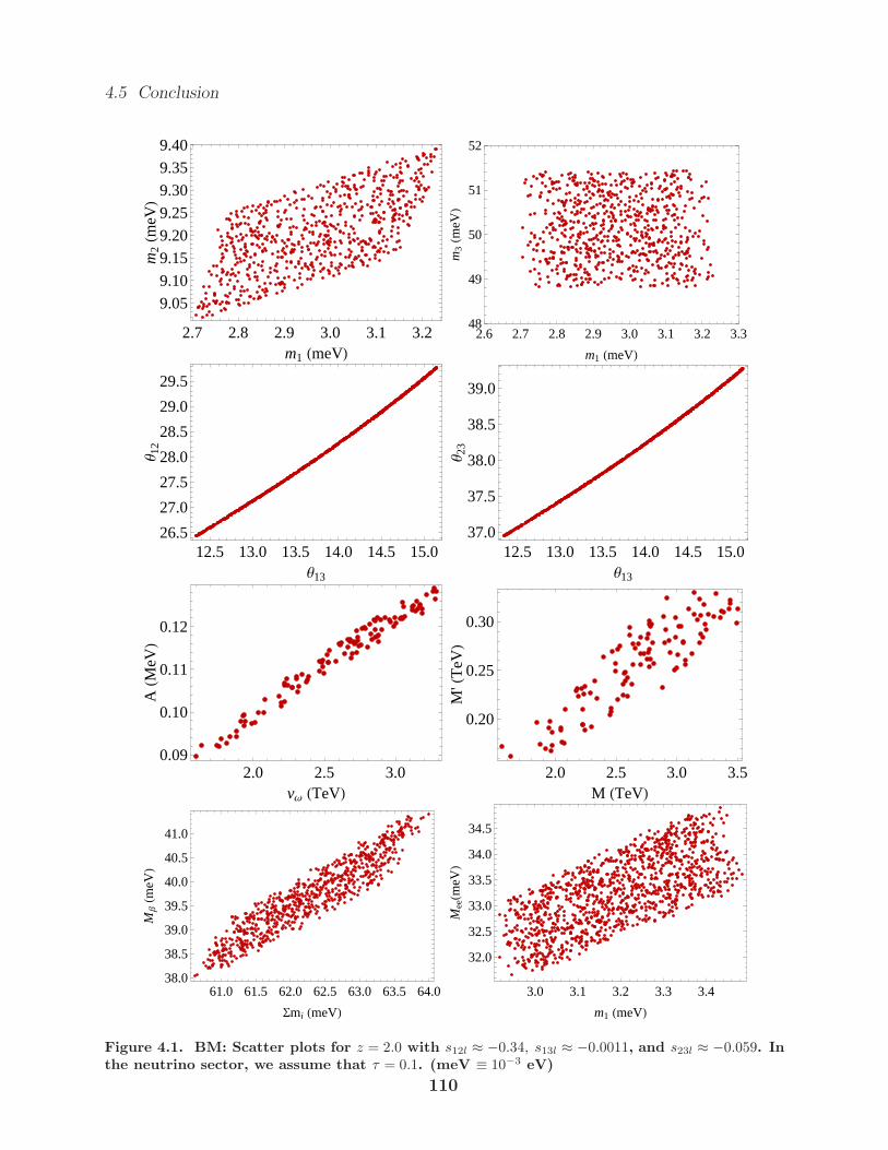
4.5 Conclusion
2.7 2.8 2.9 3.0 3.1 3.2
9.05
9.10
9.15
9.20
9.25
9.30
9.35
9.40
m1 HmeVL
m2Hm
eVL
2.6 2.7 2.8 2.9 3.0 3.1 3.2 3.348
49
50
51
52
m1 HmeVL
m3Hm
eVL
12.5 13.0 13.5 14.0 14.5 15.026.5
27.0
27.5
28.0
28.5
29.0
29.5
Θ13
Θ 12
12.5 13.0 13.5 14.0 14.5 15.037.0
37.5
38.0
38.5
39.0
Θ13
Θ 23
2.0 2.5 3.00.09
0.10
0.11
0.12
vΩ HTeVL
AHM
eVL
2.0 2.5 3.0 3.5
0.20
0.25
0.30
M HTeVL
M'H
TeVL
61.0 61.5 62.0 62.5 63.0 63.5 64.038.0
38.5
39.0
39.5
40.0
40.5
41.0
Smi HmeVL
MΒHm
eVL
3.0 3.1 3.2 3.3 3.4
32.0
32.5
33.0
33.5
34.0
34.5
m1 HmeVL
MeeHm
eVL
Figure 4.1. BM: Scatter plots for z = 2.0 with s12l ≈ −0.34, s13l ≈ −0.0011, and s23l ≈ −0.059. Inthe neutrino sector, we assume that τ = 0.1. (meV ≡ 10−3 eV)
110
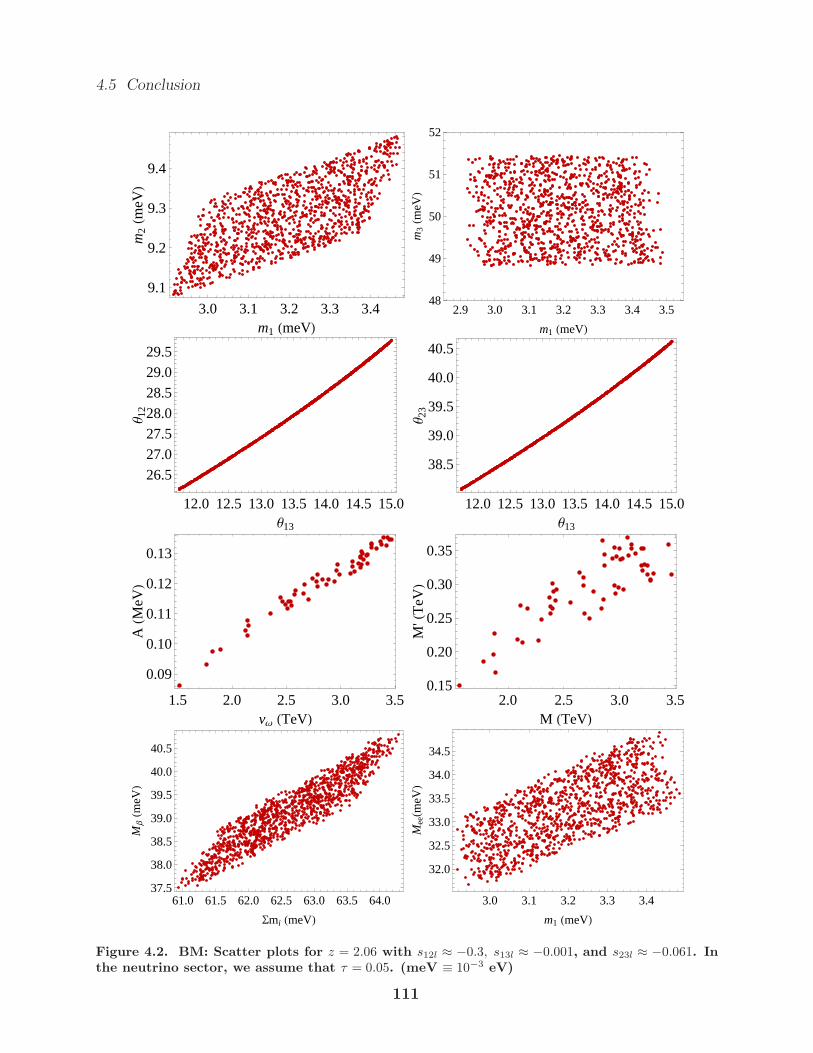
4.5 Conclusion
3.0 3.1 3.2 3.3 3.4
9.1
9.2
9.3
9.4
m1 HmeVL
m2Hm
eVL
2.9 3.0 3.1 3.2 3.3 3.4 3.548
49
50
51
52
m1 HmeVL
m3Hm
eVL
12.0 12.5 13.0 13.5 14.0 14.5 15.0
26.5
27.0
27.5
28.0
28.5
29.0
29.5
Θ13
Θ 12
12.0 12.5 13.0 13.5 14.0 14.5 15.0
38.5
39.0
39.5
40.0
40.5
Θ13
Θ 23
1.5 2.0 2.5 3.0 3.5
0.09
0.10
0.11
0.12
0.13
vΩ HTeVL
AHM
eVL
2.0 2.5 3.0 3.50.15
0.20
0.25
0.30
0.35
M HTeVL
M'H
TeVL
61.0 61.5 62.0 62.5 63.0 63.5 64.037.5
38.0
38.5
39.0
39.5
40.0
40.5
Smi HmeVL
MΒHm
eVL
3.0 3.1 3.2 3.3 3.4
32.0
32.5
33.0
33.5
34.0
34.5
m1 HmeVL
MeeHm
eVL
Figure 4.2. BM: Scatter plots for z = 2.06 with s12l ≈ −0.3, s13l ≈ −0.001, and s23l ≈ −0.061. Inthe neutrino sector, we assume that τ = 0.05. (meV ≡ 10−3 eV)
111
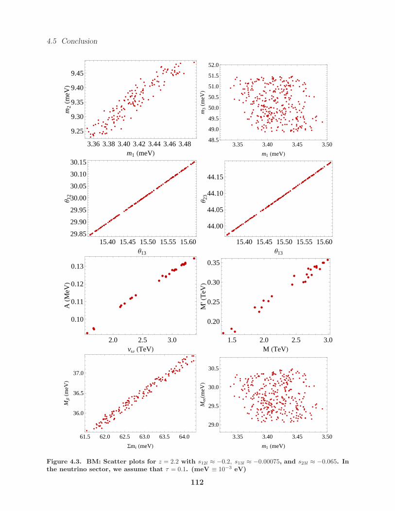
4.5 Conclusion
3.36 3.38 3.40 3.42 3.44 3.46 3.48
9.25
9.30
9.35
9.40
9.45
m1 HmeVL
m2Hm
eVL
3.35 3.40 3.45 3.5048.5
49.0
49.5
50.0
50.5
51.0
51.5
52.0
m1 HmeVL
m3Hm
eVL
15.40 15.45 15.50 15.55 15.6029.85
29.90
29.95
30.00
30.05
30.10
30.15
Θ13
Θ 12
15.40 15.45 15.50 15.55 15.60
44.00
44.05
44.10
44.15
Θ13
Θ 23
2.0 2.5 3.0
0.10
0.11
0.12
0.13
vΩ HTeVL
AHM
eVL
1.5 2.0 2.5 3.0
0.20
0.25
0.30
0.35
M HTeVL
M'H
TeVL
61.5 62.0 62.5 63.0 63.5 64.0
36.0
36.5
37.0
Smi HmeVL
MΒHm
eVL
3.35 3.40 3.45 3.50
29.0
29.5
30.0
30.5
m1 HmeVL
MeeHm
eVL
Figure 4.3. BM: Scatter plots for z = 2.2 with s12l ≈ −0.2, s13l ≈ −0.00075, and s23l ≈ −0.065. Inthe neutrino sector, we assume that τ = 0.1. (meV ≡ 10−3 eV)
112
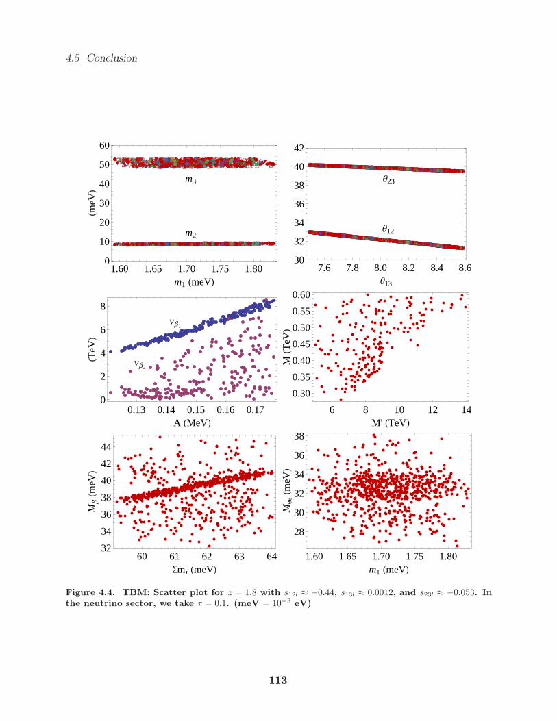
4.5 Conclusion
ò
ò
ô
ô
á
á
í
í
æ
æ
í
í
í
í
ç
ç
õ
õ
à
à
à
à
ó
ó
õ
õ
ì
ì
æ
æ
á
á
í
í
õ
õ
ì
ì
æ
æ
æ
æ
æ
æ
ò
ò
à
à
æ
æ
ì
ì
ò
ò
á
á
ô
ô
á
á
ì
ì
ì
ì
í
í
ç
ç
ò
ò
ò
ò
à
à
ò
ò
ò
ò
æ
æ
ó
ó
í
í
ó
ó
ó
ó
õ
õ
ì
ì
ô
ô
ó
ó
ô
ô
õ
õ
õ
õ
æ
æ
ó
ó
ç
ç
ô
ô
à
à
à
à
í
í
æ
æ
ó
ó
í
í
ç
ç
ò
ò
ç
ç
æ
æ
ó
ó
à
à
ç
ç
á
á
í
í
õ
õ
à
à
ò
ò
ô
ô
à
à
á
á
ì
ì
ò
ò
õ
õ
æ
æ
í
í
ì
ì
ç
ç
æ
æ
ò
ò
à
à
à
à
ó
ó
à
à
á
á
ó
ó
õ
õ
ì
ì
ó
ó
ô
ô
ç
ç
ì
ì
æ
æ
æ
æ
ì
ì
á
á
æ
æ
ç
ç
ó
ó
í
í
æ
æ
õ
õ
æ
æ
á
á
ì
ì
à
à
ó
ó
á
á
ç
ç
ç
ç
õ
õ
ô
ô
ç
ç
á
á
ô
ô
ç
ç
õ
õ
ì
ì
õ
õ
ì
ì
ó
ó
æ
æ
ç
ç
ò
ò
ô
ô
ô
ô
ô
ô
ì
ì
ò
ò
æ
æ
í
í
ì
ì
í
í
ó
ó
ç
ç
õ
õ
æ
æ
à
à
õ
õ
ç
ç
ç
ç
õ
õ
ç
ç
ô
ô
õ
õ
õ
õ
ò
ò
ò
ò
ô
ô
ò
ò
à
à
ì
ì
á
á
õ
õ
ì
ì
ó
ó
ô
ô
í
í
à
à
ì
ì
ó
ó
ô
ô
í
í
á
á
à
à
í
í
ì
ì
õ
õ
õ
õ
ó
ó
ò
ò
í
í
æ
æ
á
á
æ
æ
æ
æ
ô
ô
ò
ò
ò
ò
ì
ì
õ
õ
ò
ò
í
í
ì
ì
à
à
í
í
ì
ì
æ
æ
ì
ì
á
á
ô
ô
à
à
æ
æ
ç
ç
æ
æ
ò
ò
ô
ô
õ
õ
æ
æ
à
à
í
í
ô
ô
á
á
à
à
ç
ç
ó
ó
ç
ç
á
á
ô
ô
ó
ó
õ
õ
ç
ç
í
í
à
à
ì
ì
ç
ç
à
à
ç
ç
ô
ô
á
á
ç
ç
ì
ì
ò
ò
í
í
ç
ç
ò
ò
á
á
à
à
õ
õ
ì
ì
æ
æ
ó
ó
ó
ó
ò
ò
á
á
ô
ô
æ
æ
ô
ô
æ
æ
ò
ò
ó
ó
ô
ô
ô
ô
ó
ó
ò
ò
ò
ò
à
à
ó
ó
ó
ó
ì
ì
ó
ó
á
á
õ
õ
æ
æ
ô
ô
ò
ò
í
í
æ
æ
í
í
à
à
æ
æ
ì
ì
ç
ç
ì
ì
á
á
ô
ô
ô
ô
í
í
ó
ó
ô
ô
ò
ò
õ
õ
æ
æ
ô
ô
à
à
à
à
õ
õ
á
á
ì
ì
õ
õ
ô
ô
á
á
í
í
õ
õ
ì
ì
ì
ì
à
à
à
à
í
í
õ
õ
ì
ì
ò
ò
æ
æ
õ
õ
ç
ç
à
à
ó
ó
æ
æ
à
à
ì
ì
ì
ì
à
à
á
á
á
á
ì
ì
ô
ô
æ
æ
õ
õ
à
à
á
á
à
à
ò
ò
õ
õ
á
á
ò
ò
í
í
ô
ô
ó
ó
ì
ì
ç
ç
ç
ç
õ
õ
ô
ô
á
á
æ
æ
à
à
ò
ò
ô
ô
ì
ì
ò
ò
ì
ì
ç
ç
õ
õ
ì
ì
ò
ò
ô
ô
õ
õ
æ
æ
à
à
á
á
õ
õ
í
í
ò
ò
á
á
à
à
í
í
ô
ô
ç
ç
ç
ç
à
à
í
í
à
à
á
á
ó
ó
ó
ó
æ
æ
ô
ô
ó
ó
ì
ì
ô
ô
æ
æ
æ
æ
ô
ô
õ
õ
ó
ó
ó
ó
ç
ç
á
á
í
í
á
á
à
à
ç
ç
à
à
õ
õ
ç
ç
ì
ì
ó
ó
à
à
à
à
ó
ó
ó
ó
á
á
í
í
ç
ç
í
í
ç
ç
æ
æ
æ
æ
ì
ì
ó
ó
õ
õ
æ
æ
ì
ì
æ
æ
ó
ó
æ
æ
í
í
ì
ì
í
í
ó
ó
æ
æ
à
à
ç
ç
ì
ì
ç
ç
ò
ò
ì
ì
õ
õ
ì
ì
ó
ó
ó
ó
á
á
ç
ç
ó
ó
õ
õ
í
í
æ
æ
á
á
à
à
ì
ì
ó
ó
õ
õ
ó
ó
æ
æ
õ
õ
ò
ò
ò
ò
á
á
í
í
í
í
á
á
õ
õ
æ
æ
ì
ì
ò
ò
à
à
æ
æ
õ
õ
æ
æ
ô
ô
í
í
ò
ò
ç
ç
ó
ó
í
í
à
à
í
í
ì
ì
ô
ô
ô
ô
ì
ì
ò
ò
í
í
æ
æ
ç
ç
ç
ç
ò
ò
í
í
ó
ó
ô
ô
ô
ô
ó
ó
ó
ó
à
à
í
í
ò
ò
á
á
æ
æ
à
à
õ
õ
õ
õ
ó
ó
ô
ô
ó
ó
í
í
õ
õ
ó
ó
ô
ô
à
à
à
à
ò
ò
æ
æ
à
à
ç
ç
ì
ì
ò
ò
æ
æ
í
í
á
á
ó
ó
æ
æ
ç
ç
ç
ç
á
á
ô
ô
í
í
ô
ô
ç
ç
ó
ó
æ
æ
ò
ò
ì
ì
á
á
í
í
à
à
ô
ô
í
í
æ
æ
ò
ò
ô
ô
ç
ç
í
í
æ
æ
ç
ç
í
í
ç
ç
æ
æ
ç
ç
í
í
í
í
ç
ç
á
á
æ
æ
æ
æ
á
á
ó
ó
ó
ó
á
á
õ
õ
à
à
à
à
ò
ò
ç
ç
ò
ò
á
á
á
á
ô
ô
ô
ô
æ
æ
á
á
à
à
à
à
ç
ç
æ
æ
ç
ç
à
à
á
á
æ
æ
æ
æ
ç
ç
á
á
à
à
í
í
ó
ó
ó
ó
ì
ì
ì
ì
æ
æ
æ
æ
ó
ó
ô
ô
à
à
æ
æ
õ
õ
ó
ó
à
à
í
í
ç
ç
ò
ò
æ
æ
í
í
ó
ó
ì
ì
æ
æ
í
í
ô
ô
í
í
ì
ì
í
í
à
à
ò
ò
ì
ì
æ
æ
æ
æ
à
à
ç
ç
õ
õ
æ
æ
ô
ô
í
í
ç
ç
í
í
à
à
æ
æ
æ
æ
ó
ó
ò
ò
ô
ô
ó
ó
ì
ì
õ
õ
ì
ì
ò
ò
ò
ò
á
á
ó
ó
ì
ì
ó
ó
ó
ó
ò
ò
õ
õ
à
à
á
á
á
á
ç
ç
ç
ç
á
á
ô
ô
æ
æ
á
á
á
á
à
à
õ
õ
ò
ò
á
á
ç
ç
í
í
ì
ì
ì
ì
æ
æ
ò
ò
á
á
í
í
ì
ì
ò
ò
ô
ô
ò
ò
õ
õ
ç
ç
í
í
ì
ì
ò
ò
á
á
ò
ò
ó
ó
ç
ç
ì
ì
ç
ç
æ
æ
ò
ò
ô
ô
à
à
ì
ì
á
á
í
í
õ
õ
ó
ó
à
à
ó
ó
æ
æ
ç
ç
õ
õ
à
à
ò
ò
ò
ò
ó
ó
ô
ô
õ
õ
à
à
ó
ó
ì
ì
ó
ó
ó
ó
ô
ô
ì
ì
ó
ó
æ
æ
ç
ç
í
í
í
í
á
á
í
í
ç
ç
à
à
õ
õ
õ
õ
ô
ô
á
á
ç
ç
ò
ò
ó
ó
à
à
ì
ì
à
à
á
á
æ
æ
ò
ò
à
à
õ
õ
í
í
á
á
à
à
õ
õ
á
á
ò
ò
ì
ì
ò
ò
æ
æ
ò
ò
ó
ó
æ
æ
ó
ó
í
í
í
í
í
í
æ
æ
æ
æ
ó
ó
ç
ç
ç
ç
ó
ó
ì
ì
í
í
á
á
ô
ô
ì
ì
ó
ó
í
í
ç
ç
ì
ì
ô
ô
ô
ô
í
í
ç
ç
õ
õ
á
á
ó
ó
à
à
à
à
á
á
õ
õ
m3
m2
1.60 1.65 1.70 1.75 1.800
10
20
30
40
50
60
m1 HmeVL
HmeVL
ò
ò
ô
ô
á
á
í
í
æ
æ
í
í
í
í
ç
ç
õ
õ
à
à
à
à
ó
ó
õ
õ
ì
ì
æ
æ
á
á
í
í
õ
õ
ì
ì
æ
æ
æ
æ
æ
æ
ò
ò
à
à
æ
æ
ì
ì
ò
ò
á
á
ô
ô
á
á
ì
ì
ì
ì
í
í
ç
ç
ò
ò
ò
ò
à
à
ò
ò
ò
ò
æ
æ
ó
ó
í
í
ó
ó
ó
ó
õ
õ
ì
ì
ô
ô
ó
ó
ô
ô
õ
õ
õ
õ
æ
æ
ó
ó
ç
ç
ô
ô
à
à
à
à
í
í
æ
æ
ó
ó
í
í
ç
ç
ò
ò
ç
ç
æ
æ
ó
ó
à
à
ç
ç
á
á
í
í
õ
õ
à
à
ò
ò
ô
ô
à
à
á
á
ì
ì
ò
ò
õ
õ
æ
æ
í
í
ì
ì
ç
ç
æ
æ
ò
ò
à
à
à
à
ó
ó
à
à
á
á
ó
ó
õ
õ
ì
ì
ó
ó
ô
ô
ç
ç
ì
ì
æ
æ
æ
æ
ì
ì
á
á
æ
æ
ç
ç
ó
ó
í
í
æ
æ
õ
õ
æ
æ
á
á
ì
ì
à
à
ó
ó
á
á
ç
ç
ç
ç
õ
õ
ô
ô
ç
ç
á
á
ô
ô
ç
ç
õ
õ
ì
ì
õ
õ
ì
ì
ó
ó
æ
æ
ç
ç
ò
ò
ô
ô
ô
ô
ô
ô
ì
ì
ò
ò
æ
æ
í
í
ì
ì
í
í
ó
ó
ç
ç
õ
õ
æ
æ
à
à
õ
õ
ç
ç
ç
ç
õ
õ
ç
ç
ô
ô
õ
õ
õ
õ
ò
ò
ò
ò
ô
ô
ò
ò
à
à
ì
ì
á
á
õ
õ
ì
ì
ó
ó
ô
ô
í
í
à
à
ì
ì
ó
ó
ô
ô
í
í
á
á
à
à
í
í
ì
ì
õ
õ
õ
õ
ó
ó
ò
ò
í
í
æ
æ
á
á
æ
æ
æ
æ
ô
ô
ò
ò
ò
ò
ì
ì
õ
õ
ò
ò
í
í
ì
ì
à
à
í
í
ì
ì
æ
æ
ì
ì
á
á
ô
ô
à
à
æ
æ
ç
ç
æ
æ
ò
ò
ô
ô
õ
õ
æ
æ
à
à
í
í
ô
ô
á
á
à
à
ç
ç
ó
ó
ç
ç
á
á
ô
ô
ó
ó
õ
õ
ç
ç
í
í
à
à
ì
ì
ç
ç
à
à
ç
ç
ô
ô
á
á
ç
ç
ì
ì
ò
ò
í
í
ç
ç
ò
ò
á
á
à
à
õ
õ
ì
ì
æ
æ
ó
ó
ó
ó
ò
ò
á
á
ô
ô
æ
æ
ô
ô
æ
æ
ò
ò
ó
ó
ô
ô
ô
ô
ó
ó
ò
ò
ò
ò
à
à
ó
ó
ó
ó
ì
ì
ó
ó
á
á
õ
õ
æ
æ
ô
ô
ò
ò
í
í
æ
æ
í
í
à
à
æ
æ
ì
ì
ç
ç
ì
ì
á
á
ô
ô
ô
ô
í
í
ó
ó
ô
ô
ò
ò
õ
õ
æ
æ
ô
ô
à
à
à
à
õ
õ
á
á
ì
ì
õ
õ
ô
ô
á
á
í
í
õ
õ
ì
ì
ì
ì
à
à
à
à
í
í
õ
õ
ì
ì
ò
ò
æ
æ
õ
õ
ç
ç
à
à
ó
ó
æ
æ
à
à
ì
ì
ì
ì
à
à
á
á
á
á
ì
ì
ô
ô
æ
æ
õ
õ
à
à
á
á
à
à
ò
ò
õ
õ
á
á
ò
ò
í
í
ô
ô
ó
ó
ì
ì
ç
ç
ç
ç
õ
õ
ô
ô
á
á
æ
æ
à
à
ò
ò
ô
ô
ì
ì
ò
ò
ì
ì
ç
ç
õ
õ
ì
ì
ò
ò
ô
ô
õ
õ
æ
æ
à
à
á
á
õ
õ
í
í
ò
ò
á
á
à
à
í
í
ô
ô
ç
ç
ç
ç
à
à
í
í
à
à
á
á
ó
ó
ó
ó
æ
æ
ô
ô
ó
ó
ì
ì
ô
ô
æ
æ
æ
æ
ô
ô
õ
õ
ó
ó
ó
ó
ç
ç
á
á
í
í
á
á
à
à
ç
ç
à
à
õ
õ
ç
ç
ì
ì
ó
ó
à
à
à
à
ó
ó
ó
ó
á
á
í
í
ç
ç
í
í
ç
ç
æ
æ
æ
æ
ì
ì
ó
ó
õ
õ
æ
æ
ì
ì
æ
æ
ó
ó
æ
æ
í
í
ì
ì
í
í
ó
ó
æ
æ
à
à
ç
ç
ì
ì
ç
ç
ò
ò
ì
ì
õ
õ
ì
ì
ó
ó
ó
ó
á
á
ç
ç
ó
ó
õ
õ
í
í
æ
æ
á
á
à
à
ì
ì
ó
ó
õ
õ
ó
ó
æ
æ
õ
õ
ò
ò
ò
ò
á
á
í
í
í
í
á
á
õ
õ
æ
æ
ì
ì
ò
ò
à
à
æ
æ
õ
õ
æ
æ
ô
ô
í
í
ò
ò
ç
ç
ó
ó
í
í
à
à
í
í
ì
ì
ô
ô
ô
ô
ì
ì
ò
ò
í
í
æ
æ
ç
ç
ç
ç
ò
ò
í
í
ó
ó
ô
ô
ô
ô
ó
ó
ó
ó
à
à
í
í
ò
ò
á
á
æ
æ
à
à
õ
õ
õ
õ
ó
ó
ô
ô
ó
ó
í
í
õ
õ
ó
ó
ô
ô
à
à
à
à
ò
ò
æ
æ
à
à
ç
ç
ì
ì
ò
ò
æ
æ
í
í
á
á
ó
ó
æ
æ
ç
ç
ç
ç
á
á
ô
ô
í
í
ô
ô
ç
ç
ó
ó
æ
æ
ò
ò
ì
ì
á
á
í
í
à
à
ô
ô
í
í
æ
æ
ò
ò
ô
ô
ç
ç
í
í
æ
æ
ç
ç
í
í
ç
ç
æ
æ
ç
ç
í
í
í
í
ç
ç
á
á
æ
æ
æ
æ
á
á
ó
ó
ó
ó
á
á
õ
õ
à
à
à
à
ò
ò
ç
ç
ò
ò
á
á
á
á
ô
ô
ô
ô
æ
æ
á
á
à
à
à
à
ç
ç
æ
æ
ç
ç
à
à
á
á
æ
æ
æ
æ
ç
ç
á
á
à
à
í
í
ó
ó
ó
ó
ì
ì
ì
ì
æ
æ
æ
æ
ó
ó
ô
ô
à
à
æ
æ
õ
õ
ó
ó
à
à
í
í
ç
ç
ò
ò
æ
æ
í
í
ó
ó
ì
ì
æ
æ
í
í
ô
ô
í
í
ì
ì
í
í
à
à
ò
ò
ì
ì
æ
æ
æ
æ
à
à
ç
ç
õ
õ
æ
æ
ô
ô
í
í
ç
ç
í
í
à
à
æ
æ
æ
æ
ó
ó
ò
ò
ô
ô
ó
ó
ì
ì
õ
õ
ì
ì
ò
ò
ò
ò
á
á
ó
ó
ì
ì
ó
ó
ó
ó
ò
ò
õ
õ
à
à
á
á
á
á
ç
ç
ç
ç
á
á
ô
ô
æ
æ
á
á
á
á
à
à
õ
õ
ò
ò
á
á
ç
ç
í
í
ì
ì
ì
ì
æ
æ
ò
ò
á
á
í
í
ì
ì
ò
ò
ô
ô
ò
ò
õ
õ
ç
ç
í
í
ì
ì
ò
ò
á
á
ò
ò
ó
ó
ç
ç
ì
ì
ç
ç
æ
æ
ò
ò
ô
ô
à
à
ì
ì
á
á
í
í
õ
õ
ó
ó
à
à
ó
ó
æ
æ
ç
ç
õ
õ
à
à
ò
ò
ò
ò
ó
ó
ô
ô
õ
õ
à
à
ó
ó
ì
ì
ó
ó
ó
ó
ô
ô
ì
ì
ó
ó
æ
æ
ç
ç
í
í
í
í
á
á
í
í
ç
ç
à
à
õ
õ
õ
õ
ô
ô
á
á
ç
ç
ò
ò
ó
ó
à
à
ì
ì
à
à
á
á
æ
æ
ò
ò
à
à
õ
õ
í
í
á
á
à
à
õ
õ
á
á
ò
ò
ì
ì
ò
ò
æ
æ
ò
ò
ó
ó
æ
æ
ó
ó
í
í
í
í
í
í
æ
æ
æ
æ
ó
ó
ç
ç
ç
ç
ó
ó
ì
ì
í
í
á
á
ô
ô
ì
ì
ó
ó
í
í
ç
ç
ì
ì
ô
ô
ô
ô
í
í
ç
ç
õ
õ
á
á
ó
ó
à
à
à
à
á
á
õ
õ
Θ12
Θ23
7.6 7.8 8.0 8.2 8.4 8.630
32
34
36
38
40
42
Θ13
vΒ1
vΒ2
0.13 0.14 0.15 0.16 0.170
2
4
6
8
A HMeVL
HTeVL
6 8 10 12 14
0.30
0.35
0.40
0.45
0.50
0.55
0.60
M' HTeVL
MHT
eVL
60 61 62 63 6432
34
36
38
40
42
44
Smi HmeVL
MΒHm
eVL
1.60 1.65 1.70 1.75 1.80
28
30
32
34
36
38
m1 HmeVL
MeeHm
eVL
Figure 4.4. TBM: Scatter plot for z = 1.8 with s12l ≈ −0.44, s13l ≈ 0.0012, and s23l ≈ −0.053. Inthe neutrino sector, we take τ = 0.1. (meV = 10−3 eV)
113
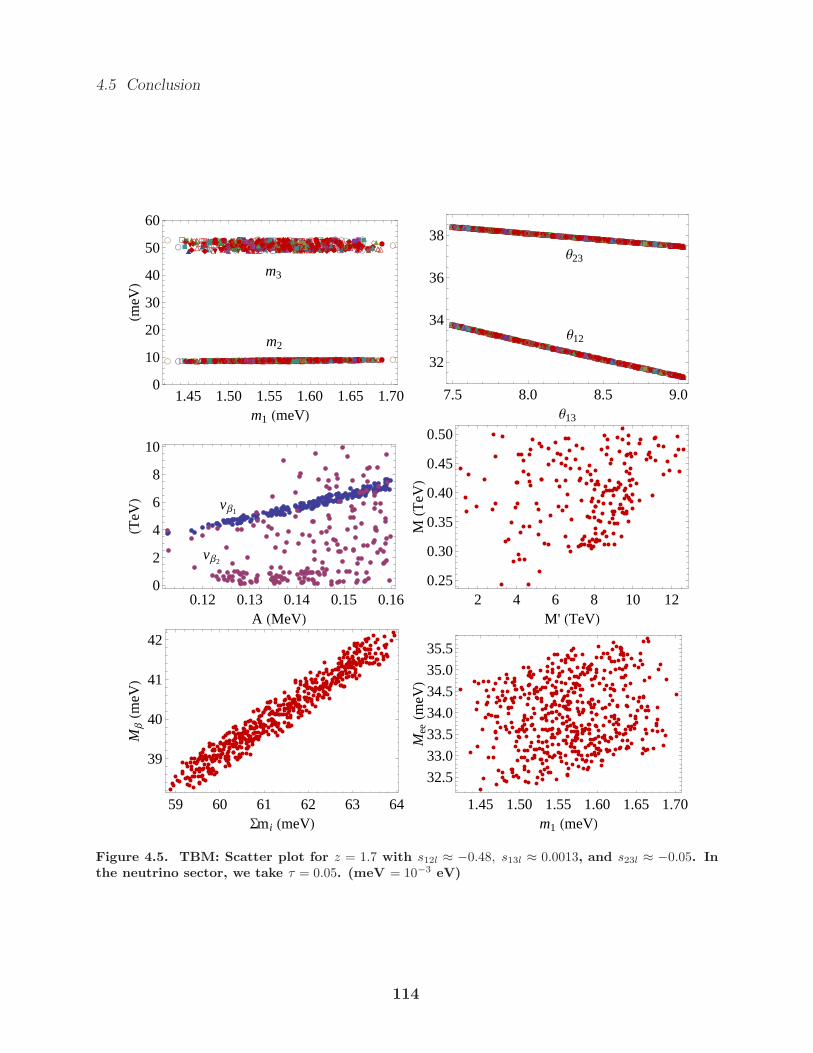
4.5 Conclusion
ì
ì
ì
ì
æ
æ
ì
ì
ó
ó
æ
æ
ò
ò
í
í
à
à
õ
õ
æ
æ
ò
ò
ç
ç
à
à
ó
ó
æ
æ
ì
ì
õ
õ
ç
ç
à
à
ó
ó
ç
ç
í
í
á
á
ç
ç
à
à
á
á
ó
ó
í
í
æ
æ
á
á
á
á
æ
æ
á
á
á
á
à
à
í
í
à
à
ì
ì
æ
æ
à
à
í
í
à
à
æ
æ
ô
ô
ò
ò
ò
ò
ò
ò
ç
ç
à
à
ó
ó
à
à
í
í
æ
æ
ò
ò
ç
ç
ô
ô
ì
ì
á
á
á
á
à
à
à
à
õ
õ
ò
ò
æ
æ
í
í
ò
ò
ç
ç
õ
õ
õ
õ
á
á
á
á
á
á
á
á
á
á
æ
æ
ô
ô
ó
ó
à
à
ô
ô
ô
ô
ì
ì
æ
æ
õ
õ
ô
ô
á
á
ó
ó
ì
ì
ç
ç
í
í
ó
ó
ó
ó
õ
õ
ò
ò
ò
ò
ó
ó
á
á
ó
ó
õ
õ
ç
ç
ò
ò
ì
ì
à
à
à
à
õ
õ
í
í
ó
ó
í
í
ó
ó
æ
æ
ô
ô
ó
ó
ó
ó
á
á
ì
ì
ì
ì
æ
æ
æ
æ
à
à
ô
ô
ó
ó
ô
ô
à
à
à
à
à
à
á
á
ì
ì
í
í
õ
õ
õ
õ
á
á
æ
æ
ì
ì
ì
ì
ô
ô
æ
æ
í
í
ô
ô
ç
ç
õ
õ
ç
ç
õ
õ
ì
ì
ó
ó
ç
ç
á
á
í
í
ì
ì
æ
æ
ì
ì
í
í
á
á
á
á
ô
ô
ò
ò
á
á
á
á
ì
ì
á
á
ì
ì
ì
ì
à
à
ì
ì
í
í
ç
ç
ì
ì
ç
ç
õ
õ
ì
ì
ô
ô
ç
ç
æ
æ
æ
æ
ì
ì
ô
ô
á
á
ç
ç
ì
ì
á
á
ò
ò
æ
æ
ò
ò
í
í
ò
ò
ô
ô
ó
ó
ô
ô
ì
ì
ô
ô
ó
ó
á
á
à
à
á
á
æ
æ
à
à
í
í
ì
ì
á
á
á
á
õ
õ
ò
ò
ç
ç
ó
ó
ó
ó
õ
õ
á
á
ò
ò
ò
ò
ì
ì
ò
ò
ó
ó
õ
õ
ô
ô
ç
ç
ó
ó
à
à
æ
æ
ç
ç
ó
ó
ó
ó
á
á
ò
ò
ì
ì
í
í
ì
ì
à
à
ô
ô
ó
ó
ç
ç
ì
ì
á
á
õ
õ
õ
õ
õ
õ
ì
ì
á
á
ô
ô
á
á
ô
ô
á
á
ó
ó
í
í
ç
ç
ó
ó
à
à
á
á
ô
ô
í
í
ì
ì
à
à
ó
ó
ô
ô
õ
õ
á
á
ò
ò
ó
ó
æ
æ
ó
ó
à
à
õ
õ
ç
ç
í
í
ò
ò
ç
ç
õ
õ
õ
õ
í
í
ô
ô
á
á
ç
ç
í
í
õ
õ
ç
ç
í
í
ì
ì
á
á
æ
æ
à
à
ò
ò
ò
ò
æ
æ
à
à
ç
ç
ô
ô
ó
ó
ç
ç
ì
ì
ì
ì
ô
ô
ò
ò
ó
ó
ç
ç
ô
ô
ô
ô
æ
æ
à
à
õ
õ
æ
æ
ó
ó
õ
õ
í
í
á
á
í
í
ô
ô
ó
ó
í
í
à
à
õ
õ
à
à
á
á
ì
ì
æ
æ
ò
ò
ò
ò
á
á
à
à
ò
ò
ç
ç
à
à
æ
æ
ì
ì
ç
ç
æ
æ
à
à
æ
æ
í
í
ì
ì
ó
ó
í
í
á
á
ì
ì
ç
ç
æ
æ
ç
ç
ì
ì
ò
ò
æ
æ
à
à
õ
õ
ç
ç
ç
ç
ì
ì
õ
õ
ô
ô
ò
ò
ì
ì
í
í
à
à
ç
ç
à
à
õ
õ
ì
ì
ó
ó
í
í
ó
ó
ò
ò
ô
ô
á
á
õ
õ
õ
õ
ì
ì
ç
ç
ó
ó
õ
õ
õ
õ
ò
ò
ô
ô
ç
ç
ì
ì
ô
ô
ç
ç
ì
ì
ó
ó
õ
õ
æ
æ
ó
ó
ò
ò
õ
õ
æ
æ
ó
ó
ç
ç
à
à
æ
æ
ì
ì
õ
õ
æ
æ
à
à
ô
ô
ò
ò
ì
ì
ì
ì
ç
ç
à
à
ì
ì
ô
ô
à
à
á
á
ó
ó
ó
ó
ì
ì
ç
ç
ó
ó
ó
ó
ì
ì
ô
ô
ó
ó
æ
æ
ó
ó
æ
æ
á
á
ç
ç
à
à
í
í
æ
æ
á
á
õ
õ
á
á
à
à
æ
æ
õ
õ
à
à
í
í
ò
ò
õ
õ
õ
õ
ô
ô
á
á
à
à
ó
ó
á
á
à
à
ì
ì
æ
æ
ç
ç
ò
ò
à
à
à
à
ó
ó
ô
ô
ì
ì
à
à
ì
ì
ò
ò
ò
ò
ò
ò
í
í
ç
ç
í
í
ò
ò
æ
æ
õ
õ
õ
õ
ó
ó
í
í
õ
õ
ì
ì
ç
ç
í
í
ì
ì
õ
õ
à
à
õ
õ
ô
ô
ó
ó
í
í
ó
ó
õ
õ
õ
õ
ç
ç
ó
ó
æ
æ
ò
ò
ô
ô
ç
ç
í
í
æ
æ
á
á
æ
æ
æ
æ
ó
ó
ò
ò
ô
ô
à
à
æ
æ
à
à
ì
ì
ì
ì
í
í
ô
ô
ó
ó
ó
ó
æ
æ
ó
ó
ç
ç
ô
ô
à
à
á
á
á
á
õ
õ
ç
ç
õ
õ
à
à
í
í
ì
ì
ô
ô
à
à
ò
ò
ò
ò
á
á
á
á
à
à
ç
ç
æ
æ
ì
ì
á
á
ó
ó
ì
ì
í
í
á
á
õ
õ
ó
ó
í
í
æ
æ
æ
æ
ì
ì
ç
ç
ô
ô
á
á
ì
ì
õ
õ
ç
ç
í
í
ò
ò
ò
ò
ô
ô
à
à
à
à
æ
æ
í
í
ò
ò
ç
ç
ô
ô
à
à
ô
ô
ç
ç
ì
ì
æ
æ
ô
ô
á
á
í
í
æ
æ
í
í
ì
ì
ç
ç
ì
ì
ó
ó
ò
ò
ô
ô
ì
ì
ç
ç
ç
ç
ó
ó
ò
ò
æ
æ
m2
m3
1.45 1.50 1.55 1.60 1.65 1.700
10
20
30
40
50
60
m1 HmeVL
HmeVL
ì
ì
ì
ì
æ
æ
ì
ì
ó
ó
æ
æ
ò
ò
í
í
à
à
õ
õ
æ
æ
ò
ò
ç
ç
à
à
ó
ó
æ
æ
ì
ì
õ
õ
ç
ç
à
à
ó
ó
ç
ç
í
í
á
á
ç
ç
à
à
á
á
ó
ó
í
í
æ
æ
á
á
á
á
æ
æ
á
á
á
á
à
à
í
í
à
à
ì
ì
æ
æ
à
à
í
í
à
à
æ
æ
ô
ô
ò
ò
ò
ò
ò
ò
ç
ç
à
à
ó
ó
à
à
í
í
æ
æ
ò
ò
ç
ç
ô
ô
ì
ì
á
á
á
á
à
à
à
à
õ
õ
ò
ò
æ
æ
í
í
ò
ò
ç
ç
õ
õ
õ
õ
á
á
á
á
á
á
á
á
á
á
æ
æ
ô
ô
ó
ó
à
à
ô
ô
ô
ô
ì
ì
æ
æ
õ
õ
ô
ô
á
á
ó
ó
ì
ì
ç
ç
í
í
ó
ó
ó
ó
õ
õ
ò
ò
ò
ò
ó
ó
á
á
ó
ó
õ
õ
ç
ç
ò
ò
ì
ì
à
à
à
à
õ
õ
í
í
ó
ó
í
í
ó
ó
æ
æ
ô
ô
ó
ó
ó
ó
á
á
ì
ì
ì
ì
æ
æ
æ
æ
à
à
ô
ô
ó
ó
ô
ô
à
à
à
à
à
à
á
á
ì
ì
í
í
õ
õ
õ
õ
á
á
æ
æ
ì
ì
ì
ì
ô
ô
æ
æ
í
í
ô
ô
ç
ç
õ
õ
ç
ç
õ
õ
ì
ì
ó
ó
ç
ç
á
á
í
í
ì
ì
æ
æ
ì
ì
í
í
á
á
á
á
ô
ô
ò
ò
á
á
á
á
ì
ì
á
á
ì
ì
ì
ì
à
à
ì
ì
í
í
ç
ç
ì
ì
ç
ç
õ
õ
ì
ì
ô
ô
ç
ç
æ
æ
æ
æ
ì
ì
ô
ô
á
á
ç
ç
ì
ì
á
á
ò
ò
æ
æ
ò
ò
í
í
ò
ò
ô
ô
ó
ó
ô
ô
ì
ì
ô
ô
ó
ó
á
á
à
à
á
á
æ
æ
à
à
í
í
ì
ì
á
á
á
á
õ
õ
ò
ò
ç
ç
ó
ó
ó
ó
õ
õ
á
á
ò
ò
ò
ò
ì
ì
ò
ò
ó
ó
õ
õ
ô
ô
ç
ç
ó
ó
à
à
æ
æ
ç
ç
ó
ó
ó
ó
á
á
ò
ò
ì
ì
í
í
ì
ì
à
à
ô
ô
ó
ó
ç
ç
ì
ì
á
á
õ
õ
õ
õ
õ
õ
ì
ì
á
á
ô
ô
á
á
ô
ô
á
á
ó
ó
í
í
ç
ç
ó
ó
à
à
á
á
ô
ô
í
í
ì
ì
à
à
ó
ó
ô
ô
õ
õ
á
á
ò
ò
ó
ó
æ
æ
ó
ó
à
à
õ
õ
ç
ç
í
í
ò
ò
ç
ç
õ
õ
õ
õ
í
í
ô
ô
á
á
ç
ç
í
í
õ
õ
ç
ç
í
í
ì
ì
á
á
æ
æ
à
à
ò
ò
ò
ò
æ
æ
à
à
ç
ç
ô
ô
ó
ó
ç
ç
ì
ì
ì
ì
ô
ô
ò
ò
ó
ó
ç
ç
ô
ô
ô
ô
æ
æ
à
à
õ
õ
æ
æ
ó
ó
õ
õ
í
í
á
á
í
í
ô
ô
ó
ó
í
í
à
à
õ
õ
à
à
á
á
ì
ì
æ
æ
ò
ò
ò
ò
á
á
à
à
ò
ò
ç
ç
à
à
æ
æ
ì
ì
ç
ç
æ
æ
à
à
æ
æ
í
í
ì
ì
ó
ó
í
í
á
á
ì
ì
ç
ç
æ
æ
ç
ç
ì
ì
ò
ò
æ
æ
à
à
õ
õ
ç
ç
ç
ç
ì
ì
õ
õ
ô
ô
ò
ò
ì
ì
í
í
à
à
ç
ç
à
à
õ
õ
ì
ì
ó
ó
í
í
ó
ó
ò
ò
ô
ô
á
á
õ
õ
õ
õ
ì
ì
ç
ç
ó
ó
õ
õ
õ
õ
ò
ò
ô
ô
ç
ç
ì
ì
ô
ô
ç
ç
ì
ì
ó
ó
õ
õ
æ
æ
ó
ó
ò
ò
õ
õ
æ
æ
ó
ó
ç
ç
à
à
æ
æ
ì
ì
õ
õ
æ
æ
à
à
ô
ô
ò
ò
ì
ì
ì
ì
ç
ç
à
à
ì
ì
ô
ô
à
à
á
á
ó
ó
ó
ó
ì
ì
ç
ç
ó
ó
ó
ó
ì
ì
ô
ô
ó
ó
æ
æ
ó
ó
æ
æ
á
á
ç
ç
à
à
í
í
æ
æ
á
á
õ
õ
á
á
à
à
æ
æ
õ
õ
à
à
í
í
ò
ò
õ
õ
õ
õ
ô
ô
á
á
à
à
ó
ó
á
á
à
à
ì
ì
æ
æ
ç
ç
ò
ò
à
à
à
à
ó
ó
ô
ô
ì
ì
à
à
ì
ì
ò
ò
ò
ò
ò
ò
í
í
ç
ç
í
í
ò
ò
æ
æ
õ
õ
õ
õ
ó
ó
í
í
õ
õ
ì
ì
ç
ç
í
í
ì
ì
õ
õ
à
à
õ
õ
ô
ô
ó
ó
í
í
ó
ó
õ
õ
õ
õ
ç
ç
ó
ó
æ
æ
ò
ò
ô
ô
ç
ç
í
í
æ
æ
á
á
æ
æ
æ
æ
ó
ó
ò
ò
ô
ô
à
à
æ
æ
à
à
ì
ì
ì
ì
í
í
ô
ô
ó
ó
ó
ó
æ
æ
ó
ó
ç
ç
ô
ô
à
à
á
á
á
á
õ
õ
ç
ç
õ
õ
à
à
í
í
ì
ì
ô
ô
à
à
ò
ò
ò
ò
á
á
á
á
à
à
ç
ç
æ
æ
ì
ì
á
á
ó
ó
ì
ì
í
í
á
á
õ
õ
ó
ó
í
í
æ
æ
æ
æ
ì
ì
ç
ç
ô
ô
á
á
ì
ì
õ
õ
ç
ç
í
í
ò
ò
ò
ò
ô
ô
à
à
à
à
æ
æ
í
í
ò
ò
ç
ç
ô
ô
à
à
ô
ô
ç
ç
ì
ì
æ
æ
ô
ô
á
á
í
í
æ
æ
í
í
ì
ì
ç
ç
ì
ì
ó
ó
ò
ò
ô
ô
ì
ì
ç
ç
ç
ç
ó
ó
ò
ò
æ
æ
Θ23
Θ12
7.5 8.0 8.5 9.0
32
34
36
38
Θ13
vΒ2
vΒ1
0.12 0.13 0.14 0.15 0.160
2
4
6
8
10
A HMeVL
HTeVL
2 4 6 8 10 120.25
0.30
0.35
0.40
0.45
0.50
M' HTeVL
MHT
eVL
59 60 61 62 63 64
39
40
41
42
Smi HmeVL
MΒHm
eVL
1.45 1.50 1.55 1.60 1.65 1.70
32.5
33.0
33.5
34.0
34.5
35.0
35.5
m1 HmeVL
MeeHm
eVL
Figure 4.5. TBM: Scatter plot for z = 1.7 with s12l ≈ −0.48, s13l ≈ 0.0013, and s23l ≈ −0.05. Inthe neutrino sector, we take τ = 0.05. (meV = 10−3 eV)
114
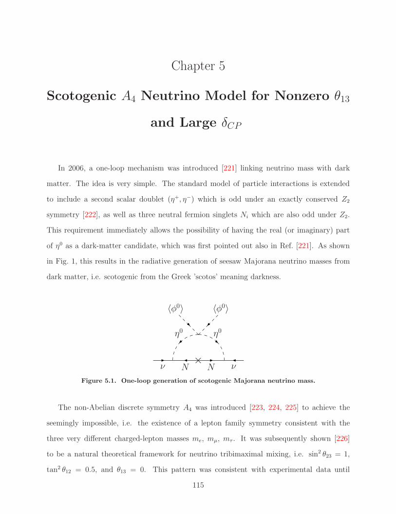
Chapter 5
Scotogenic A4 Neutrino Model for Nonzero θ13
and Large δCP
In 2006, a one-loop mechanism was introduced [221] linking neutrino mass with dark
matter. The idea is very simple. The standard model of particle interactions is extended
to include a second scalar doublet (η+, η−) which is odd under an exactly conserved Z2
symmetry [222], as well as three neutral fermion singlets Ni which are also odd under Z2.
This requirement immediately allows the possibility of having the real (or imaginary) part
of η0 as a dark-matter candidate, which was first pointed out also in Ref. [221]. As shown
in Fig. 1, this results in the radiative generation of seesaw Majorana neutrino masses from
dark matter, i.e. scotogenic from the Greek ’scotos’ meaning darkness.
ν νN N
η0 η0
〈φ0〉 〈φ0〉
×Figure 5.1. One-loop generation of scotogenic Majorana neutrino mass.
The non-Abelian discrete symmetry A4 was introduced [223, 224, 225] to achieve the
seemingly impossible, i.e. the existence of a lepton family symmetry consistent with the
three very different charged-lepton masses me, mµ, mτ . It was subsequently shown [226]
to be a natural theoretical framework for neutrino tribimaximal mixing, i.e. sin2 θ23 = 1,
tan2 θ12 = 0.5, and θ13 = 0. This pattern was consistent with experimental data until
115
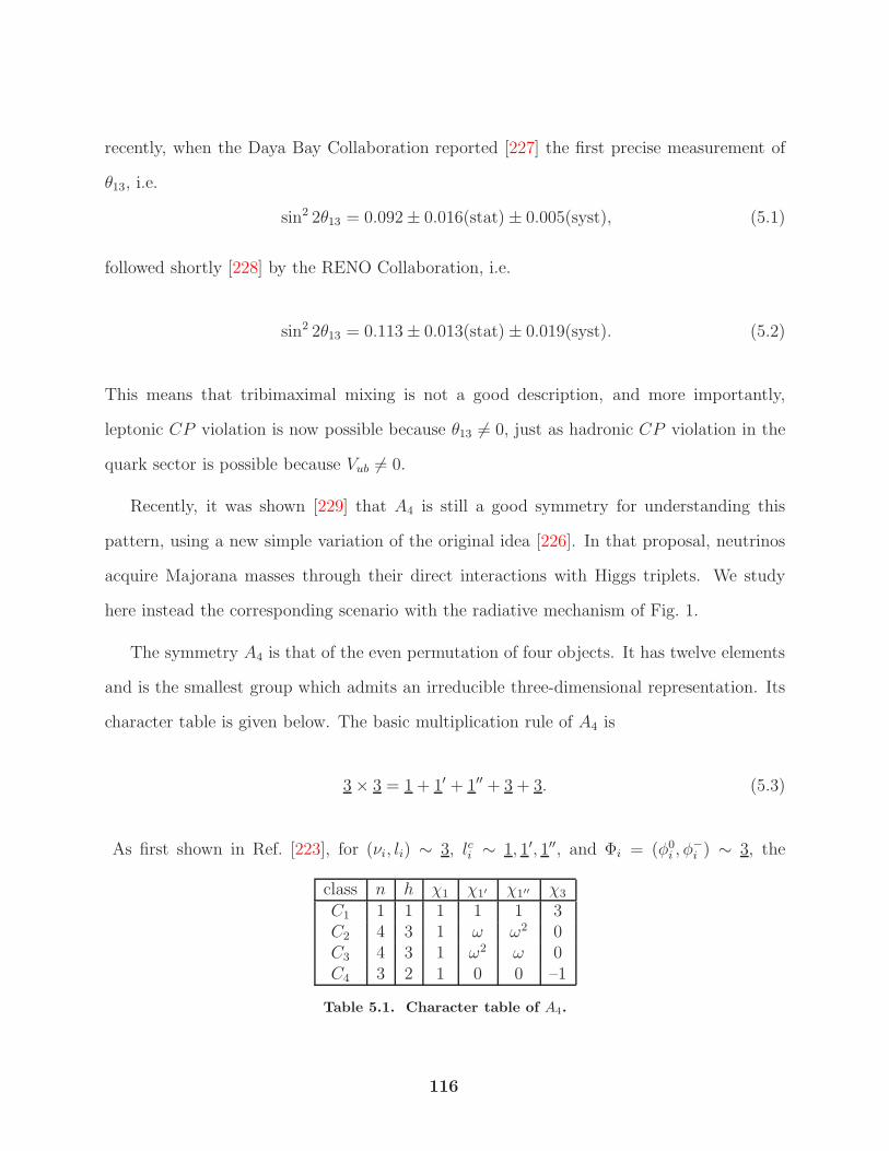
recently, when the Daya Bay Collaboration reported [227] the first precise measurement of
θ13, i.e.
sin2 2θ13 = 0.092± 0.016(stat)± 0.005(syst), (5.1)
followed shortly [228] by the RENO Collaboration, i.e.
sin2 2θ13 = 0.113± 0.013(stat)± 0.019(syst). (5.2)
This means that tribimaximal mixing is not a good description, and more importantly,
leptonic CP violation is now possible because θ13 6= 0, just as hadronic CP violation in the
quark sector is possible because Vub 6= 0.
Recently, it was shown [229] that A4 is still a good symmetry for understanding this
pattern, using a new simple variation of the original idea [226]. In that proposal, neutrinos
acquire Majorana masses through their direct interactions with Higgs triplets. We study
here instead the corresponding scenario with the radiative mechanism of Fig. 1.
The symmetry A4 is that of the even permutation of four objects. It has twelve elements
and is the smallest group which admits an irreducible three-dimensional representation. Its
character table is given below. The basic multiplication rule of A4 is
3× 3 = 1 + 1′ + 1′′ + 3 + 3. (5.3)
As first shown in Ref. [223], for (νi, li) ∼ 3, lci ∼ 1, 1′, 1′′, and Φi = (φ0i , φ
−i ) ∼ 3, the
class n h χ1 χ1′ χ1′′ χ3
C1 1 1 1 1 1 3C2 4 3 1 ω ω2 0C3 4 3 1 ω2 ω 0C4 3 2 1 0 0 –1
Table 5.1. Character table of A4.
116
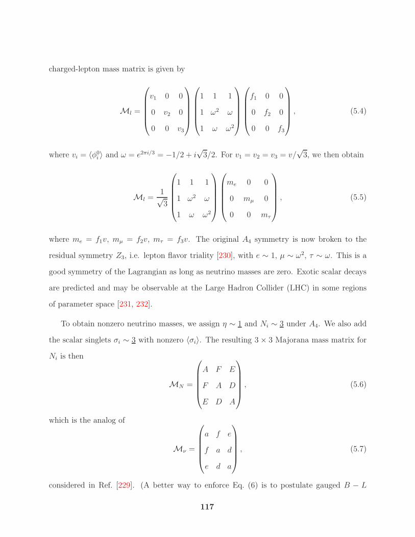
charged-lepton mass matrix is given by
Ml =
v1 0 0
0 v2 0
0 0 v3
1 1 1
1 ω2 ω
1 ω ω2
f1 0 0
0 f2 0
0 0 f3
, (5.4)
where vi = 〈φ0i 〉 and ω = e2πi/3 = −1/2 + i
√3/2. For v1 = v2 = v3 = v/
√3, we then obtain
Ml =1√3
1 1 1
1 ω2 ω
1 ω ω2
me 0 0
0 mµ 0
0 0 mτ
, (5.5)
where me = f1v, mµ = f2v, mτ = f3v. The original A4 symmetry is now broken to the
residual symmetry Z3, i.e. lepton flavor triality [230], with e ∼ 1, µ ∼ ω2, τ ∼ ω. This is a
good symmetry of the Lagrangian as long as neutrino masses are zero. Exotic scalar decays
are predicted and may be observable at the Large Hadron Collider (LHC) in some regions
of parameter space [231, 232].
To obtain nonzero neutrino masses, we assign η ∼ 1 and Ni ∼ 3 under A4. We also add
the scalar singlets σi ∼ 3 with nonzero 〈σi〉. The resulting 3 × 3 Majorana mass matrix for
Ni is then
MN =
A F E
F A D
E D A
, (5.6)
which is the analog of
Mν =
a f e
f a d
e d a
, (5.7)
considered in Ref. [229]. (A better way to enforce Eq. (6) is to postulate gauged B − L
117
and assume complex neutral scalars which transform as 1, 3 under A4, in complete analogy
to the scalar triplets of Ref. [229].) Instead of enforcing E = F = 0 which is required
for tribimaximal mixing, we assume here that F = −E which may be maintained by an
interchange symmetry [226, 233].
Consider now the tribimaximal basis, i.e.
νe
νµ
ντ
=
√2/3 1/
√3 0
−1/√6 1/
√3 −1/
√2
−1/√6 1/
√3 1/
√2
ν1
ν2
ν3
. (5.8)
Since ν1,2,3 are connected to N1,2,3 through the identity matrix, we find
M(1,2,3)N =
A +D 0 0
0 A C
0 C A−D
, (5.9)
where C = (E − F )/√2 =
√2E.
The diagram of Fig. 1 is exactly calculable from the exchange of Re(η0) and Im(η0) and
is given by [221]
(Mν)ij =∑
k
hikhjkMk
16π2
[m2
R
m2R −M2
k
lnm2
R
M2k
− m2I
m2I −M2
k
lnm2
I
M2k
], (5.10)
where∑
k hik(hjk)∗ = |h|2δij , and mR,I are the masses of
√2Re(η0) and
√2Im(η0), respec-
tively. In the limit m2R − m2
I = 2λ5v2 is small compared to m2
0 = (m2R + m2
I)/2, and
m20 << M2
k , Eq. (10) reduces to
(Mν)ij =λ5v
2
8π2
∑
k
hikhjkMk
[lnM2
k
m20
− 1
]. (5.11)
118
In the tribimaximal basis of Eq. (9), we then have
hik = h
1 0 0
0 cos θ − sin θeiφ
0 sin θe−iφ cos θ
eiα′1/2 0 0
0 eiα′2/2 0
0 0 eiα′3/2
, (5.12)
with
cos θ sin θeiφ
− sin θe−iφ cos θ
A C
C A−D
cos θ − sin θe−iφ
sin θeiφ cos θ
=
eiα
′2M2 0
0 eiα′3M3
.
(5.13)
The neutrino mixing matrix U has 4 parameters: s12, s23, s13 and δCP [234]. We choose
the convention Uτ1, Uτ2, Ue3, Uµ3 → −Uτ1,−Uτ2,−Ue3,−Uµ3 to conform with that of the
tribimaximal mixing matrix of Eq. (8), then
M(1,2,3)ν = UT
TBU
eiα1m′1 0 0
0 eiα2m′2 0
0 0 m′3
UTUTB, (5.14)
where m′1,2,3 are the physical neutrino masses, with
m′2 =
√m′
12 +∆m2
21, (5.15)
m′3 =
√m′
12 +∆m2
21/2 + ∆m232 (normal hierarchy), (5.16)
m′3 =
√m′
12 +∆m2
21/2−∆m232 (inverted hierarchy). (5.17)
119
We now diagonalize M(1,2,3)ν using
UǫM(1,2,3)ν UT
ǫ =
eiα′1m′
1 0 0
0 eiα′2m′
2 0
0 0 eiα′3m′
3
, (5.18)
from which we obtain U ′ = UTBUTǫ . To obtain U with the usual convention, we rotate the
phases of the µ and τ rows so that U ′µ3e
−iα′3/2 is real and negative, and U ′
τ3e−iα′
3/2 is real
and positive. These phases are absorbed by the µ and τ leptons and are unobservable. We
then rotate the ν1,2 columns so that U ′e1e
−iα′3/2 = Ue1e
iα′′1/2 and U ′
e2e−iα′
3/2 = Ue2eiα′′
2/2, where
Ue1 and Ue2 are real and positive. The physical relative Majorana phases of ν1,2 are then
α1,2 = α′1,2 + α′′
1,2. The three angles and the Dirac phase are extracted according to
tan2 θ12 = |U ′e2/U
′e1|2, tan2 θ23 = |U ′
µ3/U′τ3|2, sin θ13e
−iδCP = U ′e3e
−iα′3/2. (5.19)
The effective Majorana neutrino mass in neutrinoless double beta decay is then given by
mee = |U2e1e
iα1m′1 + U2
e2eiα2m′
2 + U2e3m
′3|. (5.20)
In Eq. (9), let A be real and positive by convention, then both C and D may be complex,
i.e. C = CR + iCI and D = DR + iDI . The 2 × 2 matrix of Eq. (13) can be solved exactly
to yield
tanφ =CRDI − CIDR
CR(2A−DR)− CIDI, (5.21)
tan 2θ =2[4A2C2
R − 4ACR(CRDR + CIDI) + (C2R + C2
I )(D2R +D2
I )]1/2
2ADR − (D2R +D2
I ), (5.22)
120
with
eiα′2M2 = cos2 θA + 2 sin θ cos θeiφC + sin2 θe2iφ(A−D), (5.23)
eiα′3M3 = cos2 θ(A−D)− 2 sin θ cos θe−iφC + sin2 θe−2iφA. (5.24)
The corresponding U ′ elements are
U ′e1 =
√2
3, U ′
e2 =cos θ√
3, U ′
e3 = −sin θ√3e−iφ, (5.25)
U ′µ3 = −cos θ√
2− sin θ√
3e−iφ, U ′
τ3 =cos θ√
2− sin θ√
3e−iφ. (5.26)
If we absorb the scale factor λ5h2v2/8π2 into the parameters A,C,D as well as m0, then
the mass eigenvalues of Eq. (11) are given by
m′k =
1
Mk
[lnM2
k
m20
− 1
], (5.27)
which are the ones used in Eqs. (14) and (18). Since m0 is an unknown, having to do with
the dark-matter scalar mass, we fix it by requiring M1/m0 = 10, where M1 = |A+D|. If we
input the five parameters A,CR, CI , DR, DI , we will obtain m′1,2,3 as well as the three mixing
angles and the three CP phases. For our numerical analysis, we set
∆m221 = 7.59× 10⁻⁵ eV2, ∆m2
32 = 2.45× 10⁻³ eV2, (5.28)
and vary θ13 in the range
sin2 2θ13 = 0.05 to 0.15. (5.29)
Following Ref. [229], we look for solutions with sin2 2θ23 = 0.92 and 0.96. Whereas only
normal hierarchy is allowed in the model of Ref. [229], we find solutions for both normal and
inverted hierarchies, as well as quasi-degenerate solutions, as detailed below.
121
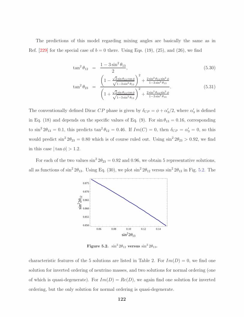
The predictions of this model regarding mixing angles are basically the same as in
Ref. [229] for the special case of b = 0 there. Using Eqs. (19), (25), and (26), we find
tan2 θ12 =1− 3 sin2 θ13
2, (5.30)
tan2 θ23 =
(1−
√2 sin θ13 cosφ√1−3 sin2 θ13
)2
+ 2 sin2 θ13 sin2 φ1−3 sin2 θ13
(1 +
√2 sin θ13 cosφ√1−3 sin2 θ13
)2
+ 2 sin2 θ13 sin2 φ1−3 sin2 θ13
. (5.31)
The conventionally defined Dirac CP phase is given by δCP = φ+α′3/2, where α
′3 is defined
in Eq. (18) and depends on the specific values of Eq. (9). For sin θ13 = 0.16, corresponding
to sin2 2θ13 = 0.1, this predicts tan2 θ12 = 0.46. If Im(C) = 0, then δCP = α′3 = 0, so this
would predict sin2 2θ23 = 0.80 which is of course ruled out. Using sin2 2θ23 > 0.92, we find
in this case | tanφ| > 1.2.
For each of the two values sin2 2θ23 = 0.92 and 0.96, we obtain 5 representative solutions,
all as functions of sin2 2θ13. Using Eq. (30), we plot sin2 2θ12 versus sin2 2θ13 in Fig. 5.2. The
0.06 0.08 0.10 0.12 0.140.850
0.855
0.860
0.865
0.870
0.875
sin22Θ13
sin2 2Θ
12
Figure 5.2. sin2 2θ12 versus sin2 2θ13.
characteristic features of the 5 solutions are listed in Table 2. For Im(D) = 0, we find one
solution for inverted ordering of neutrino masses, and two solutions for normal ordering (one
of which is quasi-degenerate). For Im(D) = Re(D), we again find one solution for inverted
ordering, but the only solution for normal ordering is quasi-degenerate.
122
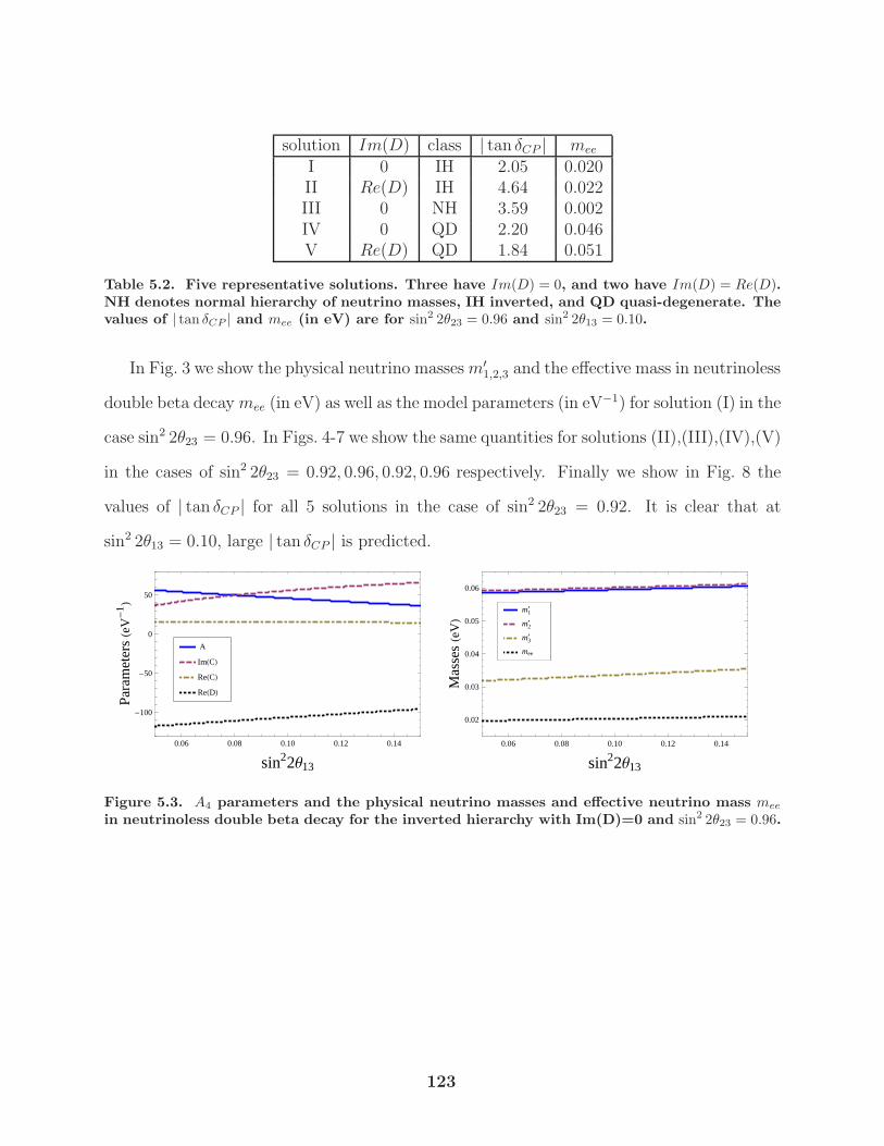
solution Im(D) class | tan δCP | mee
I 0 IH 2.05 0.020II Re(D) IH 4.64 0.022III 0 NH 3.59 0.002IV 0 QD 2.20 0.046V Re(D) QD 1.84 0.051
Table 5.2. Five representative solutions. Three have Im(D) = 0, and two have Im(D) = Re(D).NH denotes normal hierarchy of neutrino masses, IH inverted, and QD quasi-degenerate. Thevalues of | tan δCP | and mee (in eV) are for sin2 2θ23 = 0.96 and sin2 2θ13 = 0.10.
In Fig. 3 we show the physical neutrino massesm′1,2,3 and the effective mass in neutrinoless
double beta decaymee (in eV) as well as the model parameters (in eV−1) for solution (I) in the
case sin2 2θ23 = 0.96. In Figs. 4-7 we show the same quantities for solutions (II),(III),(IV),(V)
in the cases of sin2 2θ23 = 0.92, 0.96, 0.92, 0.96 respectively. Finally we show in Fig. 8 the
values of | tan δCP | for all 5 solutions in the case of sin2 2θ23 = 0.92. It is clear that at
sin2 2θ13 = 0.10, large | tan δCP | is predicted.
0.06 0.08 0.10 0.12 0.14
-100
-50
0
50
sin22Θ13
Par
amet
ersHe
V-
1 L
ReHDL
ReHCL
ImHCL
A
0.06 0.08 0.10 0.12 0.14
0.02
0.03
0.04
0.05
0.06
sin22Θ13
Mas
sesHe
VL
mee
m3¢
m2¢
m1¢
Figure 5.3. A4 parameters and the physical neutrino masses and effective neutrino mass mee
in neutrinoless double beta decay for the inverted hierarchy with Im(D)=0 and sin2 2θ23 = 0.96.
123
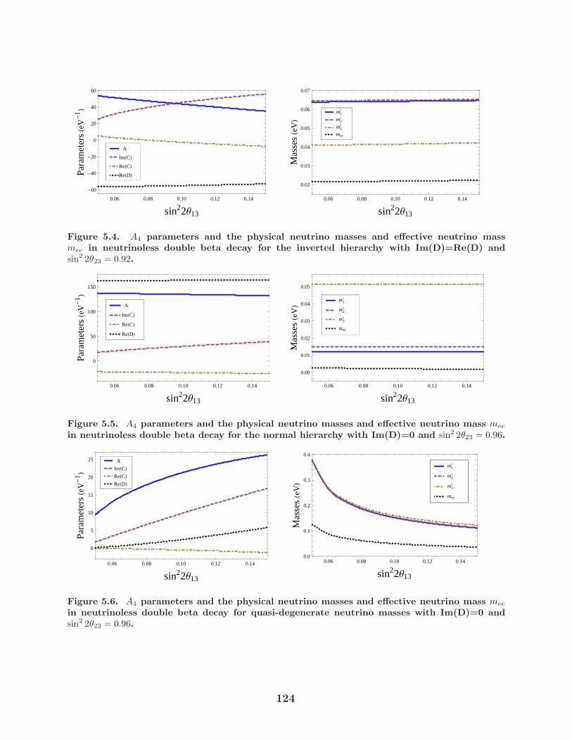
0.06 0.08 0.10 0.12 0.14
-60
-40
-20
0
20
40
60
sin22Θ13
Par
amet
ersHe
V-
1 L
ReHDL
ReHCL
ImHCL
A
0.06 0.08 0.10 0.12 0.14
0.02
0.03
0.04
0.05
0.06
0.07
sin22Θ13
Mas
sesHe
VL
mee
m3¢
m2¢
m1¢
Figure 5.4. A4 parameters and the physical neutrino masses and effective neutrino massmee in neutrinoless double beta decay for the inverted hierarchy with Im(D)=Re(D) andsin2 2θ23 = 0.92.
0.06 0.08 0.10 0.12 0.14
0
50
100
150
sin22Θ13
Par
amet
ersHe
V-
1 L
ReHDL
ReHCL
ImHCL
A
0.06 0.08 0.10 0.12 0.14
0.00
0.01
0.02
0.03
0.04
0.05
sin22Θ13
Mas
sesHe
VL
mee
m3¢
m2¢
m1¢
Figure 5.5. A4 parameters and the physical neutrino masses and effective neutrino mass mee
in neutrinoless double beta decay for the normal hierarchy with Im(D)=0 and sin2 2θ23 = 0.96.
0.06 0.08 0.10 0.12 0.14
0
5
10
15
20
25
sin22Θ13
Par
amet
ersHe
V-
1 L
ReHDL
ReHCL
ImHCL
A
0.06 0.08 0.10 0.12 0.140.0
0.1
0.2
0.3
0.4
sin22Θ13
Mas
sesHe
VL
mee
m3¢
m2¢
m1¢
Figure 5.6. A4 parameters and the physical neutrino masses and effective neutrino mass mee
in neutrinoless double beta decay for quasi-degenerate neutrino masses with Im(D)=0 andsin2 2θ23 = 0.96.
124
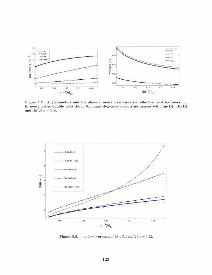
0.06 0.08 0.10 0.12 0.14
0
5
10
15
20
25
30
sin22Θ13
Par
amet
ersHe
V-
1 L
ReHDL
ReHCL
ImHCL
A
0.06 0.08 0.10 0.12 0.14
0.05
0.10
0.15
0.20
sin22Θ13
Mas
sesHe
VL
mee
m3¢
m2¢
m1¢
Figure 5.7. A4 parameters and the physical neutrino masses and effective neutrino mass mee
in neutrinoless double beta decay for quasi-degenerate neutrino masses with Im(D)=Re(D)and sin2 2θ23 = 0.96.
0.06 0.08 0.10 0.12 0.14
1
2
3
4
5
sin22Θ13
Ètan∆
CPÈ
QD, ImHDL=ReHDL
QD, ImHDL=0
NH, ImHDL=0
IH, ImHDL=ReHDL
IH, ImHDL=0
Figure 5.8. | tan δCP | versus sin2 2θ13 for sin2 2θ23 = 0.92.
125
Chapter 6
Radiative Scaling Neutrino Mass with A4
Symmetry
The origin of neutrino mass is the topic of many theoretical discussions. The consensus
is that its smallness is due to some mass scale larger than the electroweak breaking scale of
about 100 GeV. If there are no particles beyond those of the standard model lighter than
this scale, then the well-known unique dimension-five opeartor [235]
L5 =−fij2Λ
(νiφ0 − liφ
+)(νjφ0 − ljφ
+) +H.c. (6.1)
induces Majorana neutrino masses as the Higgs scalar φ0 acquires a nonzero vacuum expec-
tation value 〈φ0〉 = v, so that
(Mν)ij =fijv
2
Λ. (6.2)
This shows that neutrino mass is seesaw in character, i.e. it is inversely proportional to
some large scale Λ. The ultraviolet completion of this effective operator may be accom-
plished in three ways at tree level [236] using (I) heavy Majorana fermion singlets Ni, (II)
a heavy scalar triplet (ξ++, ξ+, ξ0), or (III) heavy Majorana fermion triplets (Σ+,Σ0,Σ0)i,
commonly referred to as Type I, Type II, or Type III seesaw. There are also three one-
particle-irreducible (1PI) one-loop realizations [236]. Recently the one-particle-reducible
(1PR) diagrams have also been considered [237].
If there are new particles with masses below the elctroweak scale, such as fermion singlets
νS with mass mS, then neutrinos may acquire mass through their mixing with νS. However,
this mechanism is still seesaw because mν is still inversely proportional to mS. There is
126
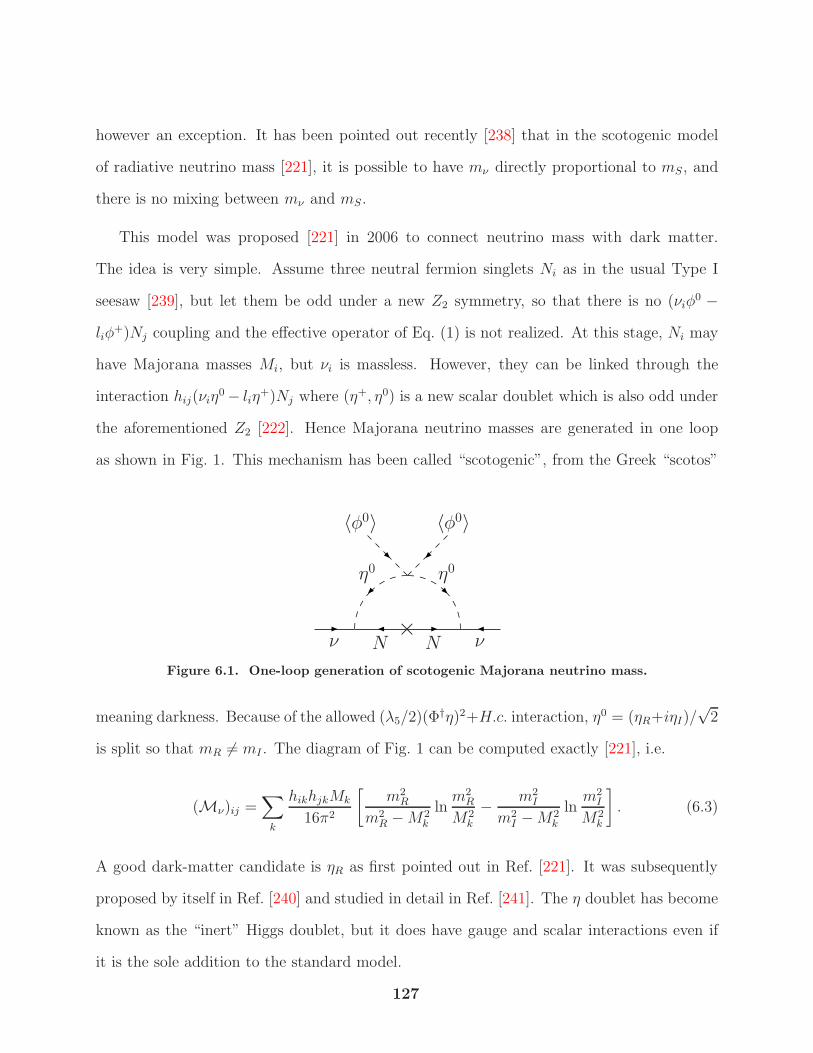
however an exception. It has been pointed out recently [238] that in the scotogenic model
of radiative neutrino mass [221], it is possible to have mν directly proportional to mS, and
there is no mixing between mν and mS.
This model was proposed [221] in 2006 to connect neutrino mass with dark matter.
The idea is very simple. Assume three neutral fermion singlets Ni as in the usual Type I
seesaw [239], but let them be odd under a new Z2 symmetry, so that there is no (νiφ0 −
liφ+)Nj coupling and the effective operator of Eq. (1) is not realized. At this stage, Ni may
have Majorana masses Mi, but νi is massless. However, they can be linked through the
interaction hij(νiη0− liη
+)Nj where (η+, η0) is a new scalar doublet which is also odd under
the aforementioned Z2 [222]. Hence Majorana neutrino masses are generated in one loop
as shown in Fig. 1. This mechanism has been called “scotogenic”, from the Greek “scotos”
ν νN N
η0 η0
〈φ0〉 〈φ0〉
×Figure 6.1. One-loop generation of scotogenic Majorana neutrino mass.
meaning darkness. Because of the allowed (λ5/2)(Φ†η)2+H.c. interaction, η0 = (ηR+iηI)/
√2
is split so that mR 6= mI . The diagram of Fig. 1 can be computed exactly [221], i.e.
(Mν)ij =∑
k
hikhjkMk
16π2
[m2
R
m2R −M2
k
lnm2
R
M2k
− m2I
m2I −M2
k
lnm2
I
M2k
]. (6.3)
A good dark-matter candidate is ηR as first pointed out in Ref. [221]. It was subsequently
proposed by itself in Ref. [240] and studied in detail in Ref. [241]. The η doublet has become
known as the “inert” Higgs doublet, but it does have gauge and scalar interactions even if
it is the sole addition to the standard model.
127
The usual assumption for neutrino mass in Eq. (1) is
m2I −m2
R << m2I +m2
R << M2k , (6.4)
in which case
(Mν)ij =λ5v
2
8π2
∑
k
hikhjkMk
[lnM2
k
m20
− 1
], (6.5)
where m20 = (m2
I +m2R)/2 and m2
R −m2I = 2λ5v
2 (v = 〈φ0〉). This scenario is often referred
to as the radiative seesaw. What was not realized in most applications of this model since
2006 is that there is another very interesting scenario, i.e.
M2k << m2
R, m2I . (6.6)
Neutrino masses are then given by [238]
(Mν)ij =ln(m2
R/m2I)
16π2
∑
k
hikhjkMk. (6.7)
This simple expression is actually very extraordinary, because neutrino mass is now not
inversely proportional to some large scale. In that case, how do we understand the smallness
ofmν? The answer is lepton number. In this model, (ν, l)i have lepton number L = 1 and Nk
have L = −1, and L is conserved in all interactions except for the Majorana mass terms Mk
which break L to (−1)L. We may thus argue that Mk should be small compared to all other
mass terms which conserve L, the smallest of which is the electron mass, me = 0.511 MeV. It
is thus reasonable to have Mk ∼ 10 keV, in which case mν ∼ 0.1 eV is obtained if h2 ∼ 10−3
in Eq. (7). Each neutrino mass is then simply proportional to a linear combination of Mk
according to Eq. (7). Their ratio is just a scale factor and small neutrino masses are due to
this “scaling” mechanism. Note that the interesting special case where only M1 is small has
been considered previously [242, 243]. Note also that if |m2I −m2
R| = 2|λ5|v2 << |m2I +m2
R|,
128
then ln(m2R/m
2I) would be strongly suppressed, but this is not compulsory. For example, let
mR = 240 GeV, mI = 150 GeV, then |λ5| = 0.58 and ln(m2R/m
2I) = 0.94.
The scotogenic model [221] with largeMk, i.e. Eq. (5), has been extended recently [244] to
include the well-known non-Abelian discrete symmetry A4 [223, 224, 225]. Here we consider
the case of Eq. (7). This assumption changes the phenomenology of Nk as well as (η+, η0)
and may render this model to be more easily verifiable at the Large Hadron Collider (LHC).
We let (η+, η0) be a singlet under A4 and both (νi, li) and Nk to be triplets. In that case,
hik = hδik, (6.8)
and
Mν = ζMN , (6.9)
where ζ = h2 ln(m2R/m
2I)/16π
2 is the scale factor. The soft breaking of A4 which shapes MN
is then directly transmitted to Mν .
One immediate consequence of this restricted scaling mechanism for neutrino mass is
that if M1,2,3 are all of order 10 keV, then the three neutrino masses are all of order 0.1 eV,
i.e. a quasidegenerate scenario. For example, if m1 = 0.1 eV and is the lightest, then for
M1 = 10 keV, M3 = 105(m1 +√
∆m231) = 14.85 keV. Another immediate consequence is
that the interactions of N1,2,3 with the charged leptons through η+ depend only on h and the
mismatch between the charged-lepton mass matrix and the neutrino mass matrix, i.e. the
experimentally determined neutrino mixing matrix Ulν . Hence µ → eγ is highly suppressed
because the leading term of its amplitude is proportional to∑
k hµkh∗ek = |h|2
∑k UµkU
∗ek = 0.
The next term∑
k UµkU∗ekM
2k/m
2η+ is nonzero but is negligibly small. This means that there
is no useful bound on the η+ mass from µ → eγ. Note that A4 may be replaced by any
other flavor symmetry as long as it is possible to have Eq. (8) using the singlet and triplet
representations of that symmetry. As for the muon anomalous magnetic moment, it is given
129
by [245]
∆aµ = −m2
µ|h|296π2m2
η+= −1.18× 10⁻¹²
( |h|210−3
)(100 GeV
mη+
)2
. (6.10)
Since the experimental uncertaintly is 6× 10⁻¹⁰, this also does not give any useful bound on
the η+ mass.
If η±, ηR, ηI are of order 102 GeV, the interactions of Nk with the neutrinos and charged
leptons are weaker than the usual weak interaction, hence Nk may be considered “sterile” and
become excellent warm dark-matter candidates [246, 247]. However, unlike the usual sterile
neutrinos [248] which mix with the active neutrinos, the lightest Nk here is absolutely stable.
This removes one of the most stringent astrophysical constraints on warm dark matter, i.e.
the absence of galactic X-ray emission from its decay, which would put an upper bound of
perhaps 2.2 keV on its mass [249], whereas Lyman-α forest observations (which still apply
in this case) impose a lower bound of perhaps 5.6 keV [250]. Such a stable sterile neutrino
(called a “scotino”) is also possible in an unusual left-right extension [251] of the standard
model. Conventional left-right models where the SU(2)R neutrinos mix with the SU(2)L
neutrinos have also been studied [252, 253, 254].
Since Nk are assumed light, muon decay proceeds at tree level through η+ exchange, i.e.
µ→ NµeNe. The inclusive rate is easily calculated to be
Γ(µ → NµeNe) =|h|4m5
µ
6144π3m4η+. (6.11)
Since Nµ and Ne are invisible just as νµ and νe are invisible in the dominant decay µ →
νµeνe (with rate G2Fm
5µ/192π
3), this would change the experimental value of GF . Using the
experimental uncertainty of 10−5 in the determination of GF , we find
mη+ > 70 GeV (6.12)
130
for |h|2 = 10−3. This is a useful bound on the η+ mass, but it is also small enough so that η+
may be observable at the LHC. The phenomenological bound on mη+ from e+e− production
at LEPII has been estimated [255] to be 70 – 90 GeV. A bound of 80 GeV was used in a
previous study [256] of this model.
Whereas the lightest scotino, say N1, is absolutely stable, N2,3 will decay into N1 through
ηR and ηI . The decay rate of N3 → N1ν1ν3 is given by
Γ(N3 → N1ν1ν3) =|h|4
256π3M3
(1
m2R
+1
m2I
)2
×(M6
3
96− M2
1M43
12+M6
1
12− M8
1
96M23
+M4
1M23
8lnM2
3
M21
). (6.13)
Let M1 = 10 keV, M3 = 14.85 keV, |h|2 = 10−3, mR = 240 GeV, mI = 150 GeV, then this
rate is 1.0×10−46 GeV, corresponding to a lifetime of 2.1×10¹⁴ y, which is much longer than
the age of the Universe of 13.75 ± 0.11 × 10⁹ y. The lifetime of N2 is even longer because
∆m221 << ∆m2
31. Hence both N2 and N3 are stable enough to be components of warm dark
matter. However, N2,3 → N1γ are negligible for the same reason that µ → eγ is negligible,
so they again have no galactic X-ray signatures.
Since η+ may be as light as 70 GeV, it may be observable at the LHC. Assuming that the
recently observed particle [257, 258] at the LHC is the Higgs boson H coming from (φ+, φ0),
the decay H → η+η− is not allowed for mH = 126 GeV. However, η± will contribute to the
H → γγ rate, as already pointed out [259, 260, 261, 262]. What sets our model apart is
the inclusive decay of η± → l±N1,2,3, which is of universal strength. At the LHC, the pair
production of η+η− will then lead to l+i l−j final states with equal probability for each flavor
combination. For example, e+µ− and µ+e− will each occur 1/9 of the time. This signature
together with the large missing energy of N1,2,3 may allow it to be observed at the LHC.
However, these events also come from W+W− production and their subsequent leptonic
decays. If data show an excess of such events [263] over the standard-model prediction, it
131
could be due to η+η−, but it may also simply come from an incorrect scale factor used in
the standard-model calculation.
In the supersymmetric SU(5) completion [264] of this model, there are exotic quarks
which may be produced abundantly. Their decays into η± would have four leptons of different
flavor in the final state. This may be a better signature of this model. Details will be given
elsewhere.
In conclusion, the scotogenic model [221] of neutrino mass with a solution [238] where
there is no seesaw mechanism and N1,2,3 have masses of order 10 keV has been implemented
with the non-Abelian discrete symmetry A4. The scotinos N1,2,3 are good warm dark-matter
candidates which can explain the structure of the Universe at all scales [246, 247]. Since N1 is
absolutely stable and the decays N2,3 → N1γ are negligible, the galactic X-ray upper bound
of perhaps 2.2 keV on its mass [249] is avoided. It will also not be detected in terrestrial
experiments. On the other hand, since this model requires an extra scalar doublet, and η±
may be as light as 70 GeV, it may be tested at the LHC, especially if it is the decay product
of an exotic quark.
132
Chapter 7
Nonstandard interactions of tau neutrino via
charged Higgs and W ′ contribution
7.1 Introduction
It has been established that NSI cannot be an explanation for the standard oscillation phe-
nomena, but it may be present as a subleading effect. Many NSI involve flavor changing
neutral current or charged current lepton flavor violating processes. In this work we con-
sider charged current interactions involving a charged Higgs and a W ′ gauge boson in the
tau-neutrino nucleon scattering as categorized according the value of the invariant mass into
three subprocesses; quasielastic scattering processes ντ + n→ τ− + p and ντ + p→ τ+ + n,
∆-Resonance production ντ + n → τ− + ∆+ and ντ + p → τ+ + ∆0, and deep inelastic
scattering ντ +N → τ−+X and ντ +N → τ++X . In neutrino experiments, to measure the
mixing angle the neutrino-nucleus interaction is assumed to be SM-like. If there is a charged
Higgs or a W ′ contribution to this interaction, then there will be an error in the extracted
mixing angle. We will calculate the error in the extracted mixing angle.
The reaction ντ + N → τ− + X is relevant for experiments like Super-Kamiokande
(Super-K) [265, 266] and OPERA [267] that seek to measure νµ → ντ oscillation by the
observation of the τ lepton . The above interaction is also important for the DONuT ex-
periment [268] which measured the charged-current (CC) interaction cross section of the tau
neutrino. The DONuT central-value results for a ντ scattering cross section show deviation
from the standard model predictions by about 40% but with large experimental errors; thus,
the measurements are consistent with the standard model. The new physics (NP) effects
133
7.1 Introduction
calculated in this work modify the SM cross sections by less than 10% and are therefore
consistent with the DONuT measurements. There have been recent measurements of the
appearance of atmospheric tau neutrinos by Super-K [265] and by the OPERA Collaboration
[267].
The reactor neutrino experiments such as Double Chooz [269], Daya Bay [270], and RENO
[271] measure the mixing angle θ13 from the survival probability of an electron antineutrino,
P( νe → νe). If high-energy Long Base Line (LBL) experiments (or atmospheric neutrino
experiments scanning in the multi-GeV neutrino energy range) could measure θ13 via ντ
appearance then the NP effects in ντ +N → τ− +X and ντ +N → τ+ +X would impact
the θ13 measurement and a mismatch between this measurement and that performed at the
reactors could be a hint of a NSI in the former.
Generally, neutrino scattering contains contributions from various processes such as
quasielastic scattering (QE), resonance scattering (RES), and deep inelastic scattering (DIS).
Just above the threshold energy for τ production, which is 3.45 GeV [265, 266], the quasielas-
tic interaction dominates in ντ scattering [272, 273]. At higher scattering energies other pro-
cesses have to be included. For instance, the DIS is expected to be dominant above around 10
GeV [273], and so ντ scattering at the OPERA experiment, running at the average neutrino
energy Eν = 17 GeV [267], will be dominated by DIS.
There are several reasons to consider NSI involving the (ντ , τ) sector. First, the third
generation may be more sensitive to new physics effects because of their larger masses. As
an example, in certain versions of the two Higgs doublet models (2HDM) the couplings of
the new Higgs bosons are proportional to the masses, and so new physics effects are more
pronounced for the third generation. Second, the constraints on NP involving the third gen-
eration leptons are somewhat weaker, allowing for larger new physics effects. Interestingly,
the branching ratio of B decays to τ final states shows some tension with the SM predictions
[275, 276] and this could indicate NP, possibly in the scalar or gauge boson sector [277].
134
7.1 Introduction
Some examples of work that deals with NSI at the detector, though not necessarily involving
the third family leptons, can be found in Refs. [278, 279, 280].
If there is NP involving the third generation leptons, one can search for it in B decays
such as B → τντ , B → D(∗)τντ [281], b → sτ+τ− etc. In general, the NP interaction in B
decays may not be related to the one in ντ + n→ τ− + p and ντ + p→ τ+ + n, and so these
scattering processes probe different NP. The same NP in ντ+n→ τ−+p and ντ+p→ τ++n
can be probed in τ decays [282], and we will consider the constraint on NP from this decay.
However, in general, the scattering and the decay processes probe NP in different energy
regions.
The form of NP in ντ +N → τ−+X involves the operator ONP = uΓidτΓjντ , where Γi,j
are some Dirac structures. The process ντ + N → τ+ + X gets a contribution from O†NP .
We will assume CP conserving NP in this work, and so the coefficients of the NP operators
are real. The same NP operator can also contribute to hadronic tau decays τ− → π−ντ and
τ− → ρ−ντ , and the measured branching ratio of these decays can be used to constrain the
couplings in the operator ONP . The ratio of the charged Higgs contribution to the SM in
ντ + N → τ− + X and ντ + N → τ+ + X is roughly (mN/mπ) larger compared to the
same ratio in τ− → π−ντ , where mN,π are the nucleon and pion masses. Hence, significant
charged Higgs effects are possible in ντ + N → τ− + X and ντ + N → τ+ + X even after
imposing constraints from τ decays. We note that new interactions in the up and down quark
sectors can be constrained if one assumes CKM unitarity. However, we do not consider this
constraint as the NP in ONP involves contributions from both the quark and the lepton
sectors.
As noted above, at the quark level NSI in ντ + N → τ− + X and ντ + N → τ+ + X
involve the u and the d quarks. Often in the analysis of NSI, hadronization effects of the
quarks via form factors are not included. As we show in our calculation the form factors
play an important role in the energy dependence of the NP effects. In an accurate analysis
135
7.2 Model-independent analysis of new physics
one should also include nuclear physics effects which take into account the fact that the
neutron and the proton are not free but bound in the nucleus. There is a certain amount of
model dependence in this part of the analysis [283], and therefore we will not include nuclear
effects in our calculation. Such effects can be easily incorporated once the free scattering
cross sections are known.
This work is organized in the following way. In the next section, we present a model-
independent analysis of NP effects. Then we discuss the kinematics of the interaction. In
the following three sections, we consider charged Higgs and W ′ effects to the three pro-
cesses quasi-elastic interaction, ∆ resonance production and deep inelastic scattering in the
neutrino-nucleon interactions ντ +N → τ− +X and ντ +N → τ+ +X . In the last section,
we present our conclusions.
7.2 Model-independent analysis of new physics
The process ντ +N → τ−+X will impact the measurement of the oscillation probability for
the νµ → ντ transition and hence the extraction of the mixing angle θ23. The measurement
of the atmospheric mixing angle θ23 relies on the following relationship [284]:
N(ντ ) = P (νµ → ντ )× Φ(νµ)× σSM(ντ ) , (7.1)
where N(ντ ) is the number of observed events, Φ(νµ) is the flux of muon neutrinos at the
detector, σSM(ντ ) is the total cross section of tau neutrino interactions with nucleons in the
SM at the detector, and P (νµ → ντ ) is the probability for the flavor transition νµ → ντ .
This probability is a function of (E, L, ∆m2ij , θij) with i, j = 1, 2, 3, where ∆m2
ij is the
squared-mass difference, θij is the mixing angle, E is the energy of neutrinos, and L is the
136
7.2 Model-independent analysis of new physics
distance traveled by neutrinos. The dominant term of the probability is
P (νµ → ντ ) ≈ sin2 2θ23 cos4 θ13 sin
2(∆m223L/4E). (7.2)
In the presence of NP, Eq. 7.1 is modified as
N(ντ ) = P (νµ → ντ )× Φ(νµ)× σtot(ντ ), (7.3)
with σtot(ντ ) = σSM(ντ ) + σNP(ντ ), where σNP(ντ ) refers to the additional terms of the SM
contribution towards the total cross section. Hence, σNP(ντ ) includes contributions from
both the SM and NP interference amplitudes, and the pure NP amplitude. From Eqs. (7.1,
7.3), assuming θ13 to be small,1
sin2 2(θ23) = sin2 2(θ23)SM1
1 + r23, (7.4)
where θ23 = (θ23)SM + δ23 is the actual atmospheric mixing angle, whereas (θ23)SM is the
extracted mixing angle assuming the SM ντ scattering cross section. Assuming negligible
new physics effects in the µ−N interaction, the actual mixing angle θ23 is the same as the
mixing angle extracted from the survival probability P (νµ → νµ) measurement. We will take
the best-fit value for the mixing angle to be given by θ23 = 42.8 [285]. In other words, the
presence of new physics in a ντ -nucleon scattering will result in the mixing angle, extracted
from a ντ appearance experiment, being different than the mixing angle from νµ survival
probability measurements. The relationship between the ratio of the NP contribution to the
SM cross section r23 = σNP (ντ )/σSM(ντ ) and δ23 can be expressed in a model-independent
1The presence of NP impacts the extraction of the combination sin2 2θ23 cos4 θ13. The NP changes the
extracted value of θ23 as well as θ13. But we fix the value of θ13 as an input at this point.
137
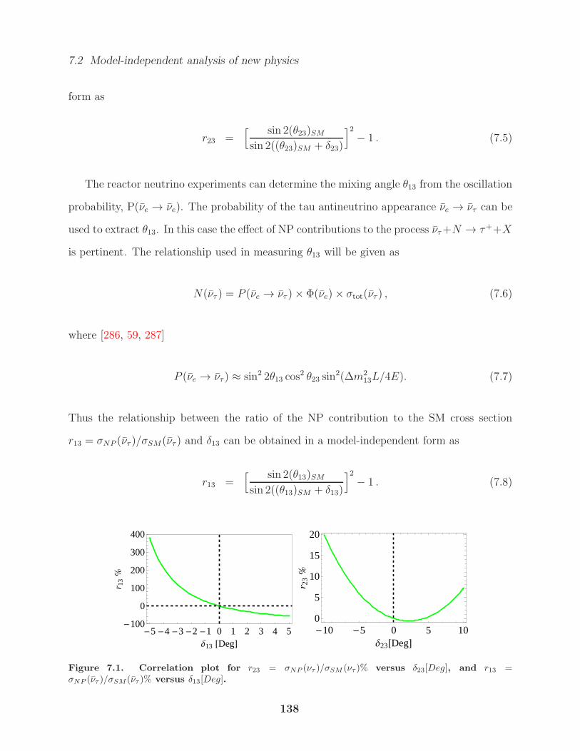
7.2 Model-independent analysis of new physics
form as
r23 =[ sin 2(θ23)SMsin 2((θ23)SM + δ23)
]2− 1 . (7.5)
The reactor neutrino experiments can determine the mixing angle θ13 from the oscillation
probability, P(νe → νe). The probability of the tau antineutrino appearance νe → ντ can be
used to extract θ13. In this case the effect of NP contributions to the process ντ+N → τ++X
is pertinent. The relationship used in measuring θ13 will be given as
N(ντ ) = P (νe → ντ )× Φ(νe)× σtot(ντ ) , (7.6)
where [286, 59, 287]
P (νe → ντ ) ≈ sin2 2θ13 cos2 θ23 sin
2(∆m213L/4E). (7.7)
Thus the relationship between the ratio of the NP contribution to the SM cross section
r13 = σNP (ντ )/σSM(ντ ) and δ13 can be obtained in a model-independent form as
r13 =[ sin 2(θ13)SMsin 2((θ13)SM + δ13)
]2− 1 . (7.8)
-5-4-3-2-1 0 1 2 3 4 5-100
0
100
200
300
400
∆13 @DegD
r 13%
-10 -5 0 5 100
5
10
15
20
∆23@DegD
r 23%
Figure 7.1. Correlation plot for r23 = σNP (ντ )/σSM (ντ )% versus δ23[Deg], and r13 =σNP (ντ )/σSM (ντ )% versus δ13[Deg].
138
7.3 Kinematics and formalism
In Fig. 7.1 we show the correlation between r23(13)% and δ23(13) [Deg]. One can see that
δ23 ∼ −5 requires r23 ∼ 5%. But δ13 ∼ −1 requires r13 ∼ 25%. In the following sections,
we consider specific models of NP to calculate r23 and r13. We will consider a model with a
charged Higgs and a W ′ model with both left- and right-handed couplings.
7.3 Kinematics and formalism
In the interactions ντ (ντ ) + N → τ−(τ+) + X , we define the four-momenta of incoming
neutrino (k), target nucleon (p) and produced τ lepton (k′) in the laboratory frame. The
hadronic invariant mass
W 2 = (p+ q)2, (7.9)
where q = k − k′ is the four-momentum transfer, is defined in the allowed physical region
M ≤W ≤√s−mτ , (7.10)
where s = (k + p)2 is the center of mass energy and M is the average nucleon mass.
The three relevant subprocesses in the neutrino-nucleon interactions are classified accord-
ing to the regions of the hadronic invariant mass W and the momentum transfer q2(= −Q2)
[272]. One can label QE (quasi-elastic scattering) when the hadronic invariant mass is equal
to the nucleon mass W =M , RES (resonance production) when M +mπ < W < Wcut, and
IS (inelastic scattering) when Wcut < W <√s−mτ . Wcut, taken in the region 1.4 GeV∼1.6
GeV, is an empirical boundary between RES and IS processes, to avoid double counting.
The deep inelastic scattering DIS may be labeled within the IS region when Q2 ≥ 1 GeV2,
where the use of the parton model can be justified.
In this work, we consider ∆-resonance state production and neglect all the other higher
139
7.3 Kinematics and formalism
resonance states which give small contributions [288, 289, 290]. One can write
W 2 =M2 + t+ 2p · q, (7.11)
with p · q =M(Ecmν −Ecm
l ) where the energy and momentum of the lepton and the neutrino
in the center of mass (cm) system are
Ecmν =
(s−M2)
2√s
, pcml =√
(Ecml )2 −m2
l ,
Ecml =
(s−M2∆ +m2
l )
2√s
, (7.12)
with (ml, M, M∆) being the masses of the charged lepton, nucleon, and the ∆ state,
respectively. In the lab frame, the charged lepton energy is given by
El =t + 2MEν +M2 −M2
∆
2M. (7.13)
The threshold neutrino energy to create the charged lepton partner in the ∆-RES case is
given by
Ethνl
=(ml +M∆)
2 −M2n
2Mn, (7.14)
which gives Ethνl
= 4.35 GeV in the case of tau neutrino production. Using the allowed range
of the invariant mass in the resonance production, the allowed region of the momentum
transfer t ≡ −Q2 lies in the interval
(M +mπ)2 −
(M2 + 2M(Ecm
ν − Ecml )
)≤ t ≤W 2
cut −(M2 + 2M(Ecm
ν −Ecml )
). (7.15)
In the following three sections, we consider charged Higgs and W ′ effects to the three
processes quasi-elastic interaction, ∆ resonance production and deep inelastic scattering in
the neutrino-nucleon interactions ντ +N → τ− +X and ντ +N → τ+ +X .
140
7.4 Quasielastic neutrino interaction
7.4 Quasielastic neutrino interaction
In this section we will discuss the charged Higgs andW ′ effects to the quasi-elastic interaction.
7.4.1 Quasielastic neutrino interaction − SM
In this section we consider the SM contribution to ντ +n→ τ−+p and ντ +p→ τ++n. We
first summarize the SM results for the quasielastic scattering of a neutrino on a free neutron
target,
νl(k) + n(p) → l−(k′) + p(p′) , (7.16)
where k, k′, p, and p′ denote the four-momenta and l indicates the lepton e, µ, or τ . The
spin-averaged matrix element squared for the above reaction is a convolution of spin-averaged
leptonic and hadronic tensors Lµν and Hµν :
|M|2 = G2F
2LµνHµν . (7.17)
The leptonic tensor calculation is straightforward, but the hadronic tensor involves nonper-
turbative effects. In order to calculate the hadronic tensor, we define the charged hadronic
current for this process:
〈p(p′)|J+µ |n(p)〉 = Vud 〈p(p′)|(Vµ −Aµ)|n(p)〉
= Vud p(p′)Γµn(p). (7.18)
The expressions for the matrix elements of the vector and axial-vector currents are summa-
rized in terms of six form factors in the Appendix D. Due to time reversal invariance, the
form factors are real functions of t = q2. When invariance under charge conjugation holds,
two form factors vanish (FS = 0, FT = 0) [291]. The matrix element, then, can be written
141
7.4 Quasielastic neutrino interaction
as
M =GF cos θc√
2ul(k
′)γµ(1− γ5)uνl(k)
uN ′(p′)
[F V1 (t)γµ + F V
2 (t)iσµνq
ν
2M+ FA(t)γµγ5 + FP (t)γ5
qµM
]uN(p), (7.19)
where N and N ′ are the initial and final nucleons, while l and νl are the final charged lepton
and the initial neutrino. In our case N = n, N ′ = p, l = τ , and νl = ντ .
After evaluating |M|2, one can obtain the SM differential cross section for the reaction
in Eq. (7.16) [291],
dσSM(νl)
dt=
M2G2F cos2 θc
8πE2ν
[ASM +BSM
(s− u)
M2+ CSM
(s− u)2
M4
], (7.20)
where GF = 1.116637 × 10⁻⁵ GeV−2 is the Fermi coupling constant, cos θc = 0.9746 is the
cosine of the Cabibbo angle,MW is theW boson mass, and Eν is the incident neutrino energy.
M = (Mp +Mn)/2 ≈ 938.9 MeV is the nucleon mass, and we neglect the proton-neutron
mass difference. The expressions for the coefficients fSM (f = A,B,C) are summarized in
the Appendix D. The Mandelstam variables are defined by s = (k + p)2, t = q2 = (k − k′)2,
and u = (k − p′)2. The expressions for these variables in terms of Eν and the lepton energy
El are given in the Appendix D.
The quasielastic scattering of an antineutrino on a free nucleon is given by
νl(k) + p(p) → l+(k′) + n(p′) . (7.21)
The charged hadronic current becomes [272, 292]
〈n(p′)|J−µ |p(p)〉 = 〈p(p)|J+
µ |n(p′)〉†
= Vud n(p′)Γµp(p), (7.22)
142
7.4 Quasielastic neutrino interaction
where
Γµ(p, p′) = γ0Γ
†µ(p
′, p)γ0. (7.23)
The relationship between the differential cross sections of ντ+n→ τ−+p and ντ+p→ τ++n
is [292, 293]
dσSM(νl)
dt(s, t, u) =
dσSM(νl)
dt(u, t, s). (7.24)
Thus, the matrix element is given by Eq. 7.19, and the differential cross section, similarly to
Eq. 7.20, is given by
dσSM(νl)
dt=
M2G2F cos2 θc
8πE2ν
[ASM −BSM
(s− u)
M2+ CSM
(s− u)2
M4
]. (7.25)
The negative sign of BSM leads to a relatively smaller cross section for the antineutrino
scattering.
7.4.2 Quasielastic neutrino interaction − Charged Higgs Effect
We consider here the charged Higgs contribution to ντ + n→ τ− + p and ντ + p→ τ+ + n.
Charged Higgs particles appear in multi-Higgs models. In the SM the Higgs couples to the
fermion masses, but in a general multi-Higgs model the charged Higgs may not couple to the
mass. What is true in most models is that the coupling of the charged Higgs to the leptons
is no longer universal. Hence, the extraction of θ23 and θ13 from νµ → νµ and νe → νe
survival probabilities, respectively, will be different from νµ → ντ and νe → ντ probabilities,
respectively, in the presence of a charged Higgs effect.
The most general coupling of the charged Higgs is
L =g
2√2
[Vuidj ui(g
uidjS ± g
uidjP γ5)dj + νi(g
νiljS ± g
νiljP γ5)lj
]H±, (7.26)
143
7.4 Quasielastic neutrino interaction
where ui and dj refer to up and down type quarks, and νi and lj refer to neutrinos and charged
leptons. The other parameters are as follows: g = e/ sin θW is the SM weak coupling constant,
Vuidj is the CKM matrix element, and gS,P are the scalar and pseudoscalar couplings of the
charged Higgs to fermions. Here, in this work, we assume the couplings gS,P are real.
We will choose the couplings gS,P , relevant for ντ +n→ τ−+p and ντ +p→ τ++n, to be
given by the two Higgs doublet model of type II (2HDM II). In the 2HDM II these couplings
are related to couplings in other sectors and so can be constrained by measurements in these
other sectors. However, in our analysis, to keep things general we will not assume any relation
between the couplings gS,P and the couplings in other sectors, thereby avoiding constraints
from other sectors. To constrain the couplings gS,P we will only consider processes that are
generated by ONP = uΓidτΓjντ . In the 2HDM II, constrains on the model parameters come
from various sectors [294]. These constraints turn out to be similar but slightly stronger
than the ones obtained in our analysis.
The coupling of charged Higgs boson (H±) interactions to a SM fermion in the 2HDM II
is [295]
L =g√2MW
∑
ij
[mui
cotβ uiVijPL,Rdj +mdj tanβ uiVijPR,Ldj +mlj tanβ νiPR,Llj
]H±,
(7.27)
where PL,R = (1∓ γ5)/2, and tanβ is the ratio between the two vacuum expectation values
(vev’s) of the two Higgs doublets. Comparing Eq. (7.45) and Eq. (7.27), one can obtain
guidjS =
(mdj tan β +mui
cot β
MW
),
guidjP =
(mdj tan β −mui
cot β
MW
),
gνiljS = g
νiljP =
mlj tanβ
MW. (7.28)
Constraints on the size of the operator ONP = uΓidτΓjντ can be obtained from the
144
7.4 Quasielastic neutrino interaction
branching ratio of the decay τ− → π−ντ . In the presence of a charged Higgs, the branching
ratio for this process is
BrSM+Hτ−→π−ντ
= BrSMτ−→π−ντ(1 + rπ
2
H ) , (7.29)
where the charged Higgs contribution is
rπH =(mu −md tan
2 β
mu +md
)m2π
m2H
. (7.30)
The SM branching ratio is related to the tau lepton width (Γτ ) and the decay rate(ΓSMτ−→π−ντ
)
as BrSMτ−→π−ντ= ΓSM
τ−→π−ντ/Γτ with
ΓSMτ−→π−ντ
=G2
F
16π|Vud|2f 2
πm3τ
(1− m2
π
m2τ
)2
δτ/π . (7.31)
Here δτ/π = 1.0016 ± 0.0014 [296] is the radiative correction. Further, the SM branching
ratio can also be expressed as [297]
BrSMτ−→π−ντ = 0.607Br(τ− → ντe−νe) = 10.82± 0.02% , (7.32)
while the measured Br(τ− → π−ντ )exp = (10.91 ± 0.07)% [168]. In Fig. 7.2 we show the
constraints on mH − tanβ from τ− → π−ντ . From Eq. 7.27 we can construct the NSI
parameters defined in Ref [280] as εud(L)ττ ≡ mumτ
m2H
and εud(R)ττ ≡ mdmτ tan2 β
m2H
. We find that the
constraints on the effective operator considered in this work are consistent with the one in
Ref. [280]. Finally, we note that τ has a significant branching ratio to τ− → ρ−ντ [168].
However, a charged Higgs cannot contribute to this decay, and hence there is no constraint
on the charged Higgs couplings from this decay [282].
Keeping in mind the constraints from Fig. (7.2), we calculate the charged Higgs contribu-
tion to ντ +n→ τ−+p. The modified differential cross section for the reaction in Eq. (7.16)
145
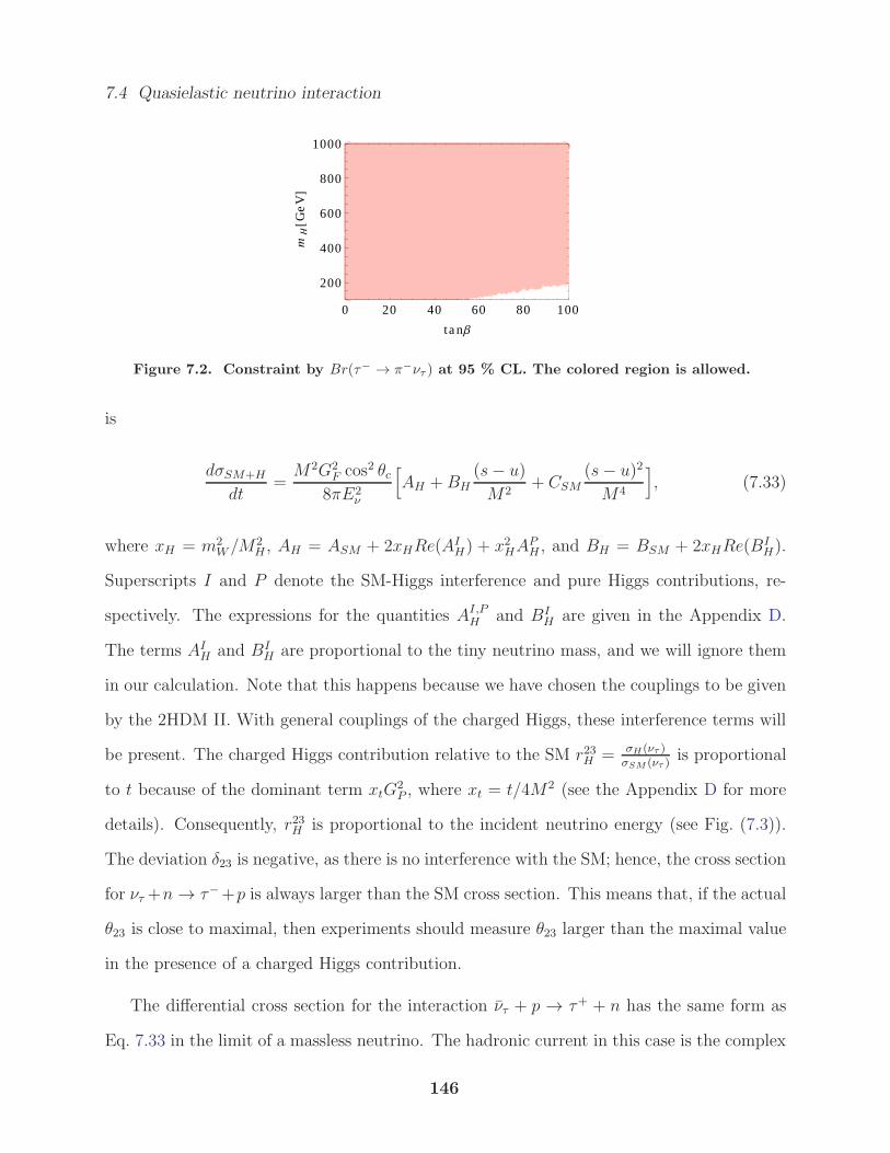
7.4 Quasielastic neutrino interaction
0 20 40 60 80 100
200
400
600
800
1000
ta nΒ
mH@G
eVD
Figure 7.2. Constraint by Br(τ− → π−ντ ) at 95 % CL. The colored region is allowed.
is
dσSM+H
dt=M2G2
F cos2 θc8πE2
ν
[AH +BH
(s− u)
M2+ CSM
(s− u)2
M4
], (7.33)
where xH = m2W/M
2H , AH = ASM + 2xHRe(A
IH) + x2HA
PH , and BH = BSM + 2xHRe(B
IH).
Superscripts I and P denote the SM-Higgs interference and pure Higgs contributions, re-
spectively. The expressions for the quantities AI,PH and BI
H are given in the Appendix D.
The terms AIH and BI
H are proportional to the tiny neutrino mass, and we will ignore them
in our calculation. Note that this happens because we have chosen the couplings to be given
by the 2HDM II. With general couplings of the charged Higgs, these interference terms will
be present. The charged Higgs contribution relative to the SM r23H = σH (ντ )σSM (ντ )
is proportional
to t because of the dominant term xtG2P , where xt = t/4M2 (see the Appendix D for more
details). Consequently, r23H is proportional to the incident neutrino energy (see Fig. (7.3)).
The deviation δ23 is negative, as there is no interference with the SM; hence, the cross section
for ντ +n→ τ−+p is always larger than the SM cross section. This means that, if the actual
θ23 is close to maximal, then experiments should measure θ23 larger than the maximal value
in the presence of a charged Higgs contribution.
The differential cross section for the interaction ντ + p → τ+ + n has the same form as
Eq. 7.33 in the limit of a massless neutrino. The hadronic current in this case is the complex
146
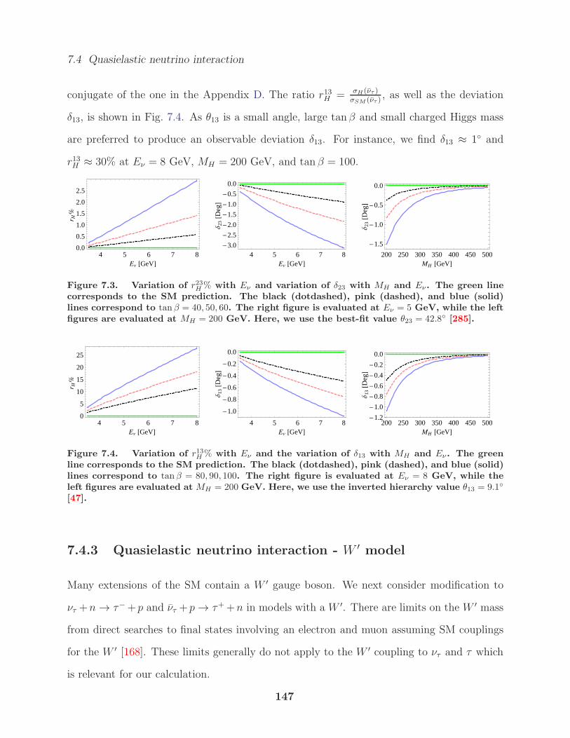
7.4 Quasielastic neutrino interaction
conjugate of the one in the Appendix D. The ratio r13H = σH (ντ )σSM (ντ )
, as well as the deviation
δ13, is shown in Fig. 7.4. As θ13 is a small angle, large tan β and small charged Higgs mass
are preferred to produce an observable deviation δ13. For instance, we find δ13 ≈ 1 and
r13H ≈ 30% at Eν = 8 GeV, MH = 200 GeV, and tan β = 100.
4 5 6 7 80.0
0.5
1.0
1.5
2.0
2.5
EΝ @GeVD
r H%
4 5 6 7 8-3.0
-2.5
-2.0
-1.5
-1.0
-0.5
0.0
EΝ @GeVD
∆23@D
egD
200 250 300 350 400 450 500
-1.5
-1.0
-0.5
0.0
MH @GeVD
∆23@D
egD
Figure 7.3. Variation of r23H% with Eν and variation of δ23 with MH and Eν. The green line
corresponds to the SM prediction. The black (dotdashed), pink (dashed), and blue (solid)lines correspond to tanβ = 40, 50, 60. The right figure is evaluated at Eν = 5 GeV, while the leftfigures are evaluated at MH = 200 GeV. Here, we use the best-fit value θ23 = 42.8 [285].
4 5 6 7 80
5
10
15
20
25
EΝ @GeVD
r H%
4 5 6 7 8
-1.0
-0.8
-0.6
-0.4
-0.2
0.0
EΝ @GeVD
∆13@D
egD
200 250 300 350 400 450 500-1.2
-1.0
-0.8
-0.6
-0.4
-0.2
0.0
MH @GeVD
∆13@D
egD
Figure 7.4. Variation of r13H% with Eν and the variation of δ13 with MH and Eν . The green
line corresponds to the SM prediction. The black (dotdashed), pink (dashed), and blue (solid)lines correspond to tanβ = 80, 90, 100. The right figure is evaluated at Eν = 8 GeV, while theleft figures are evaluated at MH = 200 GeV. Here, we use the inverted hierarchy value θ13 = 9.1
[47].
7.4.3 Quasielastic neutrino interaction - W ′ model
Many extensions of the SM contain a W ′ gauge boson. We next consider modification to
ντ +n→ τ−+ p and ντ + p→ τ++n in models with a W ′. There are limits on the W ′ mass
from direct searches to final states involving an electron and muon assuming SM couplings
for the W ′ [168]. These limits generally do not apply to the W ′ coupling to ντ and τ which
is relevant for our calculation.
147
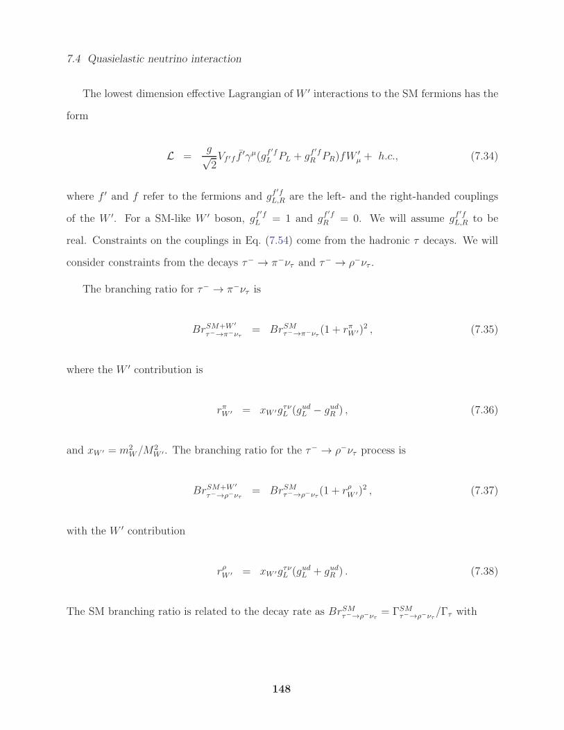
7.4 Quasielastic neutrino interaction
The lowest dimension effective Lagrangian of W ′ interactions to the SM fermions has the
form
L =g√2Vf ′f f
′γµ(gf′f
L PL + gf′f
R PR)fW′µ + h.c., (7.34)
where f ′ and f refer to the fermions and gf′f
L,R are the left- and the right-handed couplings
of the W ′. For a SM-like W ′ boson, gf′f
L = 1 and gf′f
R = 0. We will assume gf′f
L,R to be
real. Constraints on the couplings in Eq. (7.54) come from the hadronic τ decays. We will
consider constraints from the decays τ− → π−ντ and τ− → ρ−ντ .
The branching ratio for τ− → π−ντ is
BrSM+W ′
τ−→π−ντ= BrSMτ−→π−ντ
(1 + rπW ′)2 , (7.35)
where the W ′ contribution is
rπW ′ = xW ′gτνL (gudL − gudR ) , (7.36)
and xW ′ = m2W/M
2W ′. The branching ratio for the τ− → ρ−ντ process is
BrSM+W ′
τ−→ρ−ντ= BrSMτ−→ρ−ντ
(1 + rρW ′)2 , (7.37)
with the W ′ contribution
rρW ′ = xW ′gτνL (gudL + gudR ) . (7.38)
The SM branching ratio is related to the decay rate as BrSMτ−→ρ−ντ= ΓSM
τ−→ρ−ντ/Γτ with
148
7.4 Quasielastic neutrino interaction
ΓSMτ−→ρ−ντ
=G2
F
16π|Vud|2f 2
ρm3τ
(1−
m2ρ
m2τ
)2(1 +
2m2ρ
m2τ
), (7.39)
where fρ = 223 MeV [298]. Further, the SM branching ratio can also be expressed as [297]
BrSMτ−→ρ−ντ= 1.23Br(τ− → ντe
−νe) = 21.92± 0.05% . (7.40)
The measured branching ratio is Br(τ− → ρ−ντ )exp = (23.1± 0.98)% [168].
Figures 7.5 and 7.6 show the allowed regions for the W ′ couplings. The couplings are
uniformly varied in the range [−2, 2] and constrained by the measured τ− → π−ντ and
τ− → ρ−ντ branching ratios with 1σ errors. From Eqs. (7.36, 7.38), the case with a pure
left-handed W ′ coupling is allowed, as shown in Figs. (7.5, 7.6). The constraints on the
effective operator are consistent with the one in Ref. [280]. From Eq. 7.54 the NSI parameter
εud(L,R)ττ defined in Ref. [280] is given as ε
ud(L,R)ττ ≡ gτνL g
ud(L,R)(
MW
MW ′)2.
-2.0-1.5-1.0-0.5 0.0 0.5 1.0 1.5 2.0-2.0
-1.5
-1.0
-0.5
0.0
0.5
1.0
1.5
2.0
g Lu d
gLΤΝ
Figure 7.5. The constraints on the W ′ couplings without right-handed coupling at MW ′ =500 − 1000 GeV. The constraints are from τ− → π−ντ and τ− → ρ−ντ branching ratios. Theerrors in the branching ratios are varied within 1σ. The colored regions are allowed.
In the presence of the W ′ gauge boson, we can obtain the modified differential cross
149
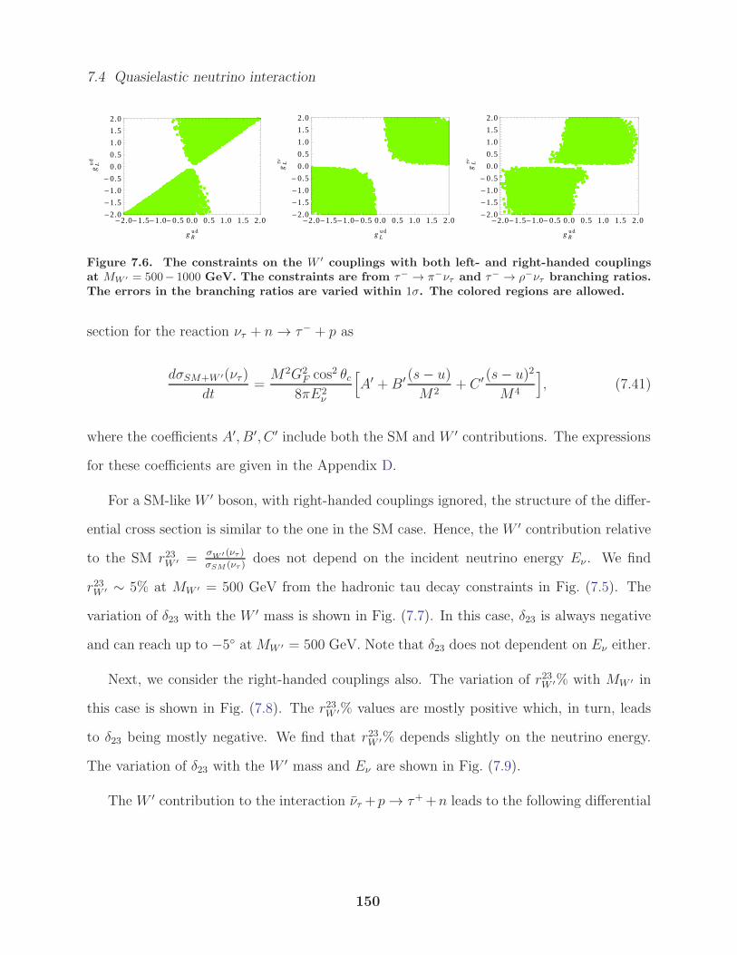
7.4 Quasielastic neutrino interaction
-2.0-1.5-1.0-0.5 0.0 0.5 1.0 1.5 2.0-2.0
-1.5
-1.0
-0.5
0.0
0.5
1.0
1.5
2.0
g Ru d
gLu
d
-2.0-1.5-1.0-0.5 0.0 0.5 1.0 1.5 2.0-2.0
-1.5
-1.0
-0.5
0.0
0.5
1.0
1.5
2.0
g Lu d
gLΤΝ
-2.0-1.5-1.0-0.5 0.0 0.5 1.0 1.5 2.0-2.0
-1.5
-1.0
-0.5
0.0
0.5
1.0
1.5
2.0
g Ru d
gLΤΝ
Figure 7.6. The constraints on the W ′ couplings with both left- and right-handed couplingsat MW ′ = 500− 1000 GeV. The constraints are from τ− → π−ντ and τ− → ρ−ντ branching ratios.The errors in the branching ratios are varied within 1σ. The colored regions are allowed.
section for the reaction ντ + n→ τ− + p as
dσSM+W ′(ντ )
dt=M2G2
F cos2 θc8πE2
ν
[A′ +B′ (s− u)
M2+ C ′ (s− u)2
M4
], (7.41)
where the coefficients A′, B′, C ′ include both the SM and W ′ contributions. The expressions
for these coefficients are given in the Appendix D.
For a SM-like W ′ boson, with right-handed couplings ignored, the structure of the differ-
ential cross section is similar to the one in the SM case. Hence, the W ′ contribution relative
to the SM r23W ′ =σW ′ (ντ )
σSM (ντ )does not depend on the incident neutrino energy Eν . We find
r23W ′ ∼ 5% at MW ′ = 500 GeV from the hadronic tau decay constraints in Fig. (7.5). The
variation of δ23 with the W ′ mass is shown in Fig. (7.7). In this case, δ23 is always negative
and can reach up to −5 atMW ′ = 500 GeV. Note that δ23 does not dependent on Eν either.
Next, we consider the right-handed couplings also. The variation of r23W ′% with MW ′ in
this case is shown in Fig. (7.8). The r23W ′% values are mostly positive which, in turn, leads
to δ23 being mostly negative. We find that r23W ′% depends slightly on the neutrino energy.
The variation of δ23 with the W ′ mass and Eν are shown in Fig. (7.9).
The W ′ contribution to the interaction ντ +p→ τ++n leads to the following differential
150
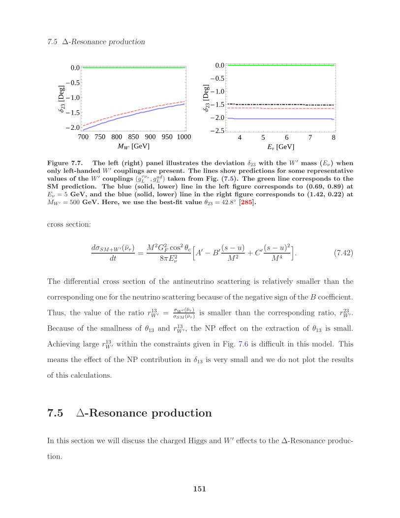
7.5 ∆-Resonance production
700 750 800 850 900 950 1000-2.0
-1.5
-1.0
-0.5
0.0
MW ' @GeVD
∆23@D
egD
4 5 6 7 8-2.5
-2.0
-1.5
-1.0
-0.5
0.0
EΝ @GeVD
∆23@D
egD
Figure 7.7. The left (right) panel illustrates the deviation δ23 with the W ′ mass (Eν) whenonly left-handed W ′ couplings are present. The lines show predictions for some representativevalues of the W ′ couplings (gτντ
L, gud
L) taken from Fig. (7.5). The green line corresponds to the
SM prediction. The blue (solid, lower) line in the left figure corresponds to (0.69, 0.89) atEν = 5 GeV, and the blue (solid, lower) line in the right figure corresponds to (1.42, 0.22) atMW ′ = 500 GeV. Here, we use the best-fit value θ23 = 42.8 [285].
cross section:
dσSM+W ′(ντ )
dt=M2G2
F cos2 θc8πE2
ν
[A′ − B′ (s− u)
M2+ C ′ (s− u)2
M4
]. (7.42)
The differential cross section of the antineutrino scattering is relatively smaller than the
corresponding one for the neutrino scattering because of the negative sign of the B coefficient.
Thus, the value of the ratio r13W ′ =σW ′ (ντ )
σSM (ντ )is smaller than the corresponding ratio, r23W ′.
Because of the smallness of θ13 and r13W ′, the NP effect on the extraction of θ13 is small.
Achieving large r13W ′ within the constraints given in Fig. 7.6 is difficult in this model. This
means the effect of the NP contribution in δ13 is very small and we do not plot the results
of this calculations.
7.5 ∆-Resonance production
In this section we will discuss the charged Higgs and W ′ effects to the ∆-Resonance produc-
tion.
151
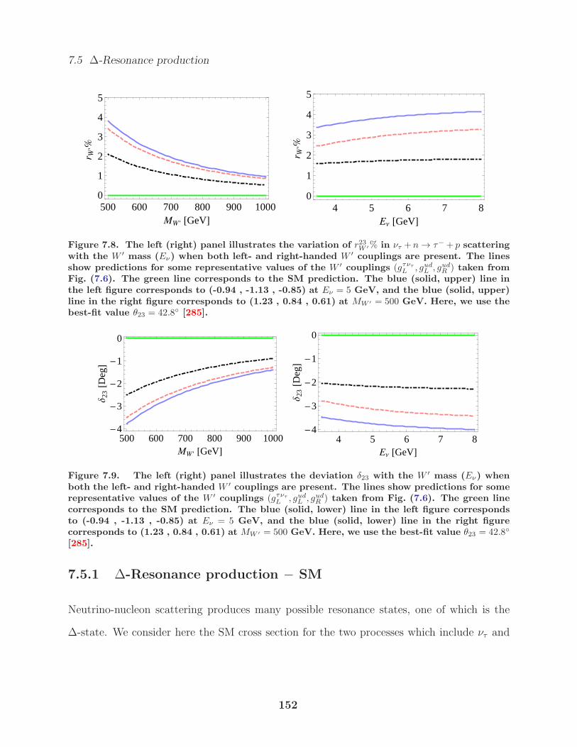
7.5 ∆-Resonance production
500 600 700 800 900 10000
1
2
3
4
5
MW ' @GeVD
r W'%
4 5 6 7 80
1
2
3
4
5
EΝ @GeVD
r W'%
Figure 7.8. The left (right) panel illustrates the variation of r23W ′% in ντ +n → τ− + p scattering
with the W ′ mass (Eν) when both left- and right-handed W ′ couplings are present. The linesshow predictions for some representative values of the W ′ couplings (gτντ
L, gud
L, gud
R) taken from
Fig. (7.6). The green line corresponds to the SM prediction. The blue (solid, upper) line inthe left figure corresponds to (-0.94 , -1.13 , -0.85) at Eν = 5 GeV, and the blue (solid, upper)line in the right figure corresponds to (1.23 , 0.84 , 0.61) at MW ′ = 500 GeV. Here, we use thebest-fit value θ23 = 42.8 [285].
500 600 700 800 900 1000-4
-3
-2
-1
0
MW ' @GeVD
∆23@D
egD
4 5 6 7 8-4
-3
-2
-1
0
EΝ @GeVD
∆23@D
egD
Figure 7.9. The left (right) panel illustrates the deviation δ23 with the W ′ mass (Eν) whenboth the left- and right-handed W ′ couplings are present. The lines show predictions for somerepresentative values of the W ′ couplings (gτντ
L, gud
L, gud
R) taken from Fig. (7.6). The green line
corresponds to the SM prediction. The blue (solid, lower) line in the left figure correspondsto (-0.94 , -1.13 , -0.85) at Eν = 5 GeV, and the blue (solid, lower) line in the right figurecorresponds to (1.23 , 0.84 , 0.61) at MW ′ = 500 GeV. Here, we use the best-fit value θ23 = 42.8
[285].
7.5.1 ∆-Resonance production − SM
Neutrino-nucleon scattering produces many possible resonance states, one of which is the
∆-state. We consider here the SM cross section for the two processes which include ντ and
152
7.5 ∆-Resonance production
ντ ,
ντ + n→ τ− +∆+,
ντ + p→ τ+ +∆0. (7.43)
from the Hagiwara model [272]. That will represent the starting point of our original compu-
tation of NP effects due to charged Higgs andW ′. Details of the SM cross section calculations
can be found in Ref. [272]. The hadronic tensor is written as
WRESµν =
cos2 θc4
Tr[P βαΓµα(p/+M)Γνβ
] 1π
WΓ(W )
(W 2 −M2∆)
2 +W 2Γ2(W ). (7.44)
Within the kinematical region of M +mπ < W < Wcut with Wcut = 1.4 GeV, we estimate
the total cross section of the ∆ production (∆-RES) process by integrating over Eτ and
cos θ.
7.5.2 ∆-Resonance production − Charged Higgs Effect
We consider here the charged Higgs contribution to ντ +n→ τ−+∆+ and ντ +p→ τ++∆0.
As considered in the previous section, we choose the couplings of charged Higgs interactions
to the SM fermions to be given by the two Higgs doublet model of type II (2HDM II) [295]
L =g
2√2
[Vuidj ui(g
uidjS ± g
uidjP γ5)dj + νi(g
νiljS ± g
νiljP γ5)lj
]H±, (7.45)
where ui and dj refer to up and down type quarks, and νi and lj refer to neutrinos and the
corresponding charged leptons. The other parameters are as follows: g = e/ sin θW is the
SM weak coupling constant, Vuidj is the CKM matrix element, and gS,P are the scalar and
pseudoscalar couplings of the charged Higgs to fermions. Here, in this work, we assume the
153
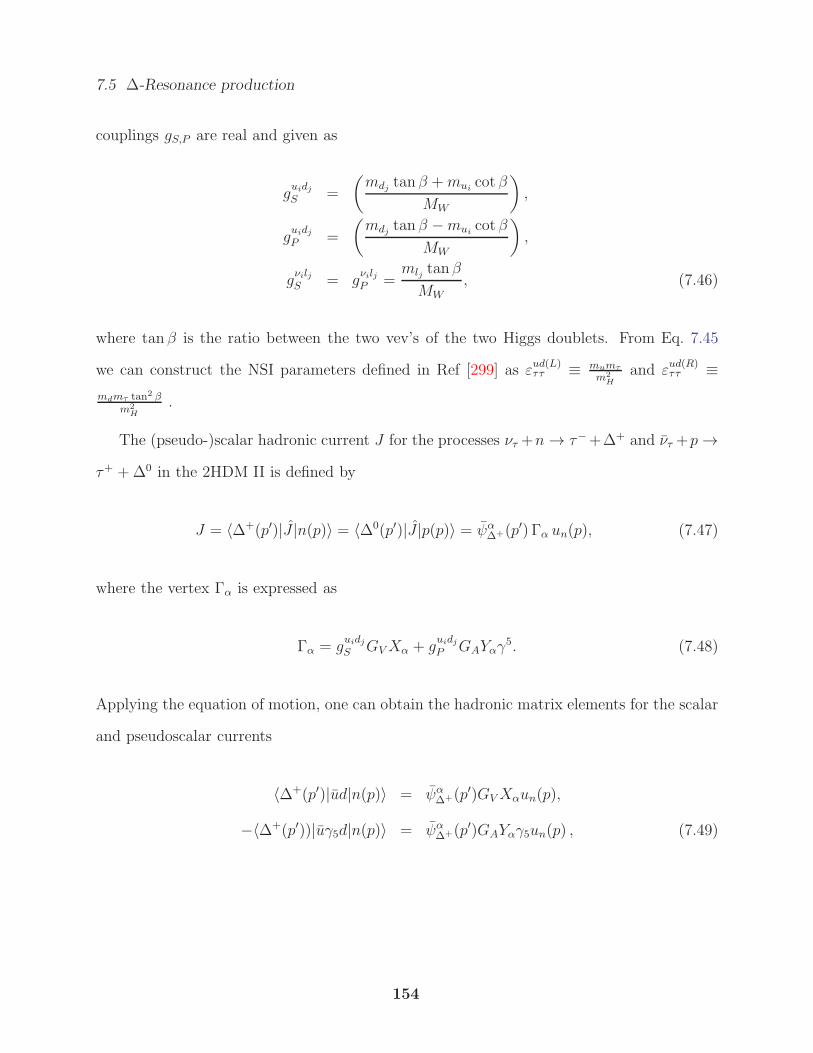
7.5 ∆-Resonance production
couplings gS,P are real and given as
guidjS =
(mdj tan β +mui
cot β
MW
),
guidjP =
(mdj tan β −mui
cot β
MW
),
gνiljS = g
νiljP =
mlj tanβ
MW, (7.46)
where tan β is the ratio between the two vev’s of the two Higgs doublets. From Eq. 7.45
we can construct the NSI parameters defined in Ref [299] as εud(L)ττ ≡ mumτ
m2H
and εud(R)ττ ≡
mdmτ tan2 βm2
H.
The (pseudo-)scalar hadronic current J for the processes ντ +n→ τ−+∆+ and ντ +p→
τ+ +∆0 in the 2HDM II is defined by
J = 〈∆+(p′)|J |n(p)〉 = 〈∆0(p′)|J|p(p)〉 = ψα∆+(p′) Γα un(p), (7.47)
where the vertex Γα is expressed as
Γα = guidjS GVXα + g
uidjP GAYαγ
5. (7.48)
Applying the equation of motion, one can obtain the hadronic matrix elements for the scalar
and pseudoscalar currents
〈∆+(p′)|ud|n(p)〉 = ψα∆+(p′)GVXαun(p),
−〈∆+(p′))|uγ5d|n(p)〉 = ψα∆+(p′)GAYαγ5un(p) , (7.49)
154
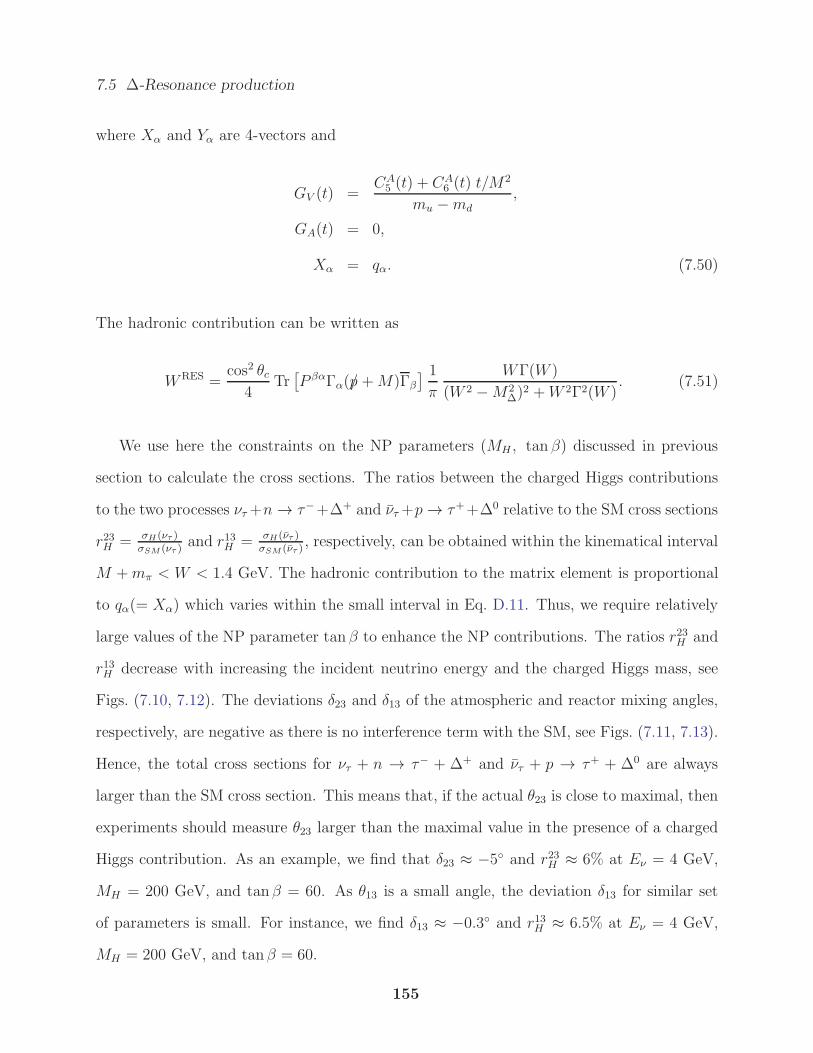
7.5 ∆-Resonance production
where Xα and Yα are 4-vectors and
GV (t) =CA
5 (t) + CA6 (t) t/M
2
mu −md,
GA(t) = 0,
Xα = qα. (7.50)
The hadronic contribution can be written as
WRES =cos2 θc
4Tr
[P βαΓα(p/ +M)Γβ
] 1π
WΓ(W )
(W 2 −M2∆)
2 +W 2Γ2(W ). (7.51)
We use here the constraints on the NP parameters (MH , tan β) discussed in previous
section to calculate the cross sections. The ratios between the charged Higgs contributions
to the two processes ντ+n→ τ−+∆+ and ντ+p→ τ++∆0 relative to the SM cross sections
r23H = σH (ντ )σSM (ντ )
and r13H = σH (ντ )σSM (ντ )
, respectively, can be obtained within the kinematical interval
M +mπ < W < 1.4 GeV. The hadronic contribution to the matrix element is proportional
to qα(= Xα) which varies within the small interval in Eq. D.11. Thus, we require relatively
large values of the NP parameter tan β to enhance the NP contributions. The ratios r23H and
r13H decrease with increasing the incident neutrino energy and the charged Higgs mass, see
Figs. (7.10, 7.12). The deviations δ23 and δ13 of the atmospheric and reactor mixing angles,
respectively, are negative as there is no interference term with the SM, see Figs. (7.11, 7.13).
Hence, the total cross sections for ντ + n → τ− + ∆+ and ντ + p → τ+ + ∆0 are always
larger than the SM cross section. This means that, if the actual θ23 is close to maximal, then
experiments should measure θ23 larger than the maximal value in the presence of a charged
Higgs contribution. As an example, we find that δ23 ≈ −5 and r23H ≈ 6% at Eν = 4 GeV,
MH = 200 GeV, and tanβ = 60. As θ13 is a small angle, the deviation δ13 for similar set
of parameters is small. For instance, we find δ13 ≈ −0.3 and r13H ≈ 6.5% at Eν = 4 GeV,
MH = 200 GeV, and tanβ = 60.
155
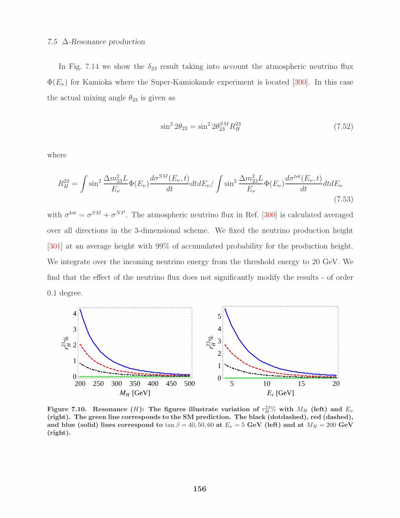
7.5 ∆-Resonance production
In Fig. 7.14 we show the δ23 result taking into account the atmospheric neutrino flux
Φ(Eν) for Kamioka where the Super-Kamiokande experiment is located [300]. In this case
the actual mixing angle θ23 is given as
sin2 2θ23 = sin2 2θSM23 R23H (7.52)
where
R23H =
∫sin2 ∆m
223L
EνΦ(Eν)
dσSM(Eν , t)
dtdtdEν/
∫sin2 ∆m
223L
EνΦ(Eν)
dσtot(Eν , t)
dtdtdEν
(7.53)
with σtot = σSM + σNP . The atmospheric neutrino flux in Ref. [300] is calculated averaged
over all directions in the 3-dimensional scheme. We fixed the neutrino production height
[301] at an average height with 99% of accumulated probability for the production height.
We integrate over the incoming neutrino energy from the threshold energy to 20 GeV. We
find that the effect of the neutrino flux does not significantly modify the results - of order
0.1 degree.
200 250 300 350 400 450 5000
1
2
3
4
MH @GeVD
r H23%
5 10 15 200
1
2
3
4
5
EΝ @GeVD
r H23%
Figure 7.10. Resonance (H): The figures illustrate variation of r23H% with MH (left) and Eν
(right). The green line corresponds to the SM prediction. The black (dotdashed), red (dashed),and blue (solid) lines correspond to tanβ = 40, 50, 60 at Eν = 5 GeV (left) and at MH = 200 GeV(right).
156
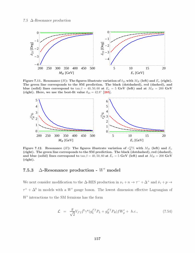
7.5 ∆-Resonance production
200 250 300 350 400 450 500-4
-3
-2
-1
0
MH @GeVD
∆23@D
egD
5 10 15 20
-4
-3
-2
-1
0
EΝ @GeVD
∆23@D
egD
Figure 7.11. Resonance (H): The figures illustrate variation of δ23 with MH (left) and Eν (right).The green line corresponds to the SM prediction. The black (dotdashed), red (dashed), andblue (solid) lines correspond to tanβ = 40, 50, 60 at Eν = 5 GeV (left) and at MH = 200 GeV(right). Here, we use the best-fit value θ23 = 42.8 [285].
200 250 300 350 400 450 5000
1
2
3
4
5
MH @GeVD
r H13%
5 10 15 200
1
2
3
4
5
6
EΝ @GeVD
r H13%
Figure 7.12. Resonance (H): The figures illustrate variation of r13H% with MH (left) and Eν
(right). The green line corresponds to the SM prediction. The black (dotdashed), red (dashed),and blue (solid) lines correspond to tanβ = 40, 50, 60 at Eν = 5 GeV (left) and at MH = 200 GeV(right).
7.5.3 ∆-Resonance production - W ′ model
We next consider modification to the ∆-RES production in ντ +n→ τ− +∆+ and ντ + p→
τ+ + ∆0 in models with a W ′ gauge boson. The lowest dimension effective Lagrangian of
W ′ interactions to the SM fermions has the form
L =g√2Vf ′f f
′γµ(gf′f
L PL + gf′f
R PR)fW′µ + h.c., (7.54)
157
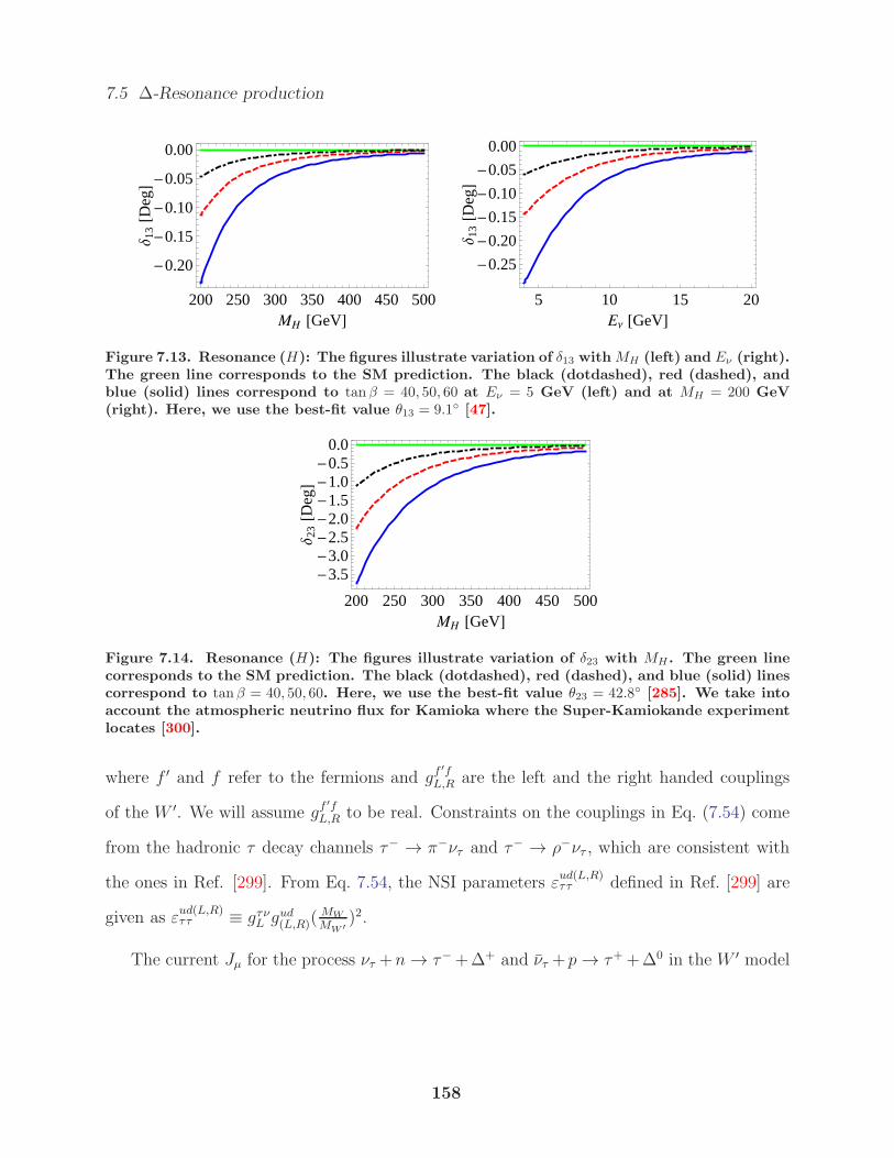
7.5 ∆-Resonance production
200 250 300 350 400 450 500
-0.20
-0.15
-0.10
-0.05
0.00
MH @GeVD
∆13@D
egD
5 10 15 20
-0.25
-0.20
-0.15
-0.10
-0.05
0.00
EΝ @GeVD
∆13@D
egD
Figure 7.13. Resonance (H): The figures illustrate variation of δ13 with MH (left) and Eν (right).The green line corresponds to the SM prediction. The black (dotdashed), red (dashed), andblue (solid) lines correspond to tanβ = 40, 50, 60 at Eν = 5 GeV (left) and at MH = 200 GeV(right). Here, we use the best-fit value θ13 = 9.1 [47].
200 250 300 350 400 450 500
-3.5-3.0-2.5-2.0-1.5-1.0-0.5
0.0
MH @GeVD
∆23@D
egD
Figure 7.14. Resonance (H): The figures illustrate variation of δ23 with MH . The green linecorresponds to the SM prediction. The black (dotdashed), red (dashed), and blue (solid) linescorrespond to tanβ = 40, 50, 60. Here, we use the best-fit value θ23 = 42.8 [285]. We take intoaccount the atmospheric neutrino flux for Kamioka where the Super-Kamiokande experimentlocates [300].
where f ′ and f refer to the fermions and gf′f
L,R are the left and the right handed couplings
of the W ′. We will assume gf′f
L,R to be real. Constraints on the couplings in Eq. (7.54) come
from the hadronic τ decay channels τ− → π−ντ and τ− → ρ−ντ , which are consistent with
the ones in Ref. [299]. From Eq. 7.54, the NSI parameters εud(L,R)ττ defined in Ref. [299] are
given as εud(L,R)ττ ≡ gτνL g
ud(L,R)(
MW
MW ′)2.
The current Jµ for the process ντ +n→ τ−+∆+ and ντ + p→ τ++∆0 in the W ′ model
158
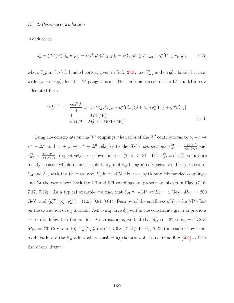
7.5 ∆-Resonance production
is defined as
Jµ = 〈∆+(p′)|Jµ|n(p)〉 = 〈∆0(p′)|Jµ|p(p)〉 = ψα∆+(p′) (gudL Γµα + gudR Γ′
µα) un(p), (7.55)
where Γµα is the left-handed vertex, given in Ref. [272], and Γ′µα is the right-handed vertex,
with (γ5 → −γ5), for the W ′ gauge boson. The hadronic tensor in the W ′ model is now
calculated from
WRESµν =
cos2 θc4
Tr[P βα(gudL Γµα + gudR Γ′
µα)(p/+M)(gudL Γνβ + gudR Γ′νβ)
]
1
π
WΓ(W )
(W 2 −M2∆)
2 +W 2Γ2(W ). (7.56)
Using the constraints on the W ′ couplings, the ratios of the W ′ contributions to ντ +n→
τ− + ∆+ and ντ + p → τ+ + ∆0 relative to the SM cross sections r23W ′ =σW ′ (ντ )
σSM (ντ )and
r13W ′ =σW ′ (ντ )
σSM (ντ ), respectively, are shown in Figs. (7.15, 7.18). The r23W ′ and r13W ′ values are
mostly positive which, in turn, leads to δ23 and δ13 being mostly negative. The variation of
δ23 and δ13 with the W ′ mass and Eν in the SM-like case, with only left-handed couplings,
and for the case where both the LH and RH couplings are present are shown in Figs. (7.16,
7.17, 7.19). As a typical example, we find that δ23 ≈ −14 at Eν = 4 GeV, MW ′ = 200
GeV, and (gτντL , gudL , gudR ) = (1.23, 0.84, 0.61). Because of the smallness of θ13, the NP effect
on the extraction of θ13 is small. Achieving large δ13 within the constraints given in previous
section is difficult in this model. As an example, we find that δ13 ≈ −2 at Eν = 4 GeV,
MW ′ = 200 GeV, and (gτντL , gudL , gudR ) = (1.23, 0.84, 0.61). In Fig. 7.20, the results show small
modification to the δ23 values when considering the atmospheric neutrino flux [300] - of the
size of one degree.
159
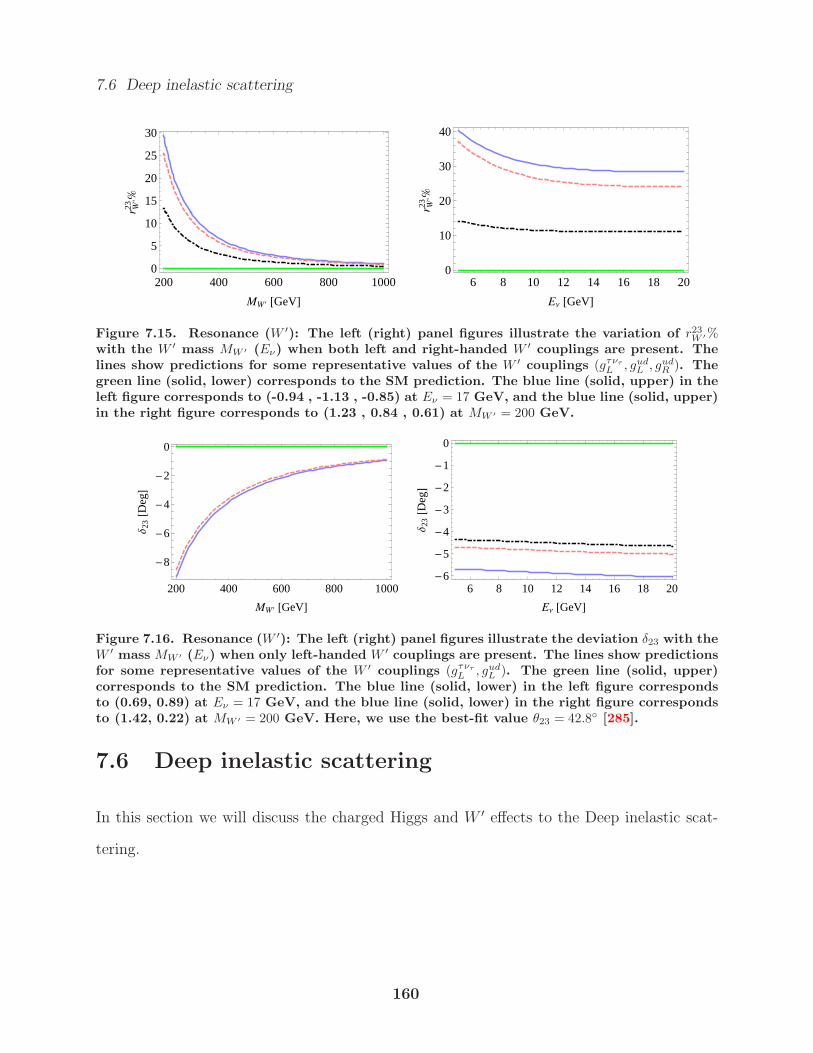
7.6 Deep inelastic scattering
200 400 600 800 10000
5
10
15
20
25
30
MW ' @GeVD
r W'
23%
6 8 10 12 14 16 18 200
10
20
30
40
EΝ @GeVD
r W'
23%
Figure 7.15. Resonance (W ′): The left (right) panel figures illustrate the variation of r23W ′%
with the W ′ mass MW ′ (Eν) when both left and right-handed W ′ couplings are present. Thelines show predictions for some representative values of the W ′ couplings (gτντ
L, gud
L, gud
R). The
green line (solid, lower) corresponds to the SM prediction. The blue line (solid, upper) in theleft figure corresponds to (-0.94 , -1.13 , -0.85) at Eν = 17 GeV, and the blue line (solid, upper)in the right figure corresponds to (1.23 , 0.84 , 0.61) at MW ′ = 200 GeV.
200 400 600 800 1000
-8
-6
-4
-2
0
MW ' @GeVD
∆23@D
egD
6 8 10 12 14 16 18 20-6
-5
-4
-3
-2
-1
0
EΝ @GeVD
∆23@D
egD
Figure 7.16. Resonance (W ′): The left (right) panel figures illustrate the deviation δ23 with theW ′ mass MW ′ (Eν) when only left-handed W ′ couplings are present. The lines show predictionsfor some representative values of the W ′ couplings (gτντ
L, gud
L). The green line (solid, upper)
corresponds to the SM prediction. The blue line (solid, lower) in the left figure correspondsto (0.69, 0.89) at Eν = 17 GeV, and the blue line (solid, lower) in the right figure correspondsto (1.42, 0.22) at MW ′ = 200 GeV. Here, we use the best-fit value θ23 = 42.8 [285].
7.6 Deep inelastic scattering
In this section we will discuss the charged Higgs and W ′ effects to the Deep inelastic scat-
tering.
160
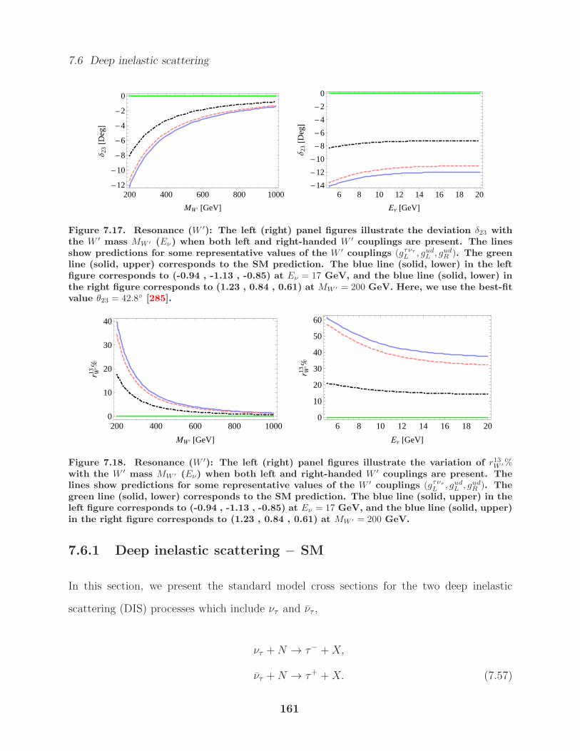
7.6 Deep inelastic scattering
200 400 600 800 1000-12
-10
-8
-6
-4
-2
0
MW ' @GeVD
∆23@D
egD
6 8 10 12 14 16 18 20-14
-12
-10
-8
-6
-4
-2
0
EΝ @GeVD
∆23@D
egD
Figure 7.17. Resonance (W ′): The left (right) panel figures illustrate the deviation δ23 withthe W ′ mass MW ′ (Eν) when both left and right-handed W ′ couplings are present. The linesshow predictions for some representative values of the W ′ couplings (gτντ
L, gud
L, gud
R). The green
line (solid, upper) corresponds to the SM prediction. The blue line (solid, lower) in the leftfigure corresponds to (-0.94 , -1.13 , -0.85) at Eν = 17 GeV, and the blue line (solid, lower) inthe right figure corresponds to (1.23 , 0.84 , 0.61) at MW ′ = 200 GeV. Here, we use the best-fitvalue θ23 = 42.8 [285].
200 400 600 800 10000
10
20
30
40
MW ' @GeVD
r W'
13%
6 8 10 12 14 16 18 200
10
20
30
40
50
60
EΝ @GeVD
r W'
13%
Figure 7.18. Resonance (W ′): The left (right) panel figures illustrate the variation of r13W ′%
with the W ′ mass MW ′ (Eν) when both left and right-handed W ′ couplings are present. Thelines show predictions for some representative values of the W ′ couplings (gτντ
L, gud
L, gud
R). The
green line (solid, lower) corresponds to the SM prediction. The blue line (solid, upper) in theleft figure corresponds to (-0.94 , -1.13 , -0.85) at Eν = 17 GeV, and the blue line (solid, upper)in the right figure corresponds to (1.23 , 0.84 , 0.61) at MW ′ = 200 GeV.
7.6.1 Deep inelastic scattering − SM
In this section, we present the standard model cross sections for the two deep inelastic
scattering (DIS) processes which include ντ and ντ ,
ντ +N → τ− +X,
ντ +N → τ+ +X. (7.57)
161
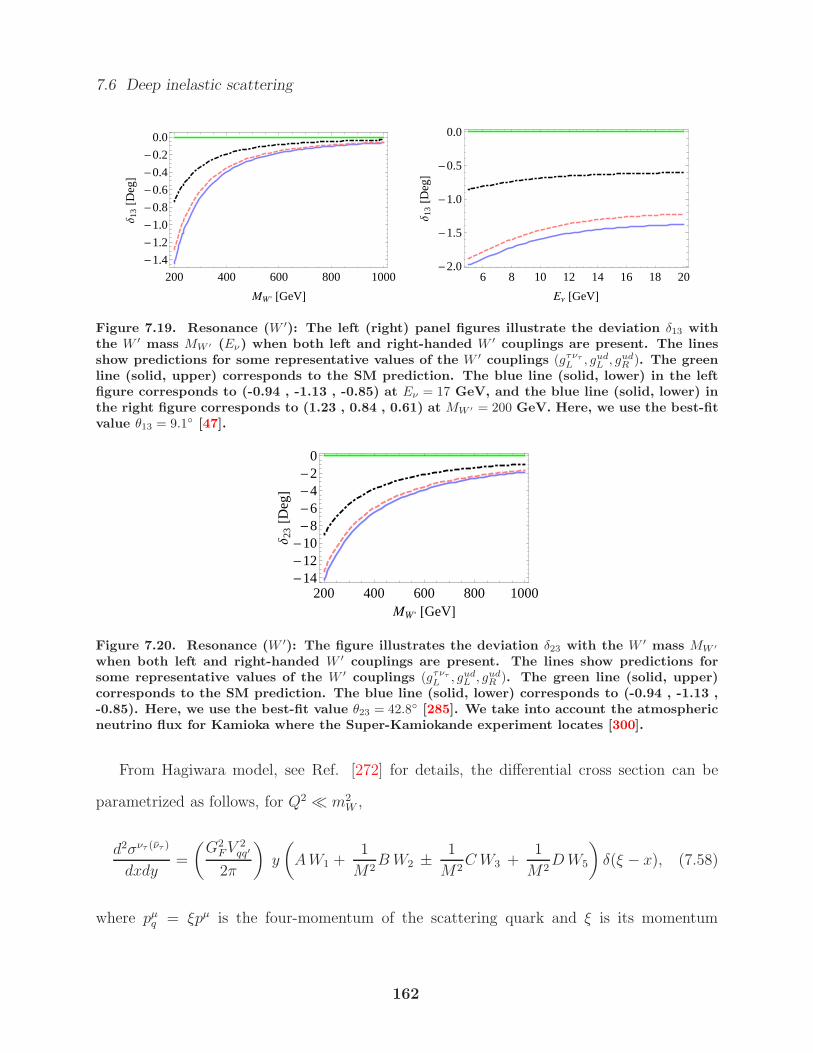
7.6 Deep inelastic scattering
200 400 600 800 1000
-1.4
-1.2
-1.0
-0.8
-0.6
-0.4
-0.2
0.0
MW ' @GeVD
∆13@D
egD
6 8 10 12 14 16 18 20-2.0
-1.5
-1.0
-0.5
0.0
EΝ @GeVD
∆13@D
egD
Figure 7.19. Resonance (W ′): The left (right) panel figures illustrate the deviation δ13 withthe W ′ mass MW ′ (Eν) when both left and right-handed W ′ couplings are present. The linesshow predictions for some representative values of the W ′ couplings (gτντ
L, gud
L, gud
R). The green
line (solid, upper) corresponds to the SM prediction. The blue line (solid, lower) in the leftfigure corresponds to (-0.94 , -1.13 , -0.85) at Eν = 17 GeV, and the blue line (solid, lower) inthe right figure corresponds to (1.23 , 0.84 , 0.61) at MW ′ = 200 GeV. Here, we use the best-fitvalue θ13 = 9.1 [47].
200 400 600 800 1000-14-12-10-8-6-4-2
0
MW ' @GeVD
∆23@D
egD
Figure 7.20. Resonance (W ′): The figure illustrates the deviation δ23 with the W ′ mass MW ′
when both left and right-handed W ′ couplings are present. The lines show predictions forsome representative values of the W ′ couplings (gτντ
L, gud
L, gud
R). The green line (solid, upper)
corresponds to the SM prediction. The blue line (solid, lower) corresponds to (-0.94 , -1.13 ,-0.85). Here, we use the best-fit value θ23 = 42.8 [285]. We take into account the atmosphericneutrino flux for Kamioka where the Super-Kamiokande experiment locates [300].
From Hagiwara model, see Ref. [272] for details, the differential cross section can be
parametrized as follows, for Q2 ≪ m2W ,
d2σντ (ντ )
dxdy=
(G2
FV2qq′
2π
)y
(AW1 +
1
M2BW2 ± 1
M2CW3 +
1
M2DW5
)δ(ξ − x), (7.58)
where pµq = ξpµ is the four-momentum of the scattering quark and ξ is its momentum
162
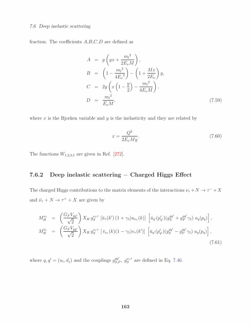
7.6 Deep inelastic scattering
fraction. The coefficients A,B,C,D are defined as
A = y
(yx+
ml2
2EνM
),
B =
(1− ml
2
4Eν2
)−(1 +
Mx
2Eν
)y,
C = 2y
(x(1− y
2
)− ml
2
4EνM
),
D =ml
2
EνM, (7.59)
where x is the Bjorken variable and y is the inelasticity and they are related by
x =Q2
2EνMy. (7.60)
The functions W1,2,3,5 are given in Ref. [272].
7.6.2 Deep inelastic scattering − Charged Higgs Effect
The charged Higgs contributions to the matrix elements of the interactions ντ +N → τ−+X
and ντ +N → τ+ +X are given by
MντH =
(GFVqq′√
2
)XH g
νττS [uτ(k
′) (1 + γ5)uντ (k)][uq′(p
′q′)(g
qq′
S + gqq′
P γ5) uq(pq)],
M ντH =
(GFVqq′√
2
)XH g
νττS [ vντ (k)(1− γ5)vτ (k
′)][uq′(p
′q′)(g
qq′
S − gqq′
P γ5) uq(pq)],
(7.61)
where q, q′ = (ui, dj) and the couplings gqq′
S,P , gνττS are defined in Eq. 7.46.
163
7.6 Deep inelastic scattering
The differential cross section is given by
d2σντ (ντ )
dxdy=
(G2
FV2qq′
2π
)X2
H (gvllS )2 y Lντ (ντ )µν W µν δ(ξ − x)
=
(G2
FV2qq′Eν M
π
)X2
H (gvllS )2[y
(yx+
ml2
2EνM
)]
1
4
[(gqq
′
S )2 + (gqq′
P )2]F1 δ(ξ − x), (7.62)
where XH = M2W/M
2H and the definitions of the 2HDM coupling constants are given in
Eqs. 7.46. There is no interference term of the SM and NP amplitudes. Thus, with the
constraints on the NP parameters (MH , tan β), the charged Higgs contributions relative to
the SM r23H = σH(ντ )/σSM(ντ ) and r13H = σH(ντ )/σSM(ντ ) are small within the kinematical
interval Wcut < W <√s−mτ GeV with Wcut = 1.4 GeV. Thus, the deviations δ23 and δ13
of the mixing angles are negligibly small.
7.6.3 Deep inelastic scattering - W ′ model
The matrix elements are
MντW ′ =
(−iGFVqq′KW ′√2
)[uτ(k
′)γµ(1− γ5)uντ (k)][uq′(p
′q′) γµ (γ
ρW ′ − γκW ′γ5) uq(pq)
],
M ντW ′ =
(−iGFVqq′KW ′√2
)[vντ (k)γ
µ(1− γ5)vτ (k′)]
[uq′(p
′q′) γµ (γ
ρW ′ − γκW ′γ5) uq(pq)
],
(7.63)
164
7.6 Deep inelastic scattering
where the definitions are
γρW ′ = XW ′gνττL (gqq′
L + gqq′
R ),
γκW ′ = XW ′gνττL (gqq′
L − gqq′
R ),
XW ′ =
(m2
W
m2W ′
),
KW ′ =
(1 +
Q2
m2W ′
)−1
. (7.64)
The total differential cross section has the same form as the SM one in Eq. (7.58), after
setting K2W ′ ∼ 1,
d2σντ (ντ )SM+W ′
dxdy=
(G2
FV2qq′
2π
)y
(A′W1 +
1
M2B′W2 ± 1
M2C ′W3 +
1
M2D′W5
)δ(ξ − x),
(7.65)
where A′,B′,C ′, and D′ are defined as:
A′ =1
2A(|a′|2 + |b′|2
),
B′ =1
2B(|a′|2 + |b′|2
),
C ′ = Re[a′b′∗]C,
D′ =1
2D
(|a′|2 + |b′|2
). (7.66)
with
a′ = 1 + γρW ′,
b′ = 1 + γκW ′. (7.67)
The ratios of theW ′ contributions to the SM cross sections r23W ′ and r13W ′ and the deviations
δ23 and δ13 are shown within the allowed kinematical range M + mπ < W < 1.4 GeV in
165
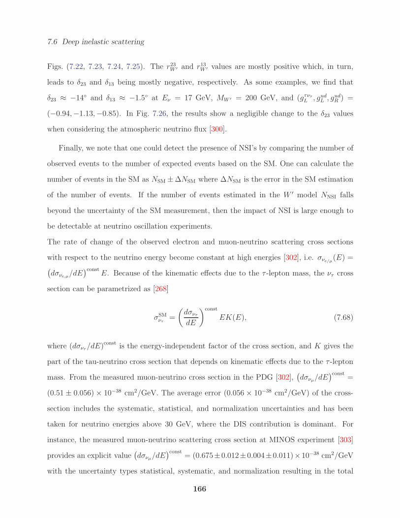
7.6 Deep inelastic scattering
Figs. (7.22, 7.23, 7.24, 7.25). The r23W ′ and r13W ′ values are mostly positive which, in turn,
leads to δ23 and δ13 being mostly negative, respectively. As some examples, we find that
δ23 ≈ −14 and δ13 ≈ −1.5 at Eν = 17 GeV, MW ′ = 200 GeV, and (gτντL , gudL , gudR ) =
(−0.94,−1.13,−0.85). In Fig. 7.26, the results show a negligible change to the δ23 values
when considering the atmospheric neutrino flux [300].
Finally, we note that one could detect the presence of NSI’s by comparing the number of
observed events to the number of expected events based on the SM. One can calculate the
number of events in the SM as NSM ±∆NSM where ∆NSM is the error in the SM estimation
of the number of events. If the number of events estimated in the W ′ model NNSI falls
beyond the uncertainty of the SM measurement, then the impact of NSI is large enough to
be detectable at neutrino oscillation experiments.
The rate of change of the observed electron and muon-neutrino scattering cross sections
with respect to the neutrino energy become constant at high energies [302], i.e. σνe/µ(E) =(dσνe,µ/dE
)constE. Because of the kinematic effects due to the τ -lepton mass, the ντ cross
section can be parametrized as [268]
σSMντ =
(dσντdE
)const
EK(E), (7.68)
where (dσντ/dE)const is the energy-independent factor of the cross section, and K gives the
part of the tau-neutrino cross section that depends on kinematic effects due to the τ -lepton
mass. From the measured muon-neutrino cross section in the PDG [302],(dσνµ/dE
)const=
(0.51 ± 0.056)× 10−38 cm2/GeV. The average error (0.056 × 10−38 cm2/GeV) of the cross-
section includes the systematic, statistical, and normalization uncertainties and has been
taken for neutrino energies above 30 GeV, where the DIS contribution is dominant. For
instance, the measured muon-neutrino scattering cross section at MINOS experiment [303]
provides an explicit value(dσνµ/dE
)const= (0.675±0.012±0.004±0.011)×10−38 cm2/GeV
with the uncertainty types statistical, systematic, and normalization resulting in the total
166

7.6 Deep inelastic scattering
uncertainty 0.018 for the energy range 30-50 GeV ( the MINOS results are included in
the average value). Since we consider the NP contributions in the tau sector only, we can
take the energy-independent factor of the SM tau-neutrino cross section to be given as
(dσντ/dE)const =
(dσνµ/dE
)constbecause of the SM universality of the weak interactions.
The uncertainty of the number of ντ events calculated in the SM limit follow from the
uncertainty of (dσντ/dE)const.
The number of tau-neutrino events in the SM is found to be NSM = 30.66 ± 3.37 using
the PDG cross section value for the 22.5 kton fiducial volume of the Super-K detector [265]
during the 2806 day running period. The atmospheric neutrino flux [301] has been taken for
vertically upward going neutrinos (cos θ = −1) where θ is the zenith angle. The distance d
traveled by atmospheric neutrinos can be calculated by [301]
d =√
(h2 + 2Reh) + (Re cos θ)2 − Re cos θ, (7.69)
where h is the neutrino production height and Re is the radius of the earth - its surface is
assumed to be spherical. In Ref. [301] there is a distribution for the atmospheric neutrino
flux at a zenith angle around (cos θ = 1). Since the distribution of the flux over the zenith
angle is symmetric at high neutrino energy, see [273], the flux is the same at cos θ = −1
and 1. We choose to work with cos θ = −1 because the distance d will be maximum,
through the diameter of the earth, which in turns enhances the transition probability We
take h = 4.5 × 10⁴ m for the accumulated probability of 99% for the vertical production
height [301] and we integrate over the neutrino energies from 30− 100 GeV.
Next we calculate the number of events in theW ′ model in the DIS energy region ignoring
the QE and ∆-RES contributions. In order to cross-check our calculations we find the SM
number of events to be NSM = 30.08 by setting the couplings (gνττL , gudL , gudR ) = (0, 0, 0) which
is very close to NSM estimated above. In Fig. 7.21, we show the contour plot for the number
167
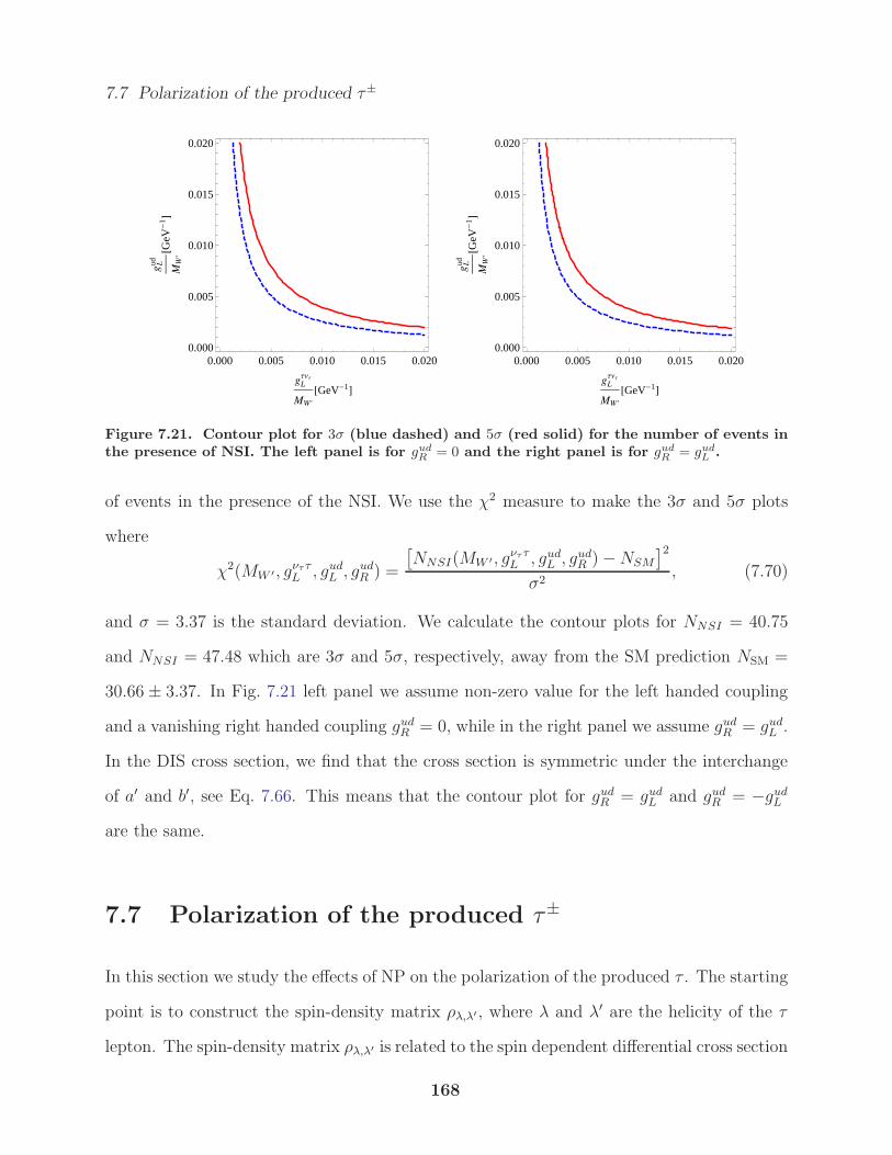
7.7 Polarization of the produced τ±
0.000 0.005 0.010 0.015 0.0200.000
0.005
0.010
0.015
0.020
gLΤΝΤ
MW '
@GeV-1D
gLud
MW
'@G
eV-
1 D
0.000 0.005 0.010 0.015 0.0200.000
0.005
0.010
0.015
0.020
gLΤΝΤ
MW '
@GeV-1D
gLud
MW
'@G
eV-
1 D
Figure 7.21. Contour plot for 3σ (blue dashed) and 5σ (red solid) for the number of events inthe presence of NSI. The left panel is for gud
R= 0 and the right panel is for gud
R= gud
L.
of events in the presence of the NSI. We use the χ2 measure to make the 3σ and 5σ plots
where
χ2(MW ′, gνττL , gudL , gudR ) =
[NNSI(MW ′, gνττL , gudL , g
udR )−NSM
]2
σ2, (7.70)
and σ = 3.37 is the standard deviation. We calculate the contour plots for NNSI = 40.75
and NNSI = 47.48 which are 3σ and 5σ, respectively, away from the SM prediction NSM =
30.66 ± 3.37. In Fig. 7.21 left panel we assume non-zero value for the left handed coupling
and a vanishing right handed coupling gudR = 0, while in the right panel we assume gudR = gudL .
In the DIS cross section, we find that the cross section is symmetric under the interchange
of a′ and b′, see Eq. 7.66. This means that the contour plot for gudR = gudL and gudR = −gudLare the same.
7.7 Polarization of the produced τ±
In this section we study the effects of NP on the polarization of the produced τ . The starting
point is to construct the spin-density matrix ρλ,λ′ , where λ and λ′ are the helicity of the τ
lepton. The spin-density matrix ρλ,λ′ is related to the spin dependent differential cross section
168
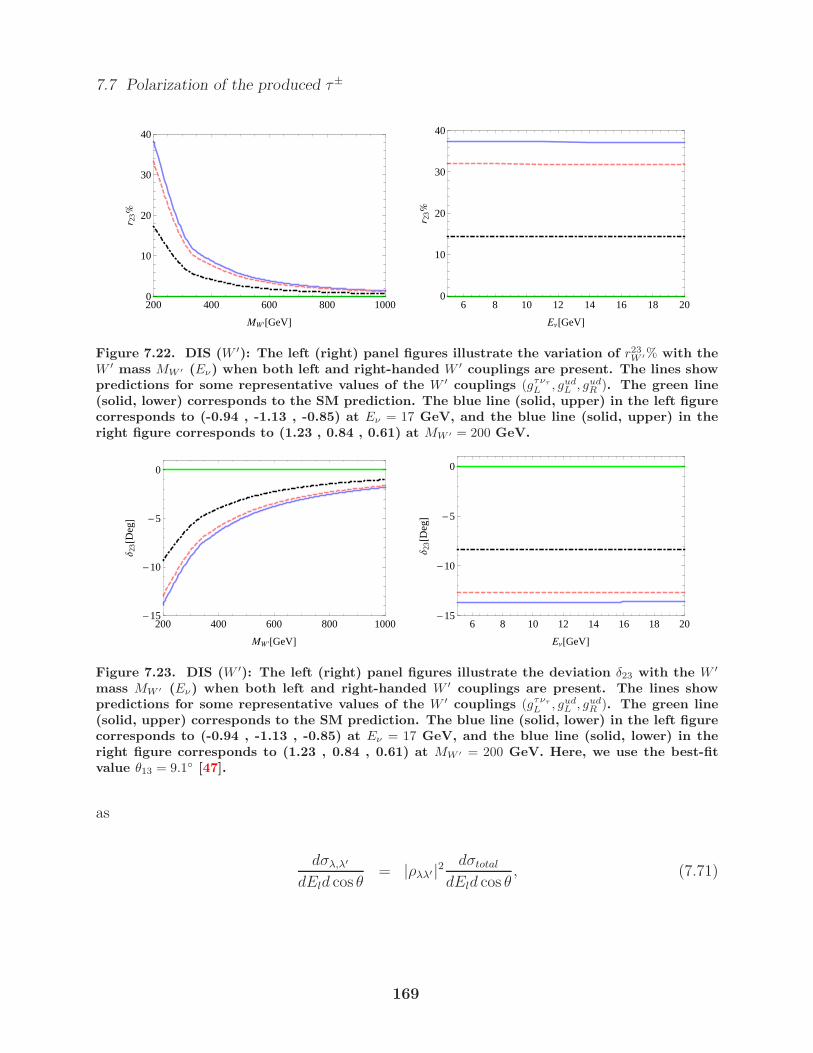
7.7 Polarization of the produced τ±
200 400 600 800 10000
10
20
30
40
MW '@GeVD
r 23%
6 8 10 12 14 16 18 200
10
20
30
40
EΝ@GeVD
r 23%
Figure 7.22. DIS (W ′): The left (right) panel figures illustrate the variation of r23W ′% with the
W ′ mass MW ′ (Eν) when both left and right-handed W ′ couplings are present. The lines showpredictions for some representative values of the W ′ couplings (gτντ
L, gud
L, gud
R). The green line
(solid, lower) corresponds to the SM prediction. The blue line (solid, upper) in the left figurecorresponds to (-0.94 , -1.13 , -0.85) at Eν = 17 GeV, and the blue line (solid, upper) in theright figure corresponds to (1.23 , 0.84 , 0.61) at MW ′ = 200 GeV.
200 400 600 800 1000-15
-10
-5
0
MW '@GeVD
∆23@D
egD
6 8 10 12 14 16 18 20-15
-10
-5
0
EΝ@GeVD
∆23@D
egD
Figure 7.23. DIS (W ′): The left (right) panel figures illustrate the deviation δ23 with the W ′
mass MW ′ (Eν) when both left and right-handed W ′ couplings are present. The lines showpredictions for some representative values of the W ′ couplings (gτντ
L, gud
L, gud
R). The green line
(solid, upper) corresponds to the SM prediction. The blue line (solid, lower) in the left figurecorresponds to (-0.94 , -1.13 , -0.85) at Eν = 17 GeV, and the blue line (solid, lower) in theright figure corresponds to (1.23 , 0.84 , 0.61) at MW ′ = 200 GeV. Here, we use the best-fitvalue θ13 = 9.1 [47].
as
dσλ,λ′
dEld cos θ= |ρλλ′ |2 dσtotal
dEld cos θ, (7.71)
169
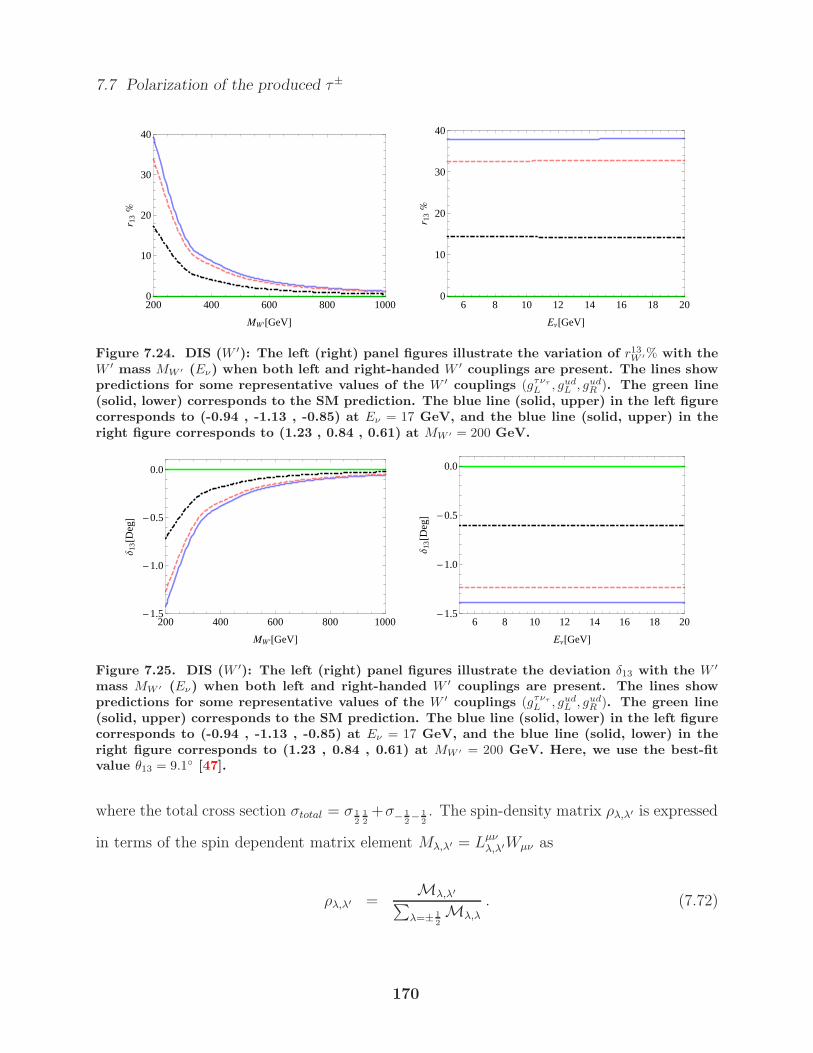
7.7 Polarization of the produced τ±
200 400 600 800 10000
10
20
30
40
MW '@GeVD
r 13%
6 8 10 12 14 16 18 200
10
20
30
40
EΝ@GeVD
r 13%
Figure 7.24. DIS (W ′): The left (right) panel figures illustrate the variation of r13W ′% with the
W ′ mass MW ′ (Eν) when both left and right-handed W ′ couplings are present. The lines showpredictions for some representative values of the W ′ couplings (gτντ
L, gud
L, gud
R). The green line
(solid, lower) corresponds to the SM prediction. The blue line (solid, upper) in the left figurecorresponds to (-0.94 , -1.13 , -0.85) at Eν = 17 GeV, and the blue line (solid, upper) in theright figure corresponds to (1.23 , 0.84 , 0.61) at MW ′ = 200 GeV.
200 400 600 800 1000-1.5
-1.0
-0.5
0.0
MW '@GeVD
∆13@D
egD
6 8 10 12 14 16 18 20-1.5
-1.0
-0.5
0.0
EΝ@GeVD
∆13@D
egD
Figure 7.25. DIS (W ′): The left (right) panel figures illustrate the deviation δ13 with the W ′
mass MW ′ (Eν) when both left and right-handed W ′ couplings are present. The lines showpredictions for some representative values of the W ′ couplings (gτντ
L, gud
L, gud
R). The green line
(solid, upper) corresponds to the SM prediction. The blue line (solid, lower) in the left figurecorresponds to (-0.94 , -1.13 , -0.85) at Eν = 17 GeV, and the blue line (solid, lower) in theright figure corresponds to (1.23 , 0.84 , 0.61) at MW ′ = 200 GeV. Here, we use the best-fitvalue θ13 = 9.1 [47].
where the total cross section σtotal = σ 12
12+σ− 1
2− 1
2. The spin-density matrix ρλ,λ′ is expressed
in terms of the spin dependent matrix element Mλ,λ′ = Lµνλ,λ′Wµν as
ρλ,λ′ =Mλ,λ′∑
λ=± 1
2
Mλ,λ
. (7.72)
170
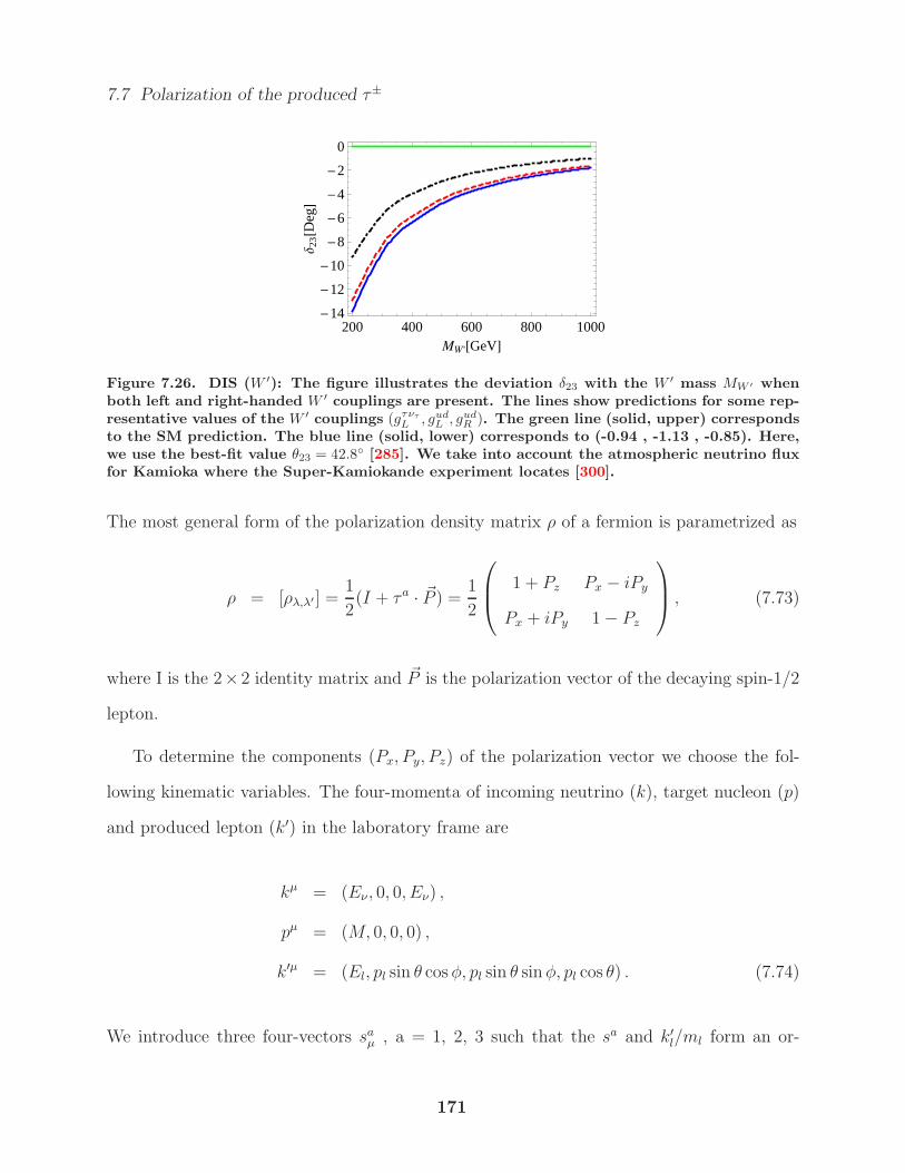
7.7 Polarization of the produced τ±
200 400 600 800 1000-14
-12
-10
-8
-6
-4
-2
0
MW '@GeVD
∆23@D
egD
Figure 7.26. DIS (W ′): The figure illustrates the deviation δ23 with the W ′ mass MW ′ whenboth left and right-handed W ′ couplings are present. The lines show predictions for some rep-resentative values of the W ′ couplings (gτντ
L, gud
L, gud
R). The green line (solid, upper) corresponds
to the SM prediction. The blue line (solid, lower) corresponds to (-0.94 , -1.13 , -0.85). Here,we use the best-fit value θ23 = 42.8 [285]. We take into account the atmospheric neutrino fluxfor Kamioka where the Super-Kamiokande experiment locates [300].
The most general form of the polarization density matrix ρ of a fermion is parametrized as
ρ = [ρλ,λ′ ] =1
2(I + τa · ~P ) = 1
2
1 + Pz Px − iPy
Px + iPy 1− Pz
, (7.73)
where I is the 2×2 identity matrix and ~P is the polarization vector of the decaying spin-1/2
lepton.
To determine the components (Px, Py, Pz) of the polarization vector we choose the fol-
lowing kinematic variables. The four-momenta of incoming neutrino (k), target nucleon (p)
and produced lepton (k′) in the laboratory frame are
kµ = (Eν , 0, 0, Eν) ,
pµ = (M, 0, 0, 0) ,
k′µ = (El, pl sin θ cosφ, pl sin θ sinφ, pl cos θ) . (7.74)
We introduce three four-vectors saµ , a = 1, 2, 3 such that the sa and k′l/ml form an or-
171
7.7 Polarization of the produced τ±
thonormal set of four-vectors as defined in [304]: We choose the three spin four-vectors of
the lepton such that
sa · k′ = 0,
sa · sb = −δab,
saµ · sbν = −gµν +k′µk
′ν
m2l
, (7.75)
where
s1µ = (0, cos θ cosφ, cos θ sinφ,− sin θ) ,
s2µ = (0,− sinφ, cosφ, 0) ,
s3µ = (pl/ml, El/ml sin θ cos φ,El/ml sin θ sinφ,El/ml cos θ) . (7.76)
Finally we define the degree of τ polarization P as
P =√P 2x + P 2
y + P 2z . (7.77)
The SM results for the polarization components Px, Py, Pz can be found in Ref. [272] for
the processes QE, ∆-RES and DIS. We calculated these components in the presence of the
charged Higgs and W ′ contributions. We computed the degree of τ polarization P with
respect to Eτ for 0 degree, 5 degrees and 10 degrees scattering angles with the incident
neutrino energy at 10 GeV. In the polarization results we found the charged Higgs and W ′
model produce tiny deviations from the SM values.
172
7.8 Conclusion
7.8 Conclusion
In this work we calculated the effect of a charged Higgs and a W ′ contribution to ντ +N →
τ−+X and ντ +N → τ++X scattering. We constrained the parameters of both the models
from τ− → π−ντ and τ− → ρ−ντ decays. Corrections to the SM contribution to ντ +N →
τ−+X and ντ+N → τ++X impact the extraction of the neutrino atmospheric mixing angles
θ23 and θ13, respectively. We found that the charged Higgs model can produce significant
corrections to δ23,13 that measure the deviation of the actual θ23,13 from the (θ23,13)SM angles
which are extracted assuming the SM ντ/ντ scattering cross sections.
In quasielastic scattering, the W ′ model effect generates a large deviation δ23 but negligi-
bly small δ13. As θ13 is smaller than θ23 larger NP in ντ + p→ τ+ +n is required to produce
effects in δ13 similar in size to δ23. When a charged Higgs is involved, δ23,13 are negative. This
is because there is no interference of the charged Higgs contribution with the SM contribu-
tion, for massless neutrinos, and so the cross sections for ντ+n→ τ−+p and ντ+p→ τ++n
are always larger than the SM cross sections. This means that experiments should measure
θ23,13 larger than the present values in the presence of a charged Higgs contribution. In this
case we also found that δ23,13 increase in magnitude with the neutrino energy. Hence, a pos-
sible sign of the charged Higgs effect would be a measurement of θ23,13 that shows an increase
with increasing neutrino energy. For the W ′ model we calculated a significant contribution
to δ23 which can be both positive and negative, but is mostly negative. The deviation δ23
was found to be independent of the neutrino energy for a left-handedW ′ but neutrino energy
dependent when both left- and right-handed W ′ chiralities were present. A negligibly small
deviation, δ13, was found in the W ′ model because of the small value of θ13.
In the case of ∆ resonance production, the charged Higgs contribution was found to be
proportional to q2 which suppressed the NP effect within the allowed kinematical region.
The values of the deviations δ23 and δ13 were negative as the interference term in the cross
173
7.8 Conclusion
section vanishes in the limit of ignoring the neutrino mass and, in turn, the total cross
section is always larger than the SM one. The values of δ23 and δ13 in the W ′ gauge boson
contributions were found to be both positive and negative, but were mostly negative. The
δ23 and δ13 values decreased in magnitude with increasing incident neutrino energy and the
new state masses (MW ′,MH).
In the case of deep inelastic scattering, the charged Higgs contribution does not have
interference with the SM cross section. With the constraints on the NP parameters, the NP
effects were negligible and the deviations δ23 and δ13 were very small. The values of deviations
were found to be mostly negative in the W ′ model. The δ23 and δ13 values increased in
magnitude with increasing incident neutrino energy and decreased with increasing MW ′.
We took into account the flux of incoming atmospheric neutrinos from Kamioka, where
the Super-Kamiokande experiment is located, in the calculations of δ23 when considering
the charged Higgs and W ′ contributions. By integrating over the incoming neutrino energy
we found that considering the neutrino flux did not change the δ23 results significantly. We
showed the 3σ and 5σ deviation contour plots, using the χ2 measure and the W ′ NSI model,
for the number of events for neutrino energies above 30 GeV where the DIS contribution is
dominant. Finally, we studied the NP effects on the degree of polarization of the produced
τ and found that the deviation of the polarization results in the NP models from the SM
values were negligibly small at different scattering angles.
We have presented in this work a first estimation of the charged Higgs and W ′ effects
in the extraction of θ23 and θ13. We hope more detailed calculations including nuclear as
well as detector effects, will be done to find out whether these new physics effects can be
observed at present ντ/ντ appearance experiments and/or to motivate new experiments that
can detect these effects.
174
Overall Conclusion
In this dissertation, we presented a study of the phenomenological implications of two-Higgs-
doublet model on the properties of neutrino sector and heavy quark systems. We discussed
neutrino mixing within the framework of two-Higgs-doublet model by introducing different
flavor symmetries in the lepton sector with the leading order structures being bi-maximal
and tri-bimaximal pattern. We found that a mixing model with 2-3 flavor symmetry can ac-
commodate the sizable θ13 value. Moreover, we introduced a model with A4 flavor symmetry
where the smallness of the neutrino mass is not due to the seesaw mechanism, i.e. not in-
versely proportional to some large mass scale, at the level of a one-loop mechanism with dark
matter in the loop consisting of singlet Majorana fermions. In the nonstandard neutrino in-
teractions, new physics contributions to the tau-neutrino nucleon scattering were considered
in this work. We discussed charged Higgs and W ′ effects to the three processes; quasi-elastic
interaction, ∆ resonance production and deep inelastic scattering in the neutrino-nucleon in-
teractions ντ +N → τ−+X and ντ +N → τ++X . Considering these effects in the neutrino
detection process at neutrino oscillation experiments modifies the measured atmospheric and
reactor mixing angles θ23 and θ13, respectively.
We studied the decay channel of the quarkonium ηb → τ+τ− which has an experimental
upper limit of . 8% on its branching ratio. We evaluated the standard model branching
ratio for this decay to be ∼ 4 × 10⁻⁹. We showed that the contributions of models with a
light pseudoscalar or a light axial vector state enhance the branching ratio up to the present
175
experimental limit. In the top sector, the forward-backward asymmetry AFB in the top quark
pair production in the tt rest frame has been measured in the CDF and found to have a
deviation from the next-to leading order SM prediction. Here, we accommodated the CDF
measurement of the AFB by introducing a u → t transition via a flavor-changing Z ′ which
can explain the data. We considered the most general form of the tuZ ′ interaction, which
includes vector-axial vector as well as tensor type couplings, and studied how these couplings
affect the top forward-backward asymmetry.
176
Appendix 1
Majorana Field
A.1 Weyl spinor
In physics, a Majorana fermion is a fermion which is its own anti-particle. This definition
refers to the Majorana condition ψ = ψc where ψc is the charge conjugate field. No Majorana
fermions are known in nature as elementary particles. The neutrino might be a Majorana
fermion or it might be a Dirac fermion. If it is a Majorana fermion, then neutrinoless
double beta decay is possible; experiments are underway to search for this. The hypothet-
ical neutralino of supersymmetric models is a Majorana fermion. The charge conjugation
transformation is defined as
ψc = CψT , (A.1)
where C is the charge conjugation operator.
There are different kinds of matrix representations for the charge conjugation operator.
The one we will use in here is
C = −iγ2γ0. (A.2)
In this representation, the C matrix is independent of the basis. In the following we will use
177
A.1 Weyl spinor
the Weyl (Chiral) basis to take a closer look at C.
C = −iγ2γ0
= −i
0 σ2
−σ2 0
0 1
1 0
=
0 −1 0 0
1 0 0 0
0 0 0 1
0 0 −1 0
. (A.3)
There are some basic properties of the C matrix
C† = CT = C−1 = −C,
C−1γµC = −γT ,
C−1γ5C = γ5 = γT5 . (A.4)
Under Lorentz transformation, the field function is transformed as follows
ψ′c = S(Λ)ψc, (A.5)
where S(Λ) is the Lorentz transformation matrix. Now, we want to find the explicit form of
the Lorentz operator. Pure ‘boost’ Lorentz transformations are those connecting two inertial
frames, moving with relative speed v. Pure Lorentz transformations can be parameterized
178
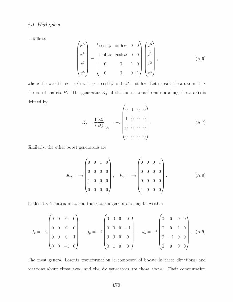
A.1 Weyl spinor
as follows
x0′
x1′
x2′
x3′
=
coshφ sinh φ 0 0
sinh φ coshφ 0 0
0 0 1 0
0 0 0 1
x0
x1
x2
x3
, (A.6)
where the variable φ = v/c with γ = cosh φ and γβ = sinhφ. Let us call the above matrix
the boost matrix B. The generator Kx of this boost transformation along the x axis is
defined by
Kx =1
i
∂B
∂φ
∣∣∣∣φ0
= −i
0 1 0 0
1 0 0 0
0 0 0 0
0 0 0 0
. (A.7)
Similarly, the other boost generators are
Ky = −i
0 0 1 0
0 0 0 0
1 0 0 0
0 0 0 0
, Kz = −i
0 0 0 1
0 0 0 0
0 0 0 0
1 0 0 0
. (A.8)
In this 4× 4 matrix notation, the rotation generators may be written
Jx = −i
0 0 0 0
0 0 0 0
0 0 0 1
0 0 −1 0
, Jy = −i
0 0 0 0
0 0 0 −1
0 0 0 0
0 1 0 0
, Jz = −i
0 0 0 0
0 0 1 0
0 −1 0 0
0 0 0 0
. (A.9)
The most general Lorentz transformation is composed of boosts in three directions, and
rotations about three axes, and the six generators are those above. Their commutation
179
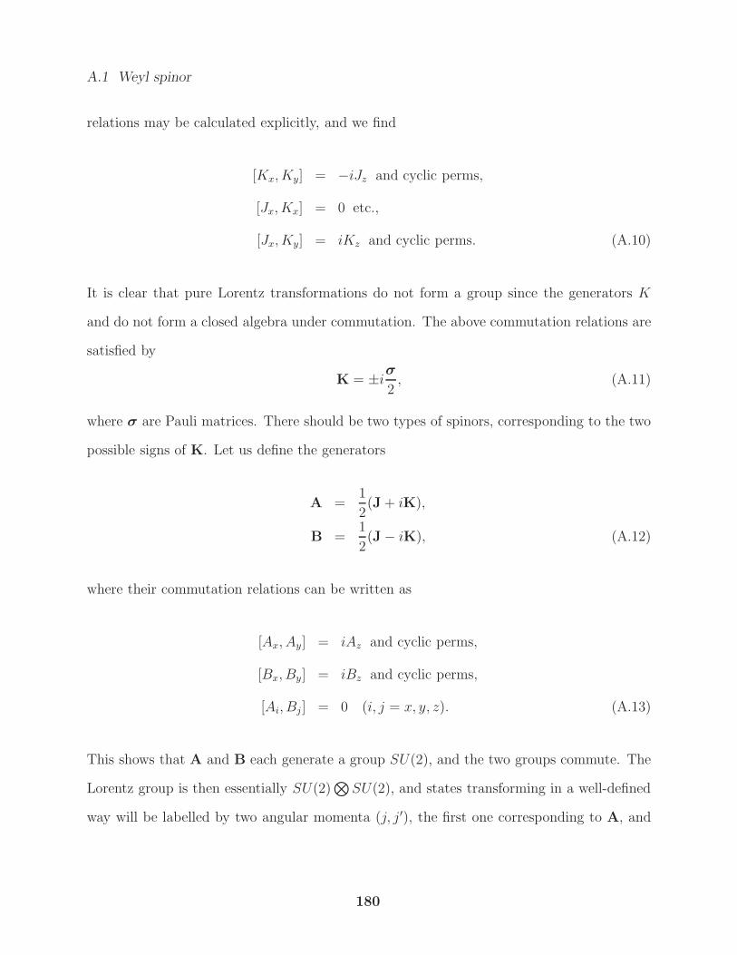
A.1 Weyl spinor
relations may be calculated explicitly, and we find
[Kx, Ky] = −iJz and cyclic perms,
[Jx, Kx] = 0 etc.,
[Jx, Ky] = iKz and cyclic perms. (A.10)
It is clear that pure Lorentz transformations do not form a group since the generators K
and do not form a closed algebra under commutation. The above commutation relations are
satisfied by
K = ±iσ2, (A.11)
where σ are Pauli matrices. There should be two types of spinors, corresponding to the two
possible signs of K. Let us define the generators
A =1
2(J+ iK),
B =1
2(J− iK), (A.12)
where their commutation relations can be written as
[Ax, Ay] = iAz and cyclic perms,
[Bx, By] = iBz and cyclic perms,
[Ai, Bj ] = 0 (i, j = x, y, z). (A.13)
This shows that A and B each generate a group SU(2), and the two groups commute. The
Lorentz group is then essentially SU(2)⊗
SU(2), and states transforming in a well-defined
way will be labelled by two angular momenta (j, j′), the first one corresponding to A, and
180
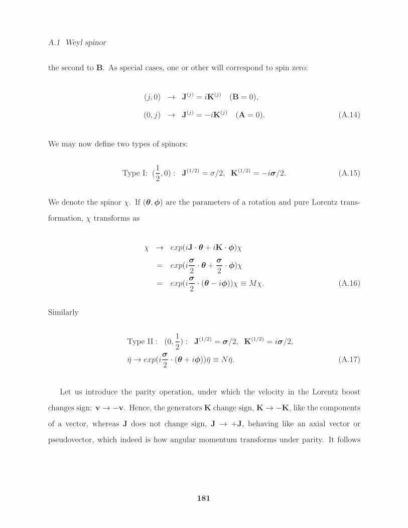
A.1 Weyl spinor
the second to B. As special cases, one or other will correspond to spin zero:
(j, 0) → J(j) = iK(j) (B = 0),
(0, j) → J(j) = −iK(j) (A = 0). (A.14)
We may now define two types of spinors:
Type I: (1
2, 0) : J(1/2) = σ/2, K(1/2) = −iσ/2. (A.15)
We denote the spinor χ. If (θ,φ) are the parameters of a rotation and pure Lorentz trans-
formation, χ transforms as
χ → exp(iJ · θ + iK · φ)χ
= exp(iσ
2· θ +
σ
2· φ)χ
= exp(iσ
2· (θ − iφ))χ ≡Mχ. (A.16)
Similarly
Type II : (0,1
2) : J(1/2) = σ/2, K(1/2) = iσ/2,
η → exp(iσ
2· (θ + iφ))η ≡ Nη. (A.17)
Let us introduce the parity operation, under which the velocity in the Lorentz boost
changes sign: v → −v. Hence, the generators K change sign, K → −K, like the components
of a vector, whereas J does not change sign, J → +J, behaving like an axial vector or
pseudovector, which indeed is how angular momentum transforms under parity. It follows
181
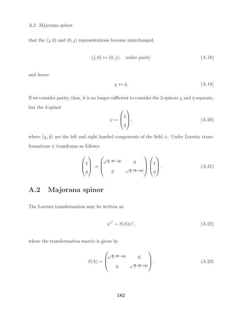
A.2 Majorana spinor
that the (j, 0) and (0, j) representations become interchanged,
(j, 0) ↔ (0, j), under parity (A.18)
and hence
χ↔ η. (A.19)
If we consider parity, then, it is no longer sufficient to consider the 2-spinors χ and η separate,
but the 4-spinor
ψ =
χ
η
, (A.20)
where (χ, η) are the left and right handed components of the field ψ. Under Lorentz trans-
formations ψ transforms as follows:
χ
η
→
ei
σ
2·(θ−iφ) 0
0 eiσ
2·(θ+iφ)
χ
η
. (A.21)
A.2 Majorana spinor
The Lorentz transformation may be written as
ψc′ = S(Λ)ψc, (A.22)
where the transformation matrix is given by
S(Λ) =
ei
σ
2·(θ−iφ) 0
0 eiσ
2·(θ+iφ)
. (A.23)
182
A.2 Majorana spinor
From the above equation
S ≡ eiσ
2(θ−iφ), (A.24)
S−1 ≡ e−iσ2(θ−iφ), (A.25)
S−1† ≡ eiσ
2(θ+iφ), (A.26)
S(Λ) =
S 0
0 S−1†
. (A.27)
Thus, under Lorentz transformations
χ→ Sχ, η → S−1†η (A.28)
We want to construct Lorentz invariant terms out of the spinors χ, η
χ-Field
Under Lorentz transformation
χ → χ′ ≡ Sχ,
(iσ(2)χ) → (iσ(2)χ′) ≡ (iσ(2)Sχ). (A.29)
Since
σ(2)σTσ(2) = −σ. (A.30)
183
A.2 Majorana spinor
Thus,
σ(2)Sσ(2) = σ(2)ei2σ(θ−iφ)σ(2)
= e−i2σT (θ−iφ)
= S−1T , (A.31)
or
σ(2)S∗σ(2) = S−1†. (A.32)
We see that S∗ and S−1† are equivalent representations of the Lorentz group. Under Lorentz
transformation
(iσ(2)χ) → iσ(2)χ′
= iσ(2)Sχ
= S−1T (iσ(2)χ), (A.33)
hence
(iσ(2)χ)T → (iσ(2)χ)TS−1, (A.34)
which together with Eq. A.29 implies that
(iσ(2)χ)Tχ is Lorentz invariant. (A.35)
Now let us give explicit indicies to the spinor χ. We put
χ ≡ χα =
χ1
χ2
. (A.36)
184
A.2 Majorana spinor
We further put
χ1
χ2
≡ χα = (iσ(2)χ) =
0 1
−1 0
χ1
χ2
=
χ2
−χ1
, (A.37)
which leads to
χαTχα is Lorentz invariant. (A.38)
η- Field
Under Lorentz transformation
η → η′ ≡ S−1†η, (A.39)
then
(−iσ(2)η) → (−iσ(2)η′)
= −iσ(2)S−1†η
= S∗(−iσ(2)η), (A.40)
or
(−iσ(2)η)T → (−iσ(2)η)TS†. (A.41)
Here we have used the relation A.32. Thus
(−iσ(2)η)T η is Lorentz invariant. (A.42)
185
A.2 Majorana spinor
Now let us give explicit indicies to the spinor χ. We put
η ≡ ηα =
η1
η2
. (A.43)
We further put
η1
η2
≡ ηα = (−iσ(2)η) =
0 −1
1 0
η1
η2
=
−η2
η1
, (A.44)
which leads to
ηTα ηα is Lorentz invariant. (A.45)
Now, we have four types of Weyl spinors:
χα, χα, χα, χ
α, (A.46)
where we simply rename the spinors
χα ≡ ηα, and χα ≡ ηα. (A.47)
It is common to refer to these types as dotted and undotted spinors. The relationship
between them is not hard to deduce. From Eqs. (A.28, A.33, A.40) we have the following
transformation property for the spinors under a Lorentz transformation
χα → χ′α = Sβ
αχβ
χα → χ′α = (S−1T )αβχβ. (A.48)
186
A.3 Majorana condition
and
χα → χ′α = (S−1†)αβχβ
χα → χ′α = S∗δ
α χ′δ. (A.49)
Comparing Eqs. (A.48, A.49), we are justified in identifying dotted spinors with the complex
conjugate of undeotted ones:
χα = (χα)∗, χα = (χα)∗. (A.50)
A.3 Majorana condition
Putting in spinor indices we have from Eqs. (A.20, A.47), using Eq. A.50,
ψ =
χα
ηα
⇒ ψ† = (χα ηα) ⇒ ψ = ψ†γ0 = (ηα χα) ⇒ ψT =
ηα
χα
. (A.51)
Hence, using Eq. A.3
ψc = CψT = ηc
−σ(2)ηα
σ(2)χα
=
ηα
χα
, (A.52)
where we have chosen ηc = i. Then the Majorana condition ψ = ψc leads to
η = χ, (A.53)
187
A.4 Majorana Lagrangian
hence
ψ = ψc =
χα
χα
=
χα
(χα)∗
(A.54)
A.4 Majorana Lagrangian
The Dirac Lagrangian of fermions is given by
L =1
2iψγµ∂µψ − 1
2mψψ + h.c. (A.55)
The complex conjugate field
ψc = CψT ⇒ ψT = C−1ψc ⇒ ψ = ψcT (C−1)T . (A.56)
Using the Majorana condition
ψ = ψT (C−1)T , (A.57)
then
ψ = −ψTC−1. (A.58)
Thus, the mass term is given by
1
2mψψ =
1
2m
(−ψTC−1
)ψ
= −1
2mψTC−1ψ. (A.59)
188
A.4 Majorana Lagrangian
The kinetic term is given by
1
2iψγµ∂µψ =
1
2i(−ψTC−1
)γµ∂µψ
= −1
2iψTC−1γµ∂µψ. (A.60)
Using Eqs. (A.59, A.60), the Majorana Lagrangian is written as
L = −1
2iψTC−1γµ∂µψ +
1
2mψTC−1ψ + h.c.
= −1
2i(ψTLC
−1γµ∂µψL + ψTRC
−1γµ∂µψR
)
+1
2m
(ψTLC
−1ψL + ψTRC
−1ψR
)+ h.c. (A.61)
The above Lagrangian shows that the Majorana mass term can be composed from either
left- or right-handed components. We want to check the hermitian conjugate term in the
Lagrangian. For example, we will check the hermitian conjugate of ψTRC
−1ψR
(ψTRC
−1ψR
)†= ψ†
R(C−1)†(ψT
R)†
= (ψ∗R)
T (−C)†ψ∗R
= −(ψ∗R)
TCTψ∗R. (A.62)
Using the Majorana condition
ψ = CψT
= C(ψ†γ0)T
= Cγ0ψ∗. (A.63)
189
A.5 Canonical quantization of spinor fields
Substitute in the above equation
−(ψ∗R)
TCTψ∗R = −(γ0C
−1ψR)TCT (γ0C
−1ψR)
= −ψTR(C
−1)Tγ0CT (γ0C
−1ψR)
= ψTRC
−1γ0C−1γ0C
−1ψR
= −ψTRCγ0C
−1γ0C−1ψR
= ψTRγ0γ0C
−1ψR
= ψTRC
−1ψR. (A.64)
That means the hermitian conjugate of the Lagrangian is similar to itself.
A.5 Canonical quantization of spinor fields
The general solution of the Dirac equation is:
ψ(x) =∑
s=±
∫d3p
(2π)32ω
[bs(p)us(p)e
ip·x + d†s(p)vs(p)e−ip·x] ,
ψ(x) =∑
s=±
∫d3p
(2π)32ω
[b†s(p)us(p)e
−ip·x + ds(p)vs(p)eip·x] ,
Cψ(x)T =∑
s=±
∫d3p
(2π)32ω
[b†s(p)Cu
Ts (p)e
−ip·x + ds(p)CvTs (p)e
ip·x] . (A.65)
Let us assume that
CuTs (p) = vs(p),
CvTs (p) = us(p). (A.66)
190
A.5 Canonical quantization of spinor fields
Then
ψc = Cψ(x)T =∑
s=±
∫d3p
(2π)32ω
[b†s(p)vs(p)e
−ip·x + ds(p)us(p)eip·x] . (A.67)
Using the Majorana condition, then
bs(p) = ds(p), (A.68)
thus
ψ = ψc =∑
s=±
∫d3p
(2π)32ω
[bs(p)us(p)e
ip·x + b†s(p)vs(p)e−ip·x] . (A.69)
Now, we want to prove Eqs. A.66. The four-component spinors us(p) and vs(p) obey the
equations
( 6p+m)us(p) = 0,
(−6p+m)vs(p) = 0. (A.70)
Each of these equations has two solutions with labels s = ±. For m 6= 0, we can go to the
rest frame, p = 0. We will then distinguish the two solutions by the eigenvalue of the spin
matrix in z-direction σz, or
σ12 =i
4
[γ1, γ2
]=i
2γ1γ2 =
12σ3 0
0 12σ3
. (A.71)
Specifically, we will require
σzu±(0) = ±1
2u±(0),
σzv±(0) = ∓1
2v±(0). (A.72)
191
A.5 Canonical quantization of spinor fields
The reason for the opposite sign for the v spinor is that this choice results in
[Jz, b
†±(0)
]= ±1
2b†±(0),
[Jz, d
†±(0)
]= ±1
2d†±(0), (A.73)
where Jz is the z component of the angular momentum operator. Eq. A.73 implies that
b†+(0) and d†+(0) each creates a particle with spin up along the z axis. Eqs. (A.70, A.72)
are then easy to solve. Choosing a specific normalization and phase for each of u±(0) and
v±(0), we get
u+(0) =√m
1
0
1
0
, u−(0) =√m
0
1
0
1
,
v+(0) =√m
−1
0
1
0
, v−(0) =√m
0
1
0
−1
, (A.74)
and in the Weyl representation
u+(0) =√m
(0 1 0 1
), u−(0) =
√m
(1 0 1 0
),
v+(0) =√m
(0 1 0 −1
), v−(0) =
√m
(−1 0 1 0
). (A.75)
192
A.5 Canonical quantization of spinor fields
The charge conjugation operator is given by
C = ηcγ2γ0
=
0 −1 0 0
1 0 0 0
0 0 0 1
0 0 −1 0
, (A.76)
where ηc = i. One can find that
CuT+(0) =√m
0 −1 0 0
1 0 0 0
0 0 0 1
0 0 −1 0
1
0
1
0
=√m
0
1
0
−1
= v+(0). (A.77)
Thus
CuT+(0) = v+(0),
CuT−(0) = v−(0),
CvT+(0) = u+(0),
CvT+(0) = u−(0), (A.78)
or, in a compact form
CuTs (0) = vs(0),
CvTs (0) = us(0). (A.79)
193
A.5 Canonical quantization of spinor fields
Now, we want to boost the spinors using Lorentz transformation
S(Λ) = exp
(i
2λµνσ
µν
), (A.80)
where
σµν =i
4[γµ, γν ]. (A.81)
For boosting, λµν → λi0 ≡ p (momentum) and
σµν → σi0 =i
4[γi, γ0] =
i
2γiγ0, (A.82)
and
S(Λ) = exp
(i
2λi0σ
i0
), (A.83)
where
γµ, γν = 2gµν. (A.84)
Using Eq. A.4, one gets
C−1σi0C = −(σi0)T . (A.85)
Thus, we can write the spinors for some momentum p after Lorentz transformation as follows
us(p) = exp
(i
2λi0σ
i0
)us(0),
vs(p) = exp
(i
2λi0σ
i0
)vs(0),
us(p) = us(0)exp
(− i
2λi0σ
i0
),
vs(p) = vs(0)exp
(− i
2λi0σ
i0
). (A.86)
194
A.6 Canonical anticommutation relations
Let us assume that the required is true to prove Eq. A.96. We suppose that
CuTs (p) = vs(p). (A.87)
Then
LHS = C
(us(0)exp
(− i
2λi0σ
i0
))T
= Cexp
(i
2λi0(C
−1σi0C)
)us(0)
T
= exp
(i
2λi0σ
i0
)Cus(0)
T . (A.88)
Substituting in Eq. A.87 and using Eq. A.86, one gets
CuTs (0) = vs(0). (A.89)
Thus, we now have proved that
CuTs (p) = vs(p),
CvTs (p) = us(p). (A.90)
A.6 Canonical anticommutation relations
The Canonical momentum is defined as, using Eq. A.61,
Πb(x, t) =∂L
∂(∂0ψb(x, t))
= iψTd (Cγ
0)db, (A.91)
195
A.6 Canonical anticommutation relations
where we used Eq. A.61. We can calculate the anticommutation relation as follows
ψa(x, t),Πb(y, t) = iδabδ3(x− y),
ψa(x, t), iψ
Td (y, t)(Cγ
0)db
= iδabδ3(x− y),
ψa(x, t), ψ
Td (y, t)Cdb
γ0db = δabδ
3(x− y). (A.92)
From the definition of the Majorana field, we have
ψT (x, t)C = ψ(x, t). (A.93)
Thus
ψa(x, t), ψd(y, t)
γ0db = δabδ
3(x− y),
ψa(x, t), ψd(y, t)
= (γ0)adδ
3(x− y). (A.94)
Using Eq. A.92, one gets the other anticommutation relation
ψa(x, t), ψd(y, t) = (γ0C)adδ3(x− y), (A.95)
where γ0 is symmetric and ψd(y, t) is a matrix element.
Now, we want to find the anticommutation of the creation and annihilation operators
196
A.6 Canonical anticommutation relations
using the field function in Eq. A.67
∫d3xe−ip·xψ(x) =
∑
s=±
∫d3p
(2π)32ω
[bs(p)us(p)
∫d3xe(−ip·x+iωt)e(ip·x−iωt)
+ b†s(p)vs(p)
∫d3xe(−ip·x+iωt)e(−ip·x+iωt)
]
=∑
s=±
∫d3p
(2π)32ω
[bs(p)us(p)(2π)
3δ(p− p)
+ b†s(p)vs(p)(2π)3δ(p+ p)e2iωt
]
=1
2ω
∑
s=±
[bs(p)us(p) + b†s(−p)vs(−p)e2iωt
]. (A.96)
Using the orthogonality conditions
us(p)γµus′(p) = 2pµδss′,
vs(p)γµvs′(p) = 2pµδss′,
us(p)γ0vs′(−p) = 0,
vs(p)γ0us′(−p) = 0. (A.97)
Multiply Eq. A.96 by us′(p)γ0, thus
∫d3xe−ip·xus′(p)γ
0ψ(x) =1
2ω
∑
s=±
[bs(p)us′(p)γ
0us(p) + b†s(−p)us′(p)γ0vs(−p)e2iωt
].
(A.98)
Thus
bs(p) =
∫d3xe−ip·xus(p)γ
0ψ(x). (A.99)
Taking the complex conjugate
b†s(p) =
∫d3xeip·xψ(x)γ0us(p), (A.100)
197
A.6 Canonical anticommutation relations
where
ψ(x) = ψ†(x)γ0,
u†s(p) = γ0us(p). (A.101)
Now we are ready to calculate the anticommutation relations
bs(p), b
†s′(p
′)
=
∫ ∫d3xd3ye(−ip·x+ip′·y)us(p)γ
0ψ(x), ψ(y)
γ0us′(p
′)
=
∫ ∫d3xd3ye(−ip·x+ip′·y)us(p)γ
0γ0δ3(x− y)γ0us′(p′)
=
∫d3xe−i(p−p′)·xus(p)γ
0γ0γ0us′(p′)
=
∫d3xe−i(p−p′)·xus(p)γ
0us′(p′)
= (2π)3δ3(p− p′)us(p)γ0us′(p)
= (2π)3δ3(p− p′)2ωδss′, (A.102)
where we have used Eq. A.94 and
1
(2π)3
∫d3xe−i(p−p′)x = δ(p− p′). (A.103)
We have assumed that x0 = y0 ≡ t without losing the generality because the operators bs(p)
198
A.6 Canonical anticommutation relations
and b†s′(p′) are time independent. Similarly, one can get
bs(p), bs′(p′) =
∫ ∫d3xd3ye(−ipx−ip′y)us(p)γ
0us′(p′)γ0 ψ(x), ψ(y)
=
∫d3xe−i(p+p′)xus(p)γ
0us′(p′)γ0Cγ0
=
∫d3xe−i(p+p′)xus(p)γ
0us′(p′)γ0(−iγ2γ0)γ0
= (2π)3δ3(p+ p′)us(p)γ0us′(−p)CT
= (2π)3δ3(p+ p′)us(p)γ0vs′(−p),
= 0 (A.104)
where C = −iγ2γ0 and we have used the orthogonality condition. Also we have used the
Majorana condition.
199
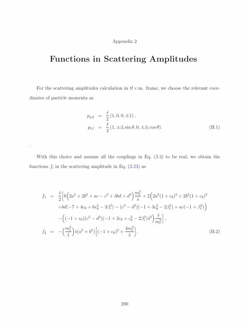
Appendix 2
Functions in Scattering Amplitudes
For the scattering amplitudes calculation in tt c.m. frame, we choose the relevant coor-
dinates of particle momenta as
pq,q =s
2(1, 0, 0,±1) ,
pt,t =s
2(1,±βt sin θ, 0,±βt cos θ). (B.1)
.
With this choice and assume all the couplings in Eq. (3.3) to be real, we obtain the
functions fi in the scattering amplitude in Eq. (3.23) as
f1 =s
2
[8(2a2 + 2b2 + ac− c2 + 3bd+ d2
)m2t
s+ 2
(2a2(1 + cθ)
2 + 2b2(1 + cθ)2
+bd(−7 + 4cθ + 6c2θ − 3β2t )− (c2 − d2)(−1 + 3c2θ − 2β2
t ) + ac(−1 + β2t ))
−((−1 + cθ)(c
2 − d2)(−1 + 2cθ + c2θ − 2β2t )s
2) s
m2t
],
f2 = −(m2
t
t
)s(a2 + b2)
[(−1 + cθ)
2 +4m2
t
s
]. (B.2)
200
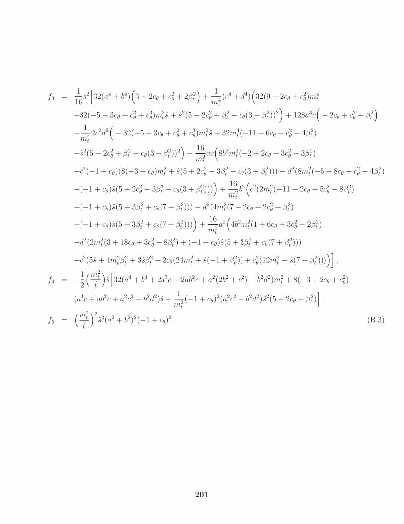
f3 =1
16s2[32(a4 + b4)
(3 + 2cθ + c2θ + 2β2
t
)+
1
m4t
(c4 + d4)(32(9− 2cθ + c2θ)m
4t
+32(−5 + 3cθ + c2θ + c3θ)m2t s+ s2(5− 2c2θ + β2
t − cθ(3 + β2t ))
2)+ 128a3c
(− 2cθ + c2θ + β2
t
)
− 1
m4t
2c2d2(− 32(−5 + 3cθ + c2θ + c3θ)m
2t s+ 32m4
t (−11 + 6cθ + c2θ − 4β2t )
−s2(5− 2c2θ + β2t − cθ(3 + β2
t ))2)+
16
m2t
ac(8b2m2
t (−2 + 2cθ + 3c2θ − 3β2t )
+c2(−1 + cθ)(8(−3 + cθ)m2t + s(5 + 2c2θ − 3β2
t − cθ(3 + β2t )))− d2(8m2
t (−5 + 8cθ + c2θ − 4β2t )
−(−1 + cθ)s(5 + 2c2θ − 3β2t − cθ(3 + β2
t ))))+
16
m2t
b2(c2(2m2
t (−11− 2cθ + 5c2θ − 8β2t )
−(−1 + cθ)s(5 + 3β2t + cθ(7 + β2
t )))− d2(4m2t (7− 2cθ + 2c2θ + β2
t )
+(−1 + cθ)s(5 + 3β2t + cθ(7 + β2
t ))))+
16
m2t
a2(4b2m2
t (1 + 6cθ + 3c2θ − 2β2t )
−d2(2m2t (3 + 18cθ + 3c2θ − 8β2
t ) + (−1 + cθ)s(5 + 3β2t + cθ(7 + β2
t )))
+c2(5s+ 4m2tβ
2t + 3sβ2
t − 2cθ(24m2t + s(−1 + β2
t )) + c2θ(12m2t − s(7 + β2
t ))))],
f4 = −1
2
(m2t
t
)s[32(a4 + b4 + 2a3c+ 2ab2c+ a2(2b2 + c2)− b2d2)m2
t + 8(−3 + 2cθ + c2θ)
(a3c+ ab2c+ a2c2 − b2d2)s+1
m2t
(−1 + cθ)2(a2c2 − b2d2)s2(5 + 2cθ + β2
t )],
f5 =(m2
t
t
)2
s2(a2 + b2)2(−1 + cθ)2. (B.3)
201
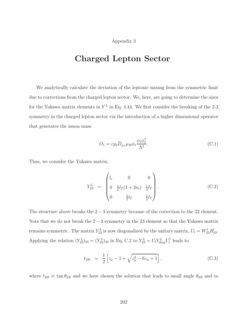
Appendix 3
Charged Lepton Sector
We analytically calculate the deviation of the leptonic mixing from the symmetric limit
due to corrections from the charged lepton sector. We, here, are going to determine the sizes
for the Yukawa matrix elements in Y L in Eq. 4.44. We first consider the breaking of the 2-3
symmetry in the charged lepton sector via the introduction of a higher dimensional operator
that generates the muon mass
O1 = cy2DµLµRφ1
φ1φ†1
Λ2. (C.1)
Thus, we consider the Yukawa matrix,
Y L23 =
le 0 0
0 12lT (1 + 2κl)
12lT
0 12lT
12lT
. (C.2)
The structure above breaks the 2− 3 symmetry because of the correction to the 22 element.
Note that we do not break the 2− 3 symmetry in the 23 element so that the Yukawa matrix
remains symmetric. The matrix Y L23 is now diagonalized by the unitary matrix, Ul =W l
23Rl23.
Applying the relation (Y L23)23 = (Y L
23)33 in Eq. C.2 to Y L23 = UlY
LdiagU
†l leads to
t23l =1
2
[zµ − 1 +
√z2µ − 6zµ + 1
], (C.3)
where t23l ≡ tan θ23l and we have chosen the solution that leads to small angle θ23l and to
202
small flavor symmetry breaking. Keeping terms up to first order in zµ we get
t23l ≈ −zµ. (C.4)
We further obtain for κl and lT in Eq. C.2,
κl = − tan 2θ23l ≈ 2zµ,
lT = (lτ − lµ) cos 2θ23l. (C.5)
Comparing the above equation with Eq. C.1, the size of the higher dimensional operator can
be estimated as
cv212Λ2
≈ 2zµ. (C.6)
Since v1 ≈ 250 GeV therefore the scale of Λ is in the TeV range.
To obtain a realistic charged lepton matrix, we take into account the mixing involving
the second and the third generations in the full Yukawa matrix
O2 = y′(DeLµR − DeLτR + DµL
eR − DτLeR)φ1φ1φ
†1
Λ2. (C.7)
Thus, the full mixing matrix will be give by
Y L =
l11 l12 −l12l12
12lT (1 + 2κl)
12lT
−l12 12lT
12lT
. (C.8)
We will assume that the Yukawa matrix Y L is now diagonalized by the unitary matrix Ul
given by
Ul = W l23R
l23R
l13R
l12. (C.9)
203
From the Yukawa matrix (C.8), one can find the two relations
Y12 = −Y13,
Y22 =1
2(Y23 + Y33)(1 + 2κl). (C.10)
Applying the above two relations to
Y L = UlYLdiagU
†l (C.11)
using Eq. C.9, one can obtain the solutions
s12l ≈ ±c23l
√zµ − 2κl + (−3 + 3zµ − 2κl)c23ls23l + 2zµκlc23ls23l
zµ − z2µ(3 + 2κl)c23ls23l,
s13l ≈ ±√zµc12ls23l
√zµ − 2κl + (−3 + 3zµ − 2κl)c23ls23l + 2zµκlc23ls23l
1− zµ(3 + 2κl)c23ls23l. (C.12)
By comparing Eqs. (C.8, C.11), one can get the matrix element l12 after substituting
Eqs. (C.4, C.5, C.12) up to the first order in zµ
l12 ≈√zµ2(le − lµ). (C.13)
The leptonic mixing matrix is now given by
UPMNS = U †ℓUν , (C.14)
where Uℓ =W l23R
l23R
l13R
l12 and Uν = W ν
12.
204
Appendix 4
Hadronic form factors
The expressions for the vector and axial-vector hadronic currents in Eq. D.9 are
〈p(p′)|Vµ|n(p)〉 = up(p′)[γµF
V1 +
i
2Mσµνq
νF V2 +
qµMFS
]un(p),
−〈p(p′)|Aµ|n(p)〉 = up(p′)[γµFA +
i
2Mσµνq
νFT +qµMFP
]γ5un(p). (D.1)
Here q = p′ − p and the form factors Fi are functions of t = q2. The parametrizations of the
axial-vector and pseudoscalar form factors are [291]
FA(t) = FA(0)(1− t
M2A
)−2
,
FP (t) =2M2FA(0)
m2π − t
, (D.2)
where FA(0) = −1.2695 is the axial coupling [168], mπ is the charged pion mass, and MA =
1.35 GeV is the axial-vector mass [305]. The expression for FP (t) can be shown to be true
at low energy, where the predictions of chiral perturbation theory are valid [306]. We have
assumed the relation to hold at high t also. Note that FA(0) is sometimes replaced by FA(t),
which gives similar results for FP (t) at low t but very different results at high t.
The Dirac and Pauli form factors F V1,2 are
F V1 (t) =
GE(t)− xtGM(t)
1− xt, F V
2 (t) =GM(t)−GE(t)
1− xt, (D.3)
205
where xt = t/4M2 and
GM = GpM −Gn
M , GE = GpE −Gn
E . (D.4)
Here Gp,nE and Gp,n
M are the electric and magnetic form factors of the proton and neutron,
respectively. The simplest parametrizations of these form factors are given by the dipole
approximation
GpE ≈ GD, G
nE ≈ 0, Gp
M ≈ µpGD, GnM ≈ µnGD , (D.5)
where GD = (1−t/M2V )
−2,MV = 0.843 GeV is the vector mass, and µp(µn) is the anomalous
magnetic moment of the proton (neutron) [307].
In the presence of the charged Higgs, applying the equation of motion to the hadronic
matrix elements for the scalar and pseudoscalar currents for the process ντ + n → τ− + p
gives
〈p(p′)|u(guidjS − g
uidjP γ5)d|n(p)〉 = Vud p(p4)
(guidjS GS + g
uidjP GPγ5
)n(p2), (D.6)
or
〈p(p′)|ud|n(p)〉 = p(p4)GSn(p2),
−〈p(p′))|uγ5d|n(p)〉 = p(p4)GPγ5n(p2) , (D.7)
where
GS(t) = rNFV1 (t), with rN =
Mn −Mp
(md −mu)∼ O(1),
GP (t) =M [FA(t) + 2xtFP (t)]
mq, (D.8)
206
with mq = (mu +md)/2. In the W ′ model, the current has both V ±A structures. One has
to calculate the matrix element,
〈p(p′)|J+µ |n(p)〉 = Vud 〈p(p′)|u
(gudL γµ(1− γ5) + gudR γµ(1 + γ5)
)d|n(p)〉. (D.9)
Kinematic details
The Mandelstam variables in terms of Eν and the lepton energy El are
s = M2 + 2MEν , t = 2M(El − Eν),
s− u = 4MEν + t−m2l . (D.10)
Then t and El lie in the intervals
m2l − 2Ecm
ν (Ecml + pcml ) ≤ t ≤ m2
l − 2Ecmν (Ecm
l − pcml ) , (D.11)
Eν +m2
l − 2Ecmν (Ecm
l + pcml )
2M≤ El ≤ Eν +
m2l − 2Ecm
ν (Ecml − pcml )
2M, (D.12)
where the energy and momentum of the lepton and the neutrino in the center of mass (cm)
system are
Ecmν =
(s−M2)
2√s
, pcml =√
(Ecml )2 −m2
l ,
Ecml =
(s−M2 +m2l )
2√s
. (D.13)
The threshold neutrino energy to create the charged lepton partner is given by
Ethνl
=(ml +Mp)
2 −M2n
2Mn, (D.14)
207
where ml, Mp, Mn are the masses of the charged lepton, proton, and neutron, respectively.
In our case, the threshold energy of the tau neutrino is Ethντ = 3.45 GeV.
The differential cross section in the laboratory frame is given by
dσtot(νl)
dt=
|M|264πE2
νM2. (D.15)
The expressions for the coefficients fSM (f = A,B,C) in the SM differential cross section
[see Eq.(7.20)] are
ASM = 4(xt − xl)[(F V
1 )2(1 + xl + xt) + (FA)2(−1 + xl + xt) + (F V
2 )2(xl + x2t + xt)
+4F 2Pxlxt + 2F V
1 FV2 (xl + 2xt) + 4FAFPxl
],
BSM = 4xtFA(FV1 + F V
2 ) ,
CSM =(F V
1 )2 + F 2A − xt(F
V2 )2
4, (D.16)
where xl = m2l /4M
2.
The expressions for the quantities AI,PH andBI
H in the differential cross section in Eq. (7.33)
are
AIH = 2
√xl(xt − xl)g
udP (glνlS − glνlP )GP (FA + 2FPxt) ,
BIH =
1
2
√xlg
udS (glνlS − glνlP )GS(F
V1 + F V
2 xt) ,
APH = 2(xt − xl)(|glνlS |2 + |glνlP |2)(|gudP |2G2
Pxt + |gudS |2G2S(xt − 1)) . (D.17)
For the 2HDM II model couplings, gS,P are given in Eq. (7.46). Note that the interference
208
terms AIH and BI
H vanish in this model.
The expressions for the quantities f ′ (f = A,B,C) in the differential cross section in Eq.
(7.41) are
A′ = 4(xt − xl)[(1 + rρW ′)
2((F V
1 )2(1 + xl + xt) + 2F V1 F
V2 (xl + 2xt) + (F V
2 )2(xl + x2t + xt))
+(1 + rπW ′)2((FA)
2(−1 + xl + xt) + 4FAFPxl + 4F 2Pxlxt
)],
B′ = 4Re[(1 + rρW ′)(1 + rπ∗W ′)]xtFA(FV1 + F V
2 ) ,
C ′ =1
4
[(1 + rρW ′)
2((F V1 )2 − xt(F
V2 )2) + (1 + rπW ′)2F 2
A
]. (D.18)
In the absence of W ′ contributions, the f ′’s reduce to the respective SM results in Eq. D.16.
209
Bibliography
[1] K. Abe et al. [T2K Collaboration], Phys. Rev. Lett. 107, 041801 (2011) [arXiv:1106.2822
[hep-ex]]. 2, 12, 87
[2] L. Whitehead [MINOS Collaboration], “Recent results from MINOS”, Joint
Experimental-Theoretical Seminar (24 June 2011, Fermilab, USA). Websites: the-
ory.fnal.gov/jetp, http://www-numi.fnal.gov/pr-plots/ 2, 12
[3] P. Adamson et al. [MINOS Collaboration], “Improved search for muon-neutrino to
electron-neutrino oscillations in MINOS,” arXiv:1108.0015 [hep-ex]. 2
[4] L. Wolfenstein, Phys. Rev. D 17, 2369 (1978); L. Wolfenstein, Phys. Rev. D 20, 2634
(1979); S. P. Mikheev and A. Y. Smirnov, Sov. J. Nucl. Phys. 42, 913 (1985) [Yad. Fiz.
42, 1441 (1985)]; S. P. Mikheev and A. Y. Smirnov, Nuovo Cim. C 9, 17 (1986). V. D.
Barger, K. Whisnant, S. Pakvasa and R. J. N. Phillips, Phys. Rev. D 22, 2718 (1980).
2
[5] F. Englert and R. Brout, Phys. Rev. Lett. 13, 321 (1964). 3
[6] P. W. Higgs, Phys. Rev. Lett. 13, 508 (1964).
[7] G. S. Guralnik, C. R. Hagen and T. W. B. Kibble, Phys. Rev. Lett. 13, 585 (1964). 3
3
210
BIBLIOGRAPHY
[8] John F. Gunion, Howard E. Haber, Gordon Kane, and Sally Dawson. Book title “The
Higgs Hunter’s Guide”. ISBN: 0-7382-0305-X. 6
[9] [CMS Collaboration], CMS-PAS-HIG-12-020. 8
[10] [ATLAS Collaboration], ATLAS-CONF-2012-093. 8
[11] S. Chang, R. Dermisek, J. F. Gunion and N. Weiner, Ann. Rev. Nucl. Part. Sci. 58, 75
(2008) [arXiv:0801.4554 [hep-ph]]. 8, 42
[12] B. Aubert et al. [BABAR Collaboration], Phys. Rev. Lett. 101, 071801 (2008) [Erratum-
ibid. 102, 029901 (2009)], hep-ex/0807.1086v4. 8, 43
[13] B. Aubert et al. [BABAR Collaboration], hep-ex/0903.1124. 9, 43, 50
[14] S.W. Herb et al., Phys. Rev. Lett. 39, 252 (1977); W.R. Innes et al., Phys. Rev. Lett.
39, 1240 (1977) [Erratum-ibid. 39, 1640(E) (1977)]. 9
[15] A. H. Mahmood et al. [CLEO Collaboration], hep-ex/0207057, M. Artuso et al. [CLEO
Collaboration], Phys. Rev. Lett. 94, 032001 (2005), hep-ex/0411068. 9
[16] A. Heister et al. [ALEPH Collaboration], Phys. Lett. B 530, 56 (2002), hep-ex/0202011,
M. Levtchenko [L3 Collaboration], Nucl. Phys. Proc. Suppl. 126, 260 (2004). A. Sokolov,
Nucl. Phys. Proc. Suppl. 126, 266 (2004). J. Abdallah [DELPHI Collaboration], Phys.
Lett. B 634, 340 (2006), hep-ex/0601042. N. Brambilla et al. [Quarkonium Working
Group], arXiv:hep-ph/0412158. 9, 42
[17] F. Maltoni and A. D. Polosa, Phys. Rev. D 70, 054014 (2004) [arXiv:hep-ph/0405082].
9, 42
[18] T. W. Chiu, T. H. Hsieh, C. H. Huang and K. Ogawa [TWQCD Collaboration], Phys.
Lett. B 651, 171 (2007) [arXiv:0705.2797 [hep-lat]], A. Gray, I. Allison, C. T. H. Davies,
E. Dalgic, G. P. Lepage, J. Shigemitsu and M. Wingate, Phys. Rev. D 72, 094507
211
BIBLIOGRAPHY
(2005) [arXiv:hep-lat/0507013], T. Burch and C. Ehmann, Nucl. Phys. A 797, 33 (2007)
[arXiv:hep-lat/0701001]. 9
[19] A. Penin, arXiv:0905.4296v1 [hep-ph]. 9
[20] B. A. Kniehl, A. A. Penin, A. Pineda, V. A. Smirnov and M. Steinhauser, Phys. Rev.
Lett. 92, 242001 (2004) [Erratum-ibid. 104, 199901 (2010)] [arXiv:hep-ph/0312086]. 9
[21] B. Aubert et al. [BABAR Collaboration], Phys. Rev. Lett. 103, 181801 (2009)
[arXiv:0906.2219 [hep-ex]]. 9, 41
[22] T. Aaltonen et al. [CDF Collaboration], arXiv:1101.0034 [hep-ex]. xv, 10, 66
[23] J. H. Kuhn and G. Rodrigo, Phys.Rev.Lett. 81 (1998) 49, [hep-ph/9802268]. 10
[24] J. H. Kuhn and G. Rodrigo, Phys.Rev. D59 (1999) 054017, [ hep-ph/9807420]. 10
[25] M. Bowen, S. Ellis, and D. Rainwater, Phys.Rev.D73 (2006) 014008, [ hep-ph/0509267].
10
[26] L. G. Almeida, G. F. Sterman, and W. Vogelsang, Phys.Rev. D78 (2008) 014008,
[arXiv:0805.1885 [hep-ph]]. 10
[27] D0 Collaboration, V. Abazov et. al., Phys.Rev.Lett. 100 (2008) 142002, [
arXiv:0712.0851 [hep-ex]]. 10
[28] T. Aaltonen et al. [CDF Collaboration], Conf. Note 9913 (2009); 10
[29] U. Langenfeld, S. Moch, and P. Uwer , Phys. Rev. D. 80, 054009 (2009).
[arXiv:0906.5273[hep-ph]].
[30] M. Cacciari et al. , JHEP 09, 127 (2008). [arXiv:0804.2800[hep-ph]]. 10
10
212
BIBLIOGRAPHY
[31] N. Kidonakis and R. Vogt , Phys. Rev. D. 78, 074005 (2008). [arXiv:0805.3844 [hep-ph]].
10
[32] V. Ahrens, A. Ferroglia, M. Neubert, B. D. Pecjak and L. Li , JHEP 09, 097 (2010).
[arXiv:1003.5827[hep-ph]]. 10
[33] L. Sehgal and M. Wanninger, B200 (1988) 211. J. Bagger, C. Schmidt, and S. King,
Phys.Rev.D37 (1988) 1188. P. Ferrario and G. Rodrigo, Phys.Rev. D80 (2009) 051701,[
arXiv:0906.5541[hep-ph]]. P. H. Frampton, J. Shu, and K. Wang, Phys. Lett. B683
(2010) 294, [ arXiv:0911.2955 [hep-ph]]. R. Chivukula, E. H. Simmons, and C.-P. Yuan,
Phys.Rev. D82 (2010) 094009, [ arXiv:1007.0260 [hep-ph]]. A. Djouadi, G. Moreau,
F. Richard, and R. K. Singh, Phys.Rev. D82 (2010) 071702, [arXiv:0906.0604 [hep-
ph]]. M. Bauer, F. Goertz, U. Haisch, T. Pfoh, and S. Westhoff, JHEP 1011
(2010) 039, [arXiv:1008.0742 [hep-ph]]. E. Alvarez, L. Da Rold, and A. Szynkman,
arXiv:1011.6557 [hep-ph]. C.-H. Chen, G. Cvetic, and C. Kim, Phys.Lett. B694 (2011)
393, [ arXiv:1009.4165 [hep-ph] ]. C. Delaunay, O. Gedalia, S. J. Lee, G. Perez, E. Pon-
ton, arXiv:1101.2902 [hep-ph]. Y. Bai, J. L. Hewett, J. Kaplan, T. G. Rizzo, JHEP
1103 (2011) 003, [arXiv:1101.5203 [hep-ph]]. A. R. Zerwekh, arXiv:1103.0956 [hep-ph].
E. R. Barreto, Y. A. Coutinho, J. S. Borges, arXiv:1103.1266 [hep-ph]. A. Djouadi,
G. Moreau, F. Richard, arXiv:1105.3158 [hep-ph]. R. Barcelo, A. Carmona, M. Masip,
J. Santiago, arXiv:1105.3333 [hep-ph] S. Westhoff, arXiv:1105.4624[hep-ph]. U. Haisch,
S. Westhoff, arXiv:1106.0529[hep-ph]. E. Gabrielli, M. Raidal, arXiv:1106.4553 [hep-
ph]. 10
[34] S. Jung, H. Murayama, A. Pierce, and J. D. Wells, Phys. Rev. D81 (2010) 015004,
[ arXiv:0907.4112 [hep-ph]]. K. Cheung, W.-Y. Keung, and T.-C. Yuan, Phys.Lett.
B682 (2009) 287, [arXiv:0908.2589 [hep-ph]]. J. Shu, T. M. P. Tait, and K. Wang,
Phys. Rev. D81 (2010) 034012, [ arXiv:0911.3237 [hep-ph]]. I. Dorsner, S. Fajfer,
213
BIBLIOGRAPHY
J. F. Kamenik, and N. Kosnik, Phys.Rev. D81 (2010) 055009, [arXiv:0912.0972 [hep-
ph] ]. A. Arhrib, R. Benbrik, and C.-H. Chen, Phys. Rev. D82 (2010) 034034,
[arXiv:0911.4875 [hep-ph]]. V. Barger, W.-Y. Keung, and C.-T. Yu, Phys. Rev.
D81 (2010) 113009, [arXiv:1002.1048 [hep-ph]]. S. K. Gupta, G. Valencia, Phys.
Rev. D82, 035017 (2010). [arXiv:1005.4578 [hep-ph]]. B. Xiao, Y.-k. Wang, and S.-
h. Zhu, Phys.Rev. D82 (2010) 034026, [arXiv:1006.2510 [hep-ph] ]. S. K. Gupta,
arXiv:1011.4960 [hep-ph]. K. Cheung and T.-C. Yuan, arXiv:1101.1445 [hep-ph]. J. Cao,
L. Wang, L. Wu, J. M. Yang, [arXiv:1101.4456 [hep-ph]. E. L. Berger, Q. -H. Cao, C. -
R. Chen, C. S. Li, H. Zhang, arXiv:1101.5625 [hep-ph]. V. Barger, W. -Y. Keung,
C. -T. Yu, arXiv:1102.0279 [hep-ph]. B. Grinstein, A. L. Kagan, M. Trott, J. Zupan,
arXiv:1102.3374 [hep-ph]. K. M. Patel, P. Sharma, arXiv:1102.4736 [hep-ph]. S. Jung,
A. Pierce, J. D. Wells, arXiv:1103.4835 [hep-ph]. M. R. Buckley, D. Hooper, J. .Kopp,
E. .Neil, arXiv:1103.6035[hep-ph]. J. Shu, K. Wang, G. Zhu, arXiv:1104.0083 [hep-ph].
A. Rajaraman, Z. Surujon, T. M. P. Tait, arXiv:1104.0947 [hep-ph]. J. A. Aguilar-
Saavedra, M. Perez-Victoria, arXiv:1104.1385 [hep-ph]. C. Degrande, J. M. Gerard,
C. Grojean, F. Maltoni, G. Servant, arXiv:1104.1798 [hep-ph]. X. P. Wang,Y. K. Wang,
B. Xiao, J. Xu, S. h. Zhu, arXiv:1104.1917 [hep-ph]. A. E. Nelson, T. Okui, T. S. Roy,
arXiv:1104.2030 [hep-ph]. S. Jung, A. Pierce, J. D. Wells, arXiv:1104.3139 [hep-ph].
D. W. Jung, P. Ko, S. J. Lee, arXiv:1104.4443 [hep-ph]. K. S. Babu, M. Frank, S. K. Rai,
arXiv:1104.4782 [hep-ph]. J. A. Aguilar-Saavedra, M. Perez-Victoria, arXiv:1105.4606
[hep-ph]. 10, 65
[35] K. Kodama et al. (DONUT), Phys. Lett. B504 (2001), 218, hep-ex/0012035 11
[36] Super-Kamiokande, Y. Fukuda et al., Evidence for oscillation of atmospheric neutrinos,
Phys. Rev. Lett. 81 (1998), 1562, hep-ex/9807003. Super-Kamiokande, Y. Ashie et al.,
Evidence for an oscillatory signature in atmospheric neutrino oscillation, Phys. Rev.
Lett. 93 (2004), 101801, hep-ex/0404034. 11
214
BIBLIOGRAPHY
[37] Super-Kamiokande, J. P. Cravens et al., Solar neutrino measurements in Super-
Kamiokande-II, Phys. Rev. D78 (2008), 032002, 0803.4312. B. T. Cleveland et al.,
Measurement of the solar electron neutrino flux with the Homestake chlorine detec-
tor, Astrophys. J. 496 (1998), 505. SAGE, J. N. Abdurashitov et al., Measurement of
the solar neutrino capture rate by the Russian-American gallium solar neutrino exper-
iment during one half of the 22-year cycle of solar activity, J. Exp. Theor. Phys. 95
(2002), 181, astro-ph/0204245. GALLEX, W. Hampel et al., GALLEX solar neutrino
observations: Results for GALLEX IV, Phys. Lett. B447 (1999), 127. GNO, M. Alt-
mann et al., GNO solar neutrino observations: Results for GNO I, Phys. Lett. B490
(2000), 16, hep-ex/0006034. 11
[38] SNO, Q. R. Ahmad et al., Direct evidence for neutrino flavor transformation from
neutral-current interactions in the Sudbury Neutrino Observatory, Phys. Rev. Lett. 89
(2002), 011301, nucl-ex/0204008. 11
[39] Super-Kamiokande, Y. Ashie et al., A measurement of atmospheric neutrino oscillation
parameters by Super-Kamiokande I, Phys. Rev. D71 (2005), 112005, hep-ex/0501064.
12
[40] KamLAND, K. Eguchi et al., First results from KamLAND: Evidence for reactor anti-
neutrino disappearance, Phys. Rev. Lett. 90 (2003), 021802, hep-ex/0212021. The Kam-
LAND Collaboration, Precision measurement of neutrino oscillation parameters with
KamLAND, (2008), arXiv:0801.4589 [hep-ex]. 12
[41] CHOOZ, M. Apollonio et al., Search for neutrino oscillations on a long baseline at the
CHOOZ nuclear power station, Eur. Phys. J. C27 (2003), 331, hep-ex/0301017. 12
[42] K2K, M. H. Ahn et al., Indications of neutrino oscillation in a 250-km long- baseline
experiment, Phys. Rev. Lett. 90 (2003), 041801, hep-ex/0212007. K2K,M. H. Ahn et al.,
215
BIBLIOGRAPHY
Measurement of neutrino oscillation by the K2K experiment, Phys. Rev. D74 (2006),
072003, hep-ex/0606032. 12
[43] MINOS, D. G. Michael et al., Observation of muon neutrino disappearance with the
MINOS detectors and the NuMI neutrino beam, Phys. Rev. Lett. 97 (2006), 191801, hep-
ex/0607088. MINOS, P. Adamson et al., Measurement of neutrino oscillations with the
MINOS detectors in the NuMI beam, Phys. Rev. Lett. 101 (2008), 131802, 0806.2237.
12
[44] Y. Abe et al. [DOUBLE-CHOOZ Collaboration], Phys. Rev. Lett. 108, 131801 (2012)
[arXiv:1112.6353 [hep-ex]]. 12
[45] F. P. An et al. [DAYA-BAY Collaboration], Phys. Rev. Lett. 108, 171803 (2012)
[arXiv:1203.1669 [hep-ex]]. 12
[46] J. K. Ahn et al. [RENO Collaboration], Phys. Rev. Lett. 108, 191802 (2012)
[arXiv:1204.0626 [hep-ex]]. 12
[47] D. V. Forero, M. Tortola and J. W. F. Valle, arXiv:1205.4018 [hep-ph]. xviii, xx, xxii,
xxiii, 12, 105, 147, 158, 162, 169, 170
[48] D. Marzocca, S. T. Petcov, A. Romanino, M. Spinrath, [arXiv:1108.0614 [hep-ph]].
Y. H. Ahn, H. -Y. Cheng, S. Oh, [arXiv:1107.4549 [hep-ph]]. R. d. A. Toorop,
F. Feruglio, C. Hagedorn, [arXiv:1107.3486 [hep-ph]]. P. S. Bhupal Dev, R. N. Mo-
hapatra, M. Severson, [arXiv:1107.2378 [hep-ph]]. S. Dev, S. Gupta, R. R. Gau-
tam, [arXiv:1107.1125 [hep-ph]]. D. Meloni, [arXiv:1107.0221 [hep-ph]]. N. Haba,
R. Takahashi, Phys. Lett. B702, 388-393 (2011). [arXiv:1106.5926 [hep-ph]]. S. Zhou,
[arXiv:1106.4808 [hep-ph]]. X. -G. He, A. Zee, [arXiv:1106.4359 [hep-ph]]. Y. -j. Zheng,
B. -Q. Ma, [arXiv:1106.4040 [hep-ph]]. H. Ishimori, T. Kobayashi, [arXiv:1106.3604
[hep-ph]]. M. -C. Chen, K. T. Mahanthappa, A. Meroni, S. T. Petcov, [arXiv:1109.0731
216
BIBLIOGRAPHY
[hep-ph]]. S. Davidson, M. Elmer, [arXiv:1108.0548 [hep-ph]]. J. Heeck, W. Rodejohann,
Phys. Rev. D84, 075007 (2011). [arXiv:1107.5238 [hep-ph]]. S. Antusch, V. Maurer,
[arXiv:1107.3728 [hep-ph]]. X. -G. He, S. K. Majee, [arXiv:1111.2293 [hep-ph]]. N. Haba,
T. Horita, K. Kaneta, Y. Mimura, [arXiv:1110.2252 [hep-ph]]. A. Aranda, C. Bonilla,
A. D. Rojas, [arXiv:1110.1182 [hep-ph]]. 13, 18, 70
[49] S. Kumar, [arXiv:1108.2137 [hep-ph]]. H. Fritzsch, Z. -z. Xing, S. Zhou, [arXiv:1108.4534
[hep-ph]]. S. Antusch, S. F. King, C. Luhn, M. Spinrath, [arXiv:1108.4278 [hep-ph]].
M. Huang, D. Liu, J. -C. Peng, S. D. Reitzner, W. -C. Tsai, [arXiv:1108.3906 [hep-
ph]]. T. Araki, C. -Q. Geng, [arXiv:1108.3175 [hep-ph]]. Riazuddin, [arXiv:1108.1469
[hep-ph]]. T. Schwetz, M. Tortola, J. W. F. Valle, [arXiv:1108.1376 [hep-ph]]. S. -
F. Ge, D. A. Dicus, W. W. Repko, [arXiv:1108.0964 [hep-ph]]. G. J. Mathews, T. Ka-
jino, W. Aoki, W. Fujiya, [arXiv:1108.0725 [astro-ph.HE]]. S. F. King, C. Luhn,
[arXiv:1107.5332 [hep-ph]]. M. -C. Chen, K. T. Mahanthappa, [arXiv:1107.3856 [hep-
ph]]. W. Rodejohann, H. Zhang, S. Zhou, [arXiv:1107.3970 [hep-ph]]. X. Chu, M. Dhen,
T. Hambye, [arXiv:1107.1589 [hep-ph]]. H. Zhang, S. Zhou, [arXiv:1107.1097 [hep-
ph]]. W. Chao, Y. -j. Zheng, [arXiv:1107.0738 [hep-ph]]. S. Morisi, K. M. Patel,
E. Peinado, [arXiv:1107.0696 [hep-ph]]. G. L. Fogli, E. Lisi, A. Marrone, A. Palazzo,
A. M. Rotunno, [arXiv:1106.6028 [hep-ph]]. T. Araki, Phys. Rev. D84, 037301 (2011).
[arXiv:1106.5211 [hep-ph]]. A. B. Balantekin, [arXiv:1106.5021 [hep-ph]]. S. F. King,
[arXiv:1106.4239 [hep-ph]]. E. Ma, D. Wegman, Phys. Rev. Lett. 107, 061803 (2011).
[arXiv:1106.4269 [hep-ph]]. J. -M. Chen, B. Wang, X. -Q. Li, [arXiv:1106.3133 [hep-
ph]]. Z. -z. Xing, [arXiv:1106.3244 [hep-ph]]. N. Qin, B. Q. Ma, Phys. Lett. B702,
143-149 (2011). [arXiv:1106.3284 [hep-ph]]. J. Barry, W. Rodejohann, H. Zhang,
JHEP 1107, 091 (2011). [arXiv:1105.3911 [hep-ph]]. Q. -H. Cao, S. Khalil, E. Ma,
H. Okada, [arXiv:1108.0570 [hep-ph]]. S. Antusch, P. Di Bari, D. A. Jones, S. F. King,
[arXiv:1107.6002 [hep-ph]]. M. Blennow, E. Fernandez-Martinez, Phys. Lett. B704,
217
BIBLIOGRAPHY
223 (2011). [arXiv:1107.3992 [hep-ph]]. A. Adulpravitchai, R. Takahashi, JHEP
1109, 127 (2011). [arXiv:1107.3829 [hep-ph]]. S. Dev, S. Gupta, R. R. Gautam,
L. Singh, [arXiv:1111.1300 [hep-ph]]. Y. -L. Zhou, [arXiv:1110.5023 [hep-ph]]. D. Mel-
oni, [arXiv:1110.5210 [hep-ph]]. P. Coloma, E. Fernandez-Martinez, [arXiv:1110.4583
[hep-ph]]. G. -J. Ding, L. L. Everett, A. J. Stuart, [arXiv:1110.1688 [hep-ph]]. G. Bhat-
tacharyya, H. Pas, D. Pidt, [arXiv:1109.6183 [hep-ph]]. C. Hartmann, [arXiv:1109.5143
[hep-ph]]. 13, 18
[50] V. M. Lobashev et al., Direct search for mass of neutrino and anomaly in the tritium
beta-spectrum, Phys. Lett. B460 (1999), 227. C. Kraus et al., Final results from phase
II of the Mainz neutrino mass search in tritium beta decay, Eur. Phys. J. C40 (2005),
447, hep-ex/0412056. 13
[51] G. L. Fogli et al., Observables sensitive to absolute neutrino masses (Addendum), Phys.
Rev. D78 (2008), 033010, 0805.2517. 13
[52] H. V. Klapdor-Kleingrothaus et al., Latest results from the Heidelberg- Moscow double-
beta- decay experiment, Eur. Phys. J. A12 (2001), 147, hep-ph/0103062. 13
[53] S. Davidson, C. Pena-Garay, N. Rius, and A. Santamaria, Present and future bounds
on non-standard neutrino interactions, JHEP 03 (2003), 011, hep-ph/0302093. M. C.
Gonzalez-Garcia and M. Maltoni, Phenomenology with massive neutrinos, Phys. Rept.
460 (2008), 1, 0704.1800. M. Maltoni, New interactions: past and future experiments,
J. Phys. Conf. Ser. 136 (2008), 022024, 0810.3517. 13
[54] M. C. Gonzalez-Garcia and M. Maltoni, Status of oscillation plus decay of atmospheric
and long-baseline neutrinos, Phys. Lett. B663 (2008), 405, 0802.3699. 13
[55] Y. Farzan, T. Schwetz, and A. Y. Smirnov, Reconciling results of LSND, Mini- BooNE
and other experiments with soft decoherence, JHEP 07 (2008), 067, 0805.2098. 13
218
BIBLIOGRAPHY
[56] M. Maltoni and T. Schwetz, Sterile neutrino oscillations after first MiniBooNE results,
Phys. Rev. D76 (2007), 093005, 0705.0107. 13
[57] J. N. Bahcall, arXiv:physics/0406040; R. N. Mohapatra et al., arXiv:hep-ph/0510213;
R. N. Mohapatra and A. Y. Smirnov, Ann. Rev. Nucl. Part. Sci. 56 (2006) 569
[arXiv:hep-ph/0603118]; S. F. King, Rept. Prog. Phys. 67 (2004) 107 [arXiv:hep-
ph/0310204]; G. Altarelli and F. Feruglio, New J. Phys. 6 (2004) 106 [arXiv:hep-
ph/0405048]. 13
[58] Z. Maki, M. Nakagawa and S. Sakata, Prog. Theo. Phys. 28 (1962) 247; B. W. Lee,
S. Pakvasa, R. E. Shrock and H. Sugawara, Phys. Rev. Lett. 38 (1977) 937 [Erratum-
ibid. 38 (1977) 1230]. W.-M. Yao et al. [Particle Data Group Collaboration], 14
[59] A. Upadhyay and M. Batra, arXiv:1112.0445 [hep-ph]. 15, 138
[60] H. Fritzsch and Z. Z. Xing, Phys. Lett. B 372, 265 (1996); Phys. Lett. B 440, 313
(1998); Phys. Rev. D 61,073016 (2000). 17
[61] Z. Z. Xing, arXiv:1106.3244[hep-ph]. 17
[62] F. Vissani, hep-ph/9708483; V.D. Barger, S.Pakvasa, T.J. Weiler, and K. Whisnant,
Phys. Lett. B437, 107 (1998); A.J. Baltz, A.S. Goldhaber, and M. Goldhaber, Phys.
Rev. Lett. 81, 5730 (1998); I. Stancu and D.V. Ahluwalia, Phys. Lett. B460, 431 (1999);
H. Georgi and S.L. Glashow, Phy. Rev. D61, 097301 (2000); N. Li and B.-Q. Ma, Phys.
Lett. B 600, 248 (2004) [arXiv:hep-ph/0408235]. 17
[63] V. Barger, S. Pakvasa, T. Weiler and K. Whisnant, Phys. Lett. B 437, 107 (1998); N. Li
and B. Q. Ma, Phys. Lett. B 600, 248 (2004) [arXiv:hep-ph/0408235]. I. Stancu and
D. V. Ahluwalia, Phys. Lett. B 460, 431 (1999) [arXiv:hep-ph/9903408]. 17
[64] P.F. Harrison, D.H. Perkins, and W.G. Scott, Phys. Lett. B458, 79 (1999); Phys.
Lett. B530, 167 (2002); Z.Z. Xing, Phys. Lett. B533, 85 (2002); P.F. Harrison and
219
BIBLIOGRAPHY
W.G. Scott, Phys. Lett. B535, 163 (2002); Phys. Lett. B557, 76 (2003); X.-G. He and
A. Zee, Phys. Lett. B560, 87 (2003); See also L. Wolfenstein, Phys. Rev. D18, 958
(1978); Y. Yamanaka, H. Sugawara, and S. Pakvasa, Phys. Rev. D25, 1895 (1982);
D29, 2135(E) (1984); N. Li and B.-Q. Ma, Phys. Rev. D 71, 017302 (2005) [arXiv:hep-
ph/0412126]. 17
[65] For a list of flavor symmetries and references see C. S. Lam, arXiv:0809.1185 [hep-ph].
17
[66] For work related to TBM see also, for an incomplete list: P. H. Frampton, S. T. Pet-
cov and W. Rodejohann, Nucl. Phys. B 687 (2004) 31 [arXiv:hep-ph/0401206];
A. Dighe, S. Goswami and W. Rodejohann, Phys. Rev. D 75 (2007) 073023 [arXiv:hep-
ph/0612328]; F. Plentinger and W. Rodejohann, Phys. Lett. B 625 (2005) 264
[arXiv:hep-ph/0507143]; R. N. Mohapatra and W. Rodejohann, Phys. Rev. D 72 (2005)
053001 [arXiv:hep-ph/0507312]; K. A. Hochmuth, S. T. Petcov and W. Rodejohann,
arXiv:0706.2975 [hep-ph]. G. Altarelli, F. Feruglio and Y. Lin, Nucl. Phys. B 775
(2007) 31 [arXiv:hep-ph/0610165]; G. Altarelli and F. Feruglio, Nucl. Phys. B 741
(2006) 215 [arXiv:hep-ph/0512103]; G. Altarelli and F. Feruglio, Nucl. Phys. B 720
(2005) 64 [arXiv:hep-ph/0504165]; F. Feruglio, C. Hagedorn, Y. Lin and L. Merlo,
Nucl. Phys. B 775 (2007) 120 [arXiv:hep-ph/0702194]. E. Ma, arXiv:0709.0507 [hep-ph];
E. Ma, arXiv:hep-ph/0701016; E. Ma, Mod. Phys. Lett. A 22 (2007) 101 [arXiv:hep-
ph/0610342]; E. Ma, Mod. Phys. Lett. A 21 (2006) 2931 [arXiv:hep-ph/0607190]; E. Ma,
Mod. Phys. Lett. A 21 (2006) 1917 [arXiv:hep-ph/0607056]; E. Ma, H. Sawanaka
and M. Tanimoto, Phys. Lett. B 641 (2006) 301 [arXiv:hep-ph/0606103]; E. Ma,
Phys. Rev. D 73 (2006) 057304; B. Adhikary, B. Brahmachari, A. Ghosal, E. Ma
and M. K. Parida, Phys. Lett. B 638 (2006) 345 [arXiv:hep-ph/0603059]; E. Ma,
Mod. Phys. Lett. A 20 (2005) 2601 [arXiv:hep-ph/0508099]; E. Ma, Phys. Rev. D
72 (2005) 037301 [arXiv:hep-ph/0505209]; S. L. Chen, M. Frigerio and E. Ma, Nucl.
220
BIBLIOGRAPHY
Phys. B 724 (2005) 423 [arXiv:hep-ph/0504181]; E. Ma, Phys. Rev. D 70 (2004) 031901
[arXiv:hep-ph/0404199]. I. de Medeiros Varzielas and G. G. Ross, Nucl. Phys. B 733
(2006) 31 [arXiv:hep-ph/0507176]; I. de Medeiros Varzielas, S. F. King and G. G. Ross,
Phys. Lett. B 644 (2007) 153 [arXiv:hep-ph/0512313]; I. de Medeiros Varzielas,
S. F. King and G. G. Ross, Phys. Lett. B 648 (2007) 201 [arXiv:hep-ph/0607045];
S. F. King and M. Malinsky, Phys. Lett. B 645 (2007) 351 [arXiv:hep-ph/0610250];
S. F. King and M. Malinsky, JHEP 0611 (2006) 071 [arXiv:hep-ph/0608021]; C. Luhn,
S. Nasri and P. Ramond, Phys. Lett. B 652 (2007) 27 [arXiv:0706.2341 [hep-ph]].
P. F. Harrison and W. G. Scott, Phys. Lett. B 557 (2003) 76 [arXiv:hep-ph/0302025];
P. F. Harrison and W. G. Scott, Phys. Lett. B 535 (2002) 163 [arXiv:hep-ph/0203209];
R. N. Mohapatra, S. Nasri and H. B. Yu, Phys. Lett. B 639 (2006) 318 [arXiv:hep-
ph/0605020]; R. N. Mohapatra and H. B. Yu, Phys. Lett. B 644 (2007) 346 [arXiv:hep-
ph/0610023]; M. C. Chen and K. T. Mahanthappa, Phys. Lett. B 652 (2007) 34
[arXiv:0705.0714 [hep-ph]]; C. I. Low and R. R. Volkas, Phys. Rev. D 68 (2003)
033007 [arXiv:hep-ph/0305243]; X. G. He, Nucl. Phys. Proc. Suppl. 168 (2007) 350
[arXiv:hep-ph/0612080]; A. Aranda, arXiv:0707.3661 [hep-ph]. A. H. Chan, H. Fritzsch
and Z. z. Xing, arXiv:0704.3153 [hep-ph]; Z. z. Xing, Phys. Lett. B 618 (2005) 141
[arXiv:hep-ph/0503200]; Z. z. Xing, H. Zhang and S. Zhou, Phys. Lett. B 641 (2006)
189 [arXiv:hep-ph/0607091]; S. K. Kang, Z. z. Xing and S. Zhou, Phys. Rev. D 73
(2006) 013001 [arXiv:hep-ph/0511157]; S. Luo and Z. z. Xing, Phys. Lett. B 632 (2006)
341 [arXiv:hep-ph/0509065]; M. Hirsch, E. Ma, J. C. Romao, J. W. F. Valle and A. Vil-
lanova del Moral, Phys. Rev. D 75 (2007) 053006 [arXiv:hep-ph/0606082]; N. N. Singh,
M. Rajkhowa and A. Borah, arXiv:hep-ph/0603189; X. G. He and A. Zee, Phys. Lett. B
645 (2007) 427 [arXiv:hep-ph/0607163]; N. Haba, A. Watanabe and K. Yoshioka, Phys.
Rev. Lett. 97 (2006) 041601 [arXiv:hep-ph/0603116]. S. Pakvasa, W. Rodejohann and
T. J. Weiler, arXiv:0711.0052 [hep-ph]. S. F. King, JHEP 0508 (2005) 105 [arXiv:hep-
ph/0506297]; I. Masina, Phys. Lett. B 633 (2006) 134 [arXiv:hep-ph/0508031]; S. An-
221
BIBLIOGRAPHY
tusch and S. F. King, Phys. Lett. B 631 (2005) 42 [arXiv:hep-ph/0508044]; S. Antusch,
P. Huber, S. F. King and T. Schwetz, JHEP 0704 (2007) 060 [arXiv:hep-ph/0702286].
N. Li and B. Q. Ma, Phys. Rev. D 71 (2005) 017302 [arXiv:hep-ph/0412126]. 17
[67] W. Chao and Y. -j. Zheng, arXiv:1107.0738 [hep-ph]. 18
[68] Charged lepton contributions to neutrino mixings have been considered, e.g., in:
P. H. Frampton, S. T. Petcov and W. Rodejohann, Nucl. Phys. B 687 (2004) 31,
hep-ph/0401206; G. Altarelli, F. Feruglio and I. Masina, Nucl. Phys. B 689 (2004)
157, hep-ph/0402155; S. Antusch and S. F. King, Phys. Lett. B 591 (2004) 104, hep-
ph/0403053; F. Feruglio, Nucl. Phys. Proc. Suppl. 143 (2005) 184 [Nucl. Phys. Proc.
Suppl. 145 (2005) 225], hep-ph/0410131; R. N. Mohapatra and W. Rodejohann, hep-
ph/0507312. S. Antusch and S. F. King, Phys. Lett. B 659 (2008) 640 [arXiv:0709.0666
[hep-ph]]. Y. Lin, Nucl. Phys. B 813, 91 (2009) [arXiv:0804.2867 [hep-ph]]. K. S. Babu
and S. Gabriel, arXiv:1006.0203 [hep-ph]. K. A. Hochmuth, S. T. Petcov and W. Rode-
johann, Phys. Lett. B 654, 177 (2007) [arXiv:0706.2975 [hep-ph]]. 18
[69] Some examples with A4 flavor symmetry: E. Ma and G. Rajasekaran, Phys. Rev. D
64, 113012 (2001) [arXiv:hep-ph/0106291]; K. S. Babu, E. Ma and J. W. F. Valle,
Phys. Lett. B 552, 207 (2003) [arXiv:hep-ph/0206292]; E. Ma, Phys. Rev. D 70,
031901 (2004) [arXiv:hep-ph/0404199]; Phys. Rev. D 72, 037301 (2005) [arXiv:hep-
ph/0505209], Mod. Phys. Lett. A 20, 2601 (2005) [arXiv:hep-ph/0508099]. arXiv:hep-
ph/0409075; G. Altarelli and F. Feruglio, Nucl. Phys. B 720, 64 (2005) [arXiv:hep-
ph/0504165]; Nucl. Phys. B 741, 215 (2006) [arXiv:hep-ph/0512103]; K. S. Babu and
X. G. He, arXiv:hep-ph/0507217, A. Zee, Phys. Lett. B 630, 58 (2005) [arXiv:hep-
ph/0508278], 18
[70] D. E. Groom et al, The Review of Particle Physics, The European Physical Journal
C15, 1 (2000); The Particle Data Group, http://pdg.lbl.gov/. 19
222
BIBLIOGRAPHY
[71] Christian Weinheimer, Doct. Thesis, Mainz, Univ. (1993) 20
[72] M. Doi, T. Kotani and E. Takasugi, Prog. Theor. Phys. Suppl. 83 (1985) 1. 21
[73] J. Schechter and J. W. F. Valle, Phys. Rev. D 25, 2951 (1982). 21
[74] C. Kraus et al., Eur. Phys. J. C 40, 447 (2005) [arXiv:hep-ex/0412056]. 22
[75] V. M. Lobashev et al., Phys. Lett. B 460, 227 (1999). 22
[76] A. Osipowicz et al. [KATRIN Collaboration], arXiv:hep-ex/0109033. 22
[77] H. V. Klapdor-Kleingrothaus et al., Eur. Phys. J. A 12, 147 (2001) [arXiv:hep-
ph/0103062]. 22
[78] C. E. Aalseth et al. [IGEX Collaboration], Phys. Rev. C 59, 2108 (1999); C. E. Aalseth
et al. [IGEX Collaboration], Phys. Rev. D 65, 092007 (2002) [arXiv:hep-ex/0202026].
22
[79] C. Arnaboldi et al. [CUORICINO Collaboration], Phys. Rev. C 78, 035502 (2008)
[arXiv:0802.3439 [hep-ex]]. 22
[80] C. Arnaboldi et al. [CUORE Collaboration], Nucl. Instrum. Meth. A 518, 775 (2004)
[arXiv:hep-ex/0212053]; E. Fiorini, Phys. Rept. 307, 309 (1998); R. Ardito et al.,
arXiv:hep-ex/0501010. 22
[81] S. Schonert et al. [GERDA Collaboration], Nucl. Phys. Proc. Suppl. 145, 242 (2005);
I. Abt et al., arXiv:hep-ex/0404039. 22
[82] C. E. Aalseth et al. [Majorana Collaboration], Phys. Atom. Nucl. 67, 2002 (2004) [Yad.
Fiz. 67, 2025 (2004)] [arXiv:hep-ex/0405008]; F. T. . Avignone [Majorana Collabora-
tion], J. Phys. Conf. Ser. 120, 052059 (2008) [arXiv:0711.4808 [nucl-ex]]. 22
223
BIBLIOGRAPHY
[83] D. N. Spergel et al. [WMAP Collaboration], Astrophys. J. Suppl. 170, 377 (2007)
[arXiv:astro-ph/0603449]; E. Komatsu et al. [WMAP Collaboration], arXiv:0803.0547
[astro-ph]. 23
[84] U. Seljak et al. [SDSS Collaboration], Phys. Rev. D 71, 103515 (2005) [arXiv:astro-
ph/0407372]; M. Tegmark et al. [SDSS Collaboration], Phys. Rev. D 74, 123507 (2006)
[arXiv:astro-ph/0608632]. 23
[85] P. Minkowski, µ → eγ at a Rate of One Out of 1-Billion Muon Decays?, Phys. Lett.
B67 (1977) 421. T. Yanagida in Workshop on Unified Theories, KEK Report 79-18, p.
95, 1979. M. Gell-Mann, P. Ramond, and R. Slansky, Supergravity, p. 315. Amsterdam:
North Holland, 1979. S. L. Glashow, 1979 Cargese Summer Institute on Quarks and
Leptons, p. 687. New York: Plenum, 1980. R. Barbieri, D. V. Nanopoulos, G. Morchio,
and F. Strocchi, Neutrino Masses in Grand Unified Theories, Phys. Lett. B90 (1980) 91.
R. N. Mohapatra and G. Senjanovic, Neutrino Masses and Mixings in Gauge Models
with Spontaneous Parity Violation, Phys. Rev. D23 (1981) 165. 23
[86] W. Konetschny and W. Kummer, Phys. Lett. B 70, 433 (1977); T. P. Cheng and
L. F. Li, Phys. Rev. D 22, 2860 (1980); J. Schechter and J. W. F. Valle, Phys. Rev.
D 22, 2227 (1980); G. Lazarides, Q. Shafi and C. Wetterich, Nucl. Phys. B 181, 287
(1981); R. N. Mohapatra and G. Senjanovic, Phys. Rev. D 23, 165 (1981). 25
[87] M. Magg and C. Wetterich, Neutrino mass problem and gauge hierarchy, Phys. Lett.
B94 (1980) 61. G. Lazarides, Q. Shafi, and C. Wetterich, Proton Lifetime and Fermion
Masses in an SO(10) Model, Nucl. Phys.B181 (1981) 287. R. N. Mohapatra and G. Sen-
janovic, Neutrino Masses and Mixings in Gauge Models with Spontaneous Parity Vio-
lation, Phys. Rev. D23 (1981) 165. 25
[88] R. Foot, H. Lew, X. G. He and G. C. Joshi, Z. Phys. C 44, 441 (1989). 26
224
BIBLIOGRAPHY
[89] A. Zee, Phys. Lett. B 93, 389 (1980) [Erratum-ibid. B 95, 461 (1980)]. 27
[90] K. S. Babu, Phys. Lett. B 203, 132 (1988). A. Zee, Nucl. Phys. B 264, 99 (1986). 27
[91] R. N. Mohapatra, Phys. Rev. Lett. 56, 561 (1986). R. N. Mohapatra and J. W. F. Valle,
Phys. Rev. D34, 1642 (1986); M. C. Gonzalez- Garcia and J. W. F. Valle, Phys. Lett.
B216, 360 (1989). 28
[92] C. D. Carone and H. Murayama, Phys. Lett. B392, 403 (1997). M.-C. Chen, K. T.
Mahanthappa, Phys. Rev. D75, 015001 (2007). M.-C. Chen, A. de Gouvea and B. A.
Dobrescu, Phys. Rev. D75, 055009 (2007). 29
[93] B. Pontecorvo, Sov. Phys. JETP 6 (1957) 429 [Zh. Eksp. Teor. Fiz. 33 (1957) 549].
Z. Maki, M. Nakagawa and S. Sakata, Prog. Theor. Phys. 28 (1962) 870. 29
[94] R. Barbieri, L.J. Hall, S. Raby, and A. Romanino, Nucl.Phys. B493 (1997) 3; M.-C.
Chen and K.T. Mahanthappa, hep-ph/0009059; A. Aranda, C.D. Carone, and R.F.
Lebed, Phys. Lett. B474 (2000) 170; Phys. Rev. D62 (2000) 016009; G. Perez, JHEP
0012 (2000) 027; P.H. Frampton and A. Rasin, Phys. Lett. B478 (2000) 424; R. Dermisek
and S. Raby, Phys. Rev. D62 (2000) 015007. 30
[95] G. Altarelli and F. Feruglio, Nucl. Phys. B 741, 215 (2006) [arXiv:hep-ph/0512103]. 34
[96] L. Wolfenstein, Phys. Rev.D17, 2369, 1978. 35
[97] S. P. Mikheyev and A. Y. Smirnov, Sov. J. Nucl. Phys. 42, 913, 1985. 35
[98] E. Roulet, Phys. Rev. D 44, 935 (1991). 36
[99] G. Brooijmans, hep-ph/9808498. 36
[100] M. M. Guzzo, A. Masiero and S. T. Petcov, Phys. Lett. B 260, 154 (1991). 36
225
BIBLIOGRAPHY
[101] M. M. Guzzo, H. Nunokawa, P. C. de Holanda and O. L. G. Peres, Phys. Rev. D 64,
097301 (2001) [hep-ph/0012089]. 36
[102] M. Guzzo, P. C. de Holanda, M. Maltoni, H. Nunokawa, M. A. Tortola and
J. W. F. Valle, Nucl. Phys. B 629, 479 (2002) [hep-ph/0112310]. 36
[103] A. Friedland and C. Lunardini, Phys. Rev. D 74, 033012 (2006) [hep-ph/0606101]. 36
[104] A. Esteban-Pretel, J. W. F. Valle and P. Huber, Phys. Lett. B 668, 197 (2008)
[arXiv:0803.1790 [hep-ph]]. 36
[105] M. Blennow, D. Meloni, T. Ohlsson, F. Terranova and M. Westerberg, Eur. Phys. J.
C 56, 529 (2008) [arXiv:0804.2744 [hep-ph]]. 36
[106] N. C. Ribeiro, H. Minakata, H. Nunokawa, S. Uchinami and R. Zukanovich-Funchal,
JHEP 0712, 002 (2007) [arXiv:0709.1980 [hep-ph]]. 36
[107] A. Bandyopadhyay et al. [ISS Physics Working Group Collaboration], Rept. Prog.
Phys. 72, 106201 (2009) [arXiv:0710.4947 [hep-ph]]. 36
[108] N. C. Ribeiro, H. Nunokawa, T. Kajita, S. Nakayama, P. Ko and H. Minakata, Phys.
Rev. D 77, 073007 (2008) [arXiv:0712.4314 [hep-ph]]. 36
[109] J. Kopp, T. Ota and W. Winter, Phys. Rev. D 78, 053007 (2008) [arXiv:0804.2261
[hep-ph]]. 36
[110] M. Malinsky, T. Ohlsson and H. Zhang, Phys. Rev. D 79, 011301 (2009)
[arXiv:0811.3346 [hep-ph]]. 36
[111] A. M. Gago, H. Minakata, H. Nunokawa, S. Uchinami and R. Zukanovich Funchal,
JHEP 1001, 049 (2010) [arXiv:0904.3360 [hep-ph]]. 36
[112] A. Palazzo and J. W. F. Valle, Phys. Rev. D 80, 091301 (2009) [arXiv:0909.1535
[hep-ph]]. A. Palazzo, Phys. Rev. D 83, 101701 (2011) [arXiv:1101.3875 [hep-ph]]. 36
226
BIBLIOGRAPHY
[113] L. Wolfenstein, Phys. Rev. D 17, 2369 (1978). 36
[114] J. W. F. Valle, Phys. Lett. B 199 (1987) 432. 36
[115] M. M. Guzzo, A. Masiero and S. T. Petcov, Phys. Lett. B 260, 154 (1991). 36
[116] E. Roulet, Phys. Rev. D 44, 935 (1991). 36
[117] Y. Grossman, Phys. Lett. B 359, 141 (1995) [arXiv:hep-ph/9507344]. 36
[118] Z. Berezhiani and A. Rossi, Phys. Lett. B 535, 207 (2002) [arXiv:hep-ph/0111137]. 36
[119] S. Davidson, C. Pena-Garay, N. Rius and A. Santamaria, JHEP 0303, 011 (2003)
[arXiv:hep-ph/0302093]. 36
[120] J. Abdallah et al. [DELPHI Collaboration], Eur. Phys. J. C 38, 395 (2005) [arXiv:hep-
ex/0406019]. 36
[121] Y. Grossman, Phys. Lett. B 359, 141 (1995) [hep-ph/9507344]. 36
[122] S. Bergmann, M. M. Guzzo, P. C. de Holanda, P. I. Krastev and H. Nunokawa, Phys.
Rev. D 62, 073001 (2000) [hep-ph/0004049]. 36
[123] Z. Berezhiani, R. S. Raghavan and A. Rossi, Nucl. Phys. B 638, 62 (2002) [hep-
ph/0111138]. 36
[124] A. Friedland, C. Lunardini and C. Pena-Garay, Phys. Lett. B 594, 347 (2004) [hep-
ph/0402266]. 36
[125] O. G. Miranda, M. A. Tortola and J. W. F. Valle, JHEP 0610, 008 (2006) [hep-
ph/0406280]. 36
[126] M. C. Gonzalez-Garcia, M. M. Guzzo, P. I. Krastev, H. Nunokawa, O. L. G. Peres,
V. Pleitez, J. W. F. Valle and R. Zukanovich Funchal, Phys. Rev. Lett. 82, 3202 (1999)
[hep-ph/9809531]. 36
227
BIBLIOGRAPHY
[127] S. Bergmann, Y. Grossman and D. M. Pierce, Phys. Rev. D 61, 053005 (2000) [hep-
ph/9909390]. 36
[128] N. Fornengo, M. Maltoni, R. Tomas and J. W. F. Valle, Phys. Rev. D 65, 013010
(2002) [hep-ph/0108043]. 36
[129] M. C. Gonzalez-Garcia and M. Maltoni, Phys. Rev. D 70, 033010 (2004) [hep-
ph/0404085]. 36
[130] A. Friedland, C. Lunardini and M. Maltoni, Phys. Rev. D 70, 111301 (2004) [hep-
ph/0408264]. 36
[131] A. Friedland and C. Lunardini, Phys. Rev. D 72, 053009 (2005) [hep-ph/0506143]. 36
[132] S. Bergmann and Y. Grossman, Phys. Rev. D 59, 093005 (1999) [hep-ph/9809524]. 36
[133] T. Ota, J. Sato and N. -a. Yamashita, Phys. Rev. D 65, 093015 (2002) [hep-
ph/0112329]. 36
[134] T. Ota and J. Sato, Phys. Lett. B 545, 367 (2002) [hep-ph/0202145]. 36
[135] M. Honda, N. Okamura and T. Takeuchi, hep-ph/0603268. 36
[136] N. Kitazawa, H. Sugiyama and O. Yasuda, hep-ph/0606013. 36
[137] M. Blennow, T. Ohlsson and J. Skrotzki, Phys. Lett. B 660, 522 (2008) [hep-
ph/0702059 [HEP-PH]]. 36
[138] M. C. Gonzalez-Garcia, Y. Grossman, A. Gusso and Y. Nir, Phys. Rev. D 64, 096006
(2001) [hep-ph/0105159]. 36, 39
[139] P. Huber and J. W. F. Valle, Phys. Lett. B 523, 151 (2001) [hep-ph/0108193]. 36
[140] A. M. Gago, M. M. Guzzo, H. Nunokawa, W. J. C. Teves and R. Zukanovich Funchal,
Phys. Rev. D 64, 073003 (2001) [hep-ph/0105196]. 36
228
BIBLIOGRAPHY
[141] P. Huber, T. Schwetz and J. W. F. Valle, Phys. Rev. D 66, 013006 (2002) [hep-
ph/0202048]. 36
[142] M. Campanelli and A. Romanino, Phys. Rev. D 66, 113001 (2002) [hep-ph/0207350].
36
[143] M. Blennow, T. Ohlsson and W. Winter, Eur. Phys. J. C 49, 1023 (2007) [hep-
ph/0508175]. 36
[144] A. Bueno, M. Campanelli, M. Laveder, J. Rico and A. Rubbia, JHEP 0106, 032 (2001)
[hep-ph/0010308]. 36
[145] J. Kopp, M. Lindner and T. Ota, Phys. Rev. D 76, 013001 (2007) [hep-ph/0702269
[HEP-PH]]. 36
[146] R. Adhikari, S. K. Agarwalla and A. Raychaudhuri, Phys. Lett. B 642, 111 (2006)
[hep-ph/0608034]. 36
[147] G. L. Fogli, E. Lisi, A. Mirizzi and D. Montanino, Phys. Rev. D 66, 013009 (2002)
[hep-ph/0202269]. 36
[148] H. Duan, G. M. Fuller, J. Carlson and Y. -Z. Qian, Phys. Rev. Lett. 97, 241101 (2006)
[astro-ph/0608050]. 36
[149] A. Esteban-Pretel, R. Tomas and J. W. F. Valle, Phys. Rev. D 76, 053001 (2007)
[arXiv:0704.0032 [hep-ph]]. 36
[150] G. Mangano, G. Miele, S. Pastor, T. Pinto, O. Pisanti and P. D. Serpico, Nucl. Phys.
B 756, 100 (2006) [hep-ph/0607267]. 36
[151] Z. Berezhiani and A. Rossi, Phys. Lett. B 535, 207 (2002) [hep-ph/0111137]. 36
[152] J. Barranco, O. G. Miranda, C. A. Moura and J. W. F. Valle, Phys. Rev. D 73, 113001
(2006) [hep-ph/0512195]. 36
229
BIBLIOGRAPHY
[153] J. Barranco, O. G. Miranda and T. I. Rashba, JHEP 0512, 021 (2005) [hep-
ph/0508299]. 36
[154] J. Barranco, O. G. Miranda and T. I. Rashba, Phys. Rev. D 76, 073008 (2007) [hep-
ph/0702175]. 36
[155] Y. Grossman, H. E. Haber and Y. Nir, Phys. Lett. B 357, 630 (1995) [hep-ph/9507213].
39
[156] J. Kopp, M. Lindner, T. Ota and J. Sato, Phys. Rev. D 77, 013007 (2008)
[arXiv:0708.0152 [hep-ph]]. 39, 40
[157] Z. -z. Xing, Int. J. Mod. Phys. A 23, 4255 (2008) [arXiv:0810.1421 [hep-ph]]. 40
[158] S. Antusch, C. Biggio, E. Fernandez-Martinez, M. B. Gavela and J. Lopez-Pavon,
JHEP 0610, 084 (2006) [hep-ph/0607020]. 40
[159] E. Fernandez-Martinez, M. B. Gavela, J. Lopez-Pavon and O. Yasuda, Phys. Lett. B
649, 427 (2007) [hep-ph/0703098]. 40
[160] S. Goswami and T. Ota, Phys. Rev. D 78, 033012 (2008) [arXiv:0802.1434 [hep-ph]].
40
[161] Z. -z. Xing and S. Zhou, Phys. Lett. B 666, 166 (2008) [arXiv:0804.3512 [hep-ph]]. 40
[162] S. Luo, Phys. Rev. D 78, 016006 (2008) [arXiv:0804.4897 [hep-ph]]. 40
[163] G. Altarelli and D. Meloni, Nucl. Phys. B 809, 158 (2009) [arXiv:0809.1041 [hep-ph]].
40
[164] P. Langacker and D. London, Phys. Rev. D38,907 1988 40
[165] R. Dermisek and J. F. Gunion, arXiv:1002.1971 [hep-ph]. 42, 44
230
BIBLIOGRAPHY
[166] E. Braaten, S. Fleming and A. K. Leibovich, Phys. Rev. D 63, 094006 (2001)
[arXiv:hep-ph/0008091]. 42
[167] See T. Armstrong et al. [Fermilab E760 Collaboration], Phys. Rev. D 54, 7067 (1996)
and references therein. 42, 43
[168] C. Amsler et al. (Particle Data Group), Physics Letters B667, 1 (2008) and 2009 partial
update for the 2010 edition. 43, 50, 145, 147, 149, 205
[169] R. Dermisek and J. F. Gunion, Phys. Rev. Lett. 95, 041801 (2005) [arXiv:hep-
ph/0502105]; R. Dermisek and J. F. Gunion, Phys. Rev. D 73, 111701 (2006)
[arXiv:hep-ph/0510322]; R. Dermisek and J. F. Gunion, Phys. Rev. D 75, 075019 (2007)
[arXiv:hep-ph/0611142]; R. Dermisek and J. F. Gunion, Phys. Rev. D 76, 095006 (2007)
[arXiv:0705.4387 [hep-ph]]; S. Chang, P. J. Fox and N. Weiner, JHEP 0608, 068 (2006)
[arXiv:hep-ph/0511250]. 44
[170] P. Fayet, Nucl. Phys. B 90 (1975) 104; Phys. Lett. B 64 (1976) 159; Phys.
Lett. B 69 (1977) 489 and Phys. Lett. B 84 (1979) 416; H.P. Nilles, M. Sred-
nicki and D. Wyler, Phys. Lett. B 120 (1983) 346; J.M. Frere, D.R. Jones and
S. Raby, Nucl. Phys. B 222 (1983) 11; J.P. Derendinger and C.A. Savoy, Nucl.
Phys. B 237 (1984) 307; A.I. Veselov, M.I. Vysotsky and K.A. Ter-Martirosian, Sov.
Phys. JETP 63 (1986) 489; J.R. Ellis, J.F. Gunion, H.E. Haber, L. Roszkowski
and F. Zwirner, Phys. Rev. D 39 (1989) 844; M. Drees, Int. J. Mod. Phys. A 4
(1989) 3635; J.E. Kim and H.P. Nilles, Phys. Lett. B 138 (1984) 150. B. A. Do-
brescu, G. Landsberg and K. T. Matchev, Phys. Rev. D 63 (2001) 075003 [arXiv:
hep-ph/0005308];
B. A. Dobrescu and K. T. Matchev, JHEP 0009 (2000) 031 [arXiv:hep-ph/0008192].
44, 232
[171] J. F. Gunion, arXiv:0808.2509 [hep-ph]. 44
231
BIBLIOGRAPHY
[172] F. Domingo, U. Ellwanger, E. Fullana, C. Hugonie and M. A. Sanchis-Lozano, JHEP
0901, 061 (2009) [arXiv:0810.4736 [hep-ph]]. 44
[173] See for e.g F. Domingo, U. Ellwanger and M. A. Sanchis-Lozano, Phys. Rev. Lett. 103,
111802 (2009) and references therein. [arXiv:0907.0348 [hep-ph]]. 44, 51
[174] See for e.g. Ref. 2 and 3 in [170]. 45
[175] P. Fayet, Phys. Lett. B 95, 285 (1980); Nucl. Phys. B 187, 184 (1981). 45
[176] C. Bouchiat and P. Fayet, Phys. Lett. B 608, 87 (2005) [arXiv:hep-ph/0410260]. 45,
48, 50, 52
[177] P. Fayet, Phys. Rev. D 75, 115017 (2007) [arXiv:hep-ph/0702176]. 45, 48, 50, 52
[178] P. Fayet, Phys. Rev. D 74, 054034 (2006) [arXiv:hep-ph/0607318]. 45, 48, 50, 52
[179] P. Fayet, “U(1)A symmetry in two-doublet models, U bosons or light pseudoscalars,
and psi and Upsilon decays,” arXiv:0812.3980 [hep-ph]. 45
[180] See for e.g. D. P. Finkbeiner and N. Weiner, Exciting Dark Matter and the INTE-
GRAL/SPI 511 keV signal, Phys. Rev. D76 (2007) 083519: M. Pospelov, A. Ritz,
and M. B. Voloshin, Secluded WIMP Dark Matter, Phys. Lett. B662 (2008) 53; K. M.
Zurek, Multi-Component Dark Matter, Phys. Rev. D79 (2009) 115002; D. E. Morrissey,
D. Poland, and K. M. Zurek, Abelian Hidden Sectors at a GeV, JHEP 07 (2009) 050;
C. Cheung, J. T. Ruderman, L.-T. Wang, and I. Yavin, Kinetic Mixing as the Origin of
Light Dark Scales, Phys. Rev. D80 (2009) 035008, N. Arkani-Hamed, D. P. Finkbeiner,
T. R. Slatyer, and N. Weiner, A Theory of Dark Matter, Phys. Rev. D79 (2009) 015014;
Y. Cui, D. E. Morrissey, D. Poland, and L. Randall, Candidates for Inelastic Dark Mat-
ter, JHEP 05 (2009) 076; A. Katz and R. Sundrum, Breaking the Dark Force, JHEP
06 (2009) 003. 45
232
BIBLIOGRAPHY
[181] X. G. He, J. Tandean and G. Valencia, Phys. Rev. Lett. 98, 081802 (2007) [arXiv:hep-
ph/0610362]. 45
[182] V. V. Braguta, V. G. Kartvelishvili, Phys. Rev. D 81,014012 (2010), hep-ph/0907.2772.
46
[183] Yu Jia and Wen-Long Sang, arXiv:hep-ph/0906.4782v3. 46
[184] S.D. Drell, Nuovo Cimento, 11, 693 (1959); S. Berman and D. Geffen, Nuovo Cim. 18,
1192 (1960); D. A. Geffen and B. l. Young, Phys. Rev. Lett. 15, 316 (1965). 47
[185] See for example R. D. Diaz, hep-ph/0212237 and references there in. 47
[186] D. S. Hwang and G. H. Kim, Z. Phys. C 76, 107 (1997) [arXiv:hep-ph/9703364]. 50
[187] H. W. Ke, X. Q. Li and X. Liu, arXiv:1002.1187 [hep-ph]. 50
[188] M. I. Gresham, I. W. Kim and K. M. Zurek, arXiv:1103.3501 [hep-ph]. 54, 69
[189] See for e.g. S. Baek, A. Datta, P. Hamel, O. F. Hernandez and D. London, Phys. Rev. D
72, 094008 (2005) [arXiv:hep-ph/0508149]. S. Baek, P. Hamel, D. London, A. Datta and
D. A. Suprun, Phys. Rev. D 71, 057502 (2005) [arXiv:hep-ph/0412086]; A. Datta, Phys.
Rev. D 66, 071702 (2002) [arXiv:hep-ph/0208016]; A. Datta, X. G. He and S. Pakvasa,
Phys. Lett. B 419, 369 (1998) [arXiv:hep-ph/9707259]. 55
[190] T. Han, R. D. Peccei and X. Zhang, Nucl. Phys. B 454, 527 (1995), [arXiv:hep-
ph/9506461]; T. Han, K. Whisnant, B. L. Young and X. Zhang, Phys. Rev. D 55,
7241 (1997), [arXiv:hep-ph/9603247]. T. Han, K. Whisnant, B. L. Young and X. Zhang,
Phys. Lett. B 385, 311 (1996), [arXiv:hep-ph/9606231]; 55
[191] P. J. Fox, J. Liu, D. Tucker-Smith and N. Weiner, arXiv:1104.4127 [hep-ph]. 55
[192] A. Datta and D. London, Int. J. Mod. Phys. A 19, 2505 (2004), [arXiv:hep-
ph/0303159]. A. Datta, M. Duraisamy and D. London, arXiv:1103.2442 [hep-ph]. 56
233
BIBLIOGRAPHY
[193] A. Datta and X. Zhang, Phys. Rev. D 55, 2530 (1997), [arXiv:hep-ph/9611247]. 56
[194] A. Lenz et al. , Phys. Rev. D. 83, 036004 (2011), [arXiv:1008.1593 [hep-ph]]. 57, 59,
60
[195] A. Abulencia et al. [CDF Collaboration], Phys. Rev. Lett. 97, 242003 (2006),
[arXiv:hep-ex/0609040]. 57
[196] V. M. Abazov et al. [D0 Collaboration], Phys. Rev. Lett. 101, 241801 (2008),
[arXiv:0802.2255 [hep-ex]]. 57
[197] D. Asner et al. [The Heavy Flavor Averaging Group] , arXiv:1010.1589 [hep-ex]. 57
[198] A. Datta and M. Duraisamy, Phys. Rev. D 81, 074008 (2010), [arXiv:0912.4785 [hep-
ph]]. 57
[199] C. H. Chen, Sandy S. C. Law and Run-Hui Li, arXiv:1104.1497 [hep-ph]. 62
[200] H. L. Lai et al. [ CTEQ Collaboration ], Eur. Phys. J. C12,375-392 (2000), [hep-
ph/9903282]. 64
[201] A. D. Martin, W. J. Stirling, R. S. Thorne, G. Watt, Eur. Phys. J. C63,189-285
(2009), [arXiv:0901.0002 [hep-ph]]. 64
[202] Q. H. Cao, D. McKeen, J. L. Rosner, G. Shaughnessy and C. E. M. Wagne, Phys. Rev.
D. 81,114004 (2010), [arXiv:1003.3461 [hep-ph]]. 64
[203] T. Aaltonen et al. [CDF Collaboration], Phys. Rev. Lett. 102, 222003 (2009). [arXiv:
0903.2850[hep-ex]]. xv, 65, 66
[204] D. -W. Jung, P. Ko, J. S. Lee, Longitudinal top polarization as a probe of a possible
origin of forward-backward asymmetry of the top quark at the Tevatron, [arXiv:1011.5976
[hep-ph]]; D. Choudhury, R. M. Godbole, S. D. Rindani, and P. Saha, Top polarization,
forward-backward asymmetry and new physics, 67
234
BIBLIOGRAPHY
[205] P. H. Frampton, S. T. Petcov and W. Rodejohann, Nucl. Phys. B 687 (2004) 31,
hep-ph/0401206; G. Altarelli, F. Feruglio and I. Masina, Nucl. Phys. B 689 (2004)
157, hep-ph/0402155; S. Antusch and S. F. King, Phys. Lett. B 591 (2004) 104, hep-
ph/0403053; F. Feruglio, Nucl. Phys. Proc. Suppl. 143 (2005) 184 [Nucl. Phys. Proc.
Suppl. 145 (2005) 225], hep-ph/0410131; R. N. Mohapatra and W. Rodejohann, hep-
ph/0507312. S. Antusch and S. F. King, Phys. Lett. B 659 (2008) 640 [arXiv:0709.0666
[hep-ph]]. 70
[206] A. Datta, Phys. Rev. D 78, 095004 (2008) [arXiv:0807.0795 [hep-ph]]; A. Datta, Phys.
Rev. D74, 014022 (2006). [hep-ph/0605039]; A. Datta, P. J. O’Donnell, Phys. Rev.
D72, 113002 (2005). [hep-ph/0508314]; A. S. Joshipura, B. P. Kodrani, Phys. Rev.
D82, 115013 (2010). [arXiv:1004.3637 [hep-ph]]. 70, 73
[207] S. Baek, A. Datta, P. Hamel, O. F. Hernandez and D. London, Phys. Rev. D 72,
094008 (2005) [arXiv:hep-ph/0508149]. S. Baek, P. Hamel, D. London, A. Datta and
D. A. Suprun, Phys. Rev. D 71, 057502 (2005) [arXiv:hep-ph/0412086]; A. Datta,
M. Imbeault, D. London, V. Page, N. Sinha, R. Sinha, Phys. Rev. D71, 096002
(2005). [hep-ph/0406192]; A. Datta, D. London, Phys. Lett. B595, 453-460 (2004).
[hep-ph/0404130]. A. Datta, Phys. Rev. D 66, 071702 (2002) [arXiv:hep-ph/0208016];
A. Datta, X. G. He and S. Pakvasa, Phys. Lett. B 419, 369 (1998) [arXiv:hep-
ph/9707259]. 70
[208] C. I. Low and R. R. Volkas, Phys. Rev. D68 (2003) 033007, hep-ph/0305243; 70
[209] S. Andreas, O. Lebedev, S. Ramos-Sanchez et al., JHEP 1008, 003 (2010).
[arXiv:1005.3978 [hep-ph]]. A. Rashed, M. Duraisamy, A. Datta, Phys. Rev. D82,
054031 (2010). [arXiv:1004.5419 [hep-ph]]. R. Dermisek, J. F. Gunion, Phys. Rev. D81,
055001 (2010). [arXiv:0911.2460 [hep-ph]]. 71
235
BIBLIOGRAPHY
[210] W. Grimus, L. Lavoura, Phys. Lett. B572, 189-195 (2003). [hep-ph/0305046].
W. Grimus, L. Lavoura, J. Phys. G G30, 73-82 (2004). [hep-ph/0309050]. W. Grimus,
A. S. Joshipura, S. Kaneko, L. Lavoura, M. Tanimoto, JHEP 0407, 078 (2004). [hep-
ph/0407112]. W. Grimus, S. Kaneko, L. Lavoura, H. Sawanaka, M. Tanimoto, JHEP
0601, 110 (2006). [hep-ph/0510326]. 71
[211] T. Fukuyama and H. Nishiura, hep-ph/9702253; in Proceedings of the International
Workshop on Masses and Mixings of Quarks and Leptons, Shizuoka, Japan, 1997, edited
by Y. Koide (World Scientific, Singapore, 1998), p. 252; R.N. Mohapatra and S. Nussi-
nov, Phys. Rev. D60, 013002 (1999); E. Ma and M. Raidal, Phys. Rev. Lett. 87, 011802
(2001); C. S. Lam, hep-ph/0104116; T. Kitabayashi and M. Yasue, Phys.Rev. D67
015006 (2003); Y. Koide, Phys.Rev. D69, 093001 (2004); R. N. Mohapatra, SLAC Sum-
mer Inst. lecture; http://www-conf.slac.stanford.edu/ssi/2004; hep-ph/0408187; JHEP,
0410, 027 (2004); W. Grimus, A. S.Joshipura, S. Kaneko, L. Lavoura, H. Sawanaka,
M. Tanimoto, hep-ph/0408123; A. Ghosal, Mod. Phys. Lett. A 19, 2579 (2004). 73
[212] M. Gell-Mann, P. Ramond, and R. Slansky, in Supergravity, Proceedings of the Work-
shop, Stony Brook, New York, 1979, eds. F. van Nieuwenhuizen and D. Freedman (North
Holland, Amsterdam, 1979); T. Yanagida, in Proceedings of the Workshop on Unified
Theories and Baryon Number in the Universe, Tsukuba, Japan, 1979, eds. O. Sawada
and A. Sugamoto (KEK report no. 79, Tsukuba, 1979); R.N. Mohapatra and G.
Senjanovic, Phys. Rev. Lett. 44 (1980) 912. 82
[213] J. Barry and W. Rodejohann, Nucl. Phys. B 842, 33 (2011) [arXiv:1007.5217 [hep-ph]].
83, 94
[214] T. Schwetz, M. A. Tortola and J. W. F. Valle, New J. Phys. 10, 113011 (2010)
[arXiv:0808.2016v3 [hep-ph]]. 87
[215] S. F. King, Phys. Lett. B 659, 244 (2008) [arXiv:0710.0530 [hep-ph]]. 87, 105
236
BIBLIOGRAPHY
[216] R. N. Mohapatra and A. Y. Smirnov, Ann. Rev. Nucl. Part. Sci. 56, 569 (2006)
[arXiv:hep-ph/0603118]. 94, 107
[217] M. -C. Chen, J. Huang, [arXiv:1105.3188 [hep-ph]]. 94
[218] Y. -L. Wu, Phys. Rev. D60, 073010 (1999), [hep-ph/9810491], J. -Y. Liu, Y. Tang,
Y. -L. Wu, [arXiv:1108.5012 [hep-ph]]. 97
[219] M. Sher and C. Triola, Phys. Rev. D 83, 117702 (2011) [arXiv:1105.4844 [hep-ph]].
F. Chen, J. M. Cline and A. R. Frey, Phys. Rev. D 80, 083516 (2009) [arXiv:0907.4746
[hep-ph]]. X. -G. He, J. Tandean and G. Valencia, Phys. Rev. D 74, 115015 (2006)
[hep-ph/0610274]. D. L. Anderson, C. D. Carone and M. Sher, Phys. Rev. D 67,
115013 (2003) [hep-ph/0303215]. J. McDonald, Phys. Rev. Lett. 88, 091304 (2002)
[hep-ph/0106249]. A. Rashed, M. Duraisamy and A. Datta, Phys. Rev. D 82, 054031
(2010) [arXiv:1004.5419 [hep-ph]]. S. M. Davidson and H. E. Logan, Phys. Rev. D 82,
115031 (2010) [arXiv:1009.4413 [hep-ph]]. 107
[220] A. Rashed and A. Datta, Phys. Rev. D 85, 035019 (2012) [arXiv:1109.2320 [hep-ph]].
N. Haba, T. Horita, K. Kaneta and Y. Mimura, arXiv:1110.2252 [hep-ph]. A. Ibarra,
E. Molinaro and S. T. Petcov, JHEP 1009, 108 (2010) [arXiv:1007.2378 [hep-ph]].
W. Chao, Phys. Rev. D 82, 016008 (2010) [arXiv:1003.1468 [hep-ph]]. Z. -z. Xing
and S. Zhou, Phys. Lett. B 679, 249 (2009) [arXiv:0906.1757 [hep-ph]]. W. Loinaz,
N. Okamura, S. Rayyan, T. Takeuchi and L. C. R. Wijewardhana, Phys. Rev. D 68,
073001 (2003) [hep-ph/0304004]. J. C. Montero, C. A. de S.Pires and V. Pleitez, Phys.
Lett. B 502, 167 (2001) [hep-ph/0011296]. E. Ma, Phys. Rev. Lett. 86, 2502 (2001)
[hep-ph/0011121]. C. D. Carone and H. Murayama, Phys. Lett. B 392, 403 (1997)
[hep-ph/9610383]. M. -C. Chen and J. Huang, Mod. Phys. Lett. A 26, 1147 (2011)
[arXiv:1105.3188 [hep-ph]]. 107
[221] E. Ma, Phys. Rev. D73, 077301 (2006). 115, 118, 127, 129, 132
237
BIBLIOGRAPHY
[222] N. G. Deshpande and E. Ma, Phys. Rev. D18, 2574 (1978). 115, 127
[223] E. Ma and G. Rajasekaran, Phys. Rev. D64, 113012 (2001). 115, 116, 129
[224] E. Ma, Mod. Phys. Lett. A17, 2361 (2002). 115, 129
[225] K. S. Babu, E. Ma, and J. W. F. Valle, Phys. Lett. B552, 207 (2003). 115, 129
[226] E. Ma, Phys. Rev. D70, 031901 (2004). 115, 116, 118
[227] Daya Bay Collaboration: F. P. An et al., Phys. Rev. Lett. 108, 171803 (2012)
[arXiv:.1669 [hep-ex]]. 116
[228] RENO Collaboration: J. K. Ahn et al., Phys. Rev. Lett. 108, 191802 (2012)
[arXiv:1204.0626 [hep-ex]]. 116
[229] H. Ishimori and E. Ma, arXiv:1205.0075 [hep-ph]. 116, 117, 118, 121, 122
[230] E. Ma, Phys. Rev. D82, 037301 (2010). 117
[231] Q.-H. Cao, S. Khalil, E. Ma, and H. Okada, Phys. Rev. Lett. 106, 131801 (2011). 117
[232] Q.-H. Cao, A. Damanik, E. Ma, and D. Wegman, Phys. Rev. D83, 093012 (2011). 117
[233] E. Ma and D. Wegman, Phys. Rev. Lett. 107, 061803 (2011). 118
[234] Particle Data Group: K. Nakamura et al., J. Phys. G: Nucl. Part. Phys. 37, 075021
(2010). 119
[235] S. Weinberg, Phys. Rev. Lett. 43, 1566 (1979). 126
[236] E. Ma, Phys. Rev. Lett. 81, 1171 (1998). 126
[237] F. Bonnet, M. Hirsch, T. Ota, and W. Winter, JHEP 1207, 153 (2012). 126
[238] E. Ma, Phys. Lett. B717, 235 (2012). 127, 128, 132
238
BIBLIOGRAPHY
[239] T. Yanagida, in Proc. of the Workshop on Unified Theories and Baryon Number in the
Universe (KEK, Tsukuba, 1979), edited by O. Sawada and A. Sugamoto, p. 95; M. Gell-
Mann, P. Ramond, and R. Slansky, in Supergravity, edited by P. van Nieuwenhuizen
and D. Z. Freedman (North-Holland, Amsterdam, 1979), p. 315; R. N. Mohapatra and
G. Senjanovic, Phys. Rev. Lett. 44, 912 (1980); P. Minkowski, Phys. Lett. 67B, 421
(1977). 127
[240] R. Barbieri, L. J. Hall, and V. S. Rychkov, Phys. Rev. D74, 015007 (2006). 127
[241] L. Lopez Honorez, E. Nezri, J. F. Oliver, and M. H. G. Tytgat, JCAP 0702, 028
(2007). 127
[242] D. Aristizabal Sierra et al., Phys. Rev. D79, 013011 (2009). 128
[243] G. B. Gelmini, E. Osoba, and S. Palomares-Ruiz, Phys. Rev. D81, 063529 (2010). 128
[244] E. Ma, A. Natale, and A. Rashed, Int. J. Mod. Phys. A27, 1250134 (2012). 207 (2003).
129
[245] E. Ma and M. Raidal, Phys. Rev. Lett. 87, 011802 (2001); Erratum: ibid. 87,
159901(E) (2001). 130
[246] H. J. de Vega and N. G. Sanchez, arXiv:1109.3187 [astro-ph.CO]. 130, 132
[247] H. J. de Vega, M. C. Falvella, and N. G. Sanchez, arXiv:1203.3562 [astro-ph.CO]. 130,
132
[248] For a recent review, see for example K. N. Abazajian et al., arXiv:1204.5379 [hep-ph].
130
[249] C. R. Watson, Z. Li, and N. K. Polley, JCAP 1203, 018 (2012). 130, 132
[250] M. Viel, G. D. Becker, J. S. Bolton, M. G. Haehnelt, M. Rauch, and W. L. W. Sargent,
Phys. Rev. Lett. 100, 041304 (2008). 130
239
BIBLIOGRAPHY
[251] E. Ma, Phys. Rev. D85, 091701(R) (2012). 130
[252] F. Bezrukov, H. Hettmansperger, and M. Lindner, Phys. Rev. D81, 085032 (2010).
130
[253] F. Bezrukov, A. Kartavstsev, and M. Lindner, arXiv:1204.5477 [hep-ph]. 130
[254] M. Nemevsek, G. Senjanovic, and Y. Zhang, JCAP 1207, 006 (2012). 130
[255] A. Pierce and J. Thaler, JHEP 0708, 026 (2007). 131
[256] E. Dolle, X. Miao, S. Su, and B. Thomas, Phys. Rev. D81, 035003 (2010). 131
[257] ATLAS Collaboration, G. Aad et al., Phys. Lett. B716, 1 (2012). 131
[258] CMS Collaboration, S. Chatrchyan et al., Phys. Lett. B716, 30 (2012). 131
[259] P. Posch, Phys. Lett. B696, 447 (2011). 131
[260] A. Arhrib, R. Benbrik, and N. Gaur, Phys. Rev. D85, 095021 (2012). 131
[261] J. Chang, K. Cheung, P.-Y. Tseng, and T.-C. Yuan, Int. J. Mod. Phys. A27, 1230030
(2012). 131
[262] B. Swiezewska and M. Krawczyk, arXiv:1212.4100 [hep-ph]. 131
[263] CMS Collaboration, Physics Analysis Summary: CMS PAS SMP-12-013. 131
[264] E. Ma, Phys. Lett. B659, 885 (2008). 132
[265] K. Abe et al. [Super-Kamiokande Collaboration], arXiv:1206.0328 [hep-ex]. 133, 134,
167
[266] K. Abe et al. [Super-Kamiokande Collaboration], Phys. Rev. Lett. 97, 171801 (2006)
[hep-ex/0607059]. 133, 134
240
BIBLIOGRAPHY
[267] N. Agafonova et al [OPERA Collaboration], arXiv:1107.2594 [hep-ex]. B. Wonsak
[OPERA Collaboration], J. Phys. Conf. Ser. 335, 012051 (2011). 133, 134
[268] K. Kodama et al. [DONuT Collaboration], Phys. Rev. D 78, 052002 (2008)
[arXiv:0711.0728 [hep-ex]]. 133, 166
[269] Y. Abe et al. [DOUBLE-CHOOZ Collaboration], Phys. Rev. Lett. 108, 131801 (2012)
[arXiv:1112.6353 [hep-ex]]. 134
[270] F. P. An et al. [DAYA-BAY Collaboration], Phys. Rev. Lett. 108, 171803 (2012)
[arXiv:1203.1669 [hep-ex]]. 134
[271] J. K. Ahn et al. [RENO Collaboration], Phys. Rev. Lett. 108, 191802 (2012)
[arXiv:1204.0626 [hep-ex]]. 134
[272] K. Hagiwara, K. Mawatari and H. Yokoya, Nucl. Phys. B 668, 364 (2003) [Erratum-
ibid. B 701, 405 (2004)] [hep-ph/0305324]. 134, 139, 142, 153, 159, 162, 163, 172
[273] J. Conrad, A. de Gouvea, S. Shalgar and J. Spitz, Phys. Rev. D 82, 093012 (2010)
[arXiv:1008.2984 [hep-ph]]. 134, 167
[274] A. Rashed et.al. in preparation.
[275] K. Ikado et al., Phys. Rev. Lett. 97, 251802 (2006) [arXiv:hep-ex/0604018]. 134
[276] J. P. Lees et al. [BaBar Collaboration], Phys. Rev. Lett. 109, 101802 (2012)
[arXiv:1205.5442 [hep-ex]]. 134
[277] A. Datta, M. Duraisamy and D. Ghosh, Phys. Rev. D 86, 034027 (2012)
[arXiv:1206.3760 [hep-ph]]. 134
[278] M. C. Gonzalez-Garcia, Y. Grossman, A. Gusso and Y. Nir, Phys. Rev. D 64, 096006
(2001) [hep-ph/0105159]. 135
241
BIBLIOGRAPHY
[279] D. Delepine, V. G. Macias, S. Khalil and G. Lopez Castro, Phys. Rev. D 79, 093003
(2009) [arXiv:0901.1460 [hep-ph]]. 135
[280] C. Biggio, M. Blennow and E. Fernandez-Martinez, JHEP 0908, 090 (2009)
[arXiv:0907.0097 [hep-ph]]. 135, 145, 149
[281] U. Nierste, S. Trine and S. Westhoff, Phys. Rev. D 78, 015006 (2008) [arXiv:0801.4938
[hep-ph]]. X. -G. He and G. Valencia, arXiv:1211.0348 [hep-ph]. 135
[282] K. Kiers, K. Little, A. Datta, D. London, M. Nagashima and A. Szynkman, Phys.
Rev. D 78, 113008 (2008) [arXiv:0808.1707 [hep-ph]]; A. Datta, K. Kiers, D. London,
P. J. O’Donnell and A. Szynkman, Phys. Rev. D 75, 074007 (2007) [Erratum-ibid. D
76, 079902 (2007)] [hep-ph/0610162]. 135, 145
[283] D. Meloni and M. Martini, arXiv:1203.3335 [hep-ph]. 136
[284] T. Teshima and T. Sakai, Analysis of atmospheric neutrino oscillations in three flavor
neutrinos, Phys. Rev. D 62, 113010 (2000) [hep-ph/0003038]. 136
[285] M. C. Gonzalez-Garcia, M. Maltoni and J. Salvado, JHEP 1004, 056 (2010)
[arXiv:1001.4524 [hep-ph]]. xviii, xix, xx, xxi, xxii, xxiv, 137, 147, 151, 152, 157, 158,
160, 161, 162, 171
[286] A. Donini, D. Meloni and P. Migliozzi, Nucl. Phys. B 646, 321 (2002) [hep-ph/0206034].
138
[287] P. Huber, M. Lindner, M. Rolinec and W. Winter, Phys. Rev. D 74, 073003 (2006)
[hep-ph/0606119]. 138
[288] E. A. Paschos and J. Y. Yu, Phys. Rev. D65(2002)033002. 140
[289] D. Rein and L. M. Sehgal, Ann. Phys. 133(1981)79. 140
242
BIBLIOGRAPHY
[290] E. A. Paschos, L. Pasquali and J. Y. Yu, Nucl. Phys. B588(2000)263. 140
[291] C. H. Llewellyn Smith, Phys. Rept. 3, 261 (1972). S. K. Singh and E. Oset, Phys.
Rev. C48, 1246 (1993). A. Strumia and F. Vissani, Phys. Lett. B 564, 42 (2003) [astro-
ph/0302055]. T. Gorringe and H. W. Fearing, Rev. Mod. Phys. 76, 31 (2003) [nucl-
th/0206039]. 141, 142, 205
[292] C. H. Llewellyn Smith, Phys. Rept. 3, 261 (1972). 142, 143
[293] A. Strumia and F. Vissani, Phys. Lett. B 564, 42 (2003) [astro-ph/0302055]. 143
[294] O. Deschamps, S. Descotes-Genon, S. Monteil, V. Niess, S. T’Jampens and V. Tis-
serand, Phys. Rev. D 82, 073012 (2010) [arXiv:0907.5135 [hep-ph]]. 144
[295] See, e.g., R. A. Diaz, hep-ph/0212237, O. Deschamps, S. Descotes-Genon, S. Mon-
teil, V. Niess, S. T’Jampens and V. Tisserand, Phys. Rev. D 82, 073012 (2010)
[arXiv:0907.5135 [hep-ph]], G. C. Branco, P. M. Ferreira, L. Lavoura, M. N. Rebelo,
M. Sher and J. P. Silva, arXiv:1106.0034 [hep-ph]. 144, 153
[296] M. Davier, A. Hocker and Z. Zhang, Rev. Mod. Phys. 78, 1043 (2006) [hep-
ph/0507078]. 145
[297] B. C. Barish, In *Stanford 1989, Proceedings, Study of tau, charm and J/psi physics*
113-126 and Caltech Pasadena - CALT-68-1580 (89,rec.Oct.) 14 p 145, 149
[298] Z. G. Wang and S. L. Wan, Phys. Rev. C 76, 025207 (2007) [hep-ph/0607135]. 149
[299] C. Biggio, M. Blennow and E. Fernandez-Martinez, JHEP 0908, 090 (2009)
[arXiv:0907.0097 [hep-ph]]. 154, 158
[300] M. Honda, T. Kajita, K. Kasahara and S. Midorikawa, Phys. Rev. D 83, 123001 (2011)
[arXiv:1102.2688 [astro-ph.HE]]. xx, xxii, xxiv, 156, 158, 159, 162, 166, 171
243
BIBLIOGRAPHY
[301] M. Honda, T. Kajita, K. Kasahara and S. Midorikawa, Phys. Rev. D 70, 043008 (2004)
[astro-ph/0404457]. 156, 167
[302] W.M. Yao et al. (Particle Data Group), J. Phys. G 33, 1 (2006). 166
[303] P. Adamson et al. [MINOS Collaboration], Phys. Rev. D 81, 072002 (2010)
[arXiv:0910.2201 [hep-ex]]. 166
[304] H. E. Haber, In *Stanford 1993, Spin structure in high energy processes* 231-272
[hep-ph/9405376]. 172
[305] A. A. Aguilar-Arevalo et al. [MiniBooNE Collaboration], Phys. Rev. D 81 (2010)
092005. 205
[306] T. Gorringe and H. W. Fearing, Rev. Mod. Phys. 76, 31 (2003) [nucl-th/0206039]. 205
[307] K. S. Kuzmin, V. V. Lyubushkin and V. A. Naumov, Eur. Phys. J. C 54, 517 (2008)
[arXiv:0712.4384 [hep-ph]]. 206
244
VITA
VITA
Education
1. Ph.D. (May 2014), particle phenomenology, University of Mississippi, USA.
2. M.A. (Dec 2011), University of Mississippi, USA.
3. Diploma (2008), Mathematical Science and Theoretical Physics, African Institute for
Mathematical Science (AIMS), South Africa.
4. M.SC. (2006), Theoretical Physics, Ain Shams University, Egypt.
5. B.SC. (2000), Physics, Ain Shams University, Egypt.
Appointments
1. Instructor at the Northwest Mississippi Community College, fall 2013.
2. Teaching/Reaserch assistant and graduate student at the University of Mississippi,
USA, Jan 2009-May 2014.
3. Assistant lecturer at Ain Shams University, Egypt, July 2000-July 2007.
Honors and Awards
1. American Physical Society DPF Travel Award, 2014.
2. American Physical Society DPF Travel Award, 2013.
3. Graduate Student Achievement Award, University of Mississippi, 2013.
245
VITA
4. Dissertation Fellowship Award, University of Mississippi, 2012.
5. Scientific Publications Award, Misr El-Kheir Foundation, Egypt, 2012.
6. Tutorial Performance Award for Outstanding Pedagogy in Presentation, the interna-
tional neutrino summer school 2012, Virginia Tech and Fermilab, 2012.
7. Summer Research Assistantship, University of Mississippi, (2011 and 2012).
8. Graduate Student Council Research Grant 2011-2012, University of Mississippi, 2011.
9. American Physical Society FGSA Travel Award, 2011.
10. Zdravko Stipcevic Honors Fellowship, University of Mississippi, 2010-till graduation.
11. Ph.D. scholarship from the University of Mississippi, January 2009-present.
12. Diploma scholarship from the African Institute for Mathematical Science (AIMS), 2008.
Memberships
1. Sigma Pi Sigma Honor Society (ΣΠΣ).
2. American Physical Society (APS).
3. Mississippi Academy of Sciences (MAS).
4. Society of Physics Students (SPS).
Talks/Presentations
1. “American Physical Society (APS) April Meeting”, Savannah, GA, USA, April 5 - 8,
2014.
2. “Meeting of the American Physical Society(APS) Division of Particles and Fields(DPF)”,
University of California Santa Cruz, USA, August 13-17, 2013.
246
VITA
3. “The 2013 Phenomenology Symposium”, University of Pittsburgh, USA, May 6-8,
2013.
4. “American Physical Society (APS) April Meeting”, Denver, CO, USA, April 13 - 16,
2013.
5. “The 2012 Phenomenology Symposium”, University of Pittsburgh, USA, May 7-9,
2012.
6. “American Physical Society (APS) April Meeting”, Atlanta, GA, USA, March 31 -
April 3, 2012.
7. “The Mississippi Academy of Sciences Annual Meeting”, University of Southern Mis-
sissippi, USA, February 23-24, 2012.
8. The physics department colloquium, University of Mississippi, USA, October, 2011.
9. Theoretical Advanced Study Institute in Elementary Particle Physics (TASI) School
“The Dark Secrets of the Terascale”, University of Colorado, Boulder, Colorado, USA,
June 6-July 1, 2011.
10. “The Coordinated Theoretical-Experimental Project on QCD (CTEQ) School”, Uni-
versity of Wisconsin- Madison, Wisconsin, USA, July 10-20, 2011.
11. “The 2011 Phenomenology Symposium”, University of Wisconsin-Madison, Wisconsin,
USA, May 9-11, 2011.
12. “The Mississippi Academy of Sciences Annual Meeting”, University of Southern Mis-
sissippi, USA, February 17-18, 2011.
13. A poster at the XXXVIII SLAC Summer Institute (SSI) 2010, “Neutrinos Natures
Mysterious Messengers.”, SLAC, USA, August 2-13, 2010.
247
VITA
Travel Awards
1. “Canadian-American-Mexican Graduate Student Physics Conference (CAM2013)”, Uni-
versity of Waterloo, Waterloo, Ontario, Canada, August 15-18, 2013, (USD 1130).
2. “Meeting of the American Physical Society(APS) Division of Particles and Fields(DPF)”,
University of California Santa Cruz, USA, August 13-17, 2013, (USD 470).
3. “The 2013 Phenomenology Symposium”, University of Pittsburgh, USA, May 6-8,
2013, (USD 300).
4. “Behind Neutrino Mass - Workshop on theoretical aspects of the neutrino mass and
mixing”, ICTP in Trieste, Italy, September 17-21, 2012, (Full coverage).
5. “The 4th International Summer School on Neutrino Physics (INSS2012)”, Virginia
Tech’s Center for Neutrino Physics in Blacksburg, Virginia, USA, July 10-21, 2012,
(USD 800).
6. “Fundamental Physics at the Intensity Frontier Workshop”, Rockville, MD, Nov.30-
Dec.2, 2011, (Full Coverage = USD 580).
7. “The Coordinated Theoretical-Experimental Project on QCD (CTEQ) School”, Uni-
versity of Wisconsin- Madison, Wisconsin, USA, July 10-20, 2011, (USD 300).
8. TASI School “The Dark Secrets of the Terascale”, University of Colorado, Boulder,
Colorado, USA, June 6-July 1, 2011, (USD 1500).
9. XXXVIII SLAC Summer Institute (SSI) 2010, “Neutrinos Natures Mysterious Mes-
sengers.”, SLAC, USA, August 2-13, 2010, (Registration fee waiving, USD 235).
10. “International Conference on Neutrino Physics in the LHC Era”, Luxor, Egypt, Nov.
15-19, 2009, (USD 1000, lodging).
248
VITA
11. “Introductory School on Gauge Theory/Gravity Correspondence”, ICTP, May 19-30
2008, (Full coverage).
249
Recommended