Journal of Machine Engineering, Vol. 15, No.2, 2015
Taguchi-methods,
optimum condition, innovation
Hideki SAKAMOTO1*
Ikuo TANABE2
Satoshi TAKAHASHI3
DEVELOPMENT FOR SOUND QUALITY OPTIMISATION BY
TAGUCHI-METHODS
Characteristic that is hard to obtain in the calculation in product development. The sensory characteristic is often
had such as sound quality, visual sensation and tactile sensation. The evaluation method for visualizing the
determination of the customer is being established by applying Taguchi-methods and so on. The fact is still got
many corresponds with the method of Try & Error as numbers of cases are small in order to optimize the
properties. Therefore, the study was conducted of the method for optimization of sound quality by using
the innovative tool using Taguchi-methods that newly developed. The research results are summarized as follows.
(1) Sensory characteristic tuning method by using Taguchi-methods was calculated the values to be optimized in
a few studies, and the result was equal to or greater than the result of specialists is carried out. (2) Commonly, the
sensory characteristic of optimization is conducted with the method of Try & Error; moreover, it could be
confirmed that leading to improvement of productivity by using this method even though it takes time to perform
so as to optimize under changing in physical condition and environment.
1. INTRODUCTION
Recently, the acceleration and the cost saving for development have been a critical
issue to the manufacturing industry. Thus application of the design and processing
simulation has expanded as it is contributed to period shortening of product development
without spending cost and taking time. Therefore, Taguchi-methods [1],[2] are used for
making a decision of the optimum process conditions. However, these methods are not
enough to develop a new product with short time, low cost, high quality and accuracy.
Furthermore, it is faced to a new issue at the manufacturing industry. As man may
eventually use a product, the domain of sensitivities is significant such as hearing, a tactile
sense, and vision. Though a tuning technique cannot be established completely, it is required
substantial time in order to achieve the target. Even though tuning is implemented with
various parameters, there are lots of cases about the technique of Try & Error.
__________________ 1 Nagaoka University of Technology, Dept. of Information Science and Control Engineering, Nagaoka, Japan 2 Nagaoka University of Technology, Dept. of Mechanical Engineering, Nagaoka, Japan
3 Nagaoka University of Technology, Educational affairs section, Mechanics and Machinery Group, Nagaoka, Japan
* Email: [email protected]

70 Hideki SAKAMOTO, Ikuo TANABE, Satoshi TAKAHASHI
In this research, the software for innovation tool by using Taguchi-methods is
developed and evaluated in order to determine the combination for the level of control
factor as the highest level. There are two details in the innovation tool by applying Taguchi-
methods.
The first trial is investigated for rough functions regarding the complete levels of all
control factors, and important control factors and meaningless control factors are sorted by
the several comments for second trial. Maximum, intermediate and minimum values for
each level of the each control factor should be used for pursuit of all possibilities.
The second trial is decided the optimum combination of the control factors in detail by
applying only important control factors. The second trial is tried to obtain the best
combination by using the optimum level of each control factor. The optimum condition
regarding cooling system for cutting is investigated for evaluating this innovation tool in the
experiment.
2. BRIEF OVERVIEW OF TAGUCHI-METHODS
The designer always desire to pursue accuracy and functionality at the design phase
and set the optimum parameter. In Taguchi-methods, as shown on the Table 1, what
equivalent to the design parameter is called "level of control factors" (A1-D3), the numerical
measure to show the quality as the intended accuracy is called "characteristic value", the
intended accuracy or the characteristic value is called Nominal-is-Best Response (NBR), the
cause of coming up an error and a dispersion is called "noise factor" (N), the type or value
of noise factor is called "level of noise factor" (N11-N33). It is very difficult to examine the all
combination; therefore, the conditions are assigned with the orthogonal array which are
used in Design of Experiments, the combination using the levels of minimum control factors
is determined.
SN ratio (db) = 10 log (μ2/σ
2) (1)
Sensitivity (db) = 10 log μ2 (2)
Table 1. Control and noise factors in the Taguchi-method
Control factors
Name A B C D
Levels
A1 B1 C1 D1
A2 B2 C2 D2
A3 B3 C3 D3
Noise factors
Name N1 N2 N3
Levels
N11 N21 N31
N12 N22 N32
N13 N23 N33
Development for Sound Quality Optimisation by Taguchi−Methods 71
Experimenting or performing CAE analysis based on the combination, the error and
the dispersion are generated in NBR as a result because the noise factor varies according to
the level. As a result, two or more NBR are calculated at every combination by using the
levels of the minimum control factor. The average value (μ) and the standard deviation (σ)
are calculated, finally, the Signal to Noise (SN) ratio and the sensitivity of the nominal-is-
best response are obtained by the equation (1),(2).
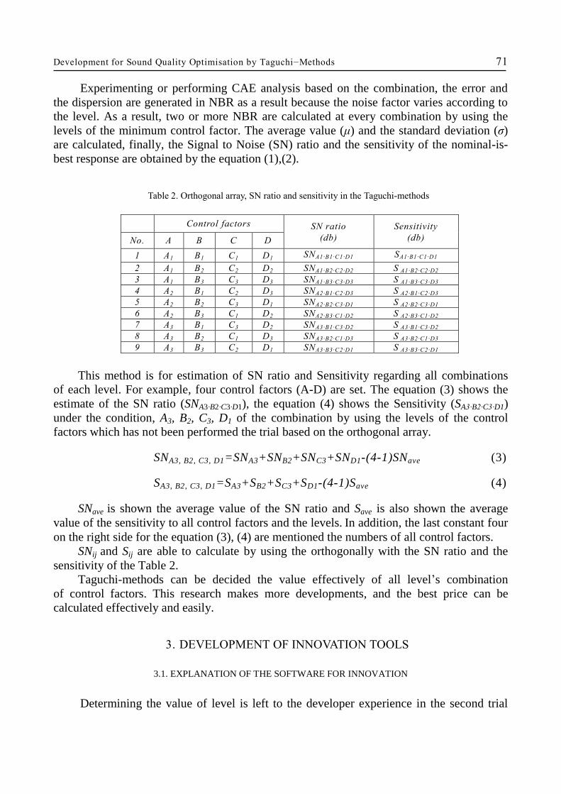
This method is for estimation of SN ratio and Sensitivity regarding all combinations
of each level. For example, four control factors (A-D) are set. The equation (3) shows the
estimate of the SN ratio (SNA3∙B2∙C3∙D1), the equation (4) shows the Sensitivity (SA3∙B2∙C3∙D1)
under the condition, A3, B2, C3, D1 of the combination by using the levels of the control
factors which has not been performed the trial based on the orthogonal array.
SNA3, B2, C3, D1=SNA3+SNB2+SNC3+SND1-(4-1)SNave (3)
SA3, B2, C3, D1=SA3+SB2+SC3+SD1-(4-1)Save (4)
SNave is shown the average value of the SN ratio and Save is also shown the average
value of the sensitivity to all control factors and the levels. In addition, the last constant four
on the right side for the equation (3), (4) are mentioned the numbers of all control factors.
SNij and Sij are able to calculate by using the orthogonally with the SN ratio and the
sensitivity of the Table 2.
Taguchi-methods can be decided the value effectively of all level’s combination
of control factors. This research makes more developments, and the best price can be
calculated effectively and easily.
3. DEVELOPMENT OF INNOVATION TOOLS
3.1. EXPLANATION OF THE SOFTWARE FOR INNOVATION
Determining the value of level is left to the developer experience in the second trial
Table 2. Orthogonal array, SN ratio and sensitivity in the Taguchi-methods
Control factors SN ratio
(db)
Sensitivity
(db) No. A B C D
1 A1 B1 C1 D1 SNA1∙B1∙C1∙D1 SA1∙B1∙C1∙D1
2 A1 B2 C2 D2 SNA1∙B2∙C2∙D2 S A1∙B2∙C2∙D2
3 A1 B3 C3 D3 SNA1∙B3∙C3∙D3 S A1∙B3∙C3∙D3
4 A2 B1 C2 D3 SNA2∙B1∙C2∙D3 S A2∙B1∙C2∙D3
5 A2 B2 C3 D1 SNA2∙B2∙C3∙D1 S A2∙B2∙C3∙D1
6 A2 B3 C1 D2 SNA2∙B3∙C1∙D2 S A2∙B3∙C1∙D2
7 A3 B1 C3 D2 SNA3∙B1∙C3∙D2 S A3∙B1∙C3∙D2
8 A3 B2 C1 D3 SNA3∙B2∙C1∙D3 S A3∙B2∙C1∙D3
9 A3 B3 C2 D1 SNA3∙B3∙C2∙D1 S A3∙B3∙C2∙D1

72 Hideki SAKAMOTO, Ikuo TANABE, Satoshi TAKAHASHI
that based on the first trial result as an issue even though Taguchi-method is known to be
that based on the first trial result as an issue even though Taguchi-method is known to be
able to use effectively in industries. Therefore, there is a case that the trial is repeated
several times if the selection of value is wrong. Thus the software which makes it possible
to develop industrial product rapidly and inexpensively according to search the optimal
combination of control factors for the best function in a short time by using Taguchi-
methods. Specifically, the software is calculated the factorial effect figures of the SN ratio
and the sensitivity by Taguchi-methods. Regarding the complete assumed events, it is
affected the function (intended characteristic value) as control factors in the first trial and
decides the optimal control factors and the level for the second trial. Then it is confirmed if
the combination is optimal in the second trial. The process which is decided the optimal
control factors and the level for the second trial is the original important part [3].
Table 3 Several examples for the control factors
Digital data Non-digital data
Item of the control factor Its properties Item of the control factor Its properties
Size, Weight,
Material and so on Design parameters
Product, Company,
Country, Individual data
Manufacturing condition,
Measuring condition,
Experimental condition
Action condition
National character, Worker,
Human nature, Animal,
Organic matter and so on
Personal data
Temperature, Humidity,
Air pressure, Weather,
Season and so on
Environment condition
Fig. 1. Effective figures of SN ratio and Sensitivity
(b) Sensitivity (=10 logμ2)
Digital data Non-digital data
123 123
Control factors
Levels
Sen
siti
vit
y
(db
)
●
● ●
●
●
●
(a) SN ratio ( =10log(μ2/σ
2) )
Digital data Non-digital data
123 123
Control factors
Levels
SN
ra
tio
(d
b)
●
●
●
●
●
●
Fig. 2. Types of curve in effective figures of SN ratio and Sensitivity
● ● ●
●
●
●
●
●
●
● ●
●
●
●
● ●
● ●
●
●
●
●
●
●
or etc
Flat Mountain Valley Combinations Picking up Picking down
Development for Sound Quality Optimisation by Taguchi−Methods 73
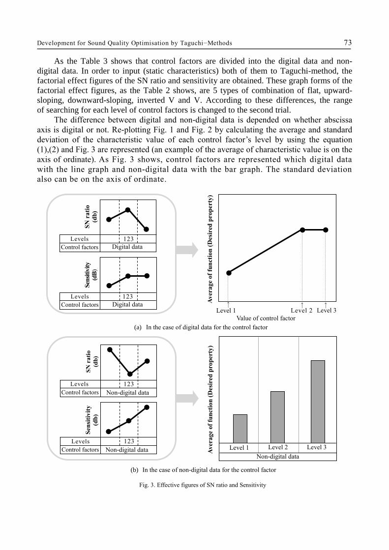
As the Table 3 shows that control factors are divided into the digital data and non-
digital data. In order to input (static characteristics) both of them to Taguchi-method, the
factorial effect figures of the SN ratio and sensitivity are obtained. These graph forms of the
factorial effect figures, as the Table 2 shows, are 5 types of combination of flat, upward-
sloping, downward-sloping, inverted V and V. According to these differences, the range
of searching for each level of control factors is changed to the second trial.
The difference between digital and non-digital data is depended on whether abscissa
axis is digital or not. Re-plotting Fig. 1 and Fig. 2 by calculating the average and standard
deviation of the characteristic value of each control factor’s level by using the equation
(1),(2) and Fig. 3 are represented (an example of the average of characteristic value is on the
axis of ordinate). As Fig. 3 shows, control factors are represented which digital data
with the line graph and non-digital data with the bar graph. The standard deviation
also can be on the axis of ordinate.
Fig. 3. Effective figures of SN ratio and Sensitivity
(b) In the case of non-digital data for the control factor
Level 1 Level 2 Level 3
Non-digital data
Av
era
ge
of
fun
ctio
n (
Des
ired
pro
per
ty)
Control factors
Levels
Sen
siti
vit
y
(db
)
Control factors
Levels
SN
ra
tio
(db
)
Non-digital data
123
●
●
●
Non-digital data
123
●
●
●
(a) In the case of digital data for the control factor
Value of control factor
● ●
Level 1 Level 2 Level 3 ↑ ↑ ↑
●
Av
era
ge
of
fun
ctio
n (
Des
ired
pro
per
ty)
Digital data
123
Control factors
Levels
Sen
siti
vit
y (d
B)
●
● ●
Digital data
123
Control factors
Levels
SN
ra
tio
(db
)
●
●
●

74 Hideki SAKAMOTO, Ikuo TANABE, Satoshi TAKAHASHI
As each level is not always distributed value when the inputted control factors are
digital data, it is common that the interval of each level is not distributed. According to
convert the factorial effect figures from the Fig. 1 into the Fig. 3, it is tended to image
physically the influence of each level for control factor. Moreover, the relation between the
magnitude relationship and the axis of ordinate value can be perceived a physical amount
correctly.
Table 4 Kinds of approximate curves regarding curve fit for first data in the software
Moreover, in case of the line graph of digital data as the Fig. 3, the relation between
each level of each control factor in the first trial can be smoothed by curve fit with five
types of approximating method as the Table 4.
The optimum levels of the control factors for the second trial are decided by applying
the results of the first trial. The method for selection of the optimum levels of the control
factors is shown in Fig. 4. In the explanation, it is supposed that the larger function is
desired for the designer. The curve of Fig. 4a has a mountain shape of graph, and there is
the optimum level of the control factor in the first trial. Therefore, new level 2’ is below in
the top of the mountain, new level 1’ is located in middle between the old level 1 and the
new level 2’, and new level 3’ is located in middle between the new level 2’and the old
level 2.
Fig. 4. Recommendation of the levels for 2nd trial using the results of the 1st trial
(1) Exponential approximation (4) Polynomial approximation
(2) Linear approximation (5) Radical approximation
(3) Logarithmic approximation (with degree)
Value of control factor
Level 1 Level 2 Level 3 ↑ ↑ ↑
Average
Level 1 Level 2 Level 3 ↑ ↑ ↑
Average
● ●
●
Level 1’ Level 3’
Level 2’
Result of 1sttrial
Recommended levels for 2nd
trial ●
Result of 1sttrial
Recommended levels for 2nd
trial ●
●
●
●
Level 1’
Level 3’
Level 2’
(a) Inside estimation (b) Outside estimation
Changeable and maximum value of the level in 2
nd trial
Av
era
ge
of
fun
ctio
n (
Des
ired
pro
per
ty)
Av
era
ge
of
fun
ctio
n (
Des
ired
pro
per
ty)
Value of control factor
●
●
● ●
●
●

Development for Sound Quality Optimisation by Taguchi−Methods 75
Level 1’, level 2’ and level 3’ are the optimum levels for the second trial. Moreover, the
curve of Fig. 4b has an ever-increased shape of graph, and there is the optimum level
of his control factor in the first trial correctly. Therefore, new level 3’ is decided as largest
value, new level 1’ and new level 2’ are located where divided three equal parts between the
new level 3’and the old level 3. The operator for the software can selected standard
deviation for vertical axis and estimate stability for the noise factors.
3.2. EXPLANATION OF THE EVALUATION METHOD OF SENSORY CHARACTERISTIC
Usually, the Sensory Characteristic Tuning Method is tuned with the alternative
characteristic. For example, in order to make a quality sound, the development which is
improved the characteristics such as a frequency response characteristic, S/N Ratio (Signal
Noise Ratio) and the THD+N characteristic as referred Fig. 5.
Fig. 5. Explanations of THD+D (Total Harmonic Distortion + Noi
However, these characteristic are static characteristic by the single signal at the specific
condition. Often there is a difference in the quality of the sound that their values and human
being feels in the actual sound source which is compounded continuous frequency. Also,
these characteristics would be changed due to fluctuations in the power supply.
The impedance, the level of a power supply and fluctuation of grand level are occurred
when circuit diagram is wired in advance. Since these are complicated composition, it is
also difficult for CAE to calculate.
Frequency
Amplitude
Harmonics
2nd 3rd
4th 5th
6th 7th
Signal
Noise
20kHz

76 Hideki SAKAMOTO, Ikuo TANABE, Satoshi TAKAHASHI
Therefore, it is tuned the constant of circuit by Sound Meister while listening to the
sound in advance. The way of tuning is depended on knowledge of each individual, but it is
difficult to manuals. In this research, it is an object to make tuning more efficient by
applying the innovation tool which cannot be manuals.
It has been found when human being listen to continuous sound, the difference
between listening sound and the true value of the sound are considered as the vector
difference of the m-dimensional [4]. Therefore, when listen in the columns is defined as Xd
and true value in the column is defined as Xs , the difference equation is following equation
(5).
Δ(R) = m-1/2
( Σ xdi2
+ Σ xsi2 ) (5)
By the above, human being can be captured RMS (Root Mean Square) as difference in
sound. As an indicator, when human being evaluates the sound, there is an indicator such as
senses of bass, treble and noise, etc. It is classified as a Table 5, and these values are
considered as RSM values. Thus, the comprehensive judgment shall be performed due to
calculate with the equation (6).
Table 5. Class zing and point of various indices
Excellent Good Fair Minimum Passing Failed
Score (xi) 5 4 3 2 1
Evaluation Score = Σ xi2 n = The number of indices (6)
Based on this theory, an actual product is evaluated which is based on eight indicators
on Fig. 6. The pass-fail judgment results of the product and this method results are matched.
Fig. 6. Result of the determination in the RMS value
m
i=1
n
i=1
m
i=1

Development for Sound Quality Optimisation by Taguchi−Methods 77
4. RESEARCH THROUGH THE OPTIMIZATION OF THE SOUND QUALITY
4.1. CONTROL FACTOR, NOISE FACTOR, AND MANUFACTURE CONDITIONS
In the end, the optimization of the Sound Quality of Optical Disc Drive is used for the
evaluation effectively with the innovation tool. It is aimed at improving the quality of the
Optical Disc Drive. Experimental system is shown in Fig. 7. Optical Disc Drive System
cannot be operated independently so that the system is necessary for the Sound Quality
evaluation to connect to standard Controller, Amplifier and Speaker exteriorly.
Fig. 7. Optical Disc Drive System Block Diagram
Motor
Pick-up
Zf
Zh
Ze
Zb
Za
Zc
μCOM &ServoDSP
Inte
rfac
eZd
Power Supply A
Power Supply B
Ground
Ground
LaserDiodeDriver
Zg
R2
R1
ServoDriver
ReferenceVoltage
LD Cont.
:Bleeder Resistor (R1 to R4)
:Characteristic ImpedanceZ
Ground
Reference Voltage
ActuatorDrive
LD Drive
MotorDrive
R3
R4
Fig. 8. Optical Disc Drive Control Panel Circuit
Servo DSP
Pick up
(Actuator / Laser Diode)
・Motor Drive
・Actuator Drive
・Signal
Optical Disc Drive Unit
Servo
ProcessorμCOM
Optical Disc Drive Control Panel
I/F
(to
Pro
du
ct)
・Mech. Control
・Audio outputDecorder
RF-AMP
・Laser Diode Drive
SERVO
DRIVER
Product
(Controller with AMP)
Motor
Optical Disc
PLAY 05:23
Speaker

78 Hideki SAKAMOTO, Ikuo TANABE, Satoshi TAKAHASHI
There are some factors which are determined the Sound Quality of Optical Disc Drive.
Therefore, design consideration in deliberation of factor is performed from early stages
of the design. In the optimization phase, it can be changed only small parts mainly Resistors
and Capacitors on the circuit board according to the design restriction.
As one of the factor to determine Sound Quality, it is generally known that affect to the
impedance characteristic by a circuit pattern and the current flowing along load. Usually, the
current impact cannot be detected by observation of the waveform. In the theory, dynamic
characteristic is normally identified to have an impact to Sound Quality so that it is possible
to improve Sound Quality in order to stabilize the current flowing same load.
Experimental circuit is shown in Fig. 8. Optical Disc Drive on Control Panel is used
for this experiment, and it is wired to be able to arrange Bleeder Resistor (R1, R2, R3, and
R4) in parallel with capacitor at power supply unit of four loads which has impact to Sound
Quality. Also, there is a possibility to vary the impedance of the circuit. Adjustment of the
Sound Quality is enabled by the constant of this Bleeder Resistor. In this experiment,
Evaluation Score of the Sound Quality is investigated for the combination which becomes
the largest. According to the innovation tool which is developed this time, the condition
search for improving the Sound Quality and the evaluation would be performed. The target
of evaluation score should be exceeded 8.49 as standard value which is referred to reference
products in the Sound Quality evaluation.
4.2. DETERMINATION OF THE LEVEL AND CONTROL FACTOR
Comprehensive evaluation of this software is performed to improve the Sound
Quality in the experiment of the condition search. The control factors for the first
trial are shown in Table 6. Four factors which is arranged Bleeder Resistor to
control impedance that have impact to Sound Quality by current flowing as the control
factors and three levels for each as Bleeder Resistor are set. Using L9 orthogonal array, it is
calculated with the static characteristic which is created the Evaluation Score to the
nominal-is-best response.
This experiment is conducted with nine experiments on the conditions which are
created to the control agent in L9 orthogonal array. It is calculated them like Section 2.1,
and the response graph for the SN ratio is shown in Fig. 9.
Table 6. Control factors for trial regarding the Optical Disc Drive for sound quality evaluation
Control factors
Name of factors Bleeder Resistor
R1 [ohm]
Bleeder Resistor
R2 [ohm]
Bleeder Resistor
R3 [ohm]
Bleeder Resistor
R4 [ohm]
Level 1 3.3k 3.3k 3.3k 3.3k
Level 2 10k 10k 10k 10k
Level 3 1M 1M 1M 1M
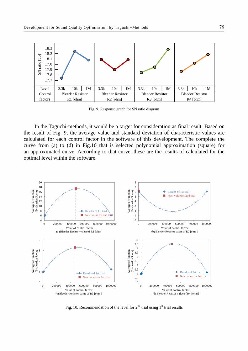
Development for Sound Quality Optimisation by Taguchi−Methods 79
Fig. 9. Response graph for SN ratio diagram
Fig. 9. Response graph for SN ratio diagram
In the Taguchi-methods, it would be a target for consideration as final result. Based on
the result of Fig. 9, the average value and standard deviation of characteristic values are
calculated for each control factor in the software of this development. The complete the
curve from (a) to (d) in Fig.10 that is selected polynomial approximation (square) for
an approximated curve. According to that curve, these are the results of calculated for the
optimal level within the software.
Fig. 10. Recommendation of the level for 2nd
trial using 1st trial results
Level 3.3k 10k 1M 3.3k 10k 1M 3.3k 10k 1M 3.3k 10k 1M
Control
factors
Bleeder Resistor
R1 [ohm]
Bleeder Resistor
R2 [ohm]
Bleeder Resistor
R3 [ohm]
Bleeder Resistor
R4 [ohm]
18.3
18.2
18.1
17.0
17.9
17.8
17.7
SN
rati
o[d
b]
4
6
8
10
12
14
16
18
20
0 200000 400000 600000 800000 1000000
Av
era
ge o
f fu
ncti
on
(Ev
alu
ati
on
Sco
re)
Value of control factor
(a) Bleeder Resistor value of R1 [ohm]
◆ Results of 1st trial
■ New value for 2nd trial
0
1
2
3
4
5
6
7
8
0 200000 400000 600000 800000 1000000
Av
era
ge o
f fu
ncti
on
(Ev
alu
ati
on
Sco
re)
Value of control factor
(b) Bleeder Resistor value of R2 [ohm]
◆ Results of 1st trial
■ New value for 2nd trial
5
5.5
6
6.5
7
7.5
8
8.5
9
9.5
10
0 200000 400000 600000 800000 1000000
Av
era
ge o
f fu
ncti
on
(Ev
alu
ati
on
Sco
re)
Value of control factor
(d) Bleeder Resistor value of R4 [ohm]
◆ Results of 1st trial
■ New value for 2nd trial
5
6
7
8
9
0 200000 400000 600000 800000 1000000
Av
era
ge o
f fu
ncti
on
(Ev
alu
ati
on
Sco
re)
Value of control factor
(c) Bleeder Resistor value of R3 [ohm]
◆ Results of 1st trial
■ New value for 2nd trial

80 Hideki SAKAMOTO, Ikuo TANABE, Satoshi TAKAHASHI
SN ratio of approximated curve has a combination of four resistance to be maximum
value that should be maximized Evaluation Score of Sound Quality in the second trial.
4.3. EVALUATION OF THIS SYSTEM
The combination for confirmatory experiment is showed that determined the
consideration of Section 4.2 in Table 7. The Evaluation Score of the Sound Quality for each
Tuning Method is shown in Fig. 11. Evaluation Score could be satisfied by applying both
the experiment of L9 along with Taguchi-method and the Software which is developed this
time. In addition, the result is equivalent to determine the level with Try & Error method
which is performed by the Sound Meister.
By the conventional method, total 150 examinations are required in order to reach the
target. On the other hand, this method is ended by 10 times to be able to optimize for
equivalent values. Thus, it is performed efficiently to achieve to the target, and the number
of time is gone up to 15 times.
According to this examination, the second trial is required only to check the status.
The reasons are that; (1) Based on the first trial result, the control factors and the level for
the second trial could be promised a certain level of effect (2) Narrowing down of a constant
would be difficult because the sensitivity of factor is become high.
Table 7. Results of the resistance value calculated
Resistor R1 [ohm] Resistor R2 [ohm] Resistor R3 [ohm] Resistor R4 [ohm]
470k 3.3k 470k 470k
Fig. 11. Comparison of the results
7.36
8.53 8.52
6.8
7.0
7.2
7.4
7.6
7.8
8.0
8.2
8.4
8.6
Before Tuning Using Taguchi Method Try & Error method
Ev
alu
ati
on
Sco
re
Target Score

Development for Sound Quality Optimisation by Taguchi−Methods 81
5. CONCLUSION
From this research, it could be concluded that; (1) Sensory characteristic tuning method
by using Taguchi-methods is calculated the values to be optimized in a few studies, and the
result is equal to or greater than the result of Sound Meister is implemented. (2)
Commonly, the sensory characteristic of optimization is conducted with Try & Error
method; however, it is confirmed that leading the improvement of productivity by using this
method.
REFERENCES
[1] TATEBAYASHI K., 2005, Computer Aided Engineering Combined with Taguchi-methods, Proceeding of the 2005
Annual Meeting of the Japan Society of Mechanical Engineering, 8/05−1, 224−225.
[2] SUGAI H., TANABE I., et al, 2006, Prediction of Optimum Machining Condition in Press Forming Using
Taguchi-methods and FEM Simulation, Transactions of the JSME, 72/721, 3044−3050, (in Japanese). [3] TANABE I., IYAMA T., HOANG VU L., 2011, Evaluation of influence regarding control factors using inverse
analysis of Taguchi-methods (Influence regarding organic matter in control factors), Transactions of Japan Society
of Mechanical Engineers, 77/780, 3117−3126.
[4] NEMOTO I., 2011, Discussion on Methods of RMS Comparison of Evoked MEGs, The 49rd Annual Conference
of Japanese Society for Medical and Biological Engineering, 3, 516−521.
Recommended
![DEVELOPMENT OF PERFECTLY DESIGN SYSTEM USING TAGUCHI METHODS · 70 Hideki SAKAMOTO, Ikuo TANABE, Satoshi TAKAHASHI estimate the optimum combination of design parameters [4] as the](https://img.dokumen.tips/doc/110x75/5b47bc3e7f8b9af54b8c61ab/development-of-perfectly-design-system-using-taguchi-70-hideki-sakamoto-ikuo.jpg)