RD-RI54 752 ONR ANNUAL REPORTMU YALE UNI NEW HAEN CONN KLINE
1/1GEOLOGY LAB 29 OCT 84 NOee4-82-K-037i
UNCLASSIFIED F/0 8/10 NL
I hhhhhhh
%
12.2
11111 1.1&0___-
S1.25 111~ ll
MICROCOPY RESOLUTION TEST CHARTNATIONAL BUREAU OF STANDARDS- 1963-A
Diepartm of Cetiloy @"d Grophysm~ Compu., addresY l U nv riyKline Geolog) LaI'oratery Kline Geology LaboratoryYale University "0 ;~hlYAeu
P.O. box 6666 soo Rime,,y AvueuNew, Have", Conrair, .S11t Telephone
aej 46.aD8 . ,
InDr. Tom SpenceONR DET Code 422P0Office of Naval Research
L Arlington, VIRGINIA 22217October 29, 1984 .
Ref No: N00014-82-K-0371Dear Ton:
I am sending you an annual report mostly in pictures. I chose the topicswhich could be more easely explained by the figures and that summarize the .approach we are taking. George is in Australia and the secretaries are onstrike. I had to cut and paste because I cannot find the originals. I hope itwill serve the purpose.
There are many subtle points that I could elaborate on, but it seemed tome that you would prefer more pictures than text. I kept the text to a Snecessary minimum to make the figures understandable. The published papersgive all the details, so it would be unnecessary duplication. I hope themessage is understandable.
Thank a lot for your help
Manuel Fiadeiro.
Research Scientist, -Yale University.
L)TICC.2 ELECTEUJSJUN 10 85
LLIa
This document has bee aoedt 85" 5 13 094jot public telease and sale; its
distiibution is unlimited.
ONR ANNUAL REPORT - OCTOBER 1984
Ref .no.N00014-82-K-0371 "
A) THE SEARCH FOR THE LEVEL OF NO NOTION
The inverse method applied to the mass conservation equations is a
powerful method to obtain, from a set of oceanographic stations, a velocity
field in geostrophic equilibrium obeying the conservation constraints imposed.
The solution is a barotropic field that represents the absolute velocity at a
given reference level. If there are less constraints than station-pairs, the
problem is underdetermined and there are an infinite number of solutions. In
these circunstances one has to choose which solution to adopt.
It has been the practise, for the purpose of calculating the absolute
velocity field, to assume a level of no motion within the water column. This
heuristic assumption has been implemented in many ways. The inverse method
provides a mathematical formulation and a quantative way to assess this
assumption.
If a level of no motion exists and the mass constraints are obeyed it is
reasonable to assume that the transport imbalance relative to that level
should vanish. Due to errors in the data we can expect instead a small
variance from zero. We proposed a procedure in which the reference level is
changed from the surface to the bottom, to search for the minimum magnitude of
the transport imbalance vector. This procedure gives a good estimate of the
mean level of no motion and in most cases, acceptable residues for the
imbalances.
We can also use the projection matrix of the parameter space (the
resolution" matrix) to look for the level that gives the smallest of the
minimum norm solutions. These two procedures give a "best" reference level no
more than 100m apart. In most cases the residual error and the variance of the
solution are within acceptable limits and no correction is necessary. Examples
are shown for the Coral Sea (Gascoyne 2/60, 1962) and Bermuda triangle
(Atlantis 215, 1955)datasets.
The Bermuda triangle needs special mention. Here we divided the water
mass in five layers. The upper two layers contained shallow stations at which
1i11
we assumed zero velocity at the bottom (OV stations). Some of these stations 0
are across the Gulf Stream were this assumption is most likely to be false.
Thus, we could expect large imbalances for those two layers. We then calcu-
lated the residual transport for the bottom three layers including only those
stations with a maximum depth near or below the reference level. The search
procedure gave us a best reference level at 3500m. The imbalance of the upper
two layers was then attributed to the OV stations and an inverse solution was
found for them. The resulting Gulf Stream transport across the Ft. Pierce
section became comparable with the measured flow. P.
As a final note we restate that these results are not a proof that a
level of no motion exists. They only show that there are solutions compatible
with a level of no motion. While the problem is underdetermined there will be
an infinite number of solutions. The inverse solutions are projections of the
true solution into a subspace of the parameter space. We have access only to a
limited representation of the solution, but at least, this representation
should vanish if the assumption is true. So far, we have always found a
solution compatible with a level of no motion and have presented the
baroclinic field relative to that level as the most probable absolute velocity
field.
Publications:
On the determination of absolute velocities in the ocean by Manuel E.
Fiadeiro and George Veronis. J. Mar.,Res. 40(sup.),159-182,1982.
see also: Conmients on "On the determination of absolute velocities in the Iocean" by L.L. Fu and Reply to L.L.Fu J. Mar. Res.,42,259-262,1984.
Circulation and heat flux in the Bermuda Triangle by M.E. Fiadeiro and
George Veronis. J. Phys. Ocean.,13,1158-1169,1983.
2
.. .. . . .. . . . . . . . .
CORAL SEA
50 10 50 M0 IM 5050..
-.-
.--
Zr 300 - oIGFA. Nj.t' ~----ml-"--
5000
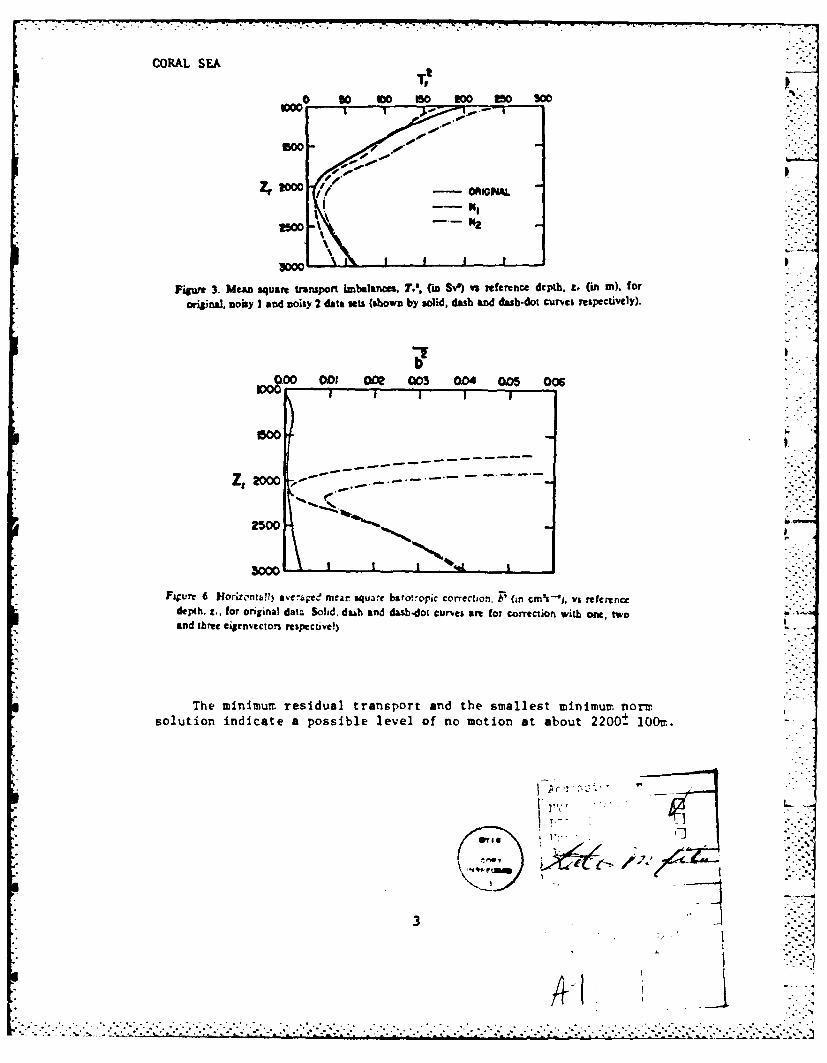
Figure 3. Mean square transport imbalance, T'. (in Sv") vs reference depth, 1. (in m). fororiginal, noisy I and noisy 2 data sets (shown by solid, dash and dash-dot curves respectively).
~ 0 001 we~ a03 04 005 0
MOW
25D0
FaIurr 6 Morizontall s aee mear aqua% barotropic correction. G'(n cM%'). vs referencedepth, z,, for original data Solid. dash and dub-dot curves wre for correction with onse. twoand threc eigenvtoors respec~ivel)
The minimumt residual transport and the smallest minimum~ norm'.solution indicate a possible level of no motion at about 2200t loome.
rL
4LL
......-T.
. . .. . . .. •
- --. ~ .- .- -.-..-:-_-. -.................. .
K . CORAL SE.A
W~~M S W MS 8
20.o*1 g.3
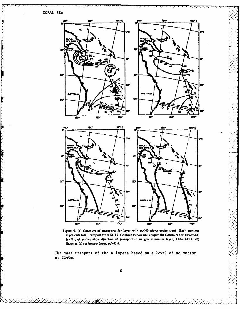
Fiur 9 () onous f rasprt fr ayr it @< 4 aon cuie rak ac cntu
ftreft ttl rnsot rm t 3.Coturcrvsso niu; b Cnousfo OM<I
(C)Bradarrwsshw iretin f ranpot n oygn inmumlaer 4Cem414;(d
Sameas () fo botom lyerea)41.4
The asstrapor ofthe laersbasd o a lvelof o mtioat rR 2140m.U
541
BERMDA TRIANGLE r2 4 68 9 o
20am22I.
so3 - -
34- 36
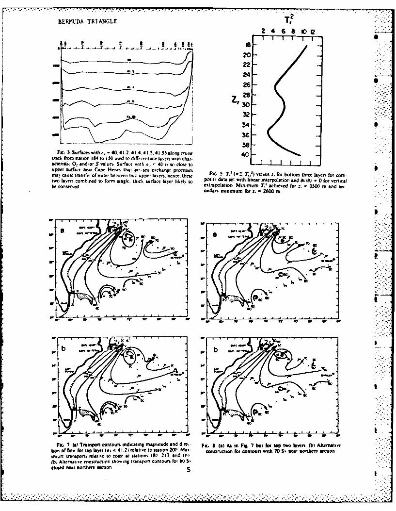
38Fic, 3.Surfaceswth,)-40,41.2.41.4.4.S,.4l mlon cruise 40r
track from station 15410o 130 used to~ differentiate IaWrr %%itti char-Saltnstit 0. arad'or S values. Surface with ve. 40 is so close to I I Iupper surface near Cape Her that air-sea exchanilr processes . ,ST 2
( ,' v~u: o otmthe aesfrcmma' cause transfer of water between two upper lav~ers, hence. thew I.572 T,)viefrbto heelyr.frcmtwo layers combined to form singic, thick surface laver liaelh to poste data sot with linear interplation and a./O: - 0 for vertical
be onervdxtraPolation Minimum V, achieved for,- 3W0 m and sec.ondaxn minimumn for x. *2600 in.
4pew W
Bar or
W 1DK9U,6
Vo br
a..P
3C 41C
or s
a.PC
W r 1
clse nerortenstto
IT......................................... . . . . .
B) THE INVERSE PROBLEM WITH TRACER MIXING
Figure 1 shows theqj and PV (fJ) vertical sections along the meridian
50W, Atlantis cruise ATL 229. To the left, St.5416 Is off the Grand Banks and
to the right, St.5471 is off the French Guiana. The section closes a large
section of the Atlantic Ocean, the Caribbean and the Gulf of Mexico.
The assumption that properties are conserved by layers cannot hold for
such large bodies of water. To the south (right), the water masses present a
characteristic combination of 03 and PV found nowhere else. To the north, the
deep water between 1000 and 3000m has an homogeneous PV-O 8 . Between Sts.
5436 and 5449 a minimum PV at C304.7 marks the body of 180 water that has
annual contact with the surface further east and to the north. In such
circunstances one would be hard pressed to choose conservative layers. It is
obvious the different water masses are being mixed inside the region closed by
the section.
This example points out the need to include mixing effects in the formu-
lation of the inverse problem if we hope to obtain any meaningful results. To
that purpose we undertook a theoretical study of the mixing effects on the
inverse procedures.
We started our study with two-dimensional tracer distributions generated
by a model. We used an extremely simple flow field (a constant flow from left
to right) and a constant eddy diffusion coefficient. The direct problem was
solved in a grid of 16x64 points. For the inverse problem a small region of
6x6 points is sampled and treated as observed data.
In figures 2 to 7 the original flow field would be represented by
equidistant streamlines with a value of 0 at the bottom and 4 at the top. We
show the result of different procedures.
Flg.2 shows solutions of underdetermined systems, using the equations foronly one tracer; c1 and c2 are different tracers and (5,7) and (23,6) refer to
the sampling region of the direct solution. The solutions are entirely
different from the input flow field. The patterns change with the tracer used
and region sampled. These are minimum norm solutions; we can retrieve the
original flow field by using two tracers or one tracer and additional correct
constraints to make the problem well or overdetermined.
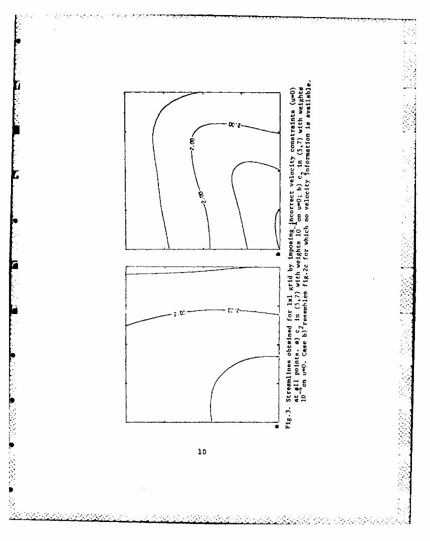
Fig.3 represents an interesting case. We added incorrect information
(u-) to the system; a) with a weight of 10"1, b) with a weight of 10-4. The
6
.... . * .- .. ..., ... . . . . . .* .. * .. . - '

streamlines change with the weight of the velocity constraints. As the weight
decreases the pattern tends to the minimum norm solution shown in fig.2c. This
is in contrast with the cases where we added correct information; the correct
streamfunction was retrieved independently of the weight of the velocity
constraints. This can prove to be a very useful technique In practise:
orthogonal" information compatible with the tracer is accepted by the system
but incorrect information that conflicts with the tracer is rejected by the
system.
In practise, data have errors and the parameters are mean properties of
the field for the scale of the observations. We added random noise and sampledthe model data at every other grid point. In these circunstances the model
parameters give residuals to the equations and the inverse procedure finds a
solution with even smaller residues. The question is to determine how far is
the solution from the expected parameters of the model. The underdetermined
cases were hopeless, the residues can be made to vanish but the solution has
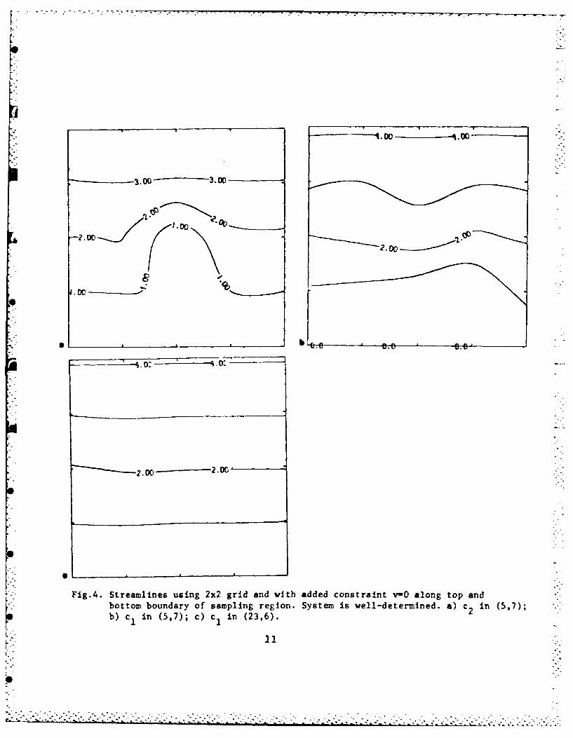
no physical significance. Fig.4 shows solutions of strict well-determined
systems. We added to the tracer equations the condition v-0 at the bottom and
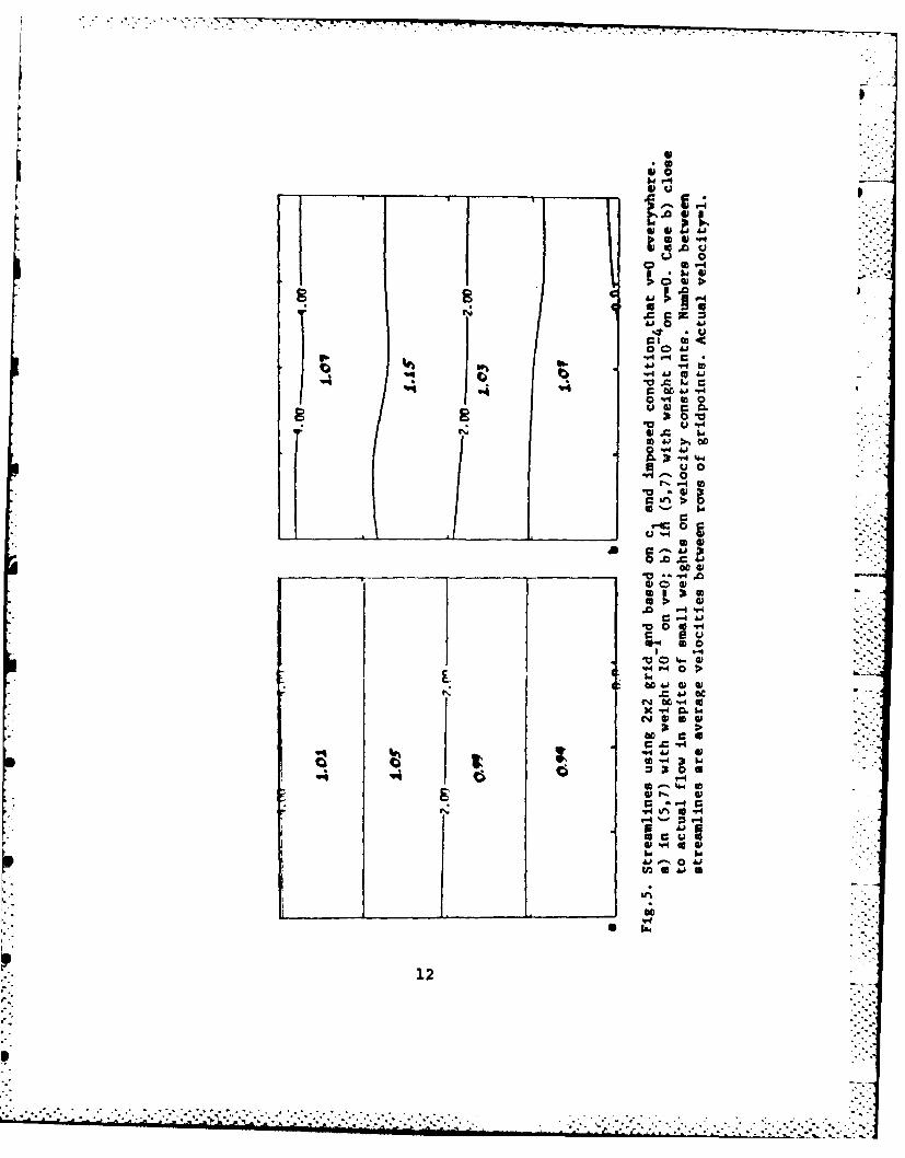
top of the sampling region. Fig.5 shows solutions when we impose vO all over
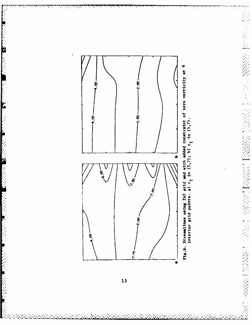
the sampling region (the system is overdetermined). In fig.6 we show solutions
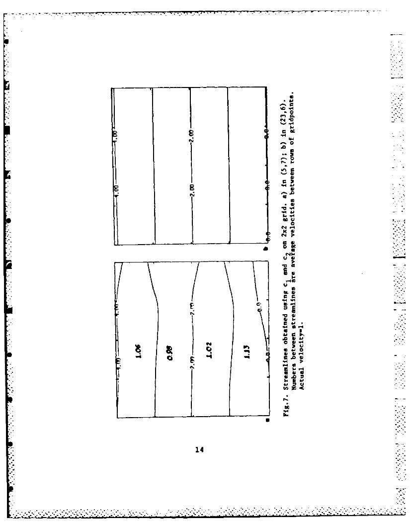
with a no vorticitty condition for the 9 interior points ( --=O -%=O) and infig.7 solutions with two tracers. As can be seen, under certain conditions,
overdetermined system (least-squares solutions) can give reasonable
approximations of the expected flow field. As a rule of thumb, we found out
that if the inverse of the condition number of the coefficient matrix is
smaller than the mean residue square of the equations, the solutions are very
good approximations of the expected velocity field; otherwise, one should be
extremely careful to interpret to results.
Regarding the application to oceanographic data, we can know very
precisely the condition number of the inversion matrix, once the problem is
set up; but we lack a good estimation of the errors in the data. We are
presently working on this problem.
7. . .. . .. . . . . . .-.

49 .... ...
IY
Fig.1. 47(above) and PV (below) for the 50*W section of ATL229.
3
4M
Unique combinations of rand PV Indicate mixing effects in theportion of the ocean closed by the section.

.00
3.0000K
* Fig.2. Stream~lines obtained from inverse calculation for underdetermiined system withsingle tracer in indicated sampling regions. a) c1 in (5,7); b) cin (23,6);c) c 2 in (5,7); d) c 2 in (23,6).
W.4
UC>
0 r
C• .' 0
.4.4 .4.44.
I U
o u
W .
0 10
C
0
4-4gu
10.'.,
.. 0
i:"- -:.: -: .-,. -:.. .:. :--,-'.: -,, -.:-.. - .- .,. , ..--.-. .- .. .. . , . .~ -. .. . . ... .. . - .... . .... .. ,o _ . . ... . . . _ , _. . . . .. :j . -." .. .._ ._. .; .. .;. ; .. . -. . -; .;. -_ .-. ..- .-. ... -.. ;
3.0 3.00
1.0 Ci2
2.00 D
Fig.4. Streamlines using 2x grid and with added constraint v-0 along top andbottom boundary of sampling region. System is well-determined, a) c2in (5,7);b) c1 in (5,7); c) c1 in (23.6).
10
S 0 0
u* 0
C
40 0I
CO 48
W~h -44
v0
0 oo
C 1-4'* >
Aj 4
-4
N -4 k k b -A
W aW
V4
'4 ' "44120
0%
-r
AI
13.
tq44*0
C4
4.6
10
SC4".
c.0 4
ol 1-4
_ _ _ _ _ )
14a
Publications.
Obtaining velocities from tracer distributions by M.E. Fladeiro and
George Veronis. submitted to J. Phys. Ocean.
Inverse methods for ocean circulation by George Veronis. Advanced Study
Institute Lectures, Scripps Institution of Oceanography. In press
An overview of the inverse method in oceanography by M. Fiadeiro (for
publication).
Principal Investigators.
George Veronis and Manuel E. Fiadeiro
Department of Geology and Geophysiscs. Yale University.
P.O. Box 6666. New Haven, Connecticut 06511
Phone: (203) 436-1078 / 436-8015
Contract no.: N00014-82-K-0371
Title: Expanded study of the inverse problem for ocean circulation.
.e -'-
151
.. . . . . . . . .... . . . . . . . . . . . . . . . . ... 4 ( *.~s ~. ~ . * * ~ .- ,*.* - .. - - - -
i,..K:
AI
S.
FFILMED.V.,
4.
7-85
DTIC. . . . .
.................................................. .. ..
.....................................
Recommended

![Chris J. Myers - University of Utah J. Myers (Lecture 5: ... uu dd r HH$$ HHH HHH H PRO r r3OO p ... VVVVVVV VVVVVV CIII r m hhhhhhh hhhhhhh hhhhhh k10·P1tot ·k8/k9 [CII]](https://img.dokumen.tips/doc/110x75/5aedfa177f8b9aa17b8bae48/chris-j-myers-university-of-j-myers-lecture-5-uu-dd-r-hh-hhh-hhh-h-pro.jpg)