HF WIRE ANTENNA ARRAYS
NUMERICAL SIMULATIONS
&
DESIGN GUIDELINESS
Dr. Levent Sevgi
March 1999
i
SUMMARY
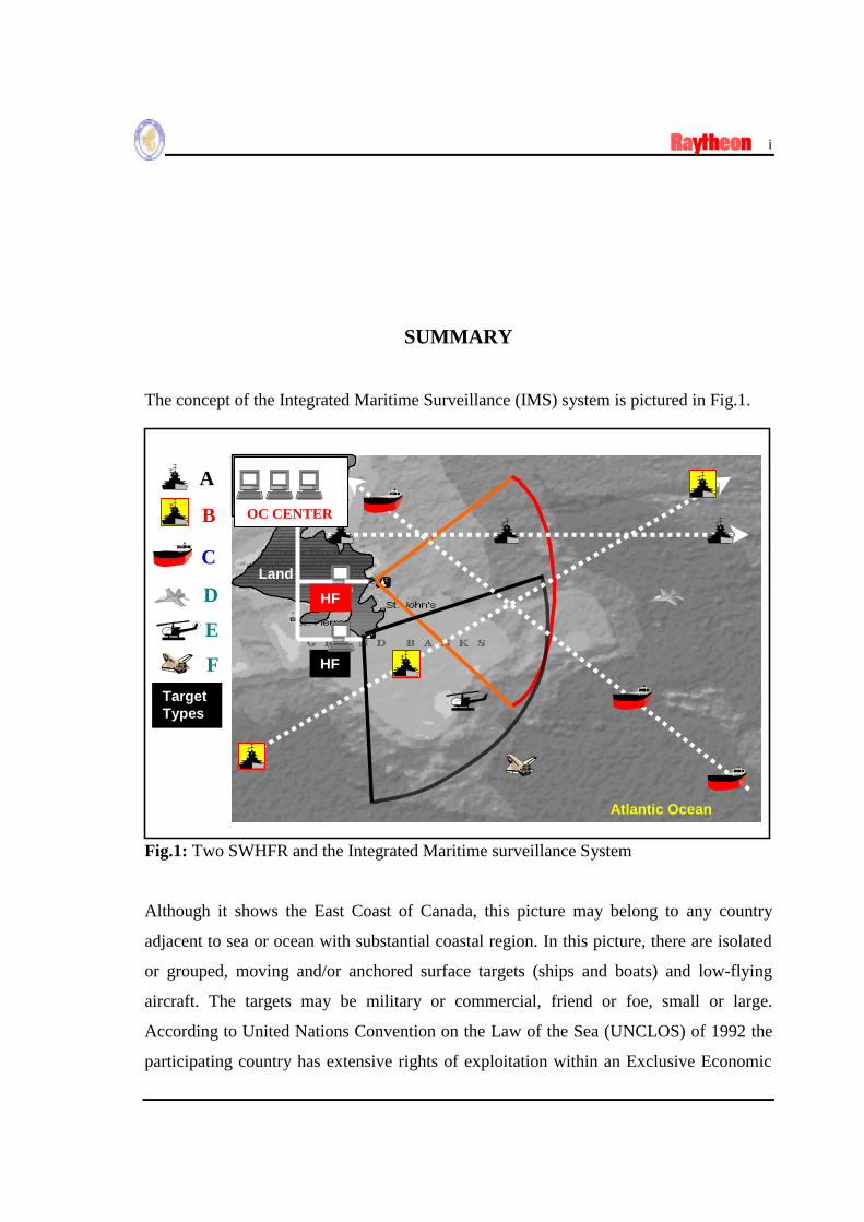
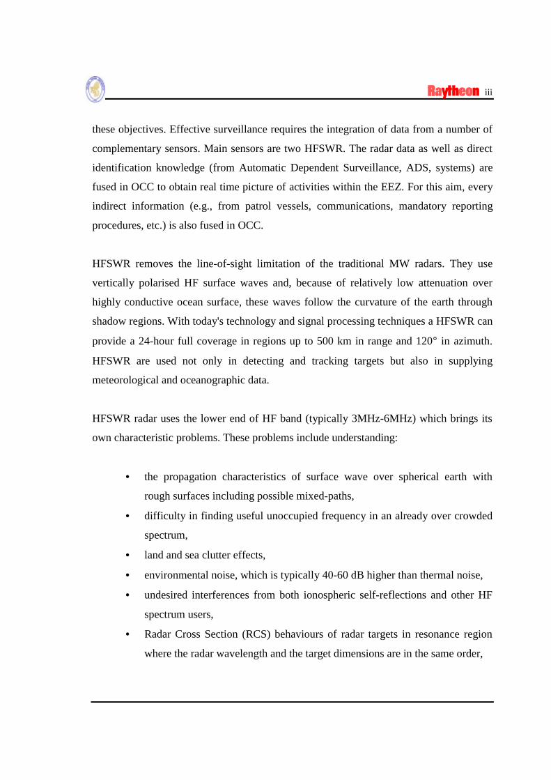
The concept of the Integrated Maritime Surveillance (IMS) system is pictured in Fig.1.
Fig.1: Two SWHFR and the Integrated Maritime surveillance System
Although it shows the East Coast of Canada, this picture may belong to any country
adjacent to sea or ocean with substantial coastal region. In this picture, there are isolated
or grouped, moving and/or anchored surface targets (ships and boats) and low-flying
aircraft. The targets may be military or commercial, friend or foe, small or large.
According to United Nations Convention on the Law of the Sea (UNCLOS) of 1992 the
participating country has extensive rights of exploitation within an Exclusive Economic
Atlantic Ocean
HF
A
B
C
D
E
F
OC CENTER
HF
Land
TargetTypes
ii
Zone (EEZ) which extends up to 200 nautical miles (nm) from shore. Beside the
economic benefits, a participating country carries responsibilities such as prevention of
smuggling, terrorism and piracy, the effective management and protection off-shore
fisheries, search and rescue, vessel traffic services, pollutant control and meteorological
and oceanographic data collection.
The questions behind the IMS idea are simple. How could this picture be reflected on a
computer monitor in an Operation Control Centre (OCC)? What would the reliability of
the picture be and how close would the OCC picture be to the real one? Do all the targets
in EEZ appear in this picture? Are there any virtual targets? Are all the targets classified
and identified? Although answers for all these questions are extremely complex, the key
issue in developing the IMS system is simple; a better understanding of the physics
behind this concept. In order to bring the IMS system to reality, electromagnetic wave -
ocean wave interaction, surface and sky wave propagation characteristics, target
reflectivity, undesired interference sources must all be very well understood.
What are the alternatives to monitor EEZ? Traditional land-based microwave (MW)
radars are limited with the line-of-sight, which means a maximum range of 50-60km even
with the elevated radar platforms. The EEZ can be covered by a MW radar in a patrol
aircraft, but requires three to five aircraft (well above 20,000ft) with many hours on
station. Satellites have neither the spatial nor the temporal resolution to provide this
surveillance in real-time. Sky wave high frequency (HF) radars can be used for this
purpose, but they need huge installations, are extremely expensive and detection of
surface targets is still limited.
The optimal solution is IMS. IMS uses HFSWR as the primary sensors. The requirements
of the IMS system based on HFSWR radars are two-fold. First; to detect, track, classify
and identify targets on and above the ocean surface out to 500km. Second; to remotely
sense and map surface currents, winds, sea state and ice. No single sensor can achieve all
iii
these objectives. Effective surveillance requires the integration of data from a number of
complementary sensors. Main sensors are two HFSWR. The radar data as well as direct
identification knowledge (from Automatic Dependent Surveillance, ADS, systems) are
fused in OCC to obtain real time picture of activities within the EEZ. For this aim, every
indirect information (e.g., from patrol vessels, communications, mandatory reporting
procedures, etc.) is also fused in OCC.
HFSWR removes the line-of-sight limitation of the traditional MW radars. They use
vertically polarised HF surface waves and, because of relatively low attenuation over
highly conductive ocean surface, these waves follow the curvature of the earth through
shadow regions. With today's technology and signal processing techniques a HFSWR can
provide a 24-hour full coverage in regions up to 500 km in range and 120° in azimuth.
HFSWR are used not only in detecting and tracking targets but also in supplying
meteorological and oceanographic data.
HFSWR radar uses the lower end of HF band (typically 3MHz-6MHz) which brings its
own characteristic problems. These problems include understanding:
• the propagation characteristics of surface wave over spherical earth with
rough surfaces including possible mixed-paths,
• difficulty in finding useful unoccupied frequency in an already over crowded
spectrum,
• land and sea clutter effects,
• environmental noise, which is typically 40-60 dB higher than thermal noise,
• undesired interferences from both ionospheric self-reflections and other HF
spectrum users,
• Radar Cross Section (RCS) behaviours of radar targets in resonance region
where the radar wavelength and the target dimensions are in the same order,
iv
• the problems of large transmit and receive antenna arrays located over lossy
ground.
The first step in finding solutions to almost all of these problems is designing suitable
antenna systems. Good antenna system design will
• improve directivity, gain and surface wave coupling to reach longer ranges,
• enlarge azimuth coverage,
• increase front-to-back ratio to minimise interference originates sources behind
the array and back-located site interferences,
• provide deeper over-head null to reduce self-generated ionospheric interferences,
etc.
The design parameters of a HFSWR antenna system are
• Operating frequency bandwidth
• Maximum Directivity and Gain
• Maximum Front-to-back ratio
• Maximising over-head null
• Vertical and horizontal radiation patterns.
HFSWR antenna systems are located on earth’s lossy ground, where the bore-sight points
the centre of azimuth coverage. The electrical parameters of the ground play a critical
role in antenna performance. Typical parameters for Good Land and Poor land are
εrg=15.0, σg=0.01 S/m and εrg=4.0, σg=0.003 S/m, respectively. On the other hand, ocean
parameters are εrg=80.0, σg=5.0 S/m. At HF frequencies the smooth ocean surface acts
almost as a perfectly electrical conductor (PEC). A vertical monopole with length l over a
PEC surface acts as a dipole with an equivalent length of 2l in free-space. Therefore, a
quarter-wavelength monopole over PEC acts as a half-wavelength dipole in free-space.
v
The angle between the horizontal plane and the vertical radiation maximum is called the
take-of-angle (TOA). Vertical monopoles over PEC surface have a 0° TOA. As the
surface loss increases TOA also increases.
A vertical monopole element has a donut radiation characteristic. That is, isotropic in
azimuth plane with horizontal maximum and vertical minimum radiation. However, when
placed over lossy ground the horizontal maximum tilts up to between 25° to 40° and the
antenna gain reduces by 10dB to 15dB, depending on the ground parameters.
To compensate ground losses and to lower TOA (so, more EM energy may couple over
ocean surface) ground screens under the antennas are used. The aim of ground screen is
two-fold. First, it stabilises the input impedance of each monopole over the entire
frequency band, which results compensation in antenna gain. Second, it increases the
surface impedance, so that vertical element has a better image and lower TOA to allow
more surface wave coupling. Depending on the crucial needs a variety of ground screens
may be designed. Some general rules may be listed regarding to ground screen design:
• If the gain is crucial, then stabilising the elements’ input impedances is
essential. It may be done either by locating circular or rectangular PEC
patches under each vertical monopole element or using by radial wires.
• If lowering the TOA is crucial, then using horizontal wires that are
perpendicular to antenna bore-sight seems to be the most proper solution. In
this case, horizontal wires should extend at least quarter-wavelength at each
side, half-wavelength at the back and a wavelength in the front.
• If the over-head nulling is the most important requirement, keeping the
antenna array and ground screen depth (i.e., the size of the array along bore-
sight) and avoiding complex wiring in the ground screen layout are necessary.
The more complex the wire connections the higher the diffractions and the
lesser over-head nulling property.
vi
The general design guidelines for HFSWR antenna systems may be outlined as:
• Use structures as simple as possible (to avoid electromagnetic complexity)
• Use vertical monopoles (for better over-head nulling)
• Locate the array as close to shore as possible (to reduce mixed-path loss anddiffraction)
• Level the ground as much as possible (to reduce diffraction effects)
• Keep channel depth as short as possible (to reduce ionospheric clutter)
• Use simple ground screen layouts (to reduce ionospheric clutter)

vii
SUMMARY i
CONTENTS vii
I Introduction 1
II Time and Frequency Domain Numerical Techniques 3
2.1 Finite-difference Time-Domain method 32.2 Method of Moments 6
III Receive Array Channel Elements 12
3.1 Quadlet, Triplet and Doublet with monopoles 123.2 Quadlet, Triplet and Doublet with fat monopoles 243.3 Crossed Monopoles 34
IV Receive Arrays 38
4.1 Seven-element array 384.2 Sixteen-element array 424.3 Twenty four-element array 44
V Ground Screen Design 47
VI Design Guidelines and Conclusions 55
1
I Introduction
The Integrated Maritime Surveillance (IMS) system basically relies on the information
obtained from two HF surface wave radars (HFSWR) to 24-hour continuously monitor
large ocean areas. Therefore, the information supplied from HFSWR to IMS is the key
issue for system reliability and performance. The main sub-systems in the HFSWR are
• The transmitter and receiver sub-systems
• The signal processing unit
• The HF spectrum monitoring unit
• The operation control centre (OCC).
Since the HFSWR operation is based on electromagnetic (EM) reflectivity of surface and
air targets in the coverage area, EM surface wave producing by the transmit antenna
system and target-reflected EM wave capturing by the receiver antenna system are very
important. The transmit and receiver antennas are systems, which satisfy the physical
requirement essential for the reliability in SHFSWR.
Both transmit and receive antennas of HFSWR are compound of vertical monopoles
located over earth’s lossy ground under which certain ground screen layouts are used.
The mission of the transmit antenna system are
• to couple as much EM energy as possible over the sea surface,
• to give as much gain as possible over the desired frequency band,
• to give as much front-to-back ratio as possible over the desired frequency
band,
• to cover azimuth range up to 120°,
• to have as deep over-head null as possible, in order to get rid of ionospheric
self-interference effects.
2
Similarly, the receive antenna system missions are
• to cover azimuth range up to 120°,
• to give as much front-to-back ratio as possible over the desired frequency
band,
• to have as deep over-head null as possible, in order to get rid of ionospheric
self-interference effects,
• to allow electronic beam steering abilities as close to theoretical behaviours as
possible.
In this report, HFSWR antenna systems are overviewed. First, Cape Bonavista and Cape
Race transmit and receive arrays are investigated. The channel elements of both sites are
analysed over lossy ground without and with ground screens. A doublet, a triplet and a
quadlet are used as channel elements for both Cape Bonavista and Cape Race receive
arrays and their performances are numerically simulated. Different radiators are used as
channel elements, such as monopoles, fat monopoles and inverted cones. Then, a seven, a
sixteen and a twenty-four channel arrays are analysed and electronic beam forming
capabilities are investigated. Finally, the conclusions are outlined together with major
design guidelines.
Two well-known numerical techniques are used for these simulations. They are the
Finite-Difference Time-Domain (FDTD) and Method of Moments (MoM) techniques.
FDTD is a time domain technique where broad band frequency behaviours can be
obtained via a single simulation. MoM is a frequency domain technique where complex
structures over lossy ground with different ground screen layouts can easily be
investigated. While in-house written FDTD code is used for FDTD simulations,
commercially available NEC2 package is used for MoM simulations.

3
II Time and Frequency Domain Numerical Techniques
Broad class of complex EM problems can be handled via a few time and/or frequency
domain techniques. In this section, FDTD and MoM techniques will be outlined.
2.1 Finite-Difference Time-Domain Method
This method is based on the
discretization of Maxwell’ s two curl
equations directly in time and spatial
domains and divide the volume of
interest into unit cells as shown in
Fig.2.1. This unit cell is called Yee cell
[1] where electric and magnetic field
components are located at different
places. For the numerical implementation
of FDTD method, the observations listed
below are made:
• There are three electric and three magnetic field components in each Yee cell
which is distinguished by (i, j, k) label. The discretization steps are ∆t and ∆x,
∆y, ∆z for time and position, respectively which gives the co-ordinate (i, j, k)
and the time n as
(i, j, k) = (i×∆x, j×∆y, k×∆z), t = n×∆t (2.1)
(for clarity, the time index n is suppressed and unless otherwise is stated the
field components are given for time n, i.e., Ex=Exn).
• Although field components in each cell are labelled with the same (i, j, k)
numbers (such as Ex (i, j, k) or Hz (i, j, k)), their locations are different.
F ig.2 .1 : Y ee ce ll fo r th e F D TD m e th od

4
• Besides the location difference between field components in a cell, there is
also a time difference between electric and magnetic field components. That
is, the electric field components are calculated at time steps t=∆t/2, 3∆t/2,
5∆t/2, …..
• Both magnetic and electric field components in any cell may be moved to
origin by just cell averaging. This is accomplished by using two magnetic
field components as;
[ ])k,j,1i(H)k,j,i(H2
1)k,j,i(H xxx ++×= (2.2)
but four electric field components as;
[ ])k,1j,1i(E)k,1j,i(E)k,j,1i(E)k,j,i(E4
1)k,j,i(E zzzzz +++++++×= . (2.3)
• As can be seen from the iterative FDTD equations [1], any object may be
simulated by the medium parameters ε, µ, σ. Two of them, ε and σ appear in
electric field components and the third, µ appears in magnetic field
components. Three different ε and σ values may be assigned for three electric
field components, so those different objects may be located within the Yee
cell. Similarly, different µ values may be given for Hx , Hy and Hz for the
same purpose. For example, an infinitely thin wire antenna (with length
l=4∆z) located along z-axis may be simulated by taking;
0)3k,j,i(E)2k,j,i(E)1k,j,i(E)k,j,i(E zzzz =+=+=+= (2.4)
during FDTD iterations. Similarly, an infinitely thin PEC plate may be located
at the bottom of (i, j, k) cell along xy-plane by just taking

5
0)k,j,1i(E)k,j,i(E
0)k,1j,i(E)k,j,i(E
yy
xx
=+==+=
(2.5)
• Although electric and magnetic field components are updated during the time
simulation, the voltage and currents in (i, j, k) cell may be obtained from
Gauss and Ampere laws directly. For example, Vz and Iz can be obtained as
[ ] [ ] y)k,j,1i(H)k,j,i(Hx)k,j,i(H)k,1j,i(H)k,j,i(I
z)k,j,i(E)k,j,i(V
yyxxz
zz
∆×−−+∆×−−=∆×−=
(2.6)
• Both sinusoidal and pulse type source simulations can be handled in FDTD.
For example, a voltage source Vz (t) at (i, j, k) cell may be injected via
z/)tn(V)k,j,i(E)k,j,i(E z
n
z
n
z ∆∆×+= (2.7)
where,
)tnf2(SinA)tn(V ooz ∆π×=∆× (2.8)
for sinusoidal source with amplitude and frequency values Ao and fo,
respectively,
)L/)Mn(exp(A)tn(V 22oz −−×=∆× (2.9)
for a Gaussian source with M and L (integers) representing the time shift and
pulse width, respectively.

6
2.2 Method of Moment
One of the most powerful techniques in frequency domain is the MoM. The primary
formulation of MoM is an integral equation [2] obtained through the use of Green’s
functions. The technique is based on solving complex integral equations by reducing
them to a system of linear equations and on applying method of weighted residuals.
Actually the terms method of moments and method of weighted residuals are
synonymous. It is Harrington [2], who popularised the term method of moments in
electrical engineering society. His pioneering efforts first demonstrated the power and
flexibility of this numerical technique for solving problems in electromagnetics.
All weighted residuals techniques begin by establishing a set of trial solutions with one or
more variable parameters. The residuals are a measure of the difference between the trial
solution and the true solution. The variable parameters are determined in a manner that
guarantees a best fit of the trial functions based on a minimisation of the residuals.
The equation solved by MoM technique is generally a form of the electrical field integral
equation (EFIE) or the magnetic field integral equation (MFIE). Both of these equations
can be derived from Maxwell’s equations by considering the problem of a field scattered
by a perfect conductor (or a lossless dielectric). These equations are of the form
EFIE: E=fe( J ) (2.10)
MFIE: H=fm( J ) (2.11)
where the terms on the left-hand side of these equations are incident field quantities and J
is the induced current.
The form of integral equation used determines which type of the problems a MoM
technique is best suited. For example, one form of EFIE may be particularly well suited
for modelling thin-wire structures, while another form is better-suited analysing metal

7
plates. Although it can also be applied in time-domain the majority of these equations are
in frequency-domain.
The first step in the MoM solution process is to expand J as a finite sum of basis (or
expansion) functions,
J = ∑=
M
i 1
J i bi (2.12)
where bi is the ith basis function and Ji is an unknown coefficient. Next, a set of M
linearly independent weighting (or testing) functions, wj, are defined. An inner product of
each weighting function is formed with both sides of the equation being solved. In the
case of the MFIE, this result s in a set of M independent equations of the form,
<wj , H> = <w j ,fm( J )> j=1,2, .. ,M (2.13)
By expanding J using eq. (2.12) a set of M equations in M unknowns are obtained as
<wj , H> = ∑=
M
i 1
<wj ,fm( J i ,b i )> j=1,2, .. ,M (2.14)
This can be written in matrix form as,
[ H] = [Z] [ J ] (2.15)
where: Zij = < wj, fm(bi)>
Ji = Ji
Hj = < wj, Hinc >.

8
The vector H contains the known incident field quantities and the terms of the Z-matrix
are the functions of the geometry. The unknown coefficients of the induced currents are
the terms of the J vector. These values are obtained by solving the system of equations.
Other parameters such as the scattered electric and magnetic fields can be calculated
directly from the induced currents.
Depending on the form of the integral equation used, MoM can be applied to
configurations of
• conductors only,
• homogeneous dielectrics only, or
• very-specific conductor-dielectric
geometries. MoM techniques applied to integral equations are not very effective when
applied to arbitrary configurations with complex geometries or inhomogeneous
dielectrics.
Nevertheless, MoM techniques do an excellent job of analysing a wide variety of
important three-dimensional radiation and scattering problems. General purpose MoM
codes are particularly efficient of modelling wire antennas or wires attached to large
conductive surfaces.
Any metallic object is assumed to be a superposition of small segments on which the
current distributions are of interest. Depending on the number of segments, a matrix
representation is used and the current distributions are calculated by matrix inversion (see
eq.(2.15). Once the current distributions are calculated, any desired parameter, such as
near and far fields, S parameters, impedance, etc., can be calculated. In Fig.2.2, two
examples that can be handled via MoM are given.

9
In Fig.2.2a, a vertical wire antenna over the body of a car is shown. In Fig2.2b, a
monopole quadlet (four vertical wires) with a ground screen is plotted. These two
examples are too complex to handle via analytical solutions. Structures such as shown in
this figure can easily be modelled via MoM. The limitations of MoM are
• the number of segments
• and diffraction effects.
(a) (b)
Fig.2.2: The segmentation of (a) a wire antenna over a car, (b) four vertical
monopoles with 16 ground screen radials under each
Since MoM is based on the calculation of currents on small segments and since it is
formulated as a matrix system, the memory and computation time requirements
drastically increase as the number of segment increases. Number of segment depends on
the size of the structure and the frequency. Segmentation with one over ten wavelength
(i.e., λ/10) is usually a good choice for most of the EM problems.
Attention should be paid when interpreting MoM results in problems where diffraction
effects are important. In MoM, diffraction effects are not taken into account, so edge
and/or tip treatments in problem geometries must be handled via some other methods.

10
NEC2 Package
The NEC2 package [3] uses MoM technique that is based on numerical solution of
integral equations for the currents induced on metallic structures by sources or by an
incident field. Antenna and or radar cross-section (RCS) modelling is possible as long as
a structure is modelled as a collection of thin wires. The package is especially handy in
modelling wire antennas having lengths up to several wavelengths.
The major capabilities and their range of validity may be outlined as follows:
• Wire antennas over PEC or lossy ground can be modelled via NEC.
• Radial ground screen option (see Fig.2.3) can only be used for broadcasting
antennas (i.e., for a standalone vertical wire antenna over lossy ground).
• Radial and/or rectangular mesh type ground screens for arrays can only be
modelled by the user as a combination of separate wires (see Fig.2.2b). Attention
should be paid when horizontal wires are located close to ground. Horizontal
wires may be as close as 10-6λ to ground.
• Diffraction effects are not taken into account in NEC, so any difference more than
30-40dB in radiation patterns (or gains) has no practical meaning.
• An option is added into NEC (See Fig.2.4) to model two mediums (e.g., poor land
and sea) and/or cliffs with a surface impedance approximation.
References
[1] K. S. Yee, “Numerical solution of initial boundary value problems involving Maxwell’sequations,” IEEE Trans. AP, V-14, no. 3, pp. 302-307, May 1966
[2] R. F. Harrington , “Field Computation by Moment Methods”, The Macmillan Co., New York1968
[3] G. J. Burke & A. J. Poggio, "Numerical Electromagnetic Code - Method of Moments, Part I:Program Description, Theory", Technical Document, 116, Naval Electronics SystemCommand (ELEX 3041), July 1977

11
Fig. 2.3: Ground screen with radial wires in NEC (NEC calculates approximate
equivalent surface impedance for the ground and screen)
Fig. 2.4: Linear cliff modelling and two mediums with parameter specifications in
NEC. By using this module, land-sea coupling, beam shooting over a hill
towards the sea can be modelled up to a certain extend. The two medium
parameters, distance from the antenna to cliff and the cliff’s height above
sea level are supplied from the table on the right. The antenna must be on
the upper medium.

12
III Receive Array Channel Elements
Different structures are analysed as the channel elements of the receive array. They are
channels with monopoles and fat monopoles. Channels with monopoles are used in Cape
Bonavista and with fat monopoles in Cape Race.
Three different structures are used as channels. They are quadlet, triplet and doublet. In
quadlet, four elements are spaced approximately quarter-wavelength apart and are phased
to form an end-fire channel. Similarly, three and two elements are used in triplets and
doublets, respectively.
The mission of these channel elements is
• To form a maximum radiation along the channel axis with as much azimuth
coverage as possible (typically 120°),
• To give as high gain as possible (at least 2-3dB)
• To give as much front-to-back ratio as possible (at least 12-15 dB),
• To give as deep over-head null as possible (at least 25-30dB)
in the whole frequency band of operation.
In this section these channel elements are investigated. Their gain, vertical and horizontal
radiation characteristics are calculated at different frequencies. A 16-radial ground screen
layout is used for all calculations. NEC2 package is used for this purpose. Fortran codes
are written to prepare input files for NEC modelling.
Also, CODAR antenna systems are simulated via NEC package. The beam-forming
performance of a four-element crossed monopole and a five-element, two-tower systems
are presented.

13
3.1 Quadlet, Triplet and Doublet with Monopoles
First, channel design with monopoles is taken into account. Short monopoles are used in
quadlet, triplet and doublet. The top view of the channel elements (quadlet, triplet and
doublet) with the ground screen layout are shown in Fig.3.1. Their 3D view is pictured in
Fig.s 3.2 to 3.4.
Each vertical monopole has a ground screen of 16 radials. Radials of different elements
in a channel are connected to each other when intersected. The channels are optimised
for the frequency band of 3MHz-5.5MHz. The parameters of the channels are listed in
Table 3.1. The numerical simulations, performed via NEC2 package for the channel
elements, are carried out with these parameters.
Table 3.1
Antenna parameters used in NEC simulations
Antenna height 9.22 [m]Element spacing 19.0 [m]Element wire radius 0.15 [m]Number of radials 16Radial wire lengths 19.0 [m]Radial wire radius 0.001 [m]Incremental increase in cable length 19.0 [m]Phase velocity in electrical cable 0.84×c [m/s]
Feeding voltage drops are used to account for the cable losses. For this, elements are fed
with 5V decrements, i.e.,
100V, 95V, 90V and 85V for the quadlet
100V, 95V and 90V for the triplet
100V and 95V for the doublet.

14
This approximately corresponds to 0.5dB/100ft cable loss (typical cable loss for RG-213u
is given as 0.55dB/100ft at 10MHz).
Ground is assumed to be “POOR” (i.e., εr=4.0, σ=0.003 S/m).
Parameters for the sea are assumed to be εr=80.0, σ=5.0 S/m for the cliff option
calculation in NEC, where EM shooting towards sea surface is simulated.
Vertical and horizontal radiation patterns are obtained at three different operating
frequencies, 3.5MHz, 4.5MHz and 5.5MHz. Vertical radiation pattern is obtained at xz-
plane (ϕ=0°, -90°<θ<90°). Horizontal radiation pattern is plotted 5° above xy-plane
(θ=85°, 0°<ϕ<360°).
In Fig.s 3.5 to 3.18, vertical and horizontal radiation patterns of the quadlet, triplet and
doublet are given, where power gain profiles -normalised to 0dB- are plotted and exact
gains, relative to isotropic radiator, are mentioned in the figure insets.

15
ANTENNA SIMULATION WITH NEC
QUADLET TRIPLET DOUBLET
x
y
Fig.3.1:
ANTENNA SIMULATION WITH NEC
DOUBLET WITH 16 RADIALS
Fig.3.2:

16
ANTENNA SIMULATION WITH NEC
TRIPLET WITH 16 RADIALS
Fig.3.3:
ANTENNA SIMULATION WITH NEC
QUADLET WITH 16 RADIALS
Fig.3.4:

17
ANTENNA SIMULATION WITH NEC
0 dB = 2.1dBi
Fig.3.5:
ANTENNA SIMULATION WITH NEC
0 dB = 3.1dBi
Fig.3.6:

18
ANTENNA SIMULATION WITH NEC
0 dB = 3.8dBi
Fig.3.7:
HORIZONTAL RADIATION PATTERNS
0 dB = -5.0dBi
Fig.3.8:

19
HORIZONTAL RADIATION PATTERNS
0 dB = -4.4dBi
Fig.3.9:
HORIZONTAL RADIATION PATTERNS
0 dB = -3.9dBi
Fig.3.10:

20
ANTENNA SIMULATION WITH NEC
0 dB = 3.8dBi
Fig.3.11:
ANTENNA SIMULATION WITH NEC
0 dB = 2.9dBi
Fig.3.12:

21
ANTENNA SIMULATION WITH NEC
0 dB = 1.4dBi
Fig.3.13:
HORIZONTAL PATTERN OF A QUADLET
0 dB = -3.9dBi
Fig.3.14:

22
HORIZONTAL PATTERN OF A TRIPLET
0 dB = -4.8dBi
Fig.3.15:
HORIZONTAL PATTERN OF A DOUBLET
0 dB = -6.3dBi
Fig.3.16:

23
ANTENNA SIMULATION WITH NEC
0 dB = 3.8dBi
Fig.3.17:
ANTENNA SIMULATION WITH NEC
Fig.3.18:

24
3.2 Quadlet, Triplet and Doublet with Fat Monopoles
The same channel analysis is repeated for the fat monopoles and is included in this sub-
section. In Fig.s 3-19 to 3.21, these channel elements are pictured. The parameters used
for fat monopole channels are listed in Table 3.3.
Table 3.3
Antenna parameters used for fat monopoles in NEC simulations
Total antenna height 6.1 [m]Semi-antenna height 4.6 [m]Monopole fatness 4.2 [m]Element spacing 19.0 [m]Element wire radius 0.15 [m]Number of radials 16Radial wire lengths 19.0 [m]Radial wire radius 0.001 [m]Incremental increase in cable length 19.0 [m]Phase velocity in electrical cable 0.84×c [m/s]
Feeding voltage drops are used to account for the cable losses. For this, elements are fed
with 5V decrements, i.e.,
100V, 95V, 90V and 85V for the quadlet
100V, 95V and 90V for the triplet
100V and 95V for the doublet.
This approximately corresponds to 0.5dB/100ft cable loss (typical cable loss for RG-
213u is given as 0.55dB/100ft at 10MHz).
Ground is assumed to be “POOR” (i.e., εr=4.0, σ=0.003 S/m).

25
Parameters for the sea are assumed to be εr=80.0, σ=5.0 S/m for the cliff option
calculation in NEC, where EM shooting towards sea surface is simulated.
Vertical and horizontal radiation patterns are obtained at three different operating
frequencies, 3.5MHz, 4.5MHz and 5.5MHz. Vertical radiation pattern is obtained at xz-
plane (ϕ=0°, -90°<θ<90°). Horizontal radiation pattern is plotted 5° above xy-plane
(θ=85°, 0°<ϕ<360°).
Again, vertical and horizontal radiation patterns of the quadlet, triplet and doublet are
given in Fig.s 3.22 to 3.33. There in the figures, power gain profiles -normalised to 0dB-
are plotted and exact gains, relative to isotropic radiator, are mentioned in the figure
insets.

26
FAT QUADLET WITH 16 RADIALS
ANTENNA SIMULATION WITH NEC
Fig. 3.19
FAT TRIPLET WITH 16 RADIALS
ANTENNA SIMULATION WITH NEC
Fig. 3.20

27
FAT DOUBLET WITH 16 RADIALS
ANTENNA SIMULATION WITH NEC
Fig. 3.21
0 dB = 0.3dBi
Channels with Fat Monopoles
DoubletTripletQuadlet
3.5MHz
Fig.3.22

28
0 dB = 1.2dBi
Channels with Fat Monopoles
DoubletTripletQuadlet
4.5MHz
Fig. 3.23
0 dB = 2.0dBi
Channels with Fat Monopoles
DoubletTripletQuadlet
5.5MHz
Fig. 3.24

29
0 dB = -7.0dBi
Channels with Fat Monopoles
DoubletTripletQuadlet
3.5MHz
Fig. 3.25
0 dB = -6.7dBi
Channels with Fat Monopoles
DoubletTripletQuadlet
4.5MHz
Fig. 3.26

30
0 dB = -5.8dBi
Channels with Fat Monopoles
DoubletTripletQuadlet
5.5MHz
Fig. 3.27
0 dB = 0.0dBi
Channels with Fat Monopoles
3.5MHz4.5MHz5.5MHz
Doublet
Fig. 3.28
31
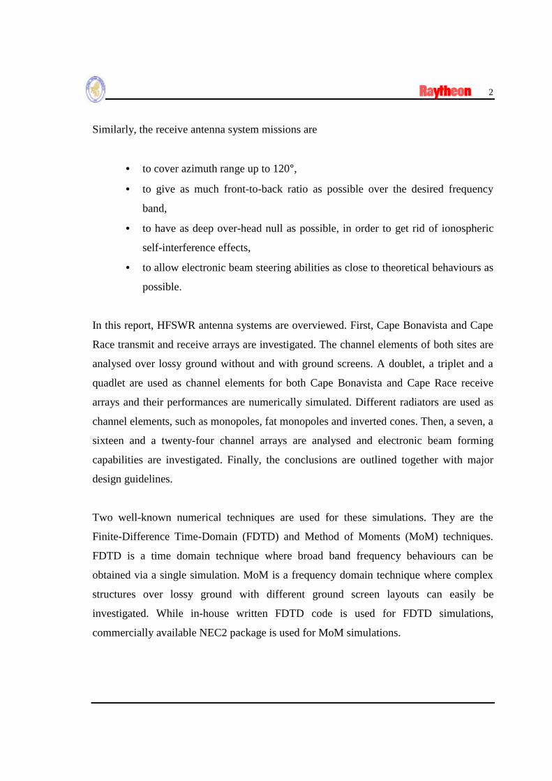
0 dB = 1.0dBi
Channels with Fat Monopoles
3.5MHz4.5MHz5.5MHz
Triplet
Fig. 3.29
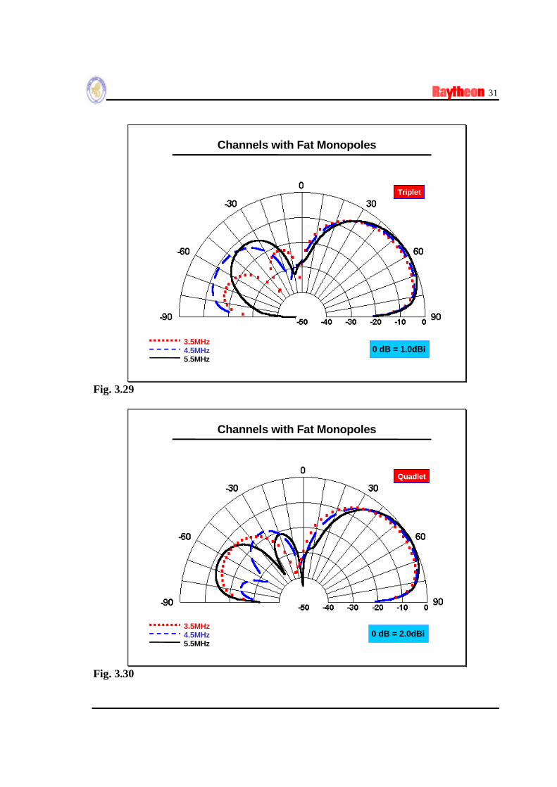
0 dB = 2.0dBi
Channels with Fat Monopoles
3.5MHz4.5MHz5.5MHz
Quadlet
Fig. 3.30

32
0 dB = -7.7dBi
Channels with Fat Monopoles
3.5MHz4.5MHz5.5MHz
Doublet
Fig. 3.31
0 dB = -7.0dBi
Channels with Fat Monopoles
3.5MHz4.5MHz5.5MHz
Triplet
Fig. 3.32

33
0 dB = -5.8dBi
Channels with Fat Monopoles
3.5MHz4.5MHz5.5MHz
Quadlet
Fig. 3.33

34
3.3 Crossed Monopoles
CODAR system [1] has been used in remote sensing of ocean currents. The system
operates at 25.4MHz and uses four quarter-wavelength vertical whips (as a unique array),
where they are symmetrically laid out on a circle with a radius of slightly less than
quarter-wavelength.
CODAR receive array is used both in beam forming and direction finding. The elements
of the array are fed in a way to maximise horizontal radiation in a desired direction. Since
there are four elements symmetrically laid out on a circle, the beam-width of the array is
nearly 90°. A special software package is used in conjunction with the array.
By phasing four-whips, 360° in azimuth may be steered. Examples related to azimuth
beam steering are given in Fig.s 3.34 to 3.36. The location of the array and whip
numbers, the phases of element feeding voltages are also mentioned in the figures.
It should be noted that, this array is effective when used in conjunction with the special
software package mentioned above. Otherwise, it is impossible to get azimuth
information with a beam-width of 90°. The package is used for the estimation of the
angle of arrival of a possible target signal by calculating the energy of beams formed for
a full circle of look-directions. Then, target signals arriving at certain angles appear as
peaks in beam energy versus angle plots.
Recently, a different design -based on CODAR array- has been introduced as an
alternative to linear arrays used in HFSWR. There, five 2m whips are grouped as
pentagon. The pentagon is elevated 20m on a pole, and two such poles are spaced 30m
apart (half-wavelength at 5MHz), so that ground screen is not essential.

35
This system is simulated via NEC package and the results are pictured in Fig.3.37. Here,
horizontal radiation patterns obtained by phasing each element in a way to maximise in a
desired direction is plotted.
Again, it should be noted that these antenna systems need to be used with powerful
direction estimation softwares
References
[1] D. E. Barrick & M. W. Evans , “Implementation of Coastal Current-Mapping HF RadarSystem” Progress Report No 1, NOAA Technical Memorandum, ERL-373-WPL-47, 1976

36
Fig.3.34
Fig.3.35
37
Fig.3.36
Fig.3.37

38
IV Receive Arrays
In a HFSWR based IMS system, the azimuth information is obtained by electronic beam
steering ability of the receive antenna system. Therefore, receive antenna system is
designed as an array of number of channels, which is adequate for the required beam-
width. Roughly speaking, the beam-width is inversely proportional with the antenna
length. The more narrower the beams the longer the arrays (i.e., higher number of
channels). For example, an array of nearly 1km length is required in order to obtain a 5°
beam-width at 3MHz frequency. If the channel spacing is quarter-wavelength (i.e., 25m
at 3MHz), then number of channels will be at least twenty.
In this section, arrays with different number of channels are investigated. First, seven-
channel arrays of both monopoles and fat monopoles are taken into account.
4.1 A seven-channel Array
In order to simulate array performances via NEC package effectively, number of wires
and segments is important. MoM technique is based on numerical solution of a set of
equations in a matrix form. The order of the matrix system is proportional with the
number of segments. As the number of segments increases linearly, the computation time
required for the matrix inversion increases exponentially. With a P-II based PC having
128MB RAM memory segments up to 2000 can be handled in a reasonable time. After
2000 segments it takes hours, even days to obtain NEC simulation results. In multi-
channel receive array modelling via NEC, the number of segments mostly depends on the
ground screen.
In order to get the array behaviour, while using reasonable amount of segments a seven-
channel array is taken into account. Since a monopole quadlet and fat monopole doublet
are used as the channel elements in Cape Bonavista and in Cape Race, respectively,
simulations are also carried out with these channel elements. A sixteen-element radial

39
ground system is used in both simulations. Radials of different vertical radiators are cut
and connected when intersected. The top view of the array, where quadlets are used as
channel elements, is pictured in Fig.4.1.
Numerical values such as antenna heights, wire and radial radii, inter-channel separations
are taken as mentioned in Sec.III.
Inter-array distances are taken as 31m and 33m for monopole and fat monopole arrays,
respectively.
Calculations are performed at two different frequencies, 3.5MHz and 4.5MHz.
The ground is assumed to be POOR.
In Fig.s 4.2 to 4.4 vertical as well as horizontal radiation characteristics –normalised to
0dB- are plotted and the gains with respect to isotropic radiator are mentioned in the
figure insets.

40
7×4 End-fire Array
Antenna height : 9.22mIntra-Quadlet dist. : 19mIntr-array distance : 31mNumber of radials : 16Radial lengths : 19m
Fig.4.1:
0 dB = 3.5dBi
7×4 End-fire Array
3.5MHz4.5MHz
0 dB = 11.2dBi
0 dB = 9.9dBi
POOR GroundPOOR Ground with Radials
3.5MHz
Fig.4.2:

41
3.5MHz 4.5MHz
0 dB = 9.9 dBi 0 dB = 11.2 dBi
FAT MONOPOLES
MONOPOLES
7 ELEMENT ARRAY WITH 16 RADIALS
Fig.4.3:
FAT MONOPOLES
MONOPOLES
7 ELEMENT ARRAY WITH 16 RADIALS
3.5MHz 4.5MHz
0 dB = 2.5 dBi 0 dB = 3.5 dBi
Fig.4.4:

42
4.2 A sixteen-channel Array
Simulations with seven-channel array show that horizontal radiation characteristics are
not much affected by the ground screen. But, array gain –with and without ground
screen- differs nearly 10dB.
HFSWR receive arrays will most probably be made up sixteen or twenty-four channels
depending on the requirements. Therefore, a sixteen-channel array is taken into account
in this section.
Again, the numerical values such as antenna heights, wire radius, inter-channel
separations are taken as mentioned in Sec.III.
Inter-array distances are taken as 31m and 33m for monopole and fat monopole arrays,
respectively.
Calculations are performed at 3.5MHz.
The ground is assumed to be POOR.
Suitable phasing the channels in the arrays simulates electronic beam steering
characteristics. The 3dB beam-width is approximately 8°.
In Fig.s 4.5 and 4.6 vertical as well as horizontal radiation characteristics –normalised to
0dB- are plotted and the gains with respect to isotropic radiator are mentioned in the
figure insets.

43
16 Element Array: Monopole versus Fat monopole
ϕ=-15° with Bore-sight3.5MHz
MonopoleFat monopole
Fig.4.5:
16 Element Array: Monopole versus Fat monopole
ϕ=30° with Bore-sight3.5MHz
MonopoleFat monopole
Fig.4.6:

44
4.3 A twenty-four channel Array
Finally, arrays at Cape Bonavista and Cape Race are simulated via NEC package.
Because of the segment limitations arrays are assumed to be located over POOR ground
without ground screen. Therefore, only horizontal beam forming is pictured in Fig.s 4.7
to 4.9.
Cable lengths from channels to the receiver are used as in Table 4.1.
Table 4.1:
Electrical cable lengths for 24 channels
CH # Cable [m] CH # Cable [m] CH # Cable [m] CH # Cable [m]
1 405.25 7 237.55 13 67.93 19 232.67
2 376.82 8 209.84 14 96.36 20 260.14
3 350.28 9 179.56 15 123.66 21 288.66
4 323.20 10 153.34 16 148.81 22 315.90
5 294.53 11 124.74 17 180.89 23 343.12
6 262.77 12 95.97 18 209.17 24 375.21
In an array of a large number of channels, it is of interest to know what happens if one or
more channels are turned off either intentionally or accidentally. Also, to reduce the cost
it is important to know how many and which channels can be omitted without
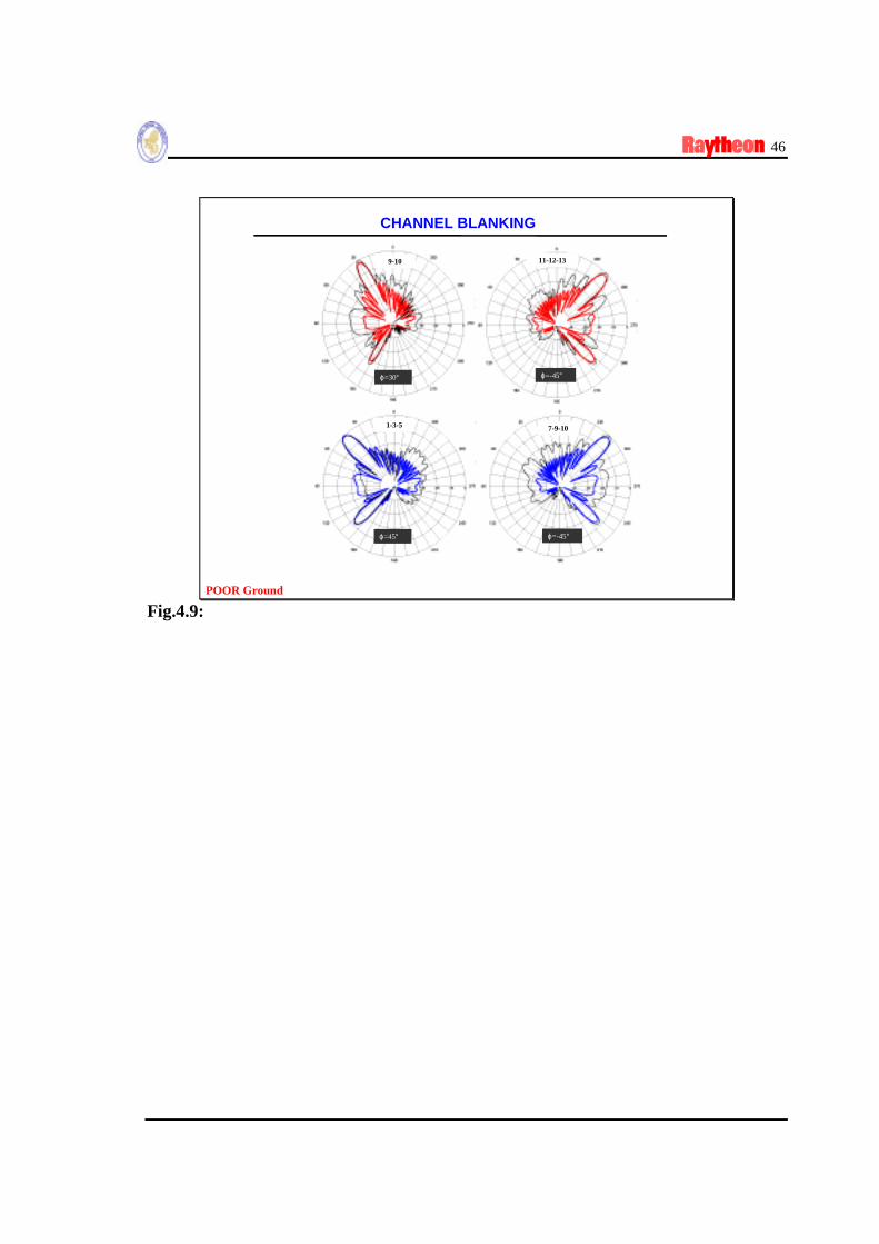
appreciably affecting the performance characteristics. Therefore, channel blanking is also
simulated in NEC calculations and the results are pictured in Fig.4.9. The channels are
numbered from 1 to 24 and the array is located along y-axis, where x-axis points the
array bore-sight. If top of this page is the array bore-sight, then the number of channels
increases from right to left. In Fig. 4.9, at top of each plot, the blanked channels are
mentioned.

45
ϕ=-60°
ϕ=0° ϕ=15° ϕ=-30°
ϕ=55°ϕ=-45°
CAPE RACE 24-ELEMENT FAT MONOPOLES
POOR Ground
Fig.4.7:
CAPE BON. 24-ELEMENT QUADLET ARRAY
ϕ=-60°
ϕ=0° ϕ=15° ϕ=-30°
ϕ=55°ϕ=-45°
POOR Ground
Fig.4.8:
46
CHANNEL BLANKING
POOR Ground
ϕ=30° ϕ=-45°
9-10 11-12-13
ϕ=45° ϕ=-45°
1-3-5 7-9-10
Fig.4.9:
47
V Ground Screen Design
A PEC surface has ideal 0Ω surface impedance. A quarter-wavelength vertical radiator
over PEC surface acts as a half-wavelength element in free-space. Therefore, its vertical
radiation pattern has a maximum towards horizontal. This is the design goal for an
HFSWR antenna element.
A lossy ground with ground parameters σg and εg has surface impedance, which can be
calculated via
2/1
0
2/1
00 1
+
+
+
=gggg
s i
i
i
iZ
ωεσωε
ωεσωε
η Ω= 3770η (5.1)
where ω=2πf is the radian frequency and η0 is the free space impedance. The surface
impedance of the POOR ground (i.e., the ground with σg=0.003 S/m and εg =4.0) is
around 150Ω at 2MHz, increases exponentially with the frequency and reaches to 300Ω
at 10MHz. But, the surface impedance of the ocean (i.e., when σg=5.0 S/m and εg =80.0)
is in between 5Ω-10Ω in the same frequency region. Therefore, ocean surface may easily
be assumed as a PEC surface at HFSWR operating frequencies.
The difference between erecting the antennas over POOR ground or PEC surface may
result in a reduction of gain by up to 15dB.
Beside this loss, there is also an extra near field propagation path loss because of the
POOR ground. Table 5.1 lists vertical electrical field strength and path loss at 1km away
from a 1kW vertical radiator.
48
It is clear from Table 5.1 that, at 1km distance; propagation loss over POOR ground may
be 10-15dB higher than the propagation loss over ocean surface.
Table 5.1:
Field strength and path loss values of a vertical radiator
with 1kW transmitter power at 1km distance
d=1km εg =15.0 f=3MHzConductivity
[S/m]Field Strength
[dBµV/m]Path Loss
[dB]0.0001 95.2 56.30.001 96.6 55.00.01 106.4 45.10.1 109.3 42.21.0 109.5 42.05.0 109.5 42.0
Therefore, together with the reduction in antenna gain, there may be a total of 30dB
extra loss just because the antenna elements are erected over POOR ground.
In order to overcome this problem, the surface impedance of the Antenna Park must be
reduced to an acceptable level. This is accomplished by one of two ways:
• The antenna park may be selected at the edge of the shore so that ocean water
flows under the antenna elements, or
• Using ground screen may reduce the surface impedance of the Antenna Park.
The first choice depends on available antenna site. If not available, then, ground screen
shall be used to reduce surface impedance of the Antenna Park.
Using ground screen

49
• will stabilise radiator’s input impedance, hence increase the antenna gain
• will lower the antenna TOA, hence more energy shall be coupled to ocean
surface.
In practice, three different types of ground screens are available. They are radials,
horizontal wires and rectangular meshes, or combinations of the three basic types.
It is simple to evaluate the effects of ground screen via approximate analytical
approaches. The impedance of a horizontal wire screen can be given as
≈
a
ddiZscr ππ
µω2
ln2
(5.2)
where a is the wire length and d is the wire separation. The same equation may also be
used for a mesh type screen if the mesh sizes are equal (i.e., square mesh) and equal to d.
Using the ground screen with impedance Zscr over lossy ground with surface impedance
Zs will cause an equivalent surface impedance, which can be given as
sscr
sscreq ZZ
ZZZ
+×
= (5.3)
the parallel equivalent of the two impedances.
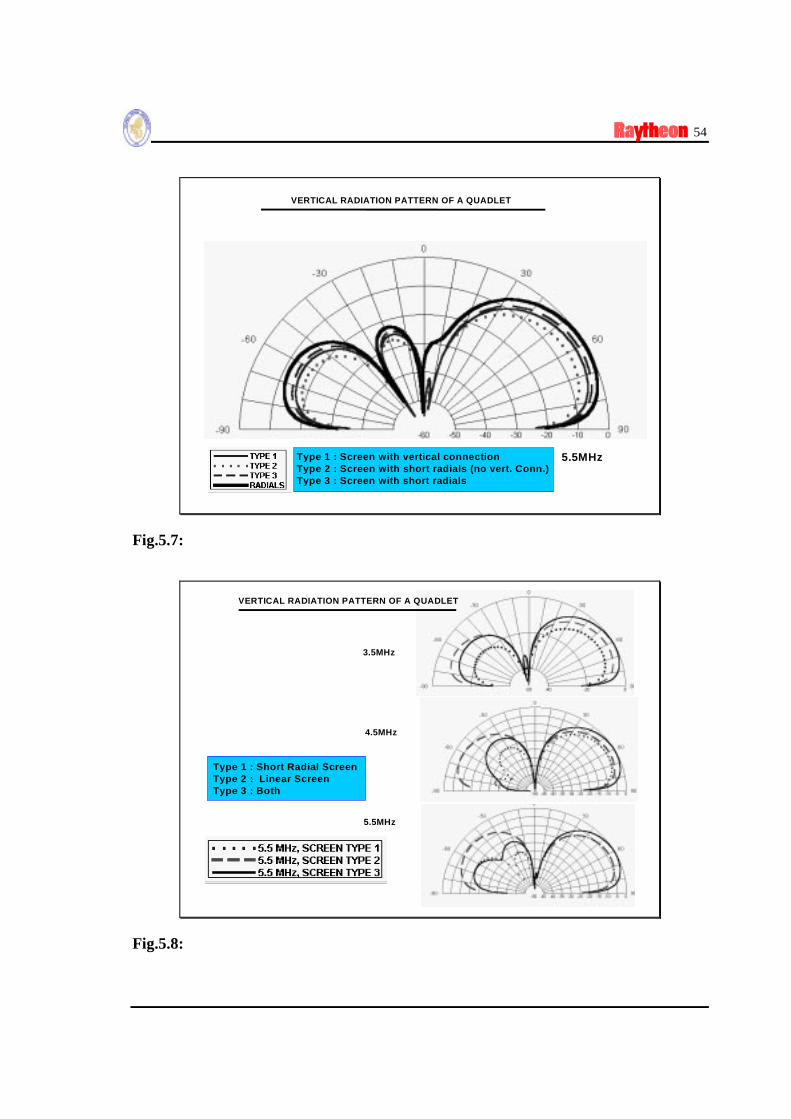
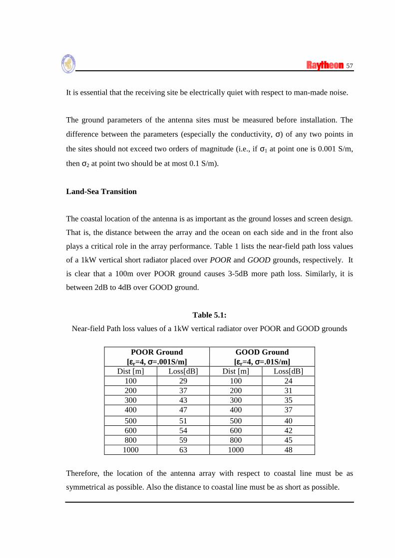
In this section, different ground screen layouts are taken into account as pictured in Fig.s
5.1 to 5.4. Their effects on radiation patterns and antenna gains are modelled via NEC
package and are plotted in Fig.s 5.5 to 5.8.

50
The NEC simulations are performed at 3.5MHz, 4.5MHz and 5.5MHz operating
frequencies.
The quadlet with monopoles mentioned in Sec.III are used with the same parameters.
Sixteen elements with 1m length are used as short radials. Quarter-wavelength horizontal
wires are used on each side of the antenna. The ground screen extends quarter-
wavelength behind and half-wavelength in front of the channel.
These results show the effect of ground screen for a single channel element. In HFSWR
arrays of multi-channel the effects may be more complicated.
Some general rules may be listed regarding to ground screen design:
• If the gain is crucial, then stabilising the elements input impedances is essential. It
may be done either by locating circular or rectangular PEC patches under each
vertical monopole element or using by radial wires.
• If lowering the TOA is crucial, then using horizontal wires that are perpendicular to
antenna bore-sight seems to be the most proper solution. In this case, horizontal wires
should extend at least quarter-wavelength at each side, half-wavelength at the back
and a wavelength in the front.
• If the over-head nulling is the most important requirement, keeping the antenna array
and ground screen depth (i.e., the size of the array along bore-sight) and avoiding
complex wiring in the ground screen layout are necessary. The more complex wire
connections the higher the diffractions and the lesser over-head nulling property.

51
ANTENNA SIMULATION WITH NEC
x
y
Fig.5.1:
ANTENNA SIMULATION WITH NEC
TYPE 1
Fig.5.2:

52
ANTENNA SIMULATION WITH NEC
TYPE 2
Fig.5.3:
ANTENNA SIMULATION WITH NEC
TYPE 3
Fig.5.4:
53
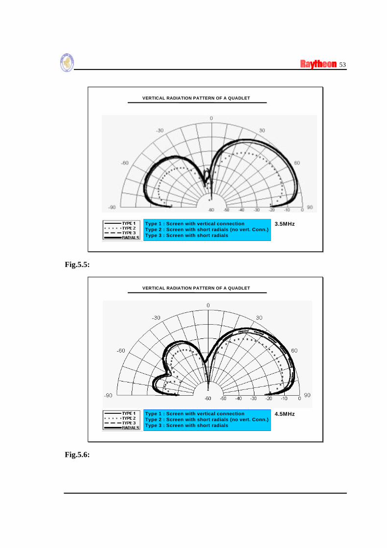
3.5MHz
VERTICAL RADIATION PATTERN OF A QUADLET
Type 1 : Screen with vertical connectionType 2 : Screen with short radials (no vert. Conn.)Type 3 : Screen with short radials
Fig.5.5:
4.5MHz
VERTICAL RADIATION PATTERN OF A QUADLET
Type 1 : Screen with vertical connectionType 2 : Screen with short radials (no vert. Conn.)Type 3 : Screen with short radials
Fig.5.6:
54
5.5MHz
VERTICAL RADIATION PATTERN OF A QUADLET
Type 1 : Screen with vertical connectionType 2 : Screen with short radials (no vert. Conn.)Type 3 : Screen with short radials
Fig.5.7:
3.5MHz
4.5MHz
5.5MHz
VERTICAL RADIATION PATTERN OF A QUADLET
Type 1 : Short Radial ScreenType 2 : Linear ScreenType 3 : Both
Fig.5.8:

55
VI Conclusions and Design Guidelines
In this report, HFSWR antenna arrays are investigated. Two powerful numerical
techniques are used to analyse
• Radiator elements such as monopoles and fat monopoles,
• Channel elements such as doublet, triplet and quadlets,
• Arrays with different number of channels,
• Ground screen designs.
General Design Guidelines
The design parameters of a HFSWR antenna system are
• Operating frequency bandwidth
• Maximum Directivity and Gain
• Maximum Front-to-back ratio
• Maximising over-head null
• Vertical and horizontal radiation patterns.
Good antenna system design will
• improve directivity, gain and surface wave coupling to reach longer ranges,
• enlarge azimuth coverage,
• increase front-to-back ratio to minimise interference originates sources behind
the array and back-located site interferences,
• provide deeper over-head null to reduce self-generated ionospheric interferences,
etc.

56
Antenna Site Requirements –Ideal:
Transmitter Site
The transmitter system requires a coastal shore site approximately 200m × 200m square
reasonable levelled (better than %1 grade) and not more than 10m above sea level.
The distance between the transmitter site and coastal line should be homogeneous and not
more than 100m.
The site characteristics must be suitable for the erection of transmitter antennas and
possible support tower, which may be up to 50m tall.
Receiver Site
The receiving system requires a coastal shore site approximately 1000m × 100m levelled
and not more than 10m above the mean sea level.
The long axis of this area must be parallel to the seashore and a line perpendicular to this
axis will define the receiving antenna array bore-sight. Land-sea transitions on each side
of the bore-sight should be similar and not include deep cavities and/or sharp edges.
The receiving antenna array must be separated from the transmitting antenna by at least
50m to avoid cross coupling. The transmit and receiving antenna systems must
horizontally null each other to increase cross-coupling strength.
The site characteristics must be suitable for the erection of primary receiving array, the
most probably a 16 channel doublets, nominally separated by 33m and not more than
15m tall, and the deployment of the receive equipment shelter.
57
It is essential that the receiving site be electrically quiet with respect to man-made noise.
The ground parameters of the antenna sites must be measured before installation. The
difference between the parameters (especially the conductivity, σ) of any two points in
the sites should not exceed two orders of magnitude (i.e., if σ1 at point one is 0.001 S/m,
then σ2 at point two should be at most 0.1 S/m).
Land-Sea Transition
The coastal location of the antenna is as important as the ground losses and screen design.
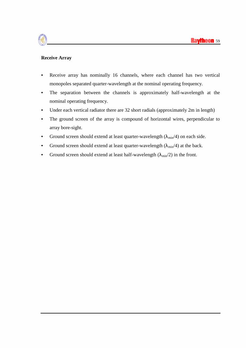
That is, the distance between the array and the ocean on each side and in the front also
plays a critical role in the array performance. Table 1 lists the near-field path loss values
of a 1kW vertical short radiator placed over POOR and GOOD grounds, respectively. It
is clear that a 100m over POOR ground causes 3-5dB more path loss. Similarly, it is
between 2dB to 4dB over GOOD ground.
Table 5.1:
Near-field Path loss values of a 1kW vertical radiator over POOR and GOOD grounds
POOR Ground[εr=4, σ=.001S/m]
GOOD Ground[εr=4, σ=.01S/m]
Dist [m] Loss[dB] Dist [m] Loss[dB]100 29 100 24200 37 200 31300 43 300 35400 47 400 37500 51 500 40600 54 600 42800 59 800 451000 63 1000 48
Therefore, the location of the antenna array with respect to coastal line must be as
symmetrical as possible. Also the distance to coastal line must be as short as possible.

58
The Antenna Channel
Typical channel for both transmit and receive array is pictured in Fig.1.
Figure 1: The top view of the HFSWR antenna channel
Transmit Array
• Transmit array has two vertical monopoles separated quarter-wavelength at the
nominal operating frequency.
• Under each vertical radiator there are 32 short radials (approximately 2m in length)
• The ground screen of the array is compound of horizontal wires, perpendicular to
array bore-sight.
• Ground screen should extend at least quarter-wavelength (λmin/2) on each side.
• Ground screen should extend at least quarter-wavelength (λmin/2) at the back.
• Ground screen should extend at least half-wavelength (λmin) in the front (if not
directly located at the coastal line).
59
Receive Array
• Receive array has nominally 16 channels, where each channel has two vertical
monopoles separated quarter-wavelength at the nominal operating frequency.
• The separation between the channels is approximately half-wavelength at the
nominal operating frequency.
• Under each vertical radiator there are 32 short radials (approximately 2m in length)
• The ground screen of the array is compound of horizontal wires, perpendicular to
array bore-sight.
• Ground screen should extend at least quarter-wavelength (λmin/4) on each side.
• Ground screen should extend at least quarter-wavelength (λmin/4) at the back.
• Ground screen should extend at least half-wavelength (λmin/2) in the front.

1
HFSWR RADAR ANTENNA ARRAYS
General Design Guidelines
The design parameters of a HFSWR antenna system are
• Operating frequency bandwidth
• Maximum Directivity and Gain
• Maximum Front-to-back ratio
• Maximising over-head null
• Vertical and horizontal radiation patterns.
Good antenna system design will
• improve directivity, gain and surface wave coupling to reach longer ranges,
• enlarge azimuth coverage,
• increase front-to-back ratio to minimise interference originates sources behind
the array and back-located site interferences,
• provide deeper over-head null to reduce self-generated ionospheric interferences,
etc.
HFSWR antenna systems are located on earth’s lossy ground, where the bore-sight points
the centre of azimuth coverage. The electrical parameters of the ground play a critical
role in antenna performance. Typical parameters for Good Land and Poor land are
εrg=15.0, σg=0.01 S/m and εrg=4.0, σg=0.003 S/m, respectively. On the other hand, ocean
parameters are εrg=80.0, σg=5.0 S/m. At HF frequencies the smooth ocean surface acts
almost as a perfectly electrical conductor (PEC). A vertical monopole with length l over a
2
PEC surface acts as a dipole with an equivalent length of 2l in free-space. Therefore, a
quarter-wavelength monopole over PEC acts as a half-wavelength dipole in free-space.
The angle between the horizontal plane and the vertical radiation maximum is called the
take-of-angle (TOA). Vertical monopoles over PEC surface have a 0° TOA. As the
surface loss increases TOA also increases.
A vertical monopole element has a donut radiation characteristic. That is, isotropic in
azimuth plane with horizontal maximum and vertical minimum radiation. However, when
placed over lossy ground the horizontal maximum tilts up to between 25° to 40° and the
antenna gain reduces by 10dB to 15dB, depending on the ground parameters.
Ground Screen Design
A PEC surface has ideal 0Ω surface impedance. A quarter-wavelength vertical radiator
over PEC surface acts as a half-wavelength element in free-space. Therefore its vertical
radiation pattern has a maximum towards horizontal. This is the design goal for an
HFSWR antenna element.
A lossy ground with the ground parameters σg and εg has surface impedance, which can
be calculated via
2/1
0
2/1
00 1
+
+
+
=gggg
s i
i
i
iZ
ωεσωε
ωεσωε
η Ω= 3770η (1)
where ω=2πf is the radian frequency and η0 is the free space impedance. The surface
impedance of the POOR ground (i.e., the ground with σg=0.003 S/m and εg =4.0) is
around 150Ω at 2MHz, increases exponentially with the frequency and reaches to 300Ω
at 10MHz. But, the surface impedance of the ocean (i.e., when σg=5.0 S/m and εg =80.0)

3
is in between 5Ω-10Ω in the same frequency region. Therefore, ocean surface may easily
be assumed as a PEC surface at HFSWR operating frequencies.
The difference between erecting the antennas over POOR ground or over the PEC surface
may result in a reduction of gain by up to 15dB.
Beside this loss, there is also an extra near field propagation path loss because of the
POOR ground. Table 1 lists vertical electrical field strength and path loss at 1km away
from a 1kW vertical radiator.
Table 1:
Field strength and path loss values of a vertical radiator
with 1kW transmitter power at 1km distance
d=1km εg =15.0 f=3MHzConductivity
[S/m]Field Strength
[dBµV/m]Path Loss
[dB]0.0001 95.2 56.30.001 96.6 55.00.01 106.4 45.10.1 109.3 42.21.0 109.5 42.05.0 109.5 42.0
It is clear from Table 1 that, at 1km distance; propagation loss over POOR ground may
be 10-15dB higher than the propagation loss over ocean surface.
Therefore, together with the reduction in antenna gain, there may be a total of 30dB
extra loss just because the antenna elements are erected over POOR ground.

4
In order to overcome this problem, the surface impedance of the Antenna Park must be
reduced to an acceptable level. This is accomplished by one of two ways:
• The antenna park may be selected at the edge of the shore so that ocean water
flows under the antenna elements, or
• Using a ground screen to reduce the surface impedance of the Antenna Park.
The first choice depends on available antenna site. If not available, then ground screen
shall be used to reduce surface impedance of the Antenna Park.
Using ground screen
• will stabilise radiator’s input impedance, hence increase the antenna gain
• will lower the antenna TOA, hence more energy shall be coupled to ocean
surface.
In practice, three different types of ground screens are available. They are radials,
horizontal wires and rectangular meshes, or combinations of the three basic types.
It is simple to evaluate the effects of ground screen via approximate analytical
approaches. The impedance of a horizontal wire screen is given by:
≈
a
ddiZscr ππ
µω2
ln2
(2)
where “a” is the wire length and “d” is the wire separation. The same equation may also
be used for a mesh type screen if the mesh sizes are equal (i.e., square mesh) and equal to
“d”.

5
Using the ground screen with impedance Zscr over lossy ground with surface impedance
Zs will cause an equivalent surface impedance, which is given by:
sscr
sscreq ZZ
ZZZ
+×
= (3)
the parallel equivalent of the two impedances.
Land-Sea Transition
The coastal location of the antenna is as important as the ground losses and screen design.
That is, the distance between the array and the ocean on each side and in the front also
plays a critical role in the array performance. Table 2 lists the near-field path loss values
of a 1kW vertical short radiator placed over POOR and GOOD grounds, respectively. It
is clear that a 100m over POOR ground causes 3-5dB more path loss. Similarly, it is
between 2dB to 4dB over GOOD ground.
Table 2:
Near-field Path loss values of a 1kW vertical radiator over POOR and GOOD grounds
POOR Ground[εr=4, σ=.001S/m]
GOOD Ground[εr=4, σ=.01S/m]
Dist [m] Loss[dB] Dist [m] Loss[dB]100 29 100 24200 37 200 31300 43 300 35400 47 400 37500 51 500 40600 54 600 42800 59 800 451000 63 1000 48
6
Therefore, the location of the antenna array with respect to coastal line must be as
symmetrical as possible. Also the distance to coastal line must be as short as possible.
Antenna Site Requirements –Ideal:
Transmitter Site
The transmitter system requires a coastal shore site approximately 200m × 200m square
reasonable levelled (better than %1 grade) and not more than 10m above sea level.
The distance between the transmitter site and coastal line should be homogeneous and not
more than 100m.
The site characteristics must be suitable for the erection of transmitter antennas and
possible support tower, which may be up to 50m tall.
Receiver Site
The receiving system requires a coastal shore site approximately 1000m × 100m levelled
and not more than 10m above the mean sea level.
The long axis of this area must be parallel to the seashore and a line perpendicular to this
axis will define the receiving antenna array bore-sight.
Land-sea transitions on each side of the bore-sight should be similar and not include deep
cavities and/or sharp edges.

7
The receiving antenna array must be separated from the transmitting antenna by at least
50m to avoid cross coupling. The transmit and receiving antenna systems must
horizontally null each other to increase cross-coupling strength.
The site characteristics must be suitable for the erection of primary receiving array, the
most probably a 16 channel doublets, nominally separated by 33m and not more than
15m tall, and the deployment of the receive equipment shelter.
It is essential that the receiving site be electrically quiet with respect to man-made noise.
The ground parameters of the antenna sites must be measured before installation. The
difference between the parameters (especially the conductivity, σ) of any two points in
the sites should not exceed two orders of magnitude (i.e., if σ1 at point one is 0.001 S/m,
then σ2 at point two should be at most 0.1 S/m).
The Antenna Channel
Typical channel for both transmit and receive array is pictured in Fig.1.
Figure 1: The top view of the HFSWR antenna channel
8
Transmit Array
• Transmit array has two vertical monopoles separated quarter-wavelength at the
nominal operating frequency.
• Under each vertical radiator there are 32 short radials (approximately 2m in length)
• The ground screen of the array is compound of horizontal wires, perpendicular to
array bore-sight.
• Ground screen should extend at least quarter-wavelength (λmin/2) on each side.
• Ground screen should extend at least quarter-wavelength (λmin/2) at the back.
• Ground screen should extend at least half-wavelength (λmin) in the front (if not
directly located at the coastal line).
Receive Array
• Receive array has nominally 16 channels, where each channel has two vertical
monopoles separated quarter-wavelength at the nominal operating frequency.
• The separation between the channels is approximately half-wavelength at the
nominal operating frequency.
• Under each vertical radiator there are 32 short radials (approximately 2m in length)
• The ground screen of the array is compound of horizontal wires, perpendicular to
array bore-sight.
• Ground screen should extend at least quarter-wavelength (λmin/4) on each side.
• Ground screen should extend at least quarter-wavelength (λmin/4) at the back.
• Ground screen should extend at least half-wavelength (λmin/2) in the front.
Recommended