gnm: an R Package for Generalized Nonlinear
Models
Heather Turner
Department of StatisticsUniversity of Warwick, UK
Heather Turner (University of Warwick) gnm Package WU April 2008 1 / 47
Overview
What is a generalized nonlinear model (GNM)?
How does gnm fit GNMs?
What are the key functions in gnm?
Using gnm to fit a ‘standard’ GNM
Using gnm to fit a custom GNM
Heather Turner (University of Warwick) gnm Package WU April 2008 2 / 47

Generalized Linear Models
A GLM is made up of a linear predictor
η = β0 + β1x1 + ...+ βpxp
and two functionsI a link function that describes how the mean, E(Y ) = µ,
depends on the linear predictor
g(µ) = η
I a variance function that describes how the variance, V ar(Y )depends on the mean
V ar(Y ) = φV (µ)
where the dispersion parameter φ is a constant
Heather Turner (University of Warwick) gnm Package WU April 2008 3 / 47

Generalized Nonlinear Models
A generalized nonlinear model (GNM) is the same as aGLM except that we have
g(µ) = η(x; β)
where η(x; β) is nonlinear in the parameters β.
Thus a GNM may also be considered as an extension of anonlinear least squares model in which the variance of theresponse is allowed to depend on the mean.
There a several models in the literature that fit within thisframework.
Heather Turner (University of Warwick) gnm Package WU April 2008 4 / 47

Models for Contingency Tables
Goodman’s row-column association model for 2 way tables
log µij = αi + βj + γiδj
UNIDIFF model for 3 way tables
log µijk = αik + βjk + γkδij
Diagonal reference model for square tables
µij = wγi + (1− w)γj
These are specific examples with multiplicative terms
Heather Turner (University of Warwick) gnm Package WU April 2008 5 / 47

More Models with Multiplicative Terms
AMMI model for Gaussian crop yields
µij = αi + βj + σ1γ1iδ1j + σ2γ2iδ2j
Lee-Carter model for (Quasi-)Poisson mortality rates
log(µay/eay) = αa + βaγy,
Rasch-type model for Binomial voting data
logit(µrm) = αr + βrγm
Stereotype model for ordered Multinomial data
log µic = β0c + γc(β1x1i + β2x2i)
Heather Turner (University of Warwick) gnm Package WU April 2008 6 / 47

Other Models
Although most standard applications have multiplicative terms,there is no restriction to such models.
For example, gnm may be used to exponential decay models ofthe form
µ = α + exp(β1 + γ1x) + exp(β2 + γ2x)
which nls is unable to fit.
Heather Turner (University of Warwick) gnm Package WU April 2008 7 / 47

The gnm Function
Models are specified via symbolic formulaeI functions of class "nonlin" to specify nonlinear terms
Single IWLS algorithm for all modelsI works with over-parameterized models
Patterned after glmI similar arguments, returned objects, methods, etc
Heather Turner (University of Warwick) gnm Package WU April 2008 8 / 47

Model Specification
Linear terms in the model may be specified in the usual way, e.g.y ∼ a + b + a:b
Nonlinear terms must be specified using functions of class"nonlin"
I specify structure of term, possible also labels & starting valuesI provided functions: Exp, Inv, Mult, MultHomog, DrefI custom functions
Heather Turner (University of Warwick) gnm Package WU April 2008 9 / 47

Nesting and Instances
Nonlin terms may be nested, e.g. for a UNIDIFF model:
log µijk = αik + βjk + exp(γk)δij
the exponentiated multiplier is specified as
Mult(Exp(C), A:B)
Multiple instances e.g. in Goodman’s RC(2) model:
log µrc = αr + βc + γrδc + θrφc
may be specified using the instances function:
instances(Mult(A, B), 2)
Heather Turner (University of Warwick) gnm Package WU April 2008 10 / 47
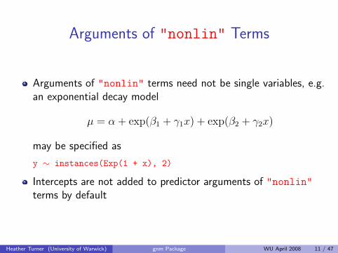
Arguments of "nonlin" Terms
Arguments of "nonlin" terms need not be single variables, e.g.an exponential decay model
µ = α + exp(β1 + γ1x) + exp(β2 + γ2x)
may be specified as
y ∼ instances(Exp(1 + x), 2)
Intercepts are not added to predictor arguments of "nonlin"terms by default
Heather Turner (University of Warwick) gnm Package WU April 2008 11 / 47

Working with Over-Parameterised Models
gnm does not impose any identifiability constraints on thenonlinear parameters
I the same model can be represented by an infinite number ofparameterisations, e.g.
logµrc = αr + βc + γrδc
= αr + βc + (2γr)(0.5δc)
= αr + βc + γ′rδ
′c
I gnm will return one of these parameterisations, at random
Rules for constraining nonlinear parameters not required
Fitting algorithm must be able to handle singular matrices
Heather Turner (University of Warwick) gnm Package WU April 2008 12 / 47

Parameter Estimation
Wish to estimate the predictor
η = η(β)
which is nonlinear, so we have a local design matrix
X(β) =∂η
∂β
where X is not of full rank, due to over-parameterisation
Use maximum likelihood estimation: want to solve the likehoodscore equations
U(β) = ∇l(β) = 0
Heather Turner (University of Warwick) gnm Package WU April 2008 13 / 47

Fitting Algorithm
Use a two stage procedure:I one-parameter-at-a-time Newton method to update nonlinear
parametersI full Newton-Raphson to update all parameters but with the
Moore-Penrose pseudoinverse (XTWX)−
Starting values are obtained in two ways:
for the linear parameters use estimates from a glm fitfor the nonlinear parameters generate randomly
I parameterisation determined by the starting values of nonlinearparameters
Heather Turner (University of Warwick) gnm Package WU April 2008 14 / 47

Estimating Identifiable Parameter Combinations
Prior to fittingI using arguments constrain and constrainTo
After fittingI estimate simple contrasts using getContrastsI estimate linear combinations of parameters using se
Both getContrasts and se check estimability first
Heather Turner (University of Warwick) gnm Package WU April 2008 15 / 47

Example: Yaish Data
Study of social mobility by Yaish (1998, 2004)
3-way contingecny table classified by:
orig father’s social class (7 levels)dest son’s social class (7 levels)educ son’s education level (5 levels)
Heather Turner (University of Warwick) gnm Package WU April 2008 16 / 47

UNIDIFF Model
In a UNIDIFF model
log µijk = αik + βjk + exp(γk)δij
exp(γk) is the strength of association over dimension indexed byi and j.Fit to yaish data:> unidiff <- gnm(Freq ~ educ*orig + educ*dest
+ Mult(Exp(educ), orig:dest),ofInterest = "[.]educ",family = poisson,data = yaish, subset = (dest != 7))
Heather Turner (University of Warwick) gnm Package WU April 2008 17 / 47

Summary of Fitted UNIDIFF ModelCall:
gnm(formula = Freq ~ educ * orig + educ * dest + Mult(Exp(educ),
orig:dest), ofInterest = "[.]educ", family = poisson, data = yaish,
subset = (dest != 7))
Deviance Residuals:
Min 1Q Median 3Q Max
-3.0286 -0.6402 -0.1048 0.5813 2.7459
Coefficients of interest:
Estimate Std. Error z value Pr(>|z|)
Mult(Exp(.), orig:dest).educ1 -0.4531 NA NA NA
Mult(Exp(.), orig:dest).educ2 -0.6785 NA NA NA
Mult(Exp(.), orig:dest).educ3 -1.1965 NA NA NA
Mult(Exp(.), orig:dest).educ4 -1.4920 NA NA NA
Mult(Exp(.), orig:dest).educ5 -2.7026 NA NA NA
Std. Error is NA where coefficient has been constrained or is unidentified
Residual deviance: 200.33 on 116 degrees of freedom
AIC: 1140.4
Number of iterations: 48Heather Turner (University of Warwick) gnm Package WU April 2008 18 / 47
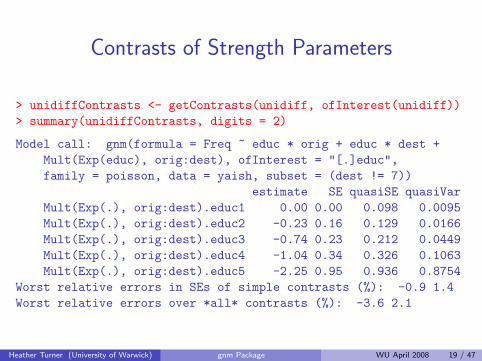
Contrasts of Strength Parameters
> unidiffContrasts <- getContrasts(unidiff, ofInterest(unidiff))> summary(unidiffContrasts, digits = 2)
Model call: gnm(formula = Freq ~ educ * orig + educ * dest +Mult(Exp(educ), orig:dest), ofInterest = "[.]educ",family = poisson, data = yaish, subset = (dest != 7))
estimate SE quasiSE quasiVarMult(Exp(.), orig:dest).educ1 0.00 0.00 0.098 0.0095Mult(Exp(.), orig:dest).educ2 -0.23 0.16 0.129 0.0166Mult(Exp(.), orig:dest).educ3 -0.74 0.23 0.212 0.0449Mult(Exp(.), orig:dest).educ4 -1.04 0.34 0.326 0.1063Mult(Exp(.), orig:dest).educ5 -2.25 0.95 0.936 0.8754
Worst relative errors in SEs of simple contrasts (%): -0.9 1.4Worst relative errors over *all* contrasts (%): -3.6 2.1
Heather Turner (University of Warwick) gnm Package WU April 2008 19 / 47

Contrasts Plotplot(unidiffContrasts, xlab = "Education Level", levelNames = 1:5)
1 2 3 4 5
−4
−3
−2
−1
0
Education level
estim
ate
●
●
●
●
●
Heather Turner (University of Warwick) gnm Package WU April 2008 20 / 47

Profiling
unidiff2 <- update(unidiff, constrain = "[.]educ1")prof <- profile(unidiff2, ofInterest(unidiff2), trace = TRUE)plot(prof)
−0.6 −0.2 0.2
−2
−1
0
1
2
3
Mult(Exp(.), orig:dest).educ2
z
−1.5 −1.0 −0.5 0.0
−2
−1
0
1
2
3
Mult(Exp(.), orig:dest).educ3
z
−2.5 −1.5 −0.5
−2
−1
0
1
2
3
Mult(Exp(.), orig:dest).educ4
z
−8 −6 −4 −2 0
−1
0
1
2
Mult(Exp(.), orig:dest).educ5
z
Heather Turner (University of Warwick) gnm Package WU April 2008 21 / 47

Profile Confidence Intervals
> conf <- confint(prof)> print(conf, digits = 2)
2.5 % 97.5 %Mult(Exp(.), orig:dest).educ1 NA NAMult(Exp(.), orig:dest).educ2 -0.6 0.1Mult(Exp(.), orig:dest).educ3 -1.5 -0.2Mult(Exp(.), orig:dest).educ4 -2.6 -0.3Mult(Exp(.), orig:dest).educ5 -Inf -0.7
Heather Turner (University of Warwick) gnm Package WU April 2008 22 / 47

Example: Marriage Data
The Living in Ireland Surveys were conducted 1994-2001
For five 5-year cohorts of women born between 1950 and 1975we have the following data
I year of (first) marriageI year and month of birthI social classI highest level of education attainedI year highest level of education was attained
Heather Turner (University of Warwick) gnm Package WU April 2008 23 / 47

Discrete-time Hazard Models
For discrete-time the hazard of marriage occuring at time t isdefined as
h(t) = P (T = t|T ≥ t)
We can model the hazard using models of the form
logit(h(t|xit)) = α(ageit) + x′itβ
Heather Turner (University of Warwick) gnm Package WU April 2008 24 / 47
Episode-splitting
To estimate the discrete-time hazard model we generate anevent history for each observation
Pseudo observations are created at each time point from time 0up to marriage or censoring - this is known as episode-splitting
The parameters can then be estimated by logistic regression of amarriage indicator at each time point (married = 1, unmarried= 0)
Heather Turner (University of Warwick) gnm Package WU April 2008 25 / 47

Blossfeld and Huinink Model
Blossfeld and Huinink (Am. J. Sociol., 1991) propose thefollowing linear baseline
α(ageit) = c+ βl log(ageit − 15) + βr log(45− ageit)
I describes the nature of the time dependenceI fixes the support of the hazard to be 15 to 45 years
Heather Turner (University of Warwick) gnm Package WU April 2008 26 / 47

BH Model
●
●
●
●
●
●
●
●
●
●●●●
●
●
●
●
●
●
●
●
●
●
●●
●●●●●
10 20 30 40 50
0.00
0.04
0.08
Age (years)
Pro
babi
lity
of M
arria
ge
Heather Turner (University of Warwick) gnm Package WU April 2008 27 / 47
Nonlinear Discrete-time Hazard Model
An obvious extension of the BH model is to treat the endpointsas parameters
α(ageit) = c+ βl log(ageit − αl) + βr log(αr − ageit)
I nonlinearI can’t specify with standard "nonlin" functions
Heather Turner (University of Warwick) gnm Package WU April 2008 28 / 47

Variables and Predictors
A "nonlin" function creates a list of arguments for the internalfunction nonlinTerms
Nonlinear terms are considered as functions of variables andpredictors
βl log(ageit − αl) + βr log(αr − ageit)
Create "nonlin" function Bell with argument x, which returnsthe argumentspredictors = list(slope = 1, endpoint = 1),variables = list(substitute(x))
Heather Turner (University of Warwick) gnm Package WU April 2008 29 / 47

Term-specific Issues
Would like to use same function for both “log-excess” terms, soadd argumentside = "left"
Need to constrain endpoints to avoid undefined log values, sodefineconstraint <- ifelse(side == "right",
max(x) + 1e-5, min(x) - 1e-5)
Heather Turner (University of Warwick) gnm Package WU April 2008 30 / 47

Term
The term argument of nonlinTerms takes labels for thepredictors and variables and returns a deparsed expression of theterm:term = function(predLabels, varLabels) {
paste(predLabels[1], " * log("," -"[side == "right"], varLabels[1], " + "," -"[side == "left"], constraint," + exp(", predLabels[2], "))")
}
Heather Turner (University of Warwick) gnm Package WU April 2008 31 / 47

Parameter Labels
Default parameter labels are taken from the predictor names,here slope and endpoint
To make parameter labels unique, save call to Bell:call <- sys.call()
and specify call argument to nonlinTerms
call = as.expression(call)match = c(0, 0)
Heather Turner (University of Warwick) gnm Package WU April 2008 32 / 47

Complete Function
Bell <- function(x, side = "left"){call <- sys.call()constraint <- ifelse(side == "right",
max(x) + 1e-5, min(x) - 1e-5)list(predictors = list(slope = 1, endpoint = 1),
variables = list(substitute(x)),term = function(predLabels, varLabels) {
paste(predLabels[1], " * log("," -"[side == "right"], varLabels[1], " + "," -"[side == "left"], constraint," + exp(", predLabels[2], "))")
},call = as.expression(call),match = c(0, 0))
}class(Bell) <- "nonlin"
Heather Turner (University of Warwick) gnm Package WU April 2008 33 / 47

Summary of Extended ModelCall:
gnm(formula = marriages/lives ~ Bell(age, side = "left") + Bell(age,
side = "right"), family = binomial, data = fulldata, weights = lives,
start = c(-20, 3, 0, 3, 0))
Deviance Residuals:
Min 1Q Median 3Q Max
-0.8098 -0.4441 -0.3224 -0.1528 4.0483
Coefficients:
Estimate Std. Error z value Pr(>|z|)
(Intercept) -118.5395 NA NA NA
Bell(age, side = "left")slope 3.6928 NA NA NA
Bell(age, side = "left")endpoint -0.1432 NA NA NA
Bell(age, side = "right")slope 24.8623 NA NA NA
Bell(age, side = "right")endpoint 4.0247 NA NA NA
Std. Error is NA where coefficient has been constrained or is unidentified
Residual deviance: 12553 on 31004 degrees of freedom
AIC: 12748
Number of iterations: 76Heather Turner (University of Warwick) gnm Package WU April 2008 34 / 47

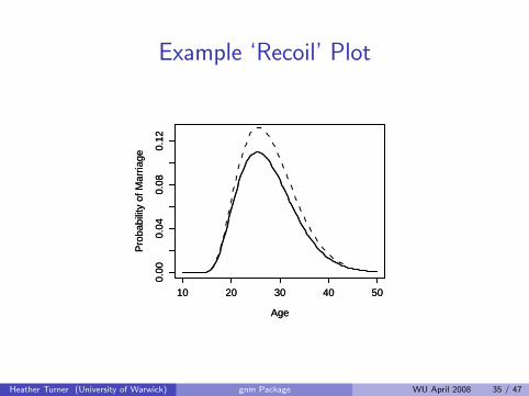
Example ‘Recoil’ Plot
10 20 30 40 50
0.00
0.04
0.08
0.12
Age
Pro
babi
lity
of M
arria
ge
Heather Turner (University of Warwick) gnm Package WU April 2008 35 / 47
Example ‘Recoil’ Plot
10 20 30 40 50
0.00
0.04
0.08
0.12
Age
Pro
babi
lity
of M
arria
ge
10 20 30 40 50
0.00
0.04
0.08
0.12
Age
Pro
babi
lity
of M
arria
ge
Heather Turner (University of Warwick) gnm Package WU April 2008 35 / 47
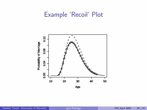
Example ‘Recoil’ Plot
10 20 30 40 50
0.00
0.04
0.08
0.12
Age
Pro
babi
lity
of M
arria
ge
10 20 30 40 50
0.00
0.04
0.08
0.12
Age
Pro
babi
lity
of M
arria
ge
10 20 30 40 50
0.00
0.04
0.08
0.12
Age
Pro
babi
lity
of M
arria
ge
●
●
●
●
●
●
●
●●
●●●
●
●
●
●
●
●
●
●●
●●
●●
●●●●
Heather Turner (University of Warwick) gnm Package WU April 2008 35 / 47

Re-parameterization
The problem with aliasing can be overcome by re-parameterizingthe model:
α(ageit) = γ − δ{
(ν − αl) log
(ν − αl
ageit − αl
)}+ δ
{(αr − ν) log
(αr − ν
αr − ageit
)}A new nonlin function, Surge, is need to specify this term
Heather Turner (University of Warwick) gnm Package WU April 2008 36 / 47
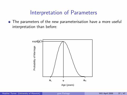
Interpretation of Parameters
The parameters of the new parameterisation have a more usefulinterpretation than before:
Age (years)
Pro
babi
lity
of M
arria
ge
ααL νν ααR
expit((γγ))
Heather Turner (University of Warwick) gnm Package WU April 2008 37 / 47

Recoil Plots for Reparameterised Model
x
pred
(x)
●●●●●
●
●
●
●
●
●●
●●●●
●
●
●
●
●●
●●
●●
●●●●●●●●●●●●
γγ−2.09 →→ −1.95
0.00
0.05
0.10
0.15
x
pred
(x)
●●
●
●
●
●
●
●●
●●●●●●
●●
●●
●●
●●
●●
●●
●●
νν25.39 →→ 28
x
pred
(x)
●
●
●
●
●
●
●●
●●●●●●
●●
●●
●●
●●
●●
●●●●●●
δδ0.34 →→ 0.15
xpr
ed (
x)
●●●
●
●
●
●
●
●●●●●
●●
●●
●●
●●
●●
●●●●●●●●●●●●●
ααL
−0.14 →→ 0.035
10 20 30 40 50
x
pred
(x)
●●●●
●
●
●
●
●
●●●●●
●●
●●
●●
●●
●●
●●●●●●●●●●●●●
ααR
4.02 →→ 20
0.00
0.05
0.10
0.15
10 20 30 40 50
10:50
rep(
0, 4
1)
●
Original ModelPerturbed ModelRe−fitted Model
Age (years)
Pro
babi
lity
of M
arria
ge
Heather Turner (University of Warwick) gnm Package WU April 2008 38 / 47
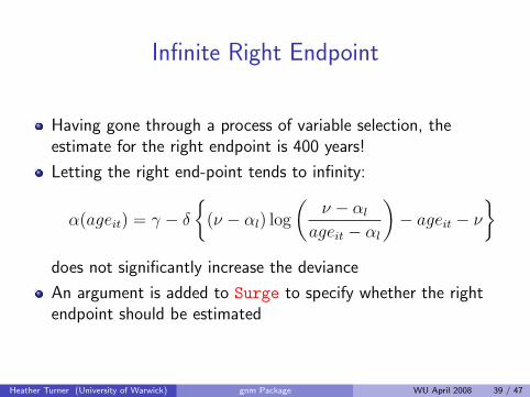
Infinite Right Endpoint
Having gone through a process of variable selection, theestimate for the right endpoint is 400 years!
Letting the right end-point tends to infinity:
α(ageit) = γ − δ{
(ν − αl) log
(ν − αl
ageit − αl
)− ageit − ν
}does not significantly increase the deviance
An argument is added to Surge to specify whether the rightendpoint should be estimated
Heather Turner (University of Warwick) gnm Package WU April 2008 39 / 47

Refining the Model
Checking the fit of the model over each covariate suggests somechanges in the predictors
I e.g. replacing the cohort factor by the nonlinear term
θ exp(λ(yrbi − 1950))
Residual analysis also suggests that both the scale and locationof hazard vary between individuals
Heather Turner (University of Warwick) gnm Package WU April 2008 40 / 47

Fit over Education Levels
●●
●
●
●
●
●
●
●
●
●
●
●●●
●●
●
●●
●
●●●●●
●
●●●
as.numeric(colnames(grp))
grpO
bs[i,
]
No attainment/primary(2366)
0.00
0.05
0.10
0.15
0.20
●●
●
●
●●
●
●
●
●
●
●
●●
●
●
●●
●
●
●●
●●●●
●
●●●
as.numeric(colnames(grp))
grpO
bs[i,
]
Lower secondary(7900)
●●
●
●
●
●●
●●
●
●
●
●
●
●
●
●●
●●●
●
●
●
●●
●
●●●
as.numeric(colnames(grp))
grpO
bs[i,
]
Upper secondary(11507)
15 20 25 30 35 40 45
●●●●●
●
●
●
●
●
●
●
●
●
●
●●
●●
●
●
●
●●●●●
●
●●
as.numeric(colnames(grp))
grpO
bs[i,
]
College(4829)
15 20 25 30 35 40 45
●●●●●●
●
●●
●
●●●
●
●
●
●
●
●
●
●
●
●
●
●
●
●
●
●●
as.numeric(colnames(grp))
grpO
bs[i,
]
University(4407)
as.numeric(colnames(grp))
grpO
bs[i,
] ● Observed
Model 13 (common peak)Model 14 (separate peaks)
Age (years)
Pro
port
ion
mar
ried
Heather Turner (University of Warwick) gnm Package WU April 2008 41 / 47

Linear Dependence of Peak Location
Quantifying the education level by the average equivalent yearsin education ed a linear dependence of peak location on age canbe incorporated as follows
α(xit) = γ − δ{
(ν0 + ν1edi − αl) log
(ν0 + ν1edi − αl
ageit − αl
)}+δ {ageit + ν0 + ν1edi}
An argument is added to Surge to specify the formula for thepeak location
Heather Turner (University of Warwick) gnm Package WU April 2008 42 / 47

Final Model
Coefficients:
(Intercept)
-1.59971836
Surge(age, peakX = ~ . + YrsEduc, right = Inf).peakX(Intercept)
14.42125516
Surge(age, peakX = ~ 1 + ., right = Inf).peakXYrsEduc
0.88430137
Surge(age, peakX = ~ 1 + YrsEduc, right = Inf)fallOff
0.46183848
Surge(age, peakX = ~ 1 + YrsEduc, right = Inf)leftAdj
0.16872262
Mult(., Exp(I(iyearb - 1950))).(Intercept)
-0.01991675
Mult(1, Exp(.)).I(iyearb - 1950)
0.19665983
InEduc
-1.46281777
PostEduc
-0.47859895
Heather Turner (University of Warwick) gnm Package WU April 2008 43 / 47

Hazard and Survival Curves
For women born in 1950
15 20 25 30 35 40 45
0.00
0.05
0.10
0.15
0.20
Age (years)
Pro
babi
lity
of m
arria
ge
10 20 30 40 50
0.0
0.2
0.4
0.6
0.8
1.0
Age (years)
Pro
port
ion
neve
r m
arrie
d
8.29.811.512.313.514.9
Deviance = 11847 Residual d.f. = 31000
Heather Turner (University of Warwick) gnm Package WU April 2008 44 / 47

Interpretation
α̂L = 13.86 and the deviance is significantly increased if this isconstrained to 15 years
Peak location varies from 21.32 years (no education) to 27.60years (university graduates)
Peak hazard varies from 0.17 (b. 1950) through 0.16 (b. 1960)to 0.07 (b. 1970)
Heather Turner (University of Warwick) gnm Package WU April 2008 45 / 47

References
More information about gnm can be found onwww.warwick.ac.uk/go/gnm
A comprehensive manual is distributed with the packagevignette("gnmOverview", package = "gnm")
A working paper on the marriage application is available atwww.warwick.ac.uk/go/crism/research/2007
Heather Turner (University of Warwick) gnm Package WU April 2008 46 / 47

Acknowledgements
The marriage data are from The Economic and Social ResearchInstitute Living in Ireland Survey Microdata File ( c©Economicand Social Research Institute).
We gratefully acknowledge Carmel Hannan for introducing us tothis application and providing background on the data.
Heather Turner (University of Warwick) gnm Package WU April 2008 47 / 47
Recommended