University of California, Berkeley
Department of Statistics
Genetic Algorithms and Poker Rule Induction
Wenjie Xu
Supervised by Professor David AldousSubmitted in fulfillment of the requirements for the degree of
honors in Statistics, May 2015

Abstract
This thesis is intended to be an experiment on Genetic Algorithms (GAs). The general algo-
rithm is applied to a specific dataset of poker hands. Its performance in detecting the rules of
poker games is then evaluated in different measures and conditions. Based on the performance
of the algorithm, further understanding of the data can be obtained.

Contents
Abstract 1
1 Introduction 2
2 Background Theory 4
2.1 Genetic Algorithms . . . . . . . . . . . . . . . . . . . . . . . . . . . . . . . . . . 4
2.2 Decision Trees . . . . . . . . . . . . . . . . . . . . . . . . . . . . . . . . . . . . . 5
2.3 Rule Induction . . . . . . . . . . . . . . . . . . . . . . . . . . . . . . . . . . . . 6
3 Data 8
4 Methodology 10
4.1 Sampling . . . . . . . . . . . . . . . . . . . . . . . . . . . . . . . . . . . . . . . . 10
4.2 Building Trees . . . . . . . . . . . . . . . . . . . . . . . . . . . . . . . . . . . . . 11
4.3 Genetic Algorithm . . . . . . . . . . . . . . . . . . . . . . . . . . . . . . . . . . 12
5 Findings 13
5.0.1 Results . . . . . . . . . . . . . . . . . . . . . . . . . . . . . . . . . . . . . 13
5.0.2 Discussion . . . . . . . . . . . . . . . . . . . . . . . . . . . . . . . . . . . 15
3

CONTENTS 1
6 Conclusion 17
Appendices 18
A 19
Bibliography 19
Chapter 1
Introduction
The idea of a learning machine that parallels the principles of natural evolution has been
around for more than 50 years. With the assistance of computer programming, this idea can
now transform into a set of techniques for optimization in the field of machine learning. It is
clear as to why an evolutionary algorithm that entails great randomness can give rise to good
solutions. Nevertheless, this idea has been utilized in many fields and proved to inspire powerful
methods in various settings.
The goal of this research is not to develop a predictive model using GAs from the given
data with optimized accuracy. Indeed, there are no rigorous mathematical theories that concern
the convergence of the results of a GA to the true maximum. The search for an optimized
solution is rather heuristic and a satisfactory approximation is rarely guaranteed. Moreover,
some assumptions of the other methods involved in this research can be too strong for the real
data to satisfy or deviant from the real situations. In other words, the methods are relatively
nave and may forgo important patterns in the true solutions due to some inherent weaknesses.
For example, although it is natural for humans to think in a way that relates and compares
different cards in a hand, it is fairly difficult for a machine to automatically develop such a
discerning eye.
With all this being said, the goal here is to obtain better understanding of GAs by exper-
imenting on them to build a predictive model on real data. Specifically, I would like to find
2
3
out about the factors that may affect the performance of a genetic algorithm, in searching for
a set of complex rules that dominate the assignment of class labels to poker hands. Through
experiments, it will be possible to make relevant comments on the factors and consequently,
propose ideas that may spawn better models.
The problem of poker rule induction is based on the set of simulated poker hands stored
in the UCI Machine Learning Repository. It is originally brought forward in a prediction
competition hosted by Kaggle.com. Ideally, the process of predicting labels is analogous to
inducing poker rules, as the essence of poker rules lies in the ability to recognize and compare
poker hands. Therefore, in order to tackle this problem, an algorithm based on the concepts
of GAs will be developed to train the computer to predict the class label for a given poker
hand as accurately as possible. No presumed knowledge of general poker rules is present in the
developing process. This algorithm is the major subject of all analysis involved in this research.
Chapter 2
Background Theory
2.1 Genetic Algorithms
Genetic algorithms are a general class of algorithms inspired by natural selection. They
have been widely applied to optimizing solutions for a great variety of problems, including
medicine, robotics, laser technology, etc. The method has rather simple and intuitive under-
lying concepts. It treats solutions to a specific problem as genes and simulates the process of
natural selection, with the hope of eventually getting better solutions. The main steps include
generating a random initial population of solutions, selecting a proportion of the population
with the best performance according to certain criteria, breeding a population of offspring from
the selected genes, treating the parents and children as the new initial population, and repeating
the process. Mutation is usually included to add to the randomness.
More formally, according to David A Coley in An Introduction to Genetic Algorithms for
Scientists and Engineers, a typical algorithm consists of the following:
1. A population of guesses of the solution to the problem;
2. A way of calculating how good or bad the individual solutions within the population are;
3. A method for mixing fragments of the better solutions to form new, on average even
4

2.2. Decision Trees 5
better solutions; and
4. A mutation operator to avoid permanent loss of diversity within the solutions.
To fulfill these tasks, individual solutions must be encoded in some manner so that they
resemble strings and can be manipulated like chromosomes. Then, three major operators are
employed: selection, crossover and mutation.
Selection refers to the process of weeding out the solutions with lower fitness and preserving
the ones with higher fitness, where fitness is calculated using some pre-specified formula to
correspond to the performance of a given solution.
The individuals, or solutions, that have survived the selection then proceed to the step
of crossover. One common method is to choose pairs of individuals promoted by the selection
operator, randomly choose a single cutting point within the strings, and swap all the information
to the right of this point between the two individuals.
Mutation is used to randomly change the value of single elements within individual strings.
It typically occurs at very low rates.
2.2 Decision Trees
Decision trees are a method of classifying observations. Since we are interested in dis-
covering the rules of poker games, which is equivalent to classifying poker hands according to
an ordinal set of pre-specified attributes, decision trees can be treated as individual solutions.
There are certainly other ways to represent rules. Decision trees are one of the simpler classi-
fying methods. More importantly, tree structures are suitable for applying GAs. They can be
easily encoded into strings of operations, with connected nodes and leaves.
In general, the process of growing trees include two steps:
1. Dividing the predictor space, the set of possible values for each predictor X1,X2,...,Xp
into J distinct and non-overlapping regions R1,R2,...,Rj;
6 Chapter 2. Background Theory
2. For every observation that falls into the jth region, making the same prediction, which is
the majority class of the response values for the training observations in that region.
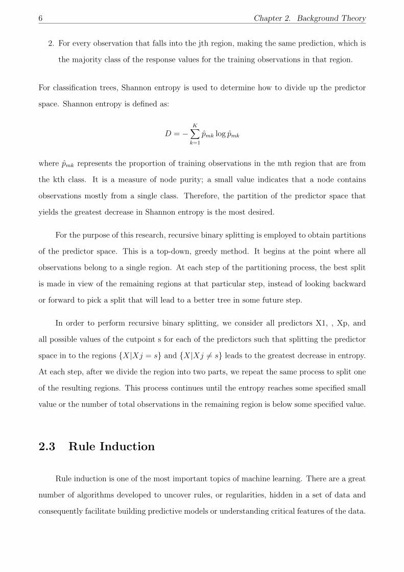
For classification trees, Shannon entropy is used to determine how to divide up the predictor
space. Shannon entropy is defined as:
D = −K∑k=1
p̂mk log p̂mk
where p̂mk represents the proportion of training observations in the mth region that are from
the kth class. It is a measure of node purity; a small value indicates that a node contains
observations mostly from a single class. Therefore, the partition of the predictor space that
yields the greatest decrease in Shannon entropy is the most desired.
For the purpose of this research, recursive binary splitting is employed to obtain partitions
of the predictor space. This is a top-down, greedy method. It begins at the point where all
observations belong to a single region. At each step of the partitioning process, the best split
is made in view of the remaining regions at that particular step, instead of looking backward
or forward to pick a split that will lead to a better tree in some future step.
In order to perform recursive binary splitting, we consider all predictors X1, , Xp, and
all possible values of the cutpoint s for each of the predictors such that splitting the predictor
space in to the regions {X|Xj = s} and {X|Xj 6= s} leads to the greatest decrease in entropy.
At each step, after we divide the region into two parts, we repeat the same process to split one
of the resulting regions. This process continues until the entropy reaches some specified small
value or the number of total observations in the remaining region is below some specified value.
2.3 Rule Induction
Rule induction is one of the most important topics of machine learning. There are a great
number of algorithms developed to uncover rules, or regularities, hidden in a set of data and
consequently facilitate building predictive models or understanding critical features of the data.

2.3. Rule Induction 7
Rules usually take the form:
X1 ∧X2 ∧ ... ∧XN ⇒ Y
The X’s and Y are logical events. As mentioned in the previous section, it is sensible to use
decision trees to represent rules. Here, the genetic algorithm based on decision trees is used to
search for rules hidden in the data set of poker hands.
Data from which rules are induced are usually presented in a table, where each case consists
of a number of attribute-value pairs and a decision-label pair. In the scope of this research,
only supervised learning is involved. That is, each case in the training data includes a number
of features, or independent variables, as well as the corresponding class label, or the dependent
variable.
The ideal goal of a rule induction method is to induce a rule set R that is consistent (there
exists no case contradicting the rule) and complete (all attribute-value pairs are covered). Such
a set of rules is called discriminant. Certainly, there is always trade-off between these two
characteristics as they can hardly be achieved at the same time.
Chapter 3
Data
The training data come from the kaggle.com competition Poker Rule Induction. There
are 25,010 poker hands. Each hand consists of 5 cards with a given suit and rank, drawn from
a standard deck of 52. Therefore, there are 10 features and 1 label for each observation. Suits
and ranks are represented as ordinal categories. For example, S1 refers to the suit of the first
card in the hand and a corresponding value in the range of 1 to 4 represents hearts, spades,
diamonds, and clubs respectively. C1 refers to the rank of the first card in the hand and a
corresponding value in the range of 1 to 13 represents ace, 2, 3, , and king respectively. In
addition, each row in the training set has the accompanying class label for the poker hand it
comprises.
Poker hands are classified into the following 10 ordinal categories:
0: Nothing in hand; not a recognized poker hand
1: One pair; one pair of equal ranks within five cards
2: Tow pairs; two pairs of equal ranks within five cards
3: Three of a kind; three equal ranks within five cards
4: Strain; five cards, sequentially ranked with no gaps
5: Flush; five cards with the same suit
8

9
6: Full house; pair + different rank three of a kind
7: Four of a kind; four equal ranks within five cards
8: Straight flush; straight + flush
9: Royal flush; ace, king, queen, jack, ten + flush
A characteristic of the training data is that straight flush and royal flush hands are not
representative of the true domain because they have been over-sampled. The straight flush is
14.43 times more likely to occur in the training set, while the royal flush is 129.82 times more
likely. This adds to the difficulty of developing machine learning mechanisms.
Moreover, 0 is a dominant class in the data. About 60% of the observations are labeled
as 0. This indicates that a predictive function that constantly generates 0 will achieve an
accuracy of 0.6 approximately. The presence of dominant classes usually sets a standard for
the performance of models.

Chapter 4
Methodology
The algorithm is implemented with Python, with possible adjustments and improvements.
There are mainly three steps: sampling, building the initial trees, and applying a generic
algorithm. Each step involves important parameters that may affect the final performance of
the genetic algorithm.
First of all, the validation set method is used to evenly divide the data set into two parts,
a training set and a test set. The algorithm is applied to the training set and various results
are obtained. The test set is used to evaluate the results in the end.
4.1 Sampling
Since the initial population for GAs consists of random solutions, at the first step of our
algorithm, a number of random samples are drawn from the entire training set to build an initial
population of decision trees that serve as the guesses for rules. The sample size is determined
using a 5-fold cross-validation method. The randomness of the samples ensures the randomness
of the initial generation, which conforms to the concepts of GAs.
10
4.2. Building Trees 11
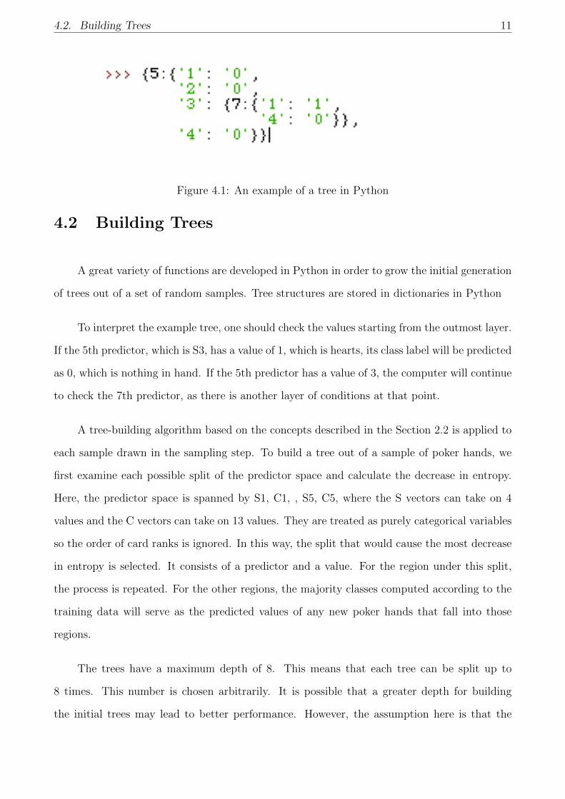
Figure 4.1: An example of a tree in Python
4.2 Building Trees
A great variety of functions are developed in Python in order to grow the initial generation
of trees out of a set of random samples. Tree structures are stored in dictionaries in Python
To interpret the example tree, one should check the values starting from the outmost layer.
If the 5th predictor, which is S3, has a value of 1, which is hearts, its class label will be predicted
as 0, which is nothing in hand. If the 5th predictor has a value of 3, the computer will continue
to check the 7th predictor, as there is another layer of conditions at that point.
A tree-building algorithm based on the concepts described in the Section 2.2 is applied to
each sample drawn in the sampling step. To build a tree out of a sample of poker hands, we
first examine each possible split of the predictor space and calculate the decrease in entropy.
Here, the predictor space is spanned by S1, C1, , S5, C5, where the S vectors can take on 4
values and the C vectors can take on 13 values. They are treated as purely categorical variables
so the order of card ranks is ignored. In this way, the split that would cause the most decrease
in entropy is selected. It consists of a predictor and a value. For the region under this split,
the process is repeated. For the other regions, the majority classes computed according to the
training data will serve as the predicted values of any new poker hands that fall into those
regions.
The trees have a maximum depth of 8. This means that each tree can be split up to
8 times. This number is chosen arbitrarily. It is possible that a greater depth for building
the initial trees may lead to better performance. However, the assumption here is that the
12 Chapter 4. Methodology
maximum depth of the first generation has no significant effect on the performance of the final
generation as long as the number of generation is large enough.
4.3 Genetic Algorithm
Given a population of trees grown in the previous section, predictions can be made for the
held-out test set and a fitness value can be obtained, since the test set is already labeled. Two
measure of fitness are concerned: sum of squared errors (SSE) and accuracy. SSE is used to
select the best performing individuals in each generation to survive.
Half of the trees in the initial population with higher fitness are selected. Then, the selected
trees are randomly and evenly assigned to two groups. Each tree from group A is paired up
with a tree from group B. For each pair, a random depth is generated and the branches of the
two trees at that depth are exchanged. This process corresponds to the basics of crossover in
GAs. The parent trees and the newly generated trees with exchanged branches form a new
generation with the same size as the initial one.
This procedure is repeated for a number of times, which is the number of generations, an
important parameter of the algorithm. Intuitively, more generations will lead to better results.
However, such intuition needs not to be true and it always remains a difficult task to find
out the optimal number of generations. For the purpose of this research, different generation
numbers will be tested on the test set and the results will be compared. The fitness of a whole
generation is represented by the highest fitness of the trees in it. To compare the performance
of different numbers of generations, it is sufficient to compare the fitness of the last generation
of each set.

Chapter 5
Findings
5.0.1 Results
Since fitness is calculated by testing the algorithm on the held-out test set, the evaluation
of the algorithm is mainly based on its performance on that test set. The parameters to our
interest are the sample size, the number of samples, and the number of generations. Their
mutual independence is assumed to hold so that each parameter can be examined separately.
To find out about a parameters effects, the other two are fixed at some arbitrary value.
For 100 generations of trees, each consisting of 100 trees, the sample sizes of 1000, 3000,
5000, and 7000 are experimented with. The resulting average SSE and accuracy of 10 experi-
ments are recorded in table 5.1. As the number of generations and population size are relatively
small, there are no significant trends or patterns in the relationship of sample size versus fit-
ness. Among the four sizes, the size of 1000 leads to the least SSE and the highest accuracy on
average.
For 100 generations of trees, with an initial sample of 1000 poker hands, the population
size of 100, 200, 300, 400, and 500 are experimented with. The resulting average SSE and
accuracy of 10 experiments are recorded in table 5.2. The population size of 400 leads to the
smallest SSE and the highest accuracy on average. There appears to be a positive correlation
between the population size and average accuracy. It is reasonable to suggest that a larger initial
13

14 Chapter 5. Findings
Sample Size SSE Accuracy
1000 10136.8 0.470790
3000 10270.1 0.47430
5000 10862.3 0.464740
7000 10460.6 0.472390
Table 5.1: Varying sample size
population may lead to more variation in the initial population and thus, higher probability
for the generations to converge to a better one.
Population Size SSE Accuracy
200 10317.3 0.471340
300 9951.4 0.471340
400 9526.6 0.475470
500 9719.2 0.46910
Table 5.2: Varying tree population size
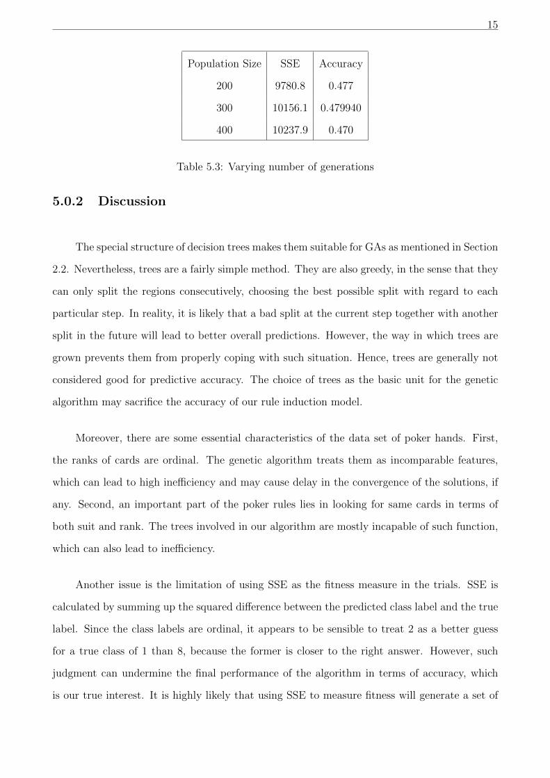
For a population size of 400 and a sample size of 1000, the number of generations of
200, 300, and 400 are experimented with. The resulting average SSE and accuracy of 10
experiments are recorded in table 5.3. SSE and accuracy do not agree in this case. The
population size of 200 leads to the least average SSE and 300 leads to the highest average
accuracy. By setting tree population size and sample size to be the best performing values from
the previous experiments and varying only the number of generation, no apparent improvements
in performance is achieved.
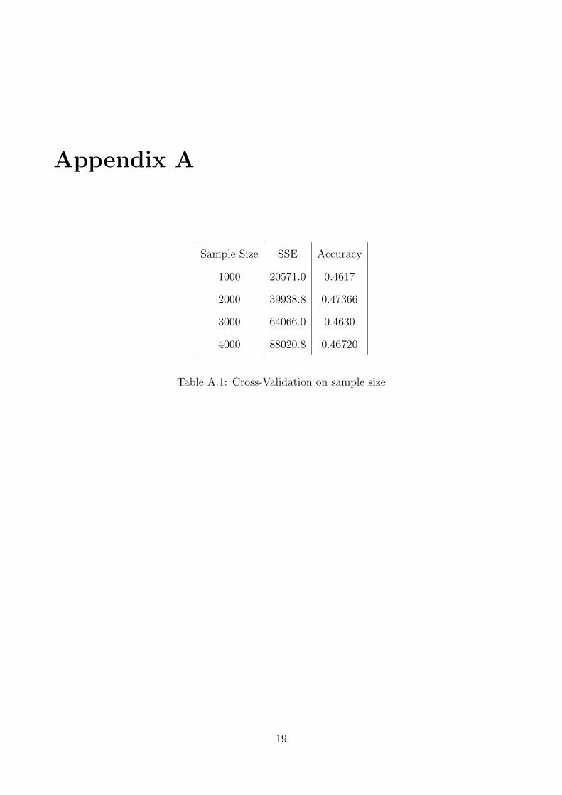
Doing 5-fold cross validation on the sample size gives similar results as the test set method.
Given a relatively small number of generations and population size, sample size does not ap-
pear to affect the algorithm significantly. The results of cross validation can be found in the
Appendix.
15
Population Size SSE Accuracy
200 9780.8 0.477
300 10156.1 0.479940
400 10237.9 0.470
Table 5.3: Varying number of generations
5.0.2 Discussion
The special structure of decision trees makes them suitable for GAs as mentioned in Section
2.2. Nevertheless, trees are a fairly simple method. They are also greedy, in the sense that they
can only split the regions consecutively, choosing the best possible split with regard to each
particular step. In reality, it is likely that a bad split at the current step together with another
split in the future will lead to better overall predictions. However, the way in which trees are
grown prevents them from properly coping with such situation. Hence, trees are generally not
considered good for predictive accuracy. The choice of trees as the basic unit for the genetic
algorithm may sacrifice the accuracy of our rule induction model.
Moreover, there are some essential characteristics of the data set of poker hands. First,
the ranks of cards are ordinal. The genetic algorithm treats them as incomparable features,
which can lead to high inefficiency and may cause delay in the convergence of the solutions, if
any. Second, an important part of the poker rules lies in looking for same cards in terms of
both suit and rank. The trees involved in our algorithm are mostly incapable of such function,
which can also lead to inefficiency.
Another issue is the limitation of using SSE as the fitness measure in the trials. SSE is
calculated by summing up the squared difference between the predicted class label and the true
label. Since the class labels are ordinal, it appears to be sensible to treat 2 as a better guess
for a true class of 1 than 8, because the former is closer to the right answer. However, such
judgment can undermine the final performance of the algorithm in terms of accuracy, which
is our true interest. It is highly likely that using SSE to measure fitness will generate a set of

16 Chapter 5. Findings
rules that give overall close predictions but few accurate predictions.
Chapter 6
Conclusion
The purpose of averaging the fitness values of the experiments is to look for signs of
convergence in the solutions. Occasionally, some solutions with impressive performance are
obtained. Nevertheless, the experiments exhibit high variance and the averaged performance
is not satisfactory for any value of the parameters. If the resulted rules with relatively high
performance on the chosen test set are used on a new, very different test set, it is very likely that
the performance will not be satisfactory. This reveals the nature of GAs as random searchers.
Parameters do not appear to play a crucial role in the performance of the algorithm. The
performance is subject to great uncertainty.
Due to the limitations and inefficiencies discussed earlier, the genetic algorithm may not be
a good model in terms of predictive accuracy. In general, the costs of the algorithm are relatively
high in light of the long time that it takes to operate and the low accuracy of the results. For
further improvements, mutation may be included in the process as it adds to the randomness
of the procedure and thus, helps avoid the trap of local maxima. Besides, more advanced trees
may be employed with operators that compare the magnitudes of different attributes. There
are certainly many other algorithms that would capture the regularities of the data better than
GAs and exhibit more rigorous properties. Due to the limit of this undergraduate research,
they are not examined here.
17

Appendices
18
Appendix A
Sample Size SSE Accuracy
1000 20571.0 0.4617
2000 39938.8 0.47366
3000 64066.0 0.4630
4000 88020.8 0.46720
Table A.1: Cross-Validation on sample size
19
Bibliography
Bache, K. & Lichman, M. (2013). UCI Machine Learning Repository. Irvine, CA: University
of California, School of Information and Computer Science.
Coley, David A. An Introduction to Genetic Algorithms for Scientists and Engineers. Singapore:
World Scientific, 1999. Print.
James, Gareth. An Introduction to Statistical Learning with Applications in R. Print.
Segaran, Toby. Programming Collective Intelligence: Building Smart Web 2.0 Applications.
Beijing: O’Reilly, 2007. Print.
20
Recommended