http://ijr.sagepub.com/Robotics Research
The International Journal of
http://ijr.sagepub.com/content/32/11/1275The online version of this article can be found at:
DOI: 10.1177/0278364913490533
2013 32: 1275 originally published online 15 July 2013The International Journal of Robotics ResearchMichael J. Gielniak, C. Karen Liu and Andrea L. Thomaz
Generating human-like motion for robots
Published by:
http://www.sagepublications.com
On behalf of:
Multimedia Archives
can be found at:The International Journal of Robotics ResearchAdditional services and information for
http://ijr.sagepub.com/cgi/alertsEmail Alerts:
http://ijr.sagepub.com/subscriptionsSubscriptions:
http://www.sagepub.com/journalsReprints.navReprints:
http://www.sagepub.com/journalsPermissions.navPermissions:
http://ijr.sagepub.com/content/32/11/1275.refs.htmlCitations:
What is This?
- Jul 15, 2013OnlineFirst Version of Record
- Sep 13, 2013Version of Record >>
at QUEENS UNIV LIBRARIES on October 27, 2014ijr.sagepub.comDownloaded from at QUEENS UNIV LIBRARIES on October 27, 2014ijr.sagepub.comDownloaded from
Article
Generating human-like motion forrobots
The International Journal ofRobotics Research32(11) 1275–1301© The Author(s) 2013Reprints and permissions:sagepub.co.uk/journalsPermissions.navDOI: 10.1177/0278364913490533ijr.sagepub.com
Michael J. Gielniak, C. Karen Liu and Andrea L. Thomaz
AbstractAction prediction and fluidity are key elements of human–robot teamwork. If a robot’s actions are hard to understand, itcan impede fluid human–robot interaction. Our goal is to improve the clarity of robot motion by making it more human-like. We present an algorithm that autonomously synthesizes human-like variants of an input motion. Our approach is athree-stage pipeline. First we optimize motion with respect to spatiotemporal correspondence (STC), which emulates thecoordinated effects of human joints that are connected by muscles. We present three experiments that validate that our STCoptimization approach increases human-likeness and recognition accuracy for human social partners. Next in the pipeline,we avoid repetitive motion by adding variance, through exploiting redundant and underutilized spaces of the input motion,which creates multiple motions from a single input. In two experiments we validate that our variance approach maintainsthe human-likeness from the previous step, and that a social partner can still accurately recognize the motion’s intent. Asa final step, we maintain the robot’s ability to interact with its world by providing it the ability to satisfy constraints. Weprovide experimental analysis of the effects of constraints on the synthesized human-like robot motion variants.
KeywordsHuman-like motion, trajectory optimization, human-robot interaction
1. Introduction
Human–robot collaboration is one important goal of thefield of robotics, where a human and a robot work jointlytogether on shared tasks. Importantly, results indicate thatcollaboration is improved if the robot exhibits human-likemovements (Fukuda et al., 2001; Fong et al., 2003; Duffy,2003). This stems in part from the fact that human-likemotion supports natural human–robot interaction by allow-ing the human user to more easily interpret movements ofthe robot in terms of goals. This is also called motion clarity.
There is much evidence from human–human interaction,that predicting the motor intentions of others while watch-ing their actions is a fundamental building block of suc-cessful joint action (Sebanz et al., 2006). The predictionof action outcomes may be used by the observer to selectan adequate complementary behavior in a timely manner(Bicho et al., 2011), contributing to efficient coordinationof actions and decisions between the agents in a sharedtask. Thus, if a robot’s motion is such that it is more recog-nizable it will better afford anticipation and intention pre-diction, and will contribute to improving the human–robotcollaboration.
Hence, the goal of our work is to produce algorithmicsolutions for generating human-like motion on a social
robot. Our approach divides the process of generatinghuman-like motion into three components.
1. Spatiotemporal coordination: The first aspect of ouralgorithm takes an input motion and makes it morehuman-like by applying a spatiotemporal optimization,emulating the coordinated effects of human joints thatare connected by muscles.
2. Variance: The second aspect of our algorithm addsvariance. Humans never move in the same way twice,so variance in and of itself can contribute to makingmotion human-like.
3. Constraints: The final aspect of our algorithm makes thenew human-like variant of the input motion practicallyapplicable in the face of environmental constraints.
The majority of existing motion generation techniquesfor social robots do not produce human-like motion. Forexample, retargeting human motion capture data to robotsdoes not produce human-like motion for robots because the
College of Computing, Georgia Institute of Technology, Atlanta, GA, USA
Corresponding author:Andrea Thomaz, College of Computing, Georgia Institute of Technology,801 Atlantic Drive NW, CCB Atlanta, GA 30332, USA.Email: [email protected]
at QUEENS UNIV LIBRARIES on October 27, 2014ijr.sagepub.comDownloaded from
1276 The International Journal of Robotics Research 32(11)
degrees of freedom (DOFs) differ in number or location onthe kinematic structures of robots and humans. The projec-tion of motion causes information to be lost, and the humanmotion can look much different (often quite poor) on therobot kinematic hierarchy. Also, in the rare instances whenretargeting human motion to robots works well, it producesonly one motion trajectory, rather than a variety of trajec-tories, which makes the robot move in a very repetitiveway.
We present an algorithm for the generation of an infi-nite number of human-like motion variants from a singleexemplar. Through a series of experiments with humanparticipants, we provide evidence that these variants arehuman-like, increase motion recognition, and respect thetask (i.e. are quantitatively and qualitatively classified as thesame motion type as the input exemplar). Furthermore, thisalgorithm can be combined with joint and Cartesian-spaceconstraints to ensure that position, velocity, and accelera-tion are satisfied. These constraints will enable social robotsto accomplish sophisticated tasks such as synchronizationwith human partners.
2. Related work
2.1. Human-like motion in robotics
A fundamental problem with existing techniques that gen-erate robot motion is data dependence. For example, a verycommon technique is to build a model for a particularmotion from a large number of exemplars (Lee et al., 2002;Song et al., 2003; Oziem et al., 2004). Ideally, the robotcould observe one (potentially bad) exemplar of a motionand generalize it to a more human-like counterpart.
Dependence on large quantities of data is often an empir-ical substitute for a more principled approach. For exam-ple, rapidly exploring random tree (RRT)-based methodsoffer no guarantees of human-like motion, but relies upona database of natural or human-like motions to bias thesolution towards realism. Searching the database to find amotion similar to the RRT-generated trajectory is a bot-tleneck for online planning, which can affect algorithmruntime (Yamane et al., 2004).
Other techniques rely upon empirical relationshipsderived from the data to constrain robot motion to appearmore human-like. This includes criteria such as joint com-fort, movement time, jerk (Harada et al., 2006; Flashand Hogan, 1985), and human pose-to-target relationships(Tomovic et al., 1987; Kondo, 1994). When motion capturedata is used, often timing is neglected, which causes robotmotion to occur at unrealistic and non-human velocities(Asfour et al., 2000, 2001).
2.2. Human-like motion in computer graphics
Motion techniques developed for cartoon or virtual charac-ters cannot be immediately applied to robots because fun-damental differences exist in the real world. The extent to
which techniques designed for graphics can be applied torobots depends on the assumptions made for a particulartechnique. Constraints such as torque or velocity limits ofactual hardware often cause motion synthesized for virtualcharacters to look poor on a robot, even when the motionlooks good on a virtual model because less strict limits existfor the virtual world.
Data-dependent techniques such as annotated databasesof human motion are also very common in computer anima-tion (Dasgupta and Nakamura, 1999; Playter, 2000). Thesesuffer from the previously mentioned insufficiencies, suchas lack of variance, because variance is limited by the sizeof the database.
Optimization is a common technique used to generatehuman-like motion or change human motion retargeted to avirtual character in the presence of new constraints. The for-mer works when human data profiles (e.g. human momen-tum (Liu and Popovic, 2002), minimum jerk (Flash andHogan, 1985)) are used, and the latter works well whena second, lower-dimensional model exists (Popovic andWitkin, 1999). The disadvantage is that the human-recordedtrajectory might not be applicable or extensible to other sce-narios, which results in the collection of larger quantities ofdata to work well for a specific motion or scenario. And inthe case of spacetime optimization, where constraints aresolved on a simpler model and motion is projected backto a more complex model, the manual creation of the sec-ond, low-dimensional model is a disadvantage. In general,optimization is computationally costly for high numbers ofDOFs, sensitive to initial conditions, and nonlinear, whichhinders solution convergence.
2.3. Existing human-like motion metrics
Human perception is often the metric for quality in robotmotion. By modulating physical quantities such as gravityin dynamic simulations from normal values and measuringhuman perception sensitivity to error in motion, studies canyield a range of values for the physical variables that arebelow the measured perceptible error threshold (i.e. effec-tively equivalent to the human eye) (Reitsma and Pollard,2003; Wu, 2009). These techniques are valuable as bothsynthesis and measurement tools. However, the primaryproblem with this type of metric is dependency on humaninput to judge acceptable ranges. Results may not be exten-sible to all motions without testing new motions with newuser studies because these metrics depend upon quantifyingthe measurement device (i.e. human perception).
Classifiers have been used to distinguish between naturaland unnatural movement based on human-labeled data. If aGaussian mixture model, hidden Markov model, switchinglinear dynamic system, naive Bayesian, or other statisticalmodel can represent a database of motions, then by train-ing one such model based on good motion-capture dataand another based on edited or noise-corrupted motion cap-ture data, the better predictive model would more accurately
at QUEENS UNIV LIBRARIES on October 27, 2014ijr.sagepub.comDownloaded from
Gielniak et al. 1277
Fig. 1. The robot platform used in this research is an upper-torsohumanoid robot called Simon.
match the test data. This approach is inspired by the the-ory that humans are good classifiers of motion becausethey have witnessed a lot of motion. However, data depen-dence is the problem, and retraining is necessary whensignificantly different exemplars are added (Ren et al.,2005).
In our literature search, we found no widely acceptedmetric for human-like motion in the fields of robotics, com-puter animation, or biomechanics. By far, the most com-mon validation efforts rely upon subjective observation andare not quantitative. For example, the ground truth esti-mates produced by computer animation algorithms are eval-uated and validated widely based on qualitative assessmentand visual inspection. Other forms of validation includeprojection of motion onto a two-dimensional or three-dimensional virtual character to see whether the movementsseem human-like (Moeslund and Granum, 2001). Our workpresents a metric for human-like motion that is quantitative.
3. Research platform
The robot platform used in our research is an upper-torsohumanoid robot called Simon. It has two controllable DOFson the torso, seven DOFs per arm, four per hand, two perear, three eye DOFs, and four neck DOFs. The robot oper-ates on a dedicated EtherCAT network coupled with a real-time PC operating at a frequency of 1 kHz. To maintainhighly accurate joint angle positions, the hardware is con-trolled with PID gains of very high magnitude, providingrapid transient response.
4. Algorithm
In this section we detail each of the three components ofour approach to generating human-like motion for robots.Each of these components is one piece in a pipeline. Thefirst step is our algorithm for optimizing spatiotemporalcorrespondence (STC). The next component is an optimiza-tion to add variance while remaining consistent with theintent of the original motion and obeying constraints of thetask. The final component in the pipeline is an algorithmfor generating transitions between these human-like motiontrajectories, such that this pipeline can produce continuousrobot motion.
4.1. Human-like optimization
Owing to muscles that connect DOFs, the trajectories ofproximal DOFs on a human exhibit coordination or corre-spondence, meaning that motion of one DOF influences theothers connected. However, robots have motors, and the tra-jectories of proximal DOFs do not influence each other. Intheory, if the effect of trajectories influencing each other iscreated for proximal robot DOFs by increasing the amountof spatial (SC) and temporal coordination (TC) for robotmotion, it should become more human-like.
The STC problem has already been heavily studied andanalyzed mathematically for a pair of trajectory sets, wherethere is a one-to-one correspondence between trajectoriesin each set (e.g. two human bodies, both of which havecompletely defined and completely identical kinematic hier-archies and dynamic properties) (Giese and Poggio, 2000;Kolmogorov, 1959). Given two trajectories x(t) and y(t),correspondence entails determining the combination of setsof spatial (a(t)) and temporal (b(t)) shifts that map two tra-jectories onto each other. In the absence of constraints, thetemporal and spatial shifts satisfy the equations
y( t) = x( t′) +a( t)
t′ = t + b( t) (1)
where x( t) is the first reference trajectory, y( t) is the sec-ond reference or output trajectory, a( t) is the set of time-dependent spatial shifts, b( t) is the set of time-dependenttemporal shifts, t is time and t′ is the temporally shiftedtime variable, and where reference trajectory x( t) is beingmapped onto y( t).
The correspondence problem is ill-posed, meaning thatthe set of spatial and temporal shifts is not unique. There-fore, a metric is often used to define a unique set ofshifts.
Spatial-only metrics, which constitute the majority of“distance” metrics, are insufficient when data includesspatial and temporal relationships. Spatiotemporal-Isomap(ST-Isomap) is a common algorithm that takes advan-tage of STC in data to reduce dimensionality. How-ever, the geodesic distance-based algorithm at the core ofST-Isomap was not selected as the candidate metric due
at QUEENS UNIV LIBRARIES on October 27, 2014ijr.sagepub.comDownloaded from
1278 The International Journal of Robotics Research 32(11)
to manual tuning of thresholds and operator input requiredto cleanly establish correspondence (Jenkins and Mataric,2004). Another critical requirement for a metric is nonlin-earity, since human motion data is nonlinear.
Our algorithm begins with the assumption that an inputexemplar motion exists, for which human-like variantsshould be generated. To emulate the local coupling exhib-ited in human DOFs (e.g. ball-and-socket joints, muscularinterdependence) on an anthropomorphic robot, which typ-ically has serial DOFs, we optimize torque trajectories fromthe original motion according to the metric (based on par-ent and children DOFs, in the hierarchical anthropomorphicchain)
C(ds,dt)( S, T , r) =
T∑l=1
T∑j=1
S∑g=1
S∑h=1
�( r − ||V gl − V h
j ||)
( T − 1) T( S − 1) S(2)
Before continuing, it might be helpful to provide someinsight into the metric
K2( S, T , r) = ln
(Cds ,dt ( S, T , r)
Cds ,dt+1( S, T , r)
)+ ln
(Cds ,dt ( S, T , r)
Cds+1,dt ( S, T , r)
)
(3)
where �( . . . ) is the Heaviside step function, V ki =
[wki , . . . , wk+ds−1
i ] are spatiotemporal delay vectors, wki =
[vki , . . . , vk
i+dt−1] are time delay vectors, vki is an element
of the time series trajectory for actuator k at time indexi, ds is the spatial embedding dimension, dt is the tempo-ral embedding dimension, S is the number of actuators, Tis the number of motion time samples, and r is the corre-spondence threshold. It was originally developed for use inchaos theory to measure rate of system state informationloss between measurements of the same signal as a func-tion of time (Prokopenko et al., 2006). Chaotic signals willyield different values upon successive measurements, andthe metric is used to measure similarity between two mea-surements of the same signal. Our insight is that the samemetric can be used on two separate deterministic signals(e.g. trajectories) as a similarity metric to determine howsimilar these trajectories in terms of both space and timing.The metric discretizes the state space (i.e. torque space) intod-dimensional segments of size rd , where d can be either thespatial or temporal embedding dimension. Temporal delayvectors are used as part of the comparisons between thediscretized segments of each trajectory.
The K2 metric presented in Equation (3) constrains theamount of trajectory modulation in three parameters: r, S,and T . Here r can be thought of as a resolution or similaritythreshold. Every spatial or temporal pair below this thresh-old would be considered equivalent and everything above it,non-equivalent and subject to modulation. We empiricallydetermined a 0.1 N.m. threshold for r on the Simon robothardware.
Based upon the assumption of a predefined input motion,temporal extent, T , varies based on the sequence length for
a given motion. And, to emulate the local coupling exhib-ited in human DOFs on an anthropomorphic robot, thespatial parameter, S, is set at a value that optimizes onlybased upon parent and children DOFs, in the hierarchicalanthropomorphic chain.
When modulating trajectories, the optimization begins atthe “root” DOF (typically a rotationally motionless DOF,such as the pelvis), and it extends outward toward the fin-gertips. For Simon, this “root” DOF represents the rigidmount to the base. In other robots, the DOF nearest to thecenter-of-gravity is a logical place to begin the optimiza-tion, which can extend outward along each separate DOFchain. Any optimization that accepts a cost function can beused (e.g. optimal control, dynamic time warping), and themetric presented in Equation (3) would be substituted forthe cost function in the problem definition.
4.2. Variance optimization
Once the process of inducing coupling between DOFs thatare locally proximal on the hierarchy is complete, the out-put trajectory of the human-like optimization is used as thereference trajectory for a second optimization to add vari-ance and satisfy constraints. The objective of this secondoptimization is to produce human-like variants without cor-rupting the original motion intent. The second optimizationyields a biased torque that optimally preserves the charac-teristics of the input motion encoded in the cost functionand any joint-space constraints. This biased torque is pro-jected to the null space of Cartesian constraints to ensurethat they are preserved. The resultant torque stochasticallyproduces motion that is visually different from the inputwhile maintaining constraints.
The core of our algorithm computes a time-varying mul-tivariate Gaussian that has shaped covariance matrices,N ( 0, S−1
t ), constraint projection matrices, Pt, and a feed-back control policy, �ut = −Kt�xt, where Kt representsthe feedback control gain. The characteristics of the inputmotion are represented by the Gaussian and the feedbackpolicy, while the Cartesian constraints are preserved by theprojection matrices.
Variation for an input motion is generated online byapplying the following operations at each time step, whichare explained in detail in subsequent sections. As closely aspossible, we maintain the variable conventions for optimalcontrol, so that notation is familiar from control theory.
1. Shape the torque covariance matrix for a Gaussian anddraw a random sample: �xt ∼ N ( 0, S−1
t )2. Preserve joint-space constraints by appropriately defin-
ing two weight matrices: Qt and Rt, which scale therelative importance of the state and control terms,respectively, in the optimization.
3. Compute the corresponding control force via the feed-back control policy: �ut = −Kt�xt
4. Project the control force to enforce Cartesian con-straints: �u∗
t = Pt�ut
at QUEENS UNIV LIBRARIES on October 27, 2014ijr.sagepub.comDownloaded from
Gielniak et al. 1279
5. Apply the input motion and projected torque, ut + �u∗t ,
as the current control force
4.2.1. Shaping torque noise Since the human-like opti-mization performs correspondence on torque trajectories,forward dynamics is used to compute the time-varying setof joint angles that comprise the motion. For the secondoptimization, the time-varying sequence of joint angles,qt, which were formed from the motion output from thehuman-like optimization are constructed into a referencestate trajectory, x, along with qt, the time-varying jointvelocities. A reference control trajectory, u, which consistsof joint torques is also formed using the direct output fromthe human-like optimization.
The goal of the variance optimization is to minimize thestate and control deviation from the reference trajectory,subject to discrete-time dynamic equations
minx,u
1
2‖xN − xN‖2
SN+ · · ·
N−1∑t=0
1
2( ‖xt − xt‖2
Qt+ ‖ut − ut‖2
Rt) (4)
subject to xt+1 = f ( xt, ut)
For an optimal control problem (Equation (4)), it is con-venient to define an optimal value function, v( xt), whichmeasures the minimal total cost of the trajectory from state,xt. Evaluation of the optimal value function defines the opti-mal action at each state. It can be written recursively, usingthe shorthand notation, ‖x‖2
Y = xTYx:
v( xt) = minu
1
2( ‖xt − xt‖2
Qt+ ‖ut − ut‖2
Rt) +v( xt+1) (5)
Our key insight is that the shape of this value functionreveals information about the tolerance of the control policyto perturbations. With this, we can choose a perturbationthat causes minimal disruption to the motion intent whileinducing visible variation to the reference motion.
Both human and robot motion are nonlinear, and the opti-mal value function is usually very difficult to solve fora nonlinear problem. We approximate the full nonlineardynamic tracking problem with linear quadratic regulator(LQR), which has a linear dynamic equation and a quadraticcost function. From a full optimal control problem, we lin-earize the dynamic equation around the reference trajectoryand substitute the variables with the deviation from thereference, �x and �u:
min�x,�u
1
2‖�xN‖2
SN+
N−1∑t=0
1
2( ‖�xt‖2
Qt+ ‖�ut‖2
Rt) (6)
subject to �xt+1 = At�xt + Bt�ut
where At = ∂f∂x |xt ,ut , Bt = ∂f
∂u |xt ,ut .Here SN , Qt, and Rt are positive semidefinite matri-
ces that indicate the time-varying weights between differ-ent objective terms. We will discuss how these terms arecomputed to satisfy joint-space constraints later.
The primary reason to approximate our problem witha time-varying LQR formulation is that the optimal valuefunction can be represented in quadratic form with time-varying Hessians:
v(�xt) = 1
2‖�xt‖2
St(7)
where the Hessian matrix, St, is a symmetric matrix.The result of linearizing about the reference trajectory
is that at time step t, the optimal value function is aquadratic function centered at the minimal point xt. There-fore, the gradient of the optimal value function at xt van-ishes, while the Hessian is symmetric, positive semidefinite,and measures the curvatures along each direction in thestate domain. A deviation from xt along a direction withhigh curvature causes large penalty in the objective functionand is considered inconsistent with the human-like motion.For example, the perturbation in the direction of the firsteigenvector (the largest eigenvalue) of the Hessian inducesthe largest total cost of tracking the reference trajectory.
We induce more noise in the dimensions consistentwith tracking the human-like input motion by shaping azero-mean Gaussian with a time-varying covariance matrixdefined as the inverse of the Hessian, N ( 0, S−1
t ). Thematrices St can be efficiently computed by the Riccatiequation,
St = Q + ATSt+1A − (8)
ATSt+1B( R + BTSt+1B)−1 BTSt+1A
which exploits backward recursive relations starting fromthe weight matrix at the last time step, SN . We omit the sub-script t on A, B, Q, and R for clarity (a detailed derivation isgiven by Lewis and Syrmos (1995)).
Solving this optimization defines how to shape thecovariance matrices for all time so that variance can beadded in dimensions consistent with the input motion,which in our case is the output of the human-like optimiza-tion step. But, we have not yet described how to create vari-ance from the human-like input motion using these shapedcovariance matrices.
4.2.2. Preserving joint-space constraints Before we cansolve the variance optimization, it is necessary to definethe cost matrices in the optimization (i.e. SN , Qt, and Rt)appropriately so that joint-space constraints are preserved.The cost matrices define how closely the optimization out-put matches values of joint positions, velocities, or controltorques. Since the weight matrices are time-varying, joint-space constraints are also time-varying. High weights at aspecific time will generate variants that are biased towardpreservation of that specific value at the appropriate time inall variants.
The cost weight matrices, SN , Qt Rt, can be selected man-ually based on prior knowledge of the input motion andcontrol. Intuitively, when a joint or actuator is unimportant
at QUEENS UNIV LIBRARIES on October 27, 2014ijr.sagepub.comDownloaded from
1280 The International Journal of Robotics Research 32(11)
we assign a small value to the corresponding diagonal entryin these matrices. Likewise, when two joints are moving insynchrony, we give them similar weights.
We use Qt to denote the weight matrix for the state (i.e.joint position and velocity). Thus, to preserve joint-spaceconstraints, the respective of weights of the desired DOFsin the Qt matrix are increased so there is a very high costof deviation from the original trajectory. Similarly, Rt isthe weight matrix for joint torques. To preserve the controlfrom the input motion, high weights for the desired DOFsat the specific time instants will preserve this control torquein all of the output variants at the respective time instants.Joint-space constraints do not need to be specified outsideof the time ranges for which they need to be satisfied toensure they are met at the desired times. Since the opti-mal control problem is solved backward and sequentially,the formulation takes care of minimizing variance aroundtemporally-local constraints so that motion remains smoothand human-like in all output variants.
In theory Q and R can vary over time, but in the absenceof joint-space constraints, most practical controllers hold Qand R fixed to simplify the design process.
We propose a method to automatically determine the costweights based on coordination in the reference trajectory.The weights for any DOFs constrained in joint-space shouldoverwrite the values output from this automatic algorithm.We apply principal components analysis (PCA) on the ref-erence motion x and on the reference control u to obtainrespective sets of eigenvectors E and eigenvalues � (indiagonal matrix form). The weight matrix for motion canbe computed by Q = E�ET. By multiplying �x on bothsides of Q, we effectively transform the �x into eigenspace,scaled by the eigenvalues. As a result, Q preserves the coor-dination of joints in the reference motion, scaled by theirimportance. Here R can be computed in the same way. Inour implementation, we set SN equal to Q.
4.2.3. Computing the control force that corresponds to theshaped Gaussian sample We are ready to solve the vari-ance optimization and, thus, we describe how to create vari-ations of the input motion using these shaped covariancematrices.
A random sample, �xt, is drawn from the GaussianN ( 0, S−1
t ), which indicates deviation from the referencestate trajectory, xt. Directly applying this state deviationto joint angle trajectories will cause vibration. Instead, weinduce noise in torque space via the feedback control policyderived from LQR, �ut = −Kt�xt. In our discrete-time,finite-horizon formulation, the feedback gain matrix, Kt, isa m×2n time-varying matrix computed in closed-form from
Kt =( R + BTSt+1B)−1 BTSt+1A (9)
Occasionally, the Hessians of the optimal value func-tion become singular. In this case, we apply singular valuedecomposition on the Hessian to obtain a set of orthog-onal eigenvectors E and eigenvalues σ1 · · · σn (because St
is always symmetric). For each eigenvector ei, we definea one-dimensional Gaussian with zero mean and a vari-ance inversely proportional to the corresponding eigen-value: Ni( 0, 1
σi). For those eigenvectors with zero eigen-
value, we simply set the variance to a chosen maximal value(e.g. the largest eigenvalue of the covariance matrix in theentire sequence). The final sample �xt is a weighted sum ofeigenvectors: �xt = ∑
i wiei, where wi is a random numberdrawn from Ni.
4.2.4. Preserving Cartesian constraints In addition tomaintaining characteristics of the input motion, we alsowant variance that adheres to Cartesian constraints. At eachiteration, we define a projection matrix Pt,
Pt = I − JTt JT
t (10)
(where Jt is one of the many pseudo-inverse matrices of J )that maps the variation in torque, �ut, to the appropriatecontrol torque that does not interfere with the given kine-matic constraint. The Jacobian of the constraint, Jt = ∂p
∂qt,
maps the Cartesian force required to maintain a point, p, toa joint torque, τ = JT
t f .We use the “dynamically consistent generalized inverse”
(Sentis and Khatib, 2006)
JTt = �tJtM
−1t (11)
where �t and Mt are the current inertia matrix in Cartesianspace and in joint space.
When we apply the projection matrix Pt to a torque vec-tor, it removes the components in the space spanned by thecolumns of Jt, where the variation will directly affect thesatisfaction of the constraint. Consequently, the final torquevariation �u∗
t = Pt�ut applied to the robot will maintainthe Cartesian constraints. Our algorithm can achieve a vari-ety of Cartesian constraints, such as holding a cup, gazingor pointing at an object.
4.2.5. Generating constrained variants The final outputafter both optimizations is realized by applying the human-like motion torques, ut, and the projected torque, �u∗
t to therobot actuators to generate a single variant of the human-like motion that respects both joint- and Cartesian-spaceconstraints. Each new series of random samples drawn fromthe Gaussian with shaped covariance matrices for all timet will produce a new human-like variant that respects con-straints (after the projection). No calculations other than theprojection need to be computed after the two optimizationsare solved the first time, provided that the time-varyingsequence of Hessians and human-like torques are stored inmemory for a given input motion.
4.3. Creating continuous motion
Since robots require the ability to move continuously,we describe how our algorithm can be used to continu-ously produce varied, human-like motion that respects con-straints. We demonstrate that it is possible to transition to
at QUEENS UNIV LIBRARIES on October 27, 2014ijr.sagepub.comDownloaded from
Gielniak et al. 1281
x0
x
Δx0
*x0
*x0
(a) (b) (c)
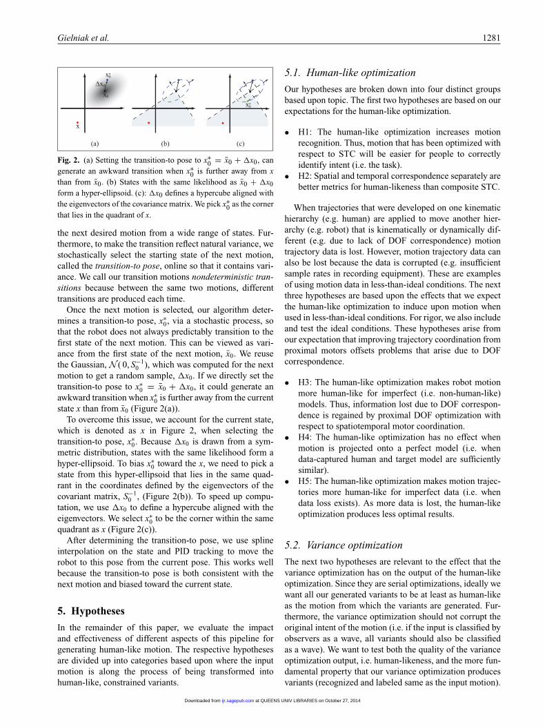
Fig. 2. (a) Setting the transition-to pose to x∗0 = x0 + �x0, can
generate an awkward transition when x∗0 is further away from x
than from x0. (b) States with the same likelihood as x0 + �x0form a hyper-ellipsoid. (c): �x0 defines a hypercube aligned withthe eigenvectors of the covariance matrix. We pick x∗
0 as the cornerthat lies in the quadrant of x.
the next desired motion from a wide range of states. Fur-thermore, to make the transition reflect natural variance, westochastically select the starting state of the next motion,called the transition-to pose, online so that it contains vari-ance. We call our transition motions nondeterministic tran-sitions because between the same two motions, differenttransitions are produced each time.
Once the next motion is selected, our algorithm deter-mines a transition-to pose, x∗
0, via a stochastic process, sothat the robot does not always predictably transition to thefirst state of the next motion. This can be viewed as vari-ance from the first state of the next motion, x0. We reusethe Gaussian, N ( 0, S−1
0 ), which was computed for the nextmotion to get a random sample, �x0. If we directly set thetransition-to pose to x∗
0 = x0 + �x0, it could generate anawkward transition when x∗
0 is further away from the currentstate x than from x0 (Figure 2(a)).
To overcome this issue, we account for the current state,which is denoted as x in Figure 2, when selecting thetransition-to pose, x∗
0. Because �x0 is drawn from a sym-metric distribution, states with the same likelihood form ahyper-ellipsoid. To bias x∗
0 toward the x, we need to pick astate from this hyper-ellipsoid that lies in the same quad-rant in the coordinates defined by the eigenvectors of thecovariant matrix, S−1
0 , (Figure 2(b)). To speed up compu-tation, we use �x0 to define a hypercube aligned with theeigenvectors. We select x∗
0 to be the corner within the samequadrant as x (Figure 2(c)).
After determining the transition-to pose, we use splineinterpolation on the state and PID tracking to move therobot to this pose from the current pose. This works wellbecause the transition-to pose is both consistent with thenext motion and biased toward the current state.
5. Hypotheses
In the remainder of this paper, we evaluate the impactand effectiveness of different aspects of this pipeline forgenerating human-like motion. The respective hypothesesare divided up into categories based upon where the inputmotion is along the process of being transformed intohuman-like, constrained variants.
5.1. Human-like optimization
Our hypotheses are broken down into four distinct groupsbased upon topic. The first two hypotheses are based on ourexpectations for the human-like optimization.
• H1: The human-like optimization increases motionrecognition. Thus, motion that has been optimized withrespect to STC will be easier for people to correctlyidentify intent (i.e. the task).
• H2: Spatial and temporal correspondence separately arebetter metrics for human-likeness than composite STC.
When trajectories that were developed on one kinematichierarchy (e.g. human) are applied to move another hier-archy (e.g. robot) that is kinematically or dynamically dif-ferent (e.g. due to lack of DOF correspondence) motiontrajectory data is lost. However, motion trajectory data canalso be lost because the data is corrupted (e.g. insufficientsample rates in recording equipment). These are examplesof using motion data in less-than-ideal conditions. The nextthree hypotheses are based upon the effects that we expectthe human-like optimization to induce upon motion whenused in less-than-ideal conditions. For rigor, we also includeand test the ideal conditions. These hypotheses arise fromour expectation that improving trajectory coordination fromproximal motors offsets problems that arise due to DOFcorrespondence.
• H3: The human-like optimization makes robot motionmore human-like for imperfect (i.e. non-human-like)models. Thus, information lost due to DOF correspon-dence is regained by proximal DOF optimization withrespect to spatiotemporal motor coordination.
• H4: The human-like optimization has no effect whenmotion is projected onto a perfect model (i.e. whendata-captured human and target model are sufficientlysimilar).
• H5: The human-like optimization makes motion trajec-tories more human-like for imperfect data (i.e. whendata loss exists). As more data is lost, the human-likeoptimization produces less optimal results.
5.2. Variance optimization
The next two hypotheses are relevant to the effect that thevariance optimization has on the output of the human-likeoptimization. Since they are serial optimizations, ideally wewant all our generated variants to be at least as human-likeas the motion from which the variants are generated. Fur-thermore, the variance optimization should not corrupt theoriginal intent of the motion (i.e. if the input is classified byobservers as a wave, all variants should also be classifiedas a wave). We want to test both the quality of the varianceoptimization output, i.e. human-likeness, and the more fun-damental property that our variance optimization producesvariants (recognized and labeled same as the input motion).
at QUEENS UNIV LIBRARIES on October 27, 2014ijr.sagepub.comDownloaded from
1282 The International Journal of Robotics Research 32(11)
• H6: The variance optimization preserves human-likeness.
• H7: The variance optimization preserves intent in theoriginal motion.
5.3. Constraints
Our final three hypotheses test the effect of applied con-straints on human-likeness and variance. The effects of con-straints are tested in terms of both number of constraints andproximity of constraints to DOFs.
• H8: As the number of applied constraints increases,motion becomes less coordinated and less human-like.
• H9: As the number of applied constraints increases,variance decreases.
• H10: Closer to location of application of a Carte-sian constraint, the variance optimization produces lessvariance due to a smaller null space.
6. Experiment 1: Mimicking
The purpose of our first experiment is to quantitatively sup-port that increasing STC of distributed actuators synthe-sizes motion that is more human-like. Since human motionexhibits spatial and temporal correspondence, robot motionthat is more coordinated with respect to space and tim-ing should be more human-like. Thus, we hypothesize thatmotor coordination as produced by SC and TC is a metricfor human-like motion.
Testing this hypothesis requires a quantitative wayto measure human-likeness. Distance measures betweenhuman and robot motion variables (e.g. torques, jointangles, joint velocities) in joint space cannot be used with-out retargeting (i.e. a domain change) due to the DOF cor-respondence problem. Thus, we designed an experimentbased on mimicking.
In short, people are asked to mimic robot motions createdby different motion synthesis techniques, and the techniquethat produced motions that humans were able to mimic the“best” (to be defined later) is deemed the technique thatgenerates the most human-like motion. This experimentassumes that a human-like motion should be easier for peo-ple to mimic accurately, and awkward, less natural motionsshould be harder to mimic.
6.1. Experimental design
In this experiment human motion was measured with aVicon motion capture system. We examined differences inpeople’s mimicking performance when they attempted tomimic the following three types of stimulus motion:
• Original Human (OH): 20 motions captured from amale human, displayed on a virtual human model thatprecisely matches the marker data (i.e. no retargetingtakes place).
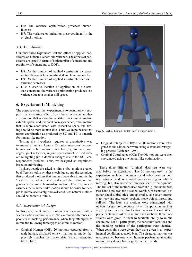
Fig. 3. Virtual human model used in Experiment 1.
• Original Retargeted (OR): The OH motions were retar-geted to the Simon hardware using a standard retarget-ing process (Gleicher, 1998).
• Original Coordinated (OC): The OR motions were thencoordinated using the human-like optimization.
These three different “original” data sets were cre-ated before the experiment. The 20 motions used in theexperiment included common social robot gestures bothunconstrained and constrained, such as waving and object-moving, but also nonsense motions such as “air-guitar”.The full set of the motions used was: shrug, one-hand bow,two-hand bow, scan the distance, worship, presentation, air-guitar, shucks, bird, stick ’em up, cradle, take cover, sneeze,clap, look around, wave, beckon, move object, throw, andcall/yell. The latter six motions were constrained withobjects for gesture directionality or manipulation, such asa box placed in a certain location to wave toward. Whenparticipants were asked to mimic such motions, these con-straints were given to them to facilitate ability to mimicaccurately. For all participants, the constraint locations andthe standing position of the participant were identical.When constraints were given, they were given in all exper-imental conditions to avoid bias. The air-guitar motion wasunconstrained because when humans perform an air-guitarmotion, they do not have a guitar in their hands.
at QUEENS UNIV LIBRARIES on October 27, 2014ijr.sagepub.comDownloaded from
Gielniak et al. 1283
In the experiment, videos of motions were used for dataintegrity and motion repeatability. For example, if the robothardware were used in the motion capture lab, the infraredlight would reflect off the aluminum robot body and cor-rupt data. The original retargeted and original coordinatedmotion trajectories were videotaped on the Simon hardwarefrom multiple angles for the study. Similarly, the originalhuman motion was visualized on a simplified virtual humancharacter (Figure 3) and also recorded from multiple angles.Each video of the recorded motion contained all recordedangles shown serially. There were 60 input (i.e. stimulus)videos total (20 motions for the 3 groups described above).
A total of 41 participants (17 women and 24 men), rang-ing in ages from 20 to 26, were recruited for the study.Each participant saw a set of 12 motions from the possibleset of twenty that were randomly selected for each partici-pant in such a way that each participant received four OH,four OR, and four OC motions each. This provided a set of492 mimicked motions total (i.e. 164 motions from each ofthree groups, with 8–9 mimicked examples for each of 20motions).
6.1.1. Part one: Motion capture data collection Each par-ticipant was equipped with a motion capture suit and toldto observe videos projected onto the wall in the motioncapture lab. They were instructed to observe each motionas long as necessary (without moving) until they thoughtthey could mimic it exactly. The video looped on the screenshowing the motion from different view angles so partici-pants could view each DOF with clarity. Unbeknownst tothem, the number of views before mimicking (NVBM) wasrecorded as a measure for the study.
When the participant indicated they could mimic themotion exactly, the video was turned off and the motioncapture equipment was turned on, and they performed onemotion. Since there is a documented effect of practice oncoordination (Lay et al., 2002), they were not allowed tomove while watching and only their initial performance wascaptured. This process was repeated for the twelve motions.Prior to the 12 motions, each participant was allowed aninitial motion for practice and to get familiar with the exper-imental procedure. Only when a participant was grossly offwith respect to timing or some other anomaly occurred,were suggestions made about their performance before con-tinuing. This happened with two participants, during theirpractice sessions, and those two participants’ non-practicedata is included in the experimental results. No practice datafrom any participant is included in the experimental results.
After mimicking each motion, the participant was askedwhether they recognized the motion, and if so, what namethey would give it (e.g. wave, beckon). Participants did notselect motion names from a list. After mimicking all 12motions, the participant was told the original intent (i.e.name) for all 12 motions in their set. They were then askedto perform each motion unconstrained, as they would nor-mally perform it. This data was recorded with the motion
capture equipment, and in our analysis it is labeled the“participant unconstrained” (PU) set.
While the participants removed the motion capture suit,they were asked which motions were easiest and hardest tomimic; which motions were easiest and hardest to recog-nize; and which motion they thought that they had mim-icked best (TMB). They were asked to give their reasoningbehind all of these choices.
Thus, at the conclusion of part one of Experiment 1, thefollowing data had been collected for each participant:
• Motion capture data from 12 mimicked motions:
– 4 “mimicking human” (MH) motions;– 4 “mimicking retargeted” (MR) motions;– 4 “mimicking coordinated” (MC) motions.
• Number of views before mimicking for each of the 12motions above.
• Recognition (yes/no) for each of the 12 motions.• For all recognizable motions, a name for that motion.• Motion capture data from 12 PU performances of the
12 motions above.• Participant’s selection of:
– easiest motion to mimic, and why;– hardest motion to mimic, and why;– easiest motion to recognize, and why;– hardest motion to recognize, and why;– which motion they thought that they mimicked the
best, and why.
6.1.2. Part two: Video comparison After finishing partone, participants watched pairs of videos for all 12 motionsthat they had just mimicked. Each participant watched theretargeted and coordinated versions (OR and OC) of therobot motion serially, but projected in different spatial loca-tions on the screen to facilitate mental distinction. Theorder of the two versions was randomized. The videos wereshown once each and the participants were asked if theyperceived a difference. Single viewing was chosen becauseit leads to a stronger claim if difference can be noted afteronly one comparison viewing.
Then, the videos were allowed to loop serially and theparticipants were asked to watch the two videos and tellwhich motion in which video they thought looked “bet-ter” and which motion they thought looked more natural.The participants were also asked to give reasons for theirchoices. Unbeknownst to them, the number of views of eachversion before deciding “better” and more natural was alsocollected. The video order for all motions and motion pairswas randomized.
Thus, at the conclusion of part two of Experiment 1, thefollowing data had been collected for each participant:
• Recognized a difference between retargeted and coordi-nated motion after one viewing (yes/no); for each of 12motions mimicked in part one (Section 6.1.1).
at QUEENS UNIV LIBRARIES on October 27, 2014ijr.sagepub.comDownloaded from
1284 The International Journal of Robotics Research 32(11)
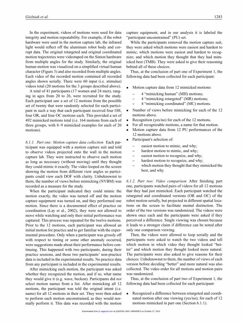
Fig. 4. Percentage of motion recognized correctly, incorrectly, ornot recognized by participants in Experiment 1, for each of thethree categories of original data that they were asked to mimic.Spatiotemporal Coordinated motion is correctly recognized signif-icantly more than simply retargeted motion, and at a rate similarto (but even higher than) the human motion.
• For motions where a difference was acknowledged:
– selection of retargeted or coordinated as “better”;– selection of retargeted or coordinated as more
natural.
• Rationale for “better” and more natural selections.• Number of views before each of these decisions.
6.2. Results
6.2.1. H1: Human-like optimization increases recognitionThe results presented in this section support Hypothesis 1,that our human-like optimization makes robot motion easierto recognize. The data in Figure 4 represents the percentageof participants who named a motion correctly, incorrectly,or who opted not to try to identify the motion (i.e. unrec-ognized). This data is accumulated over all 20 motionsand sorted according to the three categories of stimulusvideo: OH, OR, and OC. Coordinated robot motion wascorrectly recognized 87.2% of the time, and was mistakenlynamed only 9.1% of the time. These are better results thaneither human or retargeted motion. In addition, coordinat-ing motion led human observers to try to identify motionsmore frequently than human or retargeted motion (unrecog-nized = 3.7% for OC, compared with 8.5% for OH and 11%for OR). This data suggests that the human-like optimiza-tion (i.e coordinating motion trajectories) makes the motionmore familiar or common.
On a motion-by-motion basis, the percentage correct washighest for 16 of 20 coordinated motions and lowest for17 of 20 retargeted motions. In 17 of 20 motions percentincorrect was lowest for coordinated motions, and in a dif-ferent set of 17 of 20 possible motions, the percentageincorrect was highest for retargeted motion. These numberssupport the aggregate data presented in Figure 4 suggestingthat naming accuracy, in general, is higher for coordinatedmotion, and lower for retargeted motion. Comparing onlycoordinated and retargeted motion, the percentage correct
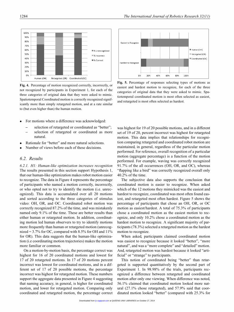
Fig. 5. Percentage of responses selecting types of motions aseasiest and hardest motion to recognize, for each of the threecategories of original data that they were asked to mimic. Spa-tiotemporal coordinated motion is most often selected as easiest,and retargeted is most often selected as hardest.
was highest for 19 of 20 possible motions, and in a differentset of 19 of 20, percent incorrect was highest for retargetedmotion. This data implies that relationships for recogni-tion comparing retargeted and coordinated robot motion aremaintained, in general, regardless of the particular motionperformed. For reference, overall recognition of a particularmotion (aggregate percentage) is a function of the motionperformed. For example, waving was correctly recognized91.7% of the all occurrences (OH, OR, and OC), whereas“flapping like a bird” was correctly recognized overall only40.2% of the time.
The subjective data also supports the conclusion thatcoordinated motion is easier to recognize. When askedwhich of the 12 motions they mimicked was the easiest andhardest to recognize, coordinated was most often found eas-iest, and retargeted most often hardest. Figure 5 shows thepercentage of participants that chose an OH, OR, or OCmotion as easiest/hardest. A total of 75.3% of participantschose a coordinated motion as the easiest motion to rec-ognize, and only 10.2% chose a coordinated motion as thehardest motion to recognize. A significant majority of par-ticipants (78.3%) selected a retargeted motion as the hardestmotion to recognize.
When asked, participants claimed coordinated motionwas easiest to recognize because it looked “better”, “morenatural”, and was a “more complete” and “detailed” motion.And, retargeted motion was hardest because it looked “arti-ficial” or “strange” to participants.
This notion of coordinated being “better” than retar-geted is supported quantitatively by the second part ofExperiment 1. In 98.98% of the trials, participants rec-ognized a difference between retargeted and coordinatedmotion after only one viewing. When difference was noted,56.1% claimed that coordinated motion looked more nat-ural (27.1% chose retargeted), and 57.9% said that coor-dinated motion looked “better” (compared with 25.3% for
at QUEENS UNIV LIBRARIES on October 27, 2014ijr.sagepub.comDownloaded from
Gielniak et al. 1285
retargeted). In the remaining 16.8%, participants (unso-licited) said that “better” or more natural depends on con-text, and therefore they abstained from making a selec-tion. Participants who selected coordinated motion indi-cated they did so because it was a “more detailed” or “morecomplete” motion, closer to their “expectation” of humanmotion.
Statistical significance tests for the results in Figures 4and 5 were not performed due to the nature of the data. Eachnumber is an accumulation expressed as a percentage. Thedata is not forced choice; all participants were trying to cor-rectly recognize the motion; some attempted and failed, andsome did not attempt because they could not recognize themotion.
6.2.2. H2: SC and TC are better than STC The followingresults from Experiment 1 support hypothesis H2, that opti-mizing based on composite STC rather than the individualcomponents of SC and TC produces slightly worse results.
In Equation (3), the individual terms (spatial and tem-poral) on the right-hand side can be evaluated separately,rather than summing to form a composite STC. In ouranalysis, when the components were evaluated individuallyon a motion-by-motion basis, 20 of 20 retargeted motionsexhibited statistical difference (p < 0.05) from the humanmimicked data and 0 of 20 coordinated motions exhibitedcorrespondence that is not statistically different (p < 0.05)than human data distribution. We will discuss these resultsin much more detail in Section 6.2.3. However, with thecomposite STC used as the metric, only 16 of 20 retargetedmotions were statistically different than the original humanperformance (p < 0.05). Since the results were slightly lessstrong when combining the terms and using composite STCas the metric rather than analyzing SC and TC individually,we recommend that the SC and TC individual componentsbe used independently as a metric for human-likeness.
6.2.3. H3: Makes motion human-like Having completedthe discussion on the general hypotheses for our human-likeoptimization, we have not yet completely proven that theoptimization improves human-likeness in the presence ofdifferent models, agents, or data loss. Our robot, discussedin Section 3, represents a model or agent which is differentkinematically and dynamically from a human. Thus, we canuse Experiment 1 data to support our hypotheses regard-ing the effect of the human-like optimization on trajectoriesthat are projected onto kinematic and dynamic hierarchiesof DOFs (e.g. agents, models) that are different. The differ-ence can be the result of DOF correspondence issues, andprojection causes trajectory data loss. We call such trajec-tories: imperfect, which in the instance of Experiment 1,means non-human-like.
The data from Experiment 1 presented in this sectionsupports hypothesis H3, that the human-like optimization(i.e. spatiotemporally coordinating motion) makes robot
motion more human-like. In subsequent sections, hypothe-sis H3 will be refined (via hypotheses H4 and H5, Exper-iments 2 and 3, respectively) to be more general. Thesesubsequent sections will show that for any model or agentthat does not perfectly match the agent (i.e. the originalhuman from which the original trajectory was motion cap-tured or developed) and for large quantities of data loss,the human-like optimization makes any motion trajectorycloser to human-like. This will be true in our case becausethe original trajectories were captured from a human.
Four sets of motion-capture data exist from Experiment1, part one (Section 6.1.1.): MH, MR, MC, and PU motion.Analysis must occur on a motion-by-motion basis. Thus,for each of the 20 motions, there is a distribution of datathat captures how well participants mimicked each motion.For each participant, we calculated the spatial and temporalcorrespondence according to Equation (3), which resolvedeach motion into two numbers, one for each term on theright-hand side of the equation. For each motion, eight ornine participants mimicked OH, OR, and OC. Three timesmore data exists for the unconstrained version becauseregardless which constrained version a participant mim-icked, they were still asked to perform the motion uncon-strained. Thus, for the analysis, we resolved MH, MR, MC,and PU into distributions for SC and TC across all partic-ipants. There are separate distributions for each of the 20motions, yielding 4 × 2 × 20 unique distributions. The goalwas to analyze each of the SC and TC results independentlyon a motion-by-motion basis, in order to draw conclusionsabout MH, MR, MC, and PU. We used analyses of variance(ANOVAs) to test the following hypotheses:
• H3.1: Human motion is not independent of constraint.In other words, all of the human motion capture datasets (MH, MR, MC, and PU) do not have significantlydifferent distributions. The F values, for all 20 motions,ranged from 7.2–10.8 (spatial) and 6.9–7.6 (temporal)which are greater than Fcrit = 2.8. Therefore, we con-cluded at least one of these distributions is differentfrom the others with respect to SC and TC.
• H3.2: Mimicked motion is not independent of con-straint. In other words, all mimicked (i.e. constrained)data, (MH, MR, and MC) do not have significantlydifferent distributions. In these ANOVA tests, valuesfor all 20 motions ranged between 6.1–8.6 (spatial)and 5.3–6.6 (temporal), which are greater than Fcrit =3.4–3.5. Therefore, we concluded that at least one ofthese distributions for mimicked motion is statisticallydifferent.
• H3.3: Coordinated motion is indistinguishable fromhuman motion in terms of SC and TC. MH, MC, andPU sets do not have significantly different distributions.Values for Fobserved of 0.6–1.1 (spatial) and 0.9–1.9(temporal), which are less than Fcrit of 3.2–3.3, mean-ing that with this data there was insufficient evidence toreject this hypothesis for all 20 motions.
at QUEENS UNIV LIBRARIES on October 27, 2014ijr.sagepub.comDownloaded from
1286 The International Journal of Robotics Research 32(11)
Table 1. Student’s t-test results of spatial correspondence fromExperiment 1. Number of motions with p < 0.05 for pair-wise spatial correspondence comparison t-tests for the indicatedstudy variables. Note: The table for temporal correspondence isidentical.
OH OR OC MH MR MC PU
OH X 20 0 0 20 0 0OR X X 20 20 20 20 20OC X X X 0 20 0 0MH X X X X 20 0 0MR X X X X X 20 20MC X X X X X X 0PU X X X X X X X
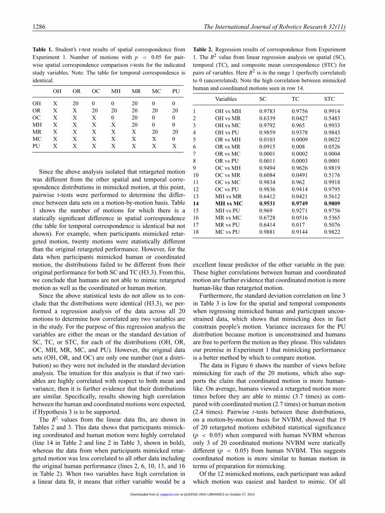
Since the above analysis isolated that retargeted motionwas different from the other spatial and temporal corre-spondence distributions in mimicked motion, at this point,pairwise t-tests were performed to determine the differ-ence between data sets on a motion-by-motion basis. Table1 shows the number of motions for which there is astatically significant difference in spatial correspondence(the table for temporal correspondence is identical but notshown). For example, when participants mimicked retar-geted motion, twenty motions were statistically differentthan the original retargeted performance. However, for thedata when participants mimicked human or coordinatedmotion, the distributions failed to be different from theiroriginal performance for both SC and TC (H3.3). From this,we conclude that humans are not able to mimic retargetedmotion as well as the coordinated or human motion.
Since the above statistical tests do not allow us to con-clude that the distributions were identical (H3.3), we per-formed a regression analysis of the data across all 20motions to determine how correlated any two variables arein the study. For the purpose of this regression analysis thevariables are either the mean or the standard deviation ofSC, TC, or STC, for each of the distributions (OH, OR,OC, MH, MR, MC, and PU). However, the original datasets (OH, OR, and OC) are only one number (not a distri-bution) so they were not included in the standard deviationanalysis. The intuition for this analysis is that if two vari-ables are highly correlated with respect to both mean andvariance, then it is further evidence that their distributionsare similar. Specifically, results showing high correlationbetween the human and coordinated motions were expected,if Hypothesis 3 is to be supported.
The R2 values from the linear data fits, are shown inTables 2 and 3. This data shows that participants mimick-ing coordinated and human motion were highly correlated(line 14 in Table 2 and line 2 in Table 3, shown in bold),whereas the data from when participants mimicked retar-geted motion was less correlated to all other data includingthe original human performance (lines 2, 6, 10, 13, and 16in Table 2). When two variables have high correlation ina linear data fit, it means that either variable would be a
Table 2. Regression results of correspondence from Experiment1. The R2 value from linear regression analysis on spatial (SC),temporal (TC), and composite mean correspondence (STC) forpairs of variables. Here R2 is in the range 1 (perfectly correlated)to 0 (uncorrelated). Note the high correlation between mimickedhuman and coordinated motions seen in row 14.
Variables SC TC STC
1 OH vs MH 0.9783 0.9756 0.99142 OH vs MR 0.6339 0.0427 0.54833 OH vs MC 0.9792 0.965 0.99334 OH vs PU 0.9859 0.9378 0.98435 OR vs MH 0.0103 0.0009 0.00226 OR vs MR 0.0915 0.008 0.05267 OR vs MC 0.0001 0.0002 0.00048 OR vs PU 0.0011 0.0003 0.00019 OC vs MH 0.9494 0.9626 0.981910 OC vs MR 0.6084 0.0491 0.517611 OC vs MC 0.9834 0.962 0.991812 OC vs PU 0.9836 0.9414 0.979513 MH vs MR 0.6412 0.0421 0.561214 MH vs MC 0.9531 0.9749 0.980915 MH vs PU 0.969 0.9271 0.975616 MR vs MC 0.6728 0.0516 0.536517 MR vs PU 0.6414 0.017 0.507618 MC vs PU 0.9881 0.9144 0.9822
excellent linear predictor of the other variable in the pair.These higher correlations between human and coordinatedmotion are further evidence that coordinated motion is morehuman-like than retargeted motion.
Furthermore, the standard deviation correlation on line 3in Table 3 is low for the spatial and temporal componentswhen regressing mimicked human and participant uncon-strained data, which shows that mimicking does in factconstrain people’s motion. Variance increases for the PUdistribution because motion is unconstrained and humansare free to perform the motion as they please. This validatesour premise in Experiment 1 that mimicking performanceis a better method by which to compare motion.
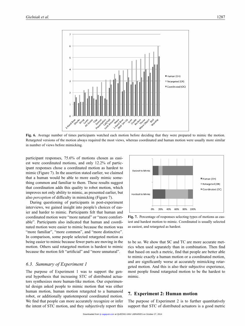
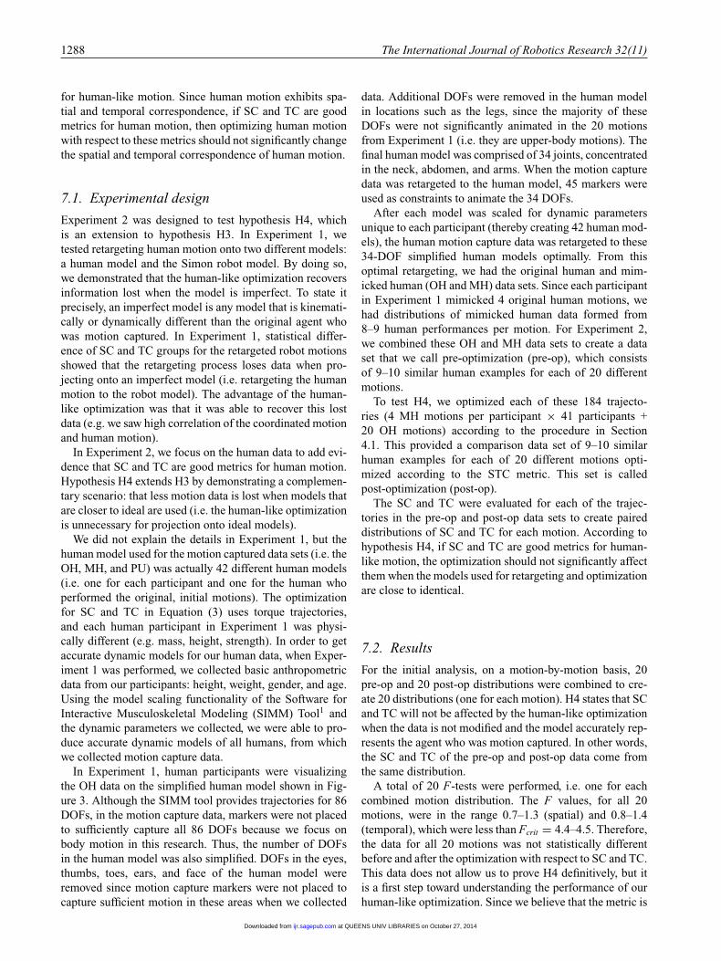
The data in Figure 6 shows the number of views beforemimicking for each of the 20 motions, which also sup-ports the claim that coordinated motion is more human-like. On average, humans viewed a retargeted motion moretimes before they are able to mimic (3.7 times) as com-pared with coordinated motion (2.7 times) or human motion(2.4 times). Pairwise t-tests between these distributions,on a motion-by-motion basis for NVBM, showed that 19of 20 retargeted motions exhibited statistical significance(p < 0.05) when compared with human NVBM whereasonly 3 of 20 coordinated motions NVBM were staticallydifferent (p < 0.05) from human NVBM. This suggestscoordinated motion is more similar to human motion interms of preparation for mimicking.
Of the 12 mimicked motions, each participant was askedwhich motion was easiest and hardest to mimic. Of all
at QUEENS UNIV LIBRARIES on October 27, 2014ijr.sagepub.comDownloaded from
Gielniak et al. 1287
Fig. 6. Average number of times participants watched each motion before deciding that they were prepared to mimic the motion.Retargeted versions of the motion always required the most views, whereas coordinated and human motion were usually more similarin number of views before mimicking.
participant responses, 75.6% of motions chosen as easi-est were coordinated motions, and only 12.2% of partic-ipant responses chose a coordinated motion as hardest tomimic (Figure 7). In the assertion stated earlier, we claimedthat a human would be able to more easily mimic some-thing common and familiar to them. These results suggestthat coordination adds this quality to robot motion, whichimproves not only ability to mimic, as presented earlier, butalso perception of difficulty in mimicking (Figure 7).
During questioning of participants in post-experimentinterviews, we gained insight into people’s choices of eas-ier and harder to mimic. Participants felt that human andcoordinated motion were “more natural” or “more comfort-able”. Participants also indicated that human and coordi-nated motion were easier to mimic because the motion was“more familiar”, “more common”, and “more distinctive”.In comparison, some people selected retargeted motion asbeing easier to mimic because fewer parts are moving in themotion. Others said retargeted motion is hardest to mimicbecause the motion felt “artificial” and “more unnatural”.
6.3. Summary of Experiment 1
The purpose of Experiment 1 was to support the gen-eral hypothesis that increasing STC of distributed actua-tors synthesizes more human-like motion. Our experimen-tal design asked people to mimic motion that was eitherhuman motion, human motion retargeted to a humanoidrobot, or additionally spatiotemporal coordinated motion.We find that people can more accurately recognize or inferthe intent of STC motion, and they subjectively report this
Fig. 7. Percentage of responses selecting types of motions as eas-iest and hardest motion to mimic. Coordinated is usually selectedas easiest, and retargeted as hardest.
to be so. We show that SC and TC are more accurate met-rics when used separately than in combination. Then findthat based on such a metric, find that people are better ableto mimic exactly a human motion or a coordinated motion,and are significantly worse at accurately mimicking retar-geted motion. And this is also their subjective experience,most people found retargeted motion to be the hardest tomimic.
7. Experiment 2: Human motion
The purpose of Experiment 2 is to further quantitativelysupport that STC of distributed actuators is a good metric
at QUEENS UNIV LIBRARIES on October 27, 2014ijr.sagepub.comDownloaded from
1288 The International Journal of Robotics Research 32(11)
for human-like motion. Since human motion exhibits spa-tial and temporal correspondence, if SC and TC are goodmetrics for human motion, then optimizing human motionwith respect to these metrics should not significantly changethe spatial and temporal correspondence of human motion.
7.1. Experimental design
Experiment 2 was designed to test hypothesis H4, whichis an extension to hypothesis H3. In Experiment 1, wetested retargeting human motion onto two different models:a human model and the Simon robot model. By doing so,we demonstrated that the human-like optimization recoversinformation lost when the model is imperfect. To state itprecisely, an imperfect model is any model that is kinemati-cally or dynamically different than the original agent whowas motion captured. In Experiment 1, statistical differ-ence of SC and TC groups for the retargeted robot motionsshowed that the retargeting process loses data when pro-jecting onto an imperfect model (i.e. retargeting the humanmotion to the robot model). The advantage of the human-like optimization was that it was able to recover this lostdata (e.g. we saw high correlation of the coordinated motionand human motion).
In Experiment 2, we focus on the human data to add evi-dence that SC and TC are good metrics for human motion.Hypothesis H4 extends H3 by demonstrating a complemen-tary scenario: that less motion data is lost when models thatare closer to ideal are used (i.e. the human-like optimizationis unnecessary for projection onto ideal models).
We did not explain the details in Experiment 1, but thehuman model used for the motion captured data sets (i.e. theOH, MH, and PU) was actually 42 different human models(i.e. one for each participant and one for the human whoperformed the original, initial motions). The optimizationfor SC and TC in Equation (3) uses torque trajectories,and each human participant in Experiment 1 was physi-cally different (e.g. mass, height, strength). In order to getaccurate dynamic models for our human data, when Exper-iment 1 was performed, we collected basic anthropometricdata from our participants: height, weight, gender, and age.Using the model scaling functionality of the Software forInteractive Musculoskeletal Modeling (SIMM) Tool1 andthe dynamic parameters we collected, we were able to pro-duce accurate dynamic models of all humans, from whichwe collected motion capture data.
In Experiment 1, human participants were visualizingthe OH data on the simplified human model shown in Fig-ure 3. Although the SIMM tool provides trajectories for 86DOFs, in the motion capture data, markers were not placedto sufficiently capture all 86 DOFs because we focus onbody motion in this research. Thus, the number of DOFsin the human model was also simplified. DOFs in the eyes,thumbs, toes, ears, and face of the human model wereremoved since motion capture markers were not placed tocapture sufficient motion in these areas when we collected
data. Additional DOFs were removed in the human modelin locations such as the legs, since the majority of theseDOFs were not significantly animated in the 20 motionsfrom Experiment 1 (i.e. they are upper-body motions). Thefinal human model was comprised of 34 joints, concentratedin the neck, abdomen, and arms. When the motion capturedata was retargeted to the human model, 45 markers wereused as constraints to animate the 34 DOFs.
After each model was scaled for dynamic parametersunique to each participant (thereby creating 42 human mod-els), the human motion capture data was retargeted to these34-DOF simplified human models optimally. From thisoptimal retargeting, we had the original human and mim-icked human (OH and MH) data sets. Since each participantin Experiment 1 mimicked 4 original human motions, wehad distributions of mimicked human data formed from8–9 human performances per motion. For Experiment 2,we combined these OH and MH data sets to create a dataset that we call pre-optimization (pre-op), which consistsof 9–10 similar human examples for each of 20 differentmotions.
To test H4, we optimized each of these 184 trajecto-ries (4 MH motions per participant × 41 participants +20 OH motions) according to the procedure in Section4.1. This provided a comparison data set of 9–10 similarhuman examples for each of 20 different motions opti-mized according to the STC metric. This set is calledpost-optimization (post-op).
The SC and TC were evaluated for each of the trajec-tories in the pre-op and post-op data sets to create paireddistributions of SC and TC for each motion. According tohypothesis H4, if SC and TC are good metrics for human-like motion, the optimization should not significantly affectthem when the models used for retargeting and optimizationare close to identical.
7.2. Results
For the initial analysis, on a motion-by-motion basis, 20pre-op and 20 post-op distributions were combined to cre-ate 20 distributions (one for each motion). H4 states that SCand TC will not be affected by the human-like optimizationwhen the data is not modified and the model accurately rep-resents the agent who was motion captured. In other words,the SC and TC of the pre-op and post-op data come fromthe same distribution.
A total of 20 F-tests were performed, i.e. one for eachcombined motion distribution. The F values, for all 20motions, were in the range 0.7–1.3 (spatial) and 0.8–1.4(temporal), which were less than Fcrit = 4.4–4.5. Therefore,the data for all 20 motions was not statistically differentbefore and after the optimization with respect to SC and TC.This data does not allow us to prove H4 definitively, but itis a first step toward understanding the performance of ourhuman-like optimization. Since we believe that the metric is
at QUEENS UNIV LIBRARIES on October 27, 2014ijr.sagepub.comDownloaded from
Gielniak et al. 1289
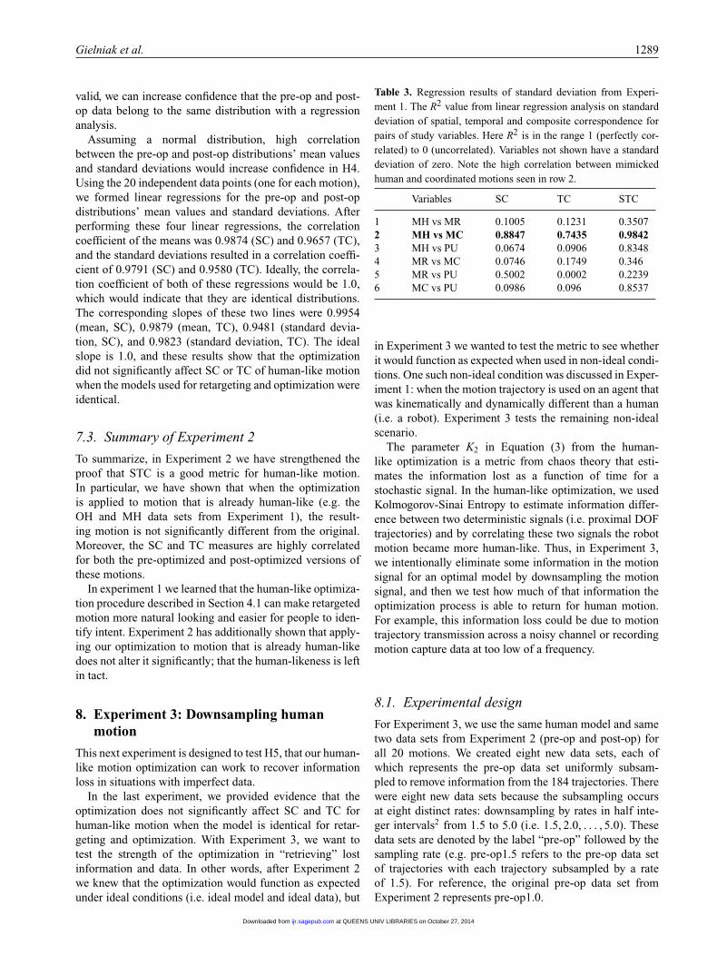
valid, we can increase confidence that the pre-op and post-op data belong to the same distribution with a regressionanalysis.
Assuming a normal distribution, high correlationbetween the pre-op and post-op distributions’ mean valuesand standard deviations would increase confidence in H4.Using the 20 independent data points (one for each motion),we formed linear regressions for the pre-op and post-opdistributions’ mean values and standard deviations. Afterperforming these four linear regressions, the correlationcoefficient of the means was 0.9874 (SC) and 0.9657 (TC),and the standard deviations resulted in a correlation coeffi-cient of 0.9791 (SC) and 0.9580 (TC). Ideally, the correla-tion coefficient of both of these regressions would be 1.0,which would indicate that they are identical distributions.The corresponding slopes of these two lines were 0.9954(mean, SC), 0.9879 (mean, TC), 0.9481 (standard devia-tion, SC), and 0.9823 (standard deviation, TC). The idealslope is 1.0, and these results show that the optimizationdid not significantly affect SC or TC of human-like motionwhen the models used for retargeting and optimization wereidentical.
7.3. Summary of Experiment 2
To summarize, in Experiment 2 we have strengthened theproof that STC is a good metric for human-like motion.In particular, we have shown that when the optimizationis applied to motion that is already human-like (e.g. theOH and MH data sets from Experiment 1), the result-ing motion is not significantly different from the original.Moreover, the SC and TC measures are highly correlatedfor both the pre-optimized and post-optimized versions ofthese motions.
In experiment 1 we learned that the human-like optimiza-tion procedure described in Section 4.1 can make retargetedmotion more natural looking and easier for people to iden-tify intent. Experiment 2 has additionally shown that apply-ing our optimization to motion that is already human-likedoes not alter it significantly; that the human-likeness is leftin tact.
8. Experiment 3: Downsampling humanmotion
This next experiment is designed to test H5, that our human-like motion optimization can work to recover informationloss in situations with imperfect data.
In the last experiment, we provided evidence that theoptimization does not significantly affect SC and TC forhuman-like motion when the model is identical for retar-geting and optimization. With Experiment 3, we want totest the strength of the optimization in “retrieving” lostinformation and data. In other words, after Experiment 2we knew that the optimization would function as expectedunder ideal conditions (i.e. ideal model and ideal data), but
Table 3. Regression results of standard deviation from Experi-ment 1. The R2 value from linear regression analysis on standarddeviation of spatial, temporal and composite correspondence forpairs of study variables. Here R2 is in the range 1 (perfectly cor-related) to 0 (uncorrelated). Variables not shown have a standarddeviation of zero. Note the high correlation between mimickedhuman and coordinated motions seen in row 2.
Variables SC TC STC
1 MH vs MR 0.1005 0.1231 0.35072 MH vs MC 0.8847 0.7435 0.98423 MH vs PU 0.0674 0.0906 0.83484 MR vs MC 0.0746 0.1749 0.3465 MR vs PU 0.5002 0.0002 0.22396 MC vs PU 0.0986 0.096 0.8537
in Experiment 3 we wanted to test the metric to see whetherit would function as expected when used in non-ideal condi-tions. One such non-ideal condition was discussed in Exper-iment 1: when the motion trajectory is used on an agent thatwas kinematically and dynamically different than a human(i.e. a robot). Experiment 3 tests the remaining non-idealscenario.
The parameter K2 in Equation (3) from the human-like optimization is a metric from chaos theory that esti-mates the information lost as a function of time for astochastic signal. In the human-like optimization, we usedKolmogorov-Sinai Entropy to estimate information differ-ence between two deterministic signals (i.e. proximal DOFtrajectories) and by correlating these two signals the robotmotion became more human-like. Thus, in Experiment 3,we intentionally eliminate some information in the motionsignal for an optimal model by downsampling the motionsignal, and then we test how much of that information theoptimization process is able to return for human motion.For example, this information loss could be due to motiontrajectory transmission across a noisy channel or recordingmotion capture data at too low of a frequency.
8.1. Experimental design
For Experiment 3, we use the same human model and sametwo data sets from Experiment 2 (pre-op and post-op) forall 20 motions. We created eight new data sets, each ofwhich represents the pre-op data set uniformly subsam-pled to remove information from the 184 trajectories. Therewere eight new data sets because the subsampling occursat eight distinct rates: downsampling by rates in half inte-ger intervals2 from 1.5 to 5.0 (i.e. 1.5, 2.0, . . . , 5.0). Thesedata sets are denoted by the label “pre-op” followed by thesampling rate (e.g. pre-op1.5 refers to the pre-op data setof trajectories with each trajectory subsampled by a rateof 1.5). For reference, the original pre-op data set fromExperiment 2 represents pre-op1.0.
at QUEENS UNIV LIBRARIES on October 27, 2014ijr.sagepub.comDownloaded from
1290 The International Journal of Robotics Research 32(11)
Then, we optimized each of the 1,472 trajectories(184 × 8) according to the procedure in Section 4.1 to cre-ate an additional eight new data sets for each of 20 motions.This provided paired comparison data sets of 9–10 similarhuman examples of each of 20 different motions for each of8 unique sampling rates optimized according to the SC andTC metrics. These eight data sets are denoted by the label“post-op” followed by the sampling rate (e.g. post-op1.5refers to the pre-op1.5 data set after optimization).
For each trajectory in these 16 new data sets (2,944 tra-jectories), SC and TC were evaluated. According to hypoth-esis H5, if SC and TC are good metrics for human-likemotion, the optimization should compensate for SC and TClost in the downsampling process when the models used forretargeting and optimization are identical. Also, H5 statesthat SC and TC for post-opN trajectories with subsamplingrates closer to 5.0 will be less similar to the pre-op1.0 andpost-op1.0 data sets for each motion.
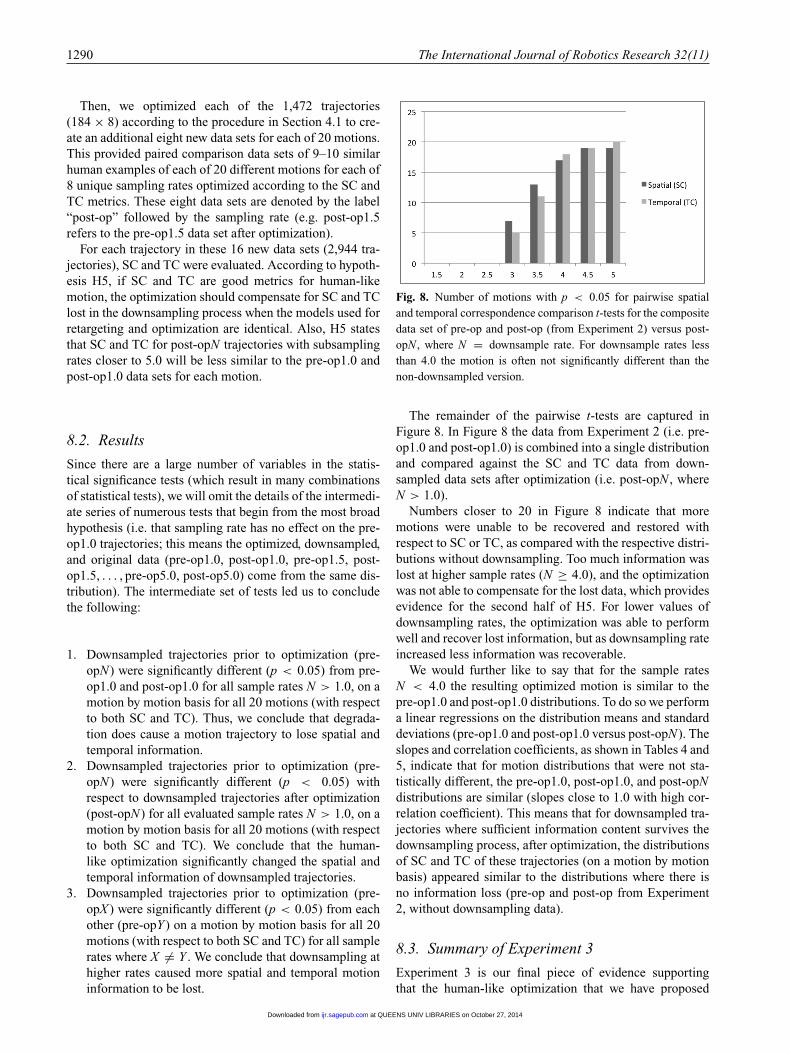
8.2. Results
Since there are a large number of variables in the statis-tical significance tests (which result in many combinationsof statistical tests), we will omit the details of the intermedi-ate series of numerous tests that begin from the most broadhypothesis (i.e. that sampling rate has no effect on the pre-op1.0 trajectories; this means the optimized, downsampled,and original data (pre-op1.0, post-op1.0, pre-op1.5, post-op1.5, . . . , pre-op5.0, post-op5.0) come from the same dis-tribution). The intermediate set of tests led us to concludethe following:
1. Downsampled trajectories prior to optimization (pre-opN) were significantly different (p < 0.05) from pre-op1.0 and post-op1.0 for all sample rates N > 1.0, on amotion by motion basis for all 20 motions (with respectto both SC and TC). Thus, we conclude that degrada-tion does cause a motion trajectory to lose spatial andtemporal information.
2. Downsampled trajectories prior to optimization (pre-opN) were significantly different (p < 0.05) withrespect to downsampled trajectories after optimization(post-opN) for all evaluated sample rates N > 1.0, on amotion by motion basis for all 20 motions (with respectto both SC and TC). We conclude that the human-like optimization significantly changed the spatial andtemporal information of downsampled trajectories.
3. Downsampled trajectories prior to optimization (pre-opX ) were significantly different (p < 0.05) from eachother (pre-opY ) on a motion by motion basis for all 20motions (with respect to both SC and TC) for all samplerates where X �= Y . We conclude that downsampling athigher rates caused more spatial and temporal motioninformation to be lost.
Fig. 8. Number of motions with p < 0.05 for pairwise spatialand temporal correspondence comparison t-tests for the compositedata set of pre-op and post-op (from Experiment 2) versus post-opN , where N = downsample rate. For downsample rates lessthan 4.0 the motion is often not significantly different than thenon-downsampled version.
The remainder of the pairwise t-tests are captured inFigure 8. In Figure 8 the data from Experiment 2 (i.e. pre-op1.0 and post-op1.0) is combined into a single distributionand compared against the SC and TC data from down-sampled data sets after optimization (i.e. post-opN , whereN > 1.0).
Numbers closer to 20 in Figure 8 indicate that moremotions were unable to be recovered and restored withrespect to SC or TC, as compared with the respective distri-butions without downsampling. Too much information waslost at higher sample rates (N ≥ 4.0), and the optimizationwas not able to compensate for the lost data, which providesevidence for the second half of H5. For lower values ofdownsampling rates, the optimization was able to performwell and recover lost information, but as downsampling rateincreased less information was recoverable.
We would further like to say that for the sample ratesN < 4.0 the resulting optimized motion is similar to thepre-op1.0 and post-op1.0 distributions. To do so we performa linear regressions on the distribution means and standarddeviations (pre-op1.0 and post-op1.0 versus post-opN). Theslopes and correlation coefficients, as shown in Tables 4 and5, indicate that for motion distributions that were not sta-tistically different, the pre-op1.0, post-op1.0, and post-opNdistributions are similar (slopes close to 1.0 with high cor-relation coefficient). This means that for downsampled tra-jectories where sufficient information content survives thedownsampling process, after optimization, the distributionsof SC and TC of these trajectories (on a motion by motionbasis) appeared similar to the distributions where there isno information loss (pre-op and post-op from Experiment2, without downsampling data).
8.3. Summary of Experiment 3
Experiment 3 is our final piece of evidence supportingthat the human-like optimization that we have proposed
at QUEENS UNIV LIBRARIES on October 27, 2014ijr.sagepub.comDownloaded from
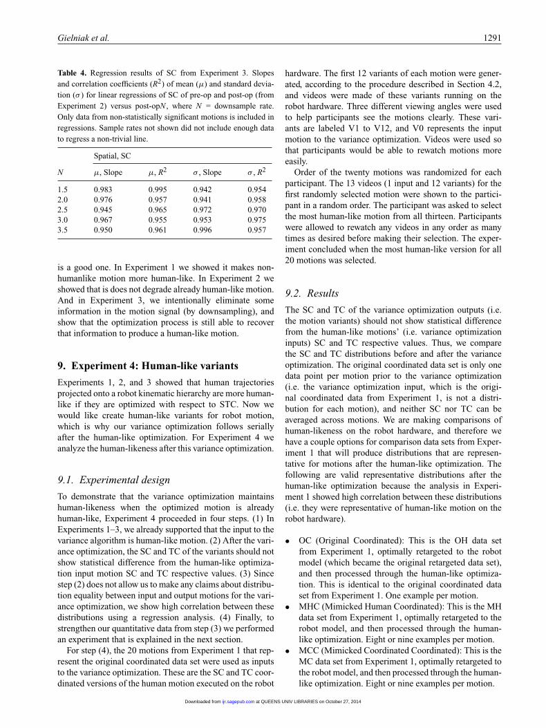
Gielniak et al. 1291
Table 4. Regression results of SC from Experiment 3. Slopesand correlation coefficients (R2) of mean (μ) and standard devia-tion (σ ) for linear regressions of SC of pre-op and post-op (fromExperiment 2) versus post-opN , where N = downsample rate.Only data from non-statistically significant motions is included inregressions. Sample rates not shown did not include enough datato regress a non-trivial line.
Spatial, SC
N μ, Slope μ, R2 σ , Slope σ , R2
1.5 0.983 0.995 0.942 0.9542.0 0.976 0.957 0.941 0.9582.5 0.945 0.965 0.972 0.9703.0 0.967 0.955 0.953 0.9753.5 0.950 0.961 0.996 0.957
is a good one. In Experiment 1 we showed it makes non-humanlike motion more human-like. In Experiment 2 weshowed that is does not degrade already human-like motion.And in Experiment 3, we intentionally eliminate someinformation in the motion signal (by downsampling), andshow that the optimization process is still able to recoverthat information to produce a human-like motion.
9. Experiment 4: Human-like variants
Experiments 1, 2, and 3 showed that human trajectoriesprojected onto a robot kinematic hierarchy are more human-like if they are optimized with respect to STC. Now wewould like create human-like variants for robot motion,which is why our variance optimization follows seriallyafter the human-like optimization. For Experiment 4 weanalyze the human-likeness after this variance optimization.
9.1. Experimental design
To demonstrate that the variance optimization maintainshuman-likeness when the optimized motion is alreadyhuman-like, Experiment 4 proceeded in four steps. (1) InExperiments 1–3, we already supported that the input to thevariance algorithm is human-like motion. (2) After the vari-ance optimization, the SC and TC of the variants should notshow statistical difference from the human-like optimiza-tion input motion SC and TC respective values. (3) Sincestep (2) does not allow us to make any claims about distribu-tion equality between input and output motions for the vari-ance optimization, we show high correlation between thesedistributions using a regression analysis. (4) Finally, tostrengthen our quantitative data from step (3) we performedan experiment that is explained in the next section.
For step (4), the 20 motions from Experiment 1 that rep-resent the original coordinated data set were used as inputsto the variance optimization. These are the SC and TC coor-dinated versions of the human motion executed on the robot
hardware. The first 12 variants of each motion were gener-ated, according to the procedure described in Section 4.2,and videos were made of these variants running on therobot hardware. Three different viewing angles were usedto help participants see the motions clearly. These vari-ants are labeled V1 to V12, and V0 represents the inputmotion to the variance optimization. Videos were used sothat participants would be able to rewatch motions moreeasily.
Order of the twenty motions was randomized for eachparticipant. The 13 videos (1 input and 12 variants) for thefirst randomly selected motion were shown to the partici-pant in a random order. The participant was asked to selectthe most human-like motion from all thirteen. Participantswere allowed to rewatch any videos in any order as manytimes as desired before making their selection. The exper-iment concluded when the most human-like version for all20 motions was selected.
9.2. Results
The SC and TC of the variance optimization outputs (i.e.the motion variants) should not show statistical differencefrom the human-like motions’ (i.e. variance optimizationinputs) SC and TC respective values. Thus, we comparethe SC and TC distributions before and after the varianceoptimization. The original coordinated data set is only onedata point per motion prior to the variance optimization(i.e. the variance optimization input, which is the origi-nal coordinated data from Experiment 1, is not a distri-bution for each motion), and neither SC nor TC can beaveraged across motions. We are making comparisons ofhuman-likeness on the robot hardware, and therefore wehave a couple options for comparison data sets from Exper-iment 1 that will produce distributions that are represen-tative for motions after the human-like optimization. Thefollowing are valid representative distributions after thehuman-like optimization because the analysis in Experi-ment 1 showed high correlation between these distributions(i.e. they were representative of human-like motion on therobot hardware).
• OC (Original Coordinated): This is the OH data setfrom Experiment 1, optimally retargeted to the robotmodel (which became the original retargeted data set),and then processed through the human-like optimiza-tion. This is identical to the original coordinated dataset from Experiment 1. One example per motion.
• MHC (Mimicked Human Coordinated): This is the MHdata set from Experiment 1, optimally retargeted to therobot model, and then processed through the human-like optimization. Eight or nine examples per motion.
• MCC (Mimicked Coordinated Coordinated): This is theMC data set from Experiment 1, optimally retargeted tothe robot model, and then processed through the human-like optimization. Eight or nine examples per motion.
at QUEENS UNIV LIBRARIES on October 27, 2014ijr.sagepub.comDownloaded from
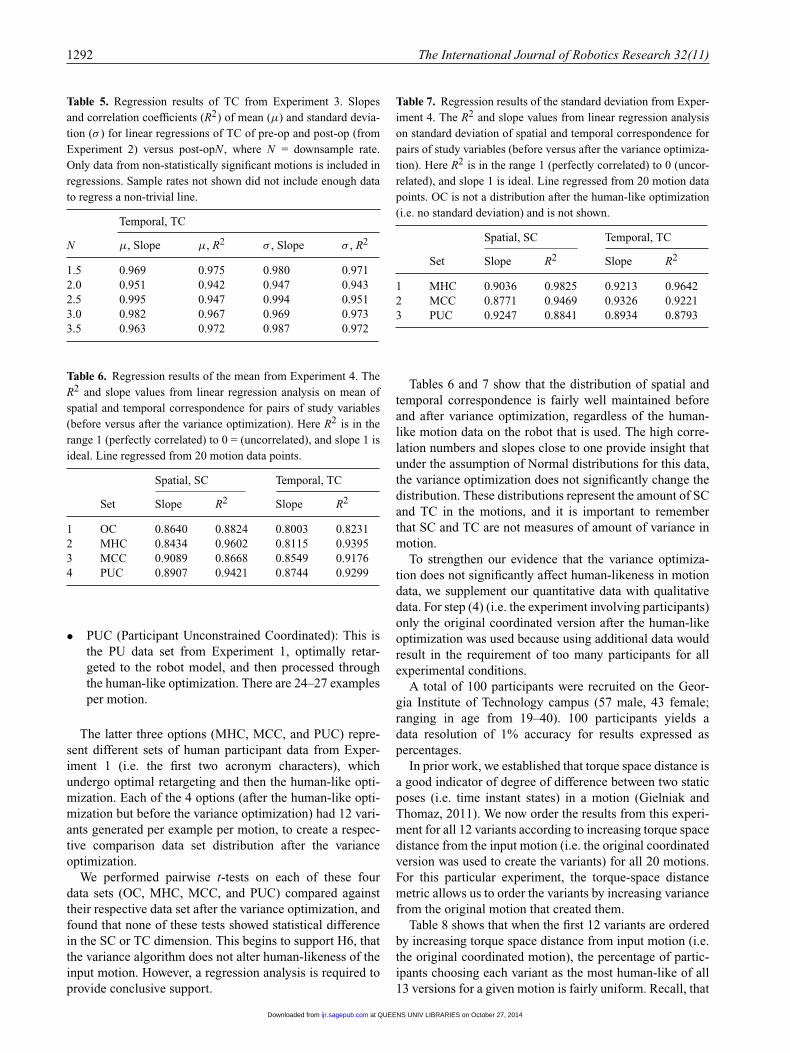
1292 The International Journal of Robotics Research 32(11)
Table 5. Regression results of TC from Experiment 3. Slopesand correlation coefficients (R2) of mean (μ) and standard devia-tion (σ ) for linear regressions of TC of pre-op and post-op (fromExperiment 2) versus post-opN , where N = downsample rate.Only data from non-statistically significant motions is included inregressions. Sample rates not shown did not include enough datato regress a non-trivial line.
Temporal, TC
N μ, Slope μ, R2 σ , Slope σ , R2
1.5 0.969 0.975 0.980 0.9712.0 0.951 0.942 0.947 0.9432.5 0.995 0.947 0.994 0.9513.0 0.982 0.967 0.969 0.9733.5 0.963 0.972 0.987 0.972
Table 6. Regression results of the mean from Experiment 4. TheR2 and slope values from linear regression analysis on mean ofspatial and temporal correspondence for pairs of study variables(before versus after the variance optimization). Here R2 is in therange 1 (perfectly correlated) to 0 = (uncorrelated), and slope 1 isideal. Line regressed from 20 motion data points.
Spatial, SC Temporal, TC
Set Slope R2 Slope R2
1 OC 0.8640 0.8824 0.8003 0.82312 MHC 0.8434 0.9602 0.8115 0.93953 MCC 0.9089 0.8668 0.8549 0.91764 PUC 0.8907 0.9421 0.8744 0.9299
• PUC (Participant Unconstrained Coordinated): This isthe PU data set from Experiment 1, optimally retar-geted to the robot model, and then processed throughthe human-like optimization. There are 24–27 examplesper motion.
The latter three options (MHC, MCC, and PUC) repre-sent different sets of human participant data from Exper-iment 1 (i.e. the first two acronym characters), whichundergo optimal retargeting and then the human-like opti-mization. Each of the 4 options (after the human-like opti-mization but before the variance optimization) had 12 vari-ants generated per example per motion, to create a respec-tive comparison data set distribution after the varianceoptimization.
We performed pairwise t-tests on each of these fourdata sets (OC, MHC, MCC, and PUC) compared againsttheir respective data set after the variance optimization, andfound that none of these tests showed statistical differencein the SC or TC dimension. This begins to support H6, thatthe variance algorithm does not alter human-likeness of theinput motion. However, a regression analysis is required toprovide conclusive support.
Table 7. Regression results of the standard deviation from Exper-iment 4. The R2 and slope values from linear regression analysison standard deviation of spatial and temporal correspondence forpairs of study variables (before versus after the variance optimiza-tion). Here R2 is in the range 1 (perfectly correlated) to 0 (uncor-related), and slope 1 is ideal. Line regressed from 20 motion datapoints. OC is not a distribution after the human-like optimization(i.e. no standard deviation) and is not shown.
Spatial, SC Temporal, TC
Set Slope R2 Slope R2
1 MHC 0.9036 0.9825 0.9213 0.96422 MCC 0.8771 0.9469 0.9326 0.92213 PUC 0.9247 0.8841 0.8934 0.8793
Tables 6 and 7 show that the distribution of spatial andtemporal correspondence is fairly well maintained beforeand after variance optimization, regardless of the human-like motion data on the robot that is used. The high corre-lation numbers and slopes close to one provide insight thatunder the assumption of Normal distributions for this data,the variance optimization does not significantly change thedistribution. These distributions represent the amount of SCand TC in the motions, and it is important to rememberthat SC and TC are not measures of amount of variance inmotion.
To strengthen our evidence that the variance optimiza-tion does not significantly affect human-likeness in motiondata, we supplement our quantitative data with qualitativedata. For step (4) (i.e. the experiment involving participants)only the original coordinated version after the human-likeoptimization was used because using additional data wouldresult in the requirement of too many participants for allexperimental conditions.
A total of 100 participants were recruited on the Geor-gia Institute of Technology campus (57 male, 43 female;ranging in age from 19–40). 100 participants yields adata resolution of 1% accuracy for results expressed aspercentages.
In prior work, we established that torque space distance isa good indicator of degree of difference between two staticposes (i.e. time instant states) in a motion (Gielniak andThomaz, 2011). We now order the results from this experi-ment for all 12 variants according to increasing torque spacedistance from the input motion (i.e. the original coordinatedversion was used to create the variants) for all 20 motions.For this particular experiment, the torque-space distancemetric allows us to order the variants by increasing variancefrom the original motion that created them.
Table 8 shows that when the first 12 variants are orderedby increasing torque space distance from input motion (i.e.the original coordinated motion), the percentage of partic-ipants choosing each variant as the most human-like of all13 versions for a given motion is fairly uniform. Recall, that
at QUEENS UNIV LIBRARIES on October 27, 2014ijr.sagepub.comDownloaded from
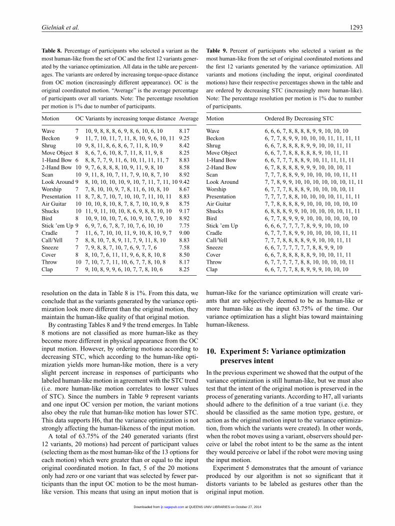
Gielniak et al. 1293
Table 8. Percentage of participants who selected a variant as themost human-like from the set of OC and the first 12 variants gener-ated by the variance optimization. All data in the table are percent-ages. The variants are ordered by increasing torque-space distancefrom OC motion (increasingly different appearance). OC is theoriginal coordinated motion. “Average” is the average percentageof participants over all variants. Note: The percentage resolutionper motion is 1% due to number of participants.
Motion OC Variants by increasing torque distance Average
Wave 7 10, 9, 8, 8, 8, 6, 9, 8, 6, 10, 6, 10 8.17Beckon 9 11, 7, 10, 11, 7, 11, 8, 10, 9, 6, 10, 11 9.25Shrug 10 9, 8, 11, 8, 6, 8, 6, 7, 11, 8, 10, 9 8.42Move Object 8 8, 6, 7, 6, 10, 8, 7, 11, 8, 11, 9, 8 8.251-Hand Bow 6 8, 8, 7, 7, 9, 11, 6, 10, 11, 11, 11, 7 8.832-Hand Bow 10 9, 7, 6, 8, 8, 8, 10, 9, 11, 9, 8, 10 8.58Scan 10 9, 11, 8, 10, 7, 11, 7, 9, 10, 8, 7, 10 8.92Look Around 9 8, 10, 10, 10, 10, 9, 10, 7, 11, 7, 11, 10 9.42Worship 7 7, 8, 10, 10, 9, 7, 8, 11, 6, 10, 8, 10 8.67Presentation 11 8, 7, 8, 7, 10, 7, 10, 10, 7, 11, 10, 11 8.83Air Guitar 10 10, 10, 8, 10, 8, 7, 8, 7, 10, 10, 9, 8 8.75Shucks 10 11, 9, 11, 10, 10, 8, 6, 9, 8, 8, 10, 10 9.17Bird 8 10, 9, 10, 10, 7, 6, 10, 9, 10, 7, 9, 10 8.92Stick ’em Up 9 6, 9, 7, 6, 7, 8, 7, 10, 7, 6, 10, 10 7.75Cradle 7 11, 6, 7, 10, 10, 11, 9, 10, 8, 10, 9, 7 9.00Call/Yell 7 8, 8, 10, 7, 8, 9, 11, 7, 9, 11, 8, 10 8.83Sneeze 7 7, 9, 8, 8, 7, 10, 7, 6, 9, 7, 7, 6 7.58Cover 8 8, 10, 7, 6, 11, 11, 9, 6, 8, 8, 10, 8 8.50Throw 10 7, 10, 7, 7, 11, 10, 6, 7, 7, 8, 10, 8 8.17Clap 7 9, 10, 8, 9, 9, 6, 10, 7, 7, 8, 10, 6 8.25
resolution on the data in Table 8 is 1%. From this data, weconclude that as the variants generated by the variance opti-mization look more different than the original motion, theymaintain the human-like quality of that original motion.
By contrasting Tables 8 and 9 the trend emerges. In Table8 motions are not classified as more human-like as theybecome more different in physical appearance from the OCinput motion. However, by ordering motions according todecreasing STC, which according to the human-like opti-mization yields more human-like motion, there is a veryslight percent increase in responses of participants wholabeled human-like motion in agreement with the STC trend(i.e. more human-like motion correlates to lower valuesof STC). Since the numbers in Table 9 represent variantsand one input OC version per motion, the variant motionsalso obey the rule that human-like motion has lower STC.This data supports H6, that the variance optimization is notstrongly affecting the human-likeness of the input motion.
A total of 63.75% of the 240 generated variants (first12 variants, 20 motions) had percent of participant values(selecting them as the most human-like of the 13 options foreach motion) which were greater than or equal to the inputoriginal coordinated motion. In fact, 5 of the 20 motionsonly had zero or one variant that was selected by fewer par-ticipants than the input OC motion to be the most human-like version. This means that using an input motion that is
Table 9. Percent of participants who selected a variant as themost human-like from the set of original coordinated motions andthe first 12 variants generated by the variance optimization. Allvariants and motions (including the input, original coordinatedmotions) have their respective percentages shown in the table andare ordered by decreasing STC (increasingly more human-like).Note: The percentage resolution per motion is 1% due to numberof participants.
Motion Ordered By Decreasing STC
Wave 6, 6, 6, 7, 8, 8, 8, 8, 9, 9, 10, 10, 10Beckon 6, 7, 7, 8, 9, 9, 10, 10, 10, 11, 11, 11, 11Shrug 6, 6, 7, 8, 8, 8, 8, 9, 9, 10, 10, 11, 11Move Object 6, 6, 7, 7, 8, 8, 8, 8, 8, 9, 10, 11, 111-Hand Bow 6, 6, 7, 7, 7, 8, 8, 9, 10, 11, 11, 11, 112-Hand Bow 6, 7, 8, 8, 8, 8, 9, 9, 9, 10, 10, 10, 11Scan 7, 7, 7, 8, 8, 9, 9, 10, 10, 10, 10, 11, 11Look Around 7, 7, 8, 9, 9, 10, 10, 10, 10, 10, 10, 11, 11Worship 6, 7, 7, 7, 8, 8, 8, 9, 10, 10, 10, 10, 11Presentation 7, 7, 7, 7, 8, 8, 10, 10, 10, 10, 11, 11, 11Air Guitar 7, 7, 8, 8, 8, 8, 9, 10, 10, 10, 10, 10, 10Shucks 6, 8, 8, 8, 9, 9, 10, 10, 10, 10, 10, 11, 11Bird 6, 7, 7, 8, 9, 9, 9, 10, 10, 10, 10, 10, 10Stick ’em Up 6, 6, 6, 7, 7, 7, 7, 8, 9, 9, 10, 10, 10Cradle 6, 7, 7, 7, 8, 9, 9, 10, 10, 10, 10, 11, 11Call/Yell 7, 7, 7, 8, 8, 8, 8, 9, 9, 10, 10, 11, 11Sneeze 6, 6, 7, 7, 7, 7, 7, 7, 8, 8, 9, 9, 10Cover 6, 6, 7, 8, 8, 8, 8, 8, 9, 10, 10, 11, 11Throw 6, 7, 7, 7, 7, 7, 8, 8, 10, 10, 10, 10, 11Clap 6, 6, 7, 7, 7, 8, 8, 9, 9, 9, 10, 10, 10
human-like for the variance optimization will create vari-ants that are subjectively deemed to be as human-like ormore human-like as the input 63.75% of the time. Ourvariance optimization has a slight bias toward maintaininghuman-likeness.
10. Experiment 5: Variance optimizationpreserves intent
In the previous experiment we showed that the output of thevariance optimization is still human-like, but we must alsotest that the intent of the original motion is preserved in theprocess of generating variants. According to H7, all variantsshould adhere to the definition of a true variant (i.e. theyshould be classified as the same motion type, gesture, oraction as the original motion input to the variance optimiza-tion, from which the variants were created). In other words,when the robot moves using a variant, observers should per-ceive or label the robot intent to be the same as the intentthey would perceive or label if the robot were moving usingthe input motion.
Experiment 5 demonstrates that the amount of varianceproduced by our algorithm is not so significant that itdistorts variants to be labeled as gestures other than theoriginal input motion.
at QUEENS UNIV LIBRARIES on October 27, 2014ijr.sagepub.comDownloaded from
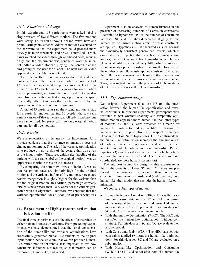
1294 The International Journal of Robotics Research 32(11)
10.1. Experimental design
In this experiment, 153 participants were asked label asingle variant of five different motions. The five motionswere: shrug (i.e. “I don’t know”), beckon, wave, bow, andpoint. Participants watched videos of motions executed onthe hardware so that the experiment could proceed morequickly, be more repeatable, and be well controlled. Partici-pants watched the videos through web-based code, sequen-tially, and the experiment was conducted over the inter-net. After a video stopped playing, the screen blankedand prompted the user for a label. The next motion videoappeared after the label was entered.
The order of the 5 motions was randomized, and eachparticipant saw either the original motion version or 1 of12 variant versions created using our algorithm. For Exper-iment 5, the 12 selected variant versions for each motionwere approximately uniform selections based on torque dis-tance from each other, so that a larger portion of the spaceof visually different motions that can be produced by ouralgorithm could be covered in the analysis.
A total of 33 participants saw the original motion versionfor a particular motion, leaving 10 people who saw eachvariant version of that same motion. All orders and motionswere randomized. No participant saw only original motionversions for all five motions.
10.2. Results
We use recognition as the metric for Experiment 5, toprovide evidence that the variance optimization does notchange motion intent. The task of the variance optimizationis to produce a new version of the gesture that was givenas the input motion. Thus, recognition (i.e. labeling of thevariants with the same label as the original motion), was anappropriate metric to measure the success.
By comparing the bottom two rows in Table 10, we seethat recognition rates are similarly high for the originalmotion and the variants. In four of five motions, percentagecorrect recognition is slightly higher for the variants thanfor the original motion. In addition, percentage correctlylabeled is never more than 0.8% worse for the variants gen-erated with our algorithm. Therefore, we conclude that thevariance optimization does a good job of preserving taskintent.
11. Experiment 6: Highly constrained motionis less human-like
The final three experiments test the effect of constraints oneither human-likeness or variance. From preceding exper-iments, we have demonstrated that the serial concatena-tion of the human-like and variance optimizations havesuccessfully generated human-like variants of the originalinput motion. Since we claim that we can produce human-like, varied motion for robots, it is important to test howconstraints influence our results, so that motion can bepurposeful, human-like, and varied.
Experiment 6 is an analysis of human-likeness in thepresence of increasing numbers of Cartesian constraints.According to hypothesis H8, as the number of constraintsincreases, SC and TC should decrease slightly for thehuman-like optimized motion after Cartesian constraintsare applied. Hypothesis H8 is theorized as such becausethe dynamically consistent generalized inverse, which isessential in the projection that cancels constraint-affectingtorques, does not account for human-likeness. Human-likeness should be affected very little when number ofsimultaneously-applied constraints is small. However, asthe number of simultaneously applied constraints increases,the null space decreases, which means that there is lessredundancy with which to move in a human-like manner.Thus, the resultant motion in the presence of high quantitiesof external constraints will be less human-like.
11.1. Experimental design
We designed Experiment 6 to test H8 and the inter-action between the human-like optimization and exter-nal constraints. In previous experiments, participants wererecruited to test whether spatially and temporally opti-mized motion appeared more human-like than other typesof motions. SC and TC were presented as a metric forhuman-like motion to find a quantitative measure forhumans’ subjective perception with respect to human-likeness in motion. Since hypotheses H1–H5 confirmed thatthe human-like optimization increases the human-likenessof motions, participants no longer need to be recruitedto determine which motions are more human-like. Rather,Equation (3) can be used as a metric to tell which motionsare more human-like (i.e. SC and TC closer to zero, morecoordinated, are more human-like motion).
The intuition behind the design of this experiment isthat if the benefits of lower SC and TC values are pre-served in the presence of constraints, then motion withconstraints remains more coordinated (and therefore, morehuman-like) than motion that excludes the human-like opti-mization.
We compare four types of motion.
• Human Reference Condition (HRC): This is the base-line comparison data set for SC and TC; comprisedof the original human motion and mimicked humanmotion data sets from Experiment 1. For this data set,SC and TC are evaluated on human models.
• With Human-like Optimization (WHO): The HRC dataset after the human-like optimization (without con-straints). For this data set, SC and TC are evaluated ona robot model.
• With Constraints Only (WCO): The HRC data set withconstraints applied (without the human-like optimiza-tion). For this data set, SC and TC are evaluated on arobot model.
• With Human-like Optimization and Constraints(WHC): The HRC data set after both the human-like
at QUEENS UNIV LIBRARIES on October 27, 2014ijr.sagepub.comDownloaded from
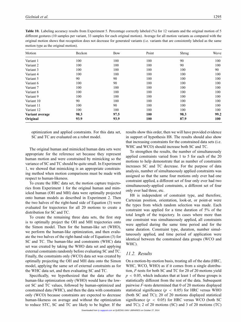
Gielniak et al. 1295
Table 10. Labeling accuracy results from Experiment 5. Percentage correctly labeled (%) for 12 variants and the original motion of 5different gestures (10 samples per variant, 33 samples for each original motion). Average for all motion variants as compared with theoriginal motion shows that recognition does not decrease for generated variants (i.e. variants that are consistently labeled as the samemotion type as the original motion).
Motion Beckon Bow Point Shrug Wave
Variant 1 100 100 100 90 100Variant 2 100 100 100 90 100Variant 3 100 100 100 100 90Variant 4 100 100 100 100 100Variant 5 90 90 100 100 100Variant 6 100 90 100 100 100Variant 7 100 100 100 100 100Variant 8 100 100 100 100 100Variant 9 100 100 100 100 100Variant 10 90 100 100 100 100Variant 11 100 90 100 100 100Variant 12 100 100 100 100 100Variant average 98.3 97.5 100 98.3 99.2Original 93.9 93.9 100 87.9 100
optimization and applied constraints. For this data set,SC and TC are evaluated on a robot model.
The original human and mimicked human data sets wereappropriate for the reference set because they representhuman motion and were constrained by mimicking so thevariance of SC and TC should be quite small. In Experiment1, we showed that mimicking is an appropriate constrain-ing method when motion comparisons must be made withrespect to human-likeness.
To create the HRC data set, the motion capture trajecto-ries from Experiment 1 for the original human and mim-icked human (OH and MH) data were optimally projectedonto human models as described in Experiment 2. Thenthe two halves of the right-hand side of Equation (3) wereevaluated for trajectories for all 20 motions to create adistribution for SC and TC.
To create the remaining three data sets, the first stepis to optimally project the OH and MH trajectories ontothe Simon model. Then for the human-like set (WHO),we perform the human-like optimization, and then evalu-ate the two halves of the right-hand side of Equation (3) forSC and TC. The human-like and constraints (WHC) dataset was created by taking the WHO data set and applyingexternal constraints randomly before evaluating SC and TC.Finally, the constraints only (WCO) data set was created byoptimally projecting the OH and MH data onto the Simonmodel, applying the same set of external constraints as forthe WHC data set, and then evaluating SC and TC.
Specifically, we hypothesized that the data after thehuman-like optimization only (WHO) would have the low-est SC and TC values, followed by human-optimized andconstrained data (WHC), and then the data with constraintsonly (WCO) because constraints are expected to decreasehuman-likeness on average and without the optimizationto reduce STC, SC and TC are likely to be higher. If the
results show this order, then we will have provided evidencein support of hypothesis H8. The results should also showthat increasing constraints for the constrained data sets (i.e.WHC and WCO) should increase both SC and TC.
To strengthen the results, the number of simultaneouslyapplied constraints varied from 1 to 5 for each of the 20motions to help demonstrate that as number of constraintsincreases SC and TC decrease. For the purpose of dataanalysis, number of simultaneously applied constraints wasassigned so that the same four motions only ever had oneconstraint applied, a different set of four only ever had twosimultaneously-applied constraints, a different set of fouronly ever had three, etc.
H8 is independent of constraint type, and therefore,Cartesian position, orientation, look-at, or point-at werethe types from which random selection was made. Eachconstraint was applied for a time duration of 5% of thetotal length of the trajectory. In cases where more thanone constraint was simultaneously applied, all constraintswere applied during the same time period and for thesame duration. Constraint type, duration, number simul-taneously applied, and time period of application wereidentical between the constrained data groups (WCO andWHC).
11.2. Results
On a motion-by-motion basis, treating all of the data (HRC,WHC, WCO, WHO) as if it comes from a single distribu-tion, F-tests for both SC and TC for 20 of 20 motions yieldp < 0.05, which indicates that at least 1 of these groups isstatistically different from the rest of the data. Subsequentpairwise F-tests determined that 0 of 20 motions displayedstatistical significance (p < 0.05) for HRC versus WHO(both SC and TC); 20 of 20 motions displayed statisticalsignificance (p < 0.05) for HRC versus WCO (both SCand TC); 2 of 20 motions (SC) and 3 of 20 motions (TC)
at QUEENS UNIV LIBRARIES on October 27, 2014ijr.sagepub.comDownloaded from
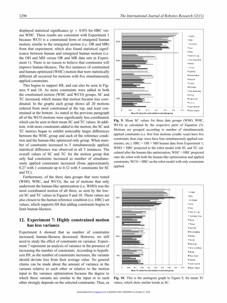
1296 The International Journal of Robotics Research 32(11)
displayed statistical significance (p < 0.05) for HRC ver-sus WHC. These results are consistent with Experiment 1because WCO is a constrained form of retargeted humanmotion, similar to the retargeted motion (i.e. OR and MR)from that experiment, which also found statistical signif-icance between human and retargeted human motion (i.e.the OH and MH versus OR and MR data sets in Experi-ment 1). There is no reason to believe that constraints willimprove human-likeness. The five instances of constrainedand human-optimized (WHC) motion that were statisticallydifferent all occurred for motions with five simultaneouslyapplied constraints.
This begins to support H8, and can also be seen in Fig-ures 9 and 10. As more constraints were added in boththe constrained motion (WHC and WCO) groups, SC andTC increased, which means that motion became less coor-dinated. In the graphs each group shows all 20 motionsordered from most constrained at the top, and least con-strained at the bottom. As stated in the previous paragraphall of the WCO motions were significantly less coordinated,which can be seen in their mean SC and TC values. In addi-tion, with more constraints added to the motion, the SC andTC metrics began to exhibit noticeably larger differencesbetween the WHC group and each of the reference condi-tion and the human-like optimized only group. When num-ber of constraints increased to 5 simultaneously applied,statistical difference was observed in all 5 instances. Theoverall values of SC and TC for the motion group thatonly had constraints increased as number of simultane-ously applied constraints increased (from approximately0.27 with 1 constraint up to 0.32 with 5 constraints for SCand TC).
Furthermore, of the three data groups that were tested(WHO, WHC, and WCO), the set of motions that onlyunderwent the human-like optimization (i.e. WHO) was themost coordinated motion of all three, as seen by the low-est SC and TC values in Figures 9 and 10. These values arealso closest to the human reference condition (i.e. HRC) setvalues, which supports H8 that adding constraints begins tolimit human-likeness.
12. Experiment 7: Highly constrained motionhas less variance
Experiment 6 showed that as number of constraintsincreased, human-likeness decreased. However, we stillneed to study the effect of constraints on variance. Experi-ment 7 represents an analysis of variance in the presence ofincreasing the number of constraints. According to hypoth-esis H9, as the number of constraints increases, the variantsshould deviate less from their average value. No generalclaims can be made about the amount of variance in thevariants relative to each other or relative to the motioninput to the variance optimization because the degree towhich these variants are similar to the input or to eachother strongly depends on the selected constraints. Thus, as
Fig. 9. Mean SC values for three data groups (WHO, WHC,WCO) as calculated by the respective parts of Equation (3).Motions are grouped according to number of simultaneouslyapplied constraints (i.e. first four motions (cradle–scan) have fiveconstraints, then clap–wave have four simultaneously applied con-straints, etc.). HRC = OH + MH human data from Experiment 1;WHO = HRC projected to the robot model with SC and TC cal-culated after the human-like optimization; WHC = HRC projectedonto the robot with both the human-like optimization and appliedconstraints; WCO = HRC on the robot model with only constraintsapplied.
Fig. 10. This is the analogous graph to Figure 9, for mean TCvalues, which show similar trends as SC.
at QUEENS UNIV LIBRARIES on October 27, 2014ijr.sagepub.comDownloaded from
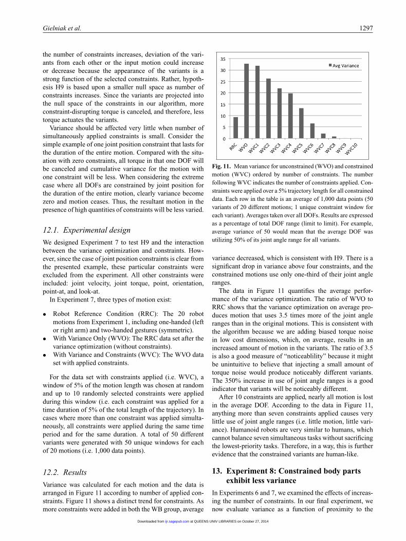
Gielniak et al. 1297
the number of constraints increases, deviation of the vari-ants from each other or the input motion could increaseor decrease because the appearance of the variants is astrong function of the selected constraints. Rather, hypoth-esis H9 is based upon a smaller null space as number ofconstraints increases. Since the variants are projected intothe null space of the constraints in our algorithm, moreconstraint-disrupting torque is canceled, and therefore, lesstorque actuates the variants.
Variance should be affected very little when number ofsimultaneously applied constraints is small. Consider thesimple example of one joint position constraint that lasts forthe duration of the entire motion. Compared with the situ-ation with zero constraints, all torque in that one DOF willbe canceled and cumulative variance for the motion withone constraint will be less. When considering the extremecase where all DOFs are constrained by joint position forthe duration of the entire motion, clearly variance becomezero and motion ceases. Thus, the resultant motion in thepresence of high quantities of constraints will be less varied.
12.1. Experimental design
We designed Experiment 7 to test H9 and the interactionbetween the variance optimization and constraints. How-ever, since the case of joint position constraints is clear fromthe presented example, these particular constraints wereexcluded from the experiment. All other constraints wereincluded: joint velocity, joint torque, point, orientation,point-at, and look-at.
In Experiment 7, three types of motion exist:
• Robot Reference Condition (RRC): The 20 robotmotions from Experiment 1, including one-handed (leftor right arm) and two-handed gestures (symmetric).
• With Variance Only (WVO): The RRC data set after thevariance optimization (without constraints).
• With Variance and Constraints (WVC): The WVO dataset with applied constraints.
For the data set with constraints applied (i.e. WVC), awindow of 5% of the motion length was chosen at randomand up to 10 randomly selected constraints were appliedduring this window (i.e. each constraint was applied for atime duration of 5% of the total length of the trajectory). Incases where more than one constraint was applied simulta-neously, all constraints were applied during the same timeperiod and for the same duration. A total of 50 differentvariants were generated with 50 unique windows for eachof 20 motions (i.e. 1,000 data points).
12.2. Results
Variance was calculated for each motion and the data isarranged in Figure 11 according to number of applied con-straints. Figure 11 shows a distinct trend for constraints. Asmore constraints were added in both the WB group, average
Fig. 11. Mean variance for unconstrained (WVO) and constrainedmotion (WVC) ordered by number of constraints. The numberfollowing WVC indicates the number of constraints applied. Con-straints were applied over a 5% trajectory length for all constraineddata. Each row in the table is an average of 1,000 data points (50variants of 20 different motions; 1 unique constraint window foreach variant). Averages taken over all DOFs. Results are expressedas a percentage of total DOF range (limit to limit). For example,average variance of 50 would mean that the average DOF wasutilizing 50% of its joint angle range for all variants.
variance decreased, which is consistent with H9. There is asignificant drop in variance above four constraints, and theconstrained motions use only one-third of their joint angleranges.
The data in Figure 11 quantifies the average perfor-mance of the variance optimization. The ratio of WVO toRRC shows that the variance optimization on average pro-duces motion that uses 3.5 times more of the joint angleranges than in the original motions. This is consistent withthe algorithm because we are adding biased torque noisein low cost dimensions, which, on average, results in anincreased amount of motion in the variants. The ratio of 3.5is also a good measure of “noticeablility” because it mightbe unintuitive to believe that injecting a small amount oftorque noise would produce noticeably different variants.The 350% increase in use of joint angle ranges is a goodindicator that variants will be noticeably different.
After 10 constraints are applied, nearly all motion is lostin the average DOF. According to the data in Figure 11,anything more than seven constraints applied causes verylittle use of joint angle ranges (i.e. little motion, little vari-ance). Humanoid robots are very similar to humans, whichcannot balance seven simultaneous tasks without sacrificingthe lowest-priority tasks. Therefore, in a way, this is furtherevidence that the constrained variants are human-like.
13. Experiment 8: Constrained body partsexhibit less variance
In Experiments 6 and 7, we examined the effects of increas-ing the number of constraints. In our final experiment, wenow evaluate variance as a function of proximity to the
at QUEENS UNIV LIBRARIES on October 27, 2014ijr.sagepub.comDownloaded from
1298 The International Journal of Robotics Research 32(11)
constraint. Although it might be intuitive that constrainedbody parts will move less, we provide Experiment 8 todemonstrate that constraints work as designed. The pro-jection into the null-space to satisfy Cartesian constraintsshould affect the variance induced by the variance opti-mization more as proximity to the constraint increases.To support H10, Experiment 8 was designed to analyzevariance in the presence of multiple constraints. Cartesianconstraints on the robot’s body force the robot architec-ture to satisfy some geometry: point, line, or plane, whichcauses the constrained body parts to move less in Carte-sian space. Observations such as these motivated hypothesisH10. Robot body parts that are connected in a series chainto a constrained body part will also exhibit less variance.These effects result from the null space because the nullspace is smaller closer to kinematically constrained bodyparts. We test the null space to provide quantitative supportfor hypothesis H10.
13.1. Experimental design
One point constraint and one orientation constraint wereapplied to the robot’s left hand for the entire duration of ashrug trajectory to constrain the hand so that a cup of waterdid not spill. Deviation in the left arm was then analyzedwith respect to the original motion
σh2 = 1
K
1
N
K∑i=1
( q − qi)T ( q − qi) (12)
where σh2 is the average square deviation of DOF h with
respect to original, input motion, qi is the joint angle tra-jectory of DOF h from variant i as a vector, q is the jointangle trajectory of DOF h from the original, input motionas a vector, K is the number of variants used in the analysis,and N is the number of time samples in a given referencetrajectory, and average inter-variant variance
AIVV h = 1
( K − 1)2
1
N
K∑i=1
K∑j=1
( qj − qi)T ( qj − qi), i �= j
(13)
for two conditions: with and without constraints. Compara-ble numbers for constrained and unconstrained conditionson a per-DOF basis would support the null hypothesis thatconstraint projection does not adversely affect variance.This analysis was specifically performed on the arm closestto the constraint because part of hypothesis H10 suggeststhat variance decreases closer to the constrained locationon the architecture.
13.2. Results
To measure variance in the presence of constraints, the vari-ance of the left arm DOFs provided more insight into howconstraints affect the motion because the left arm was closer
to the constraint in the task. We first constrained the originalmotion, and then we used the original motion torques as themean to compute the variance (Equation (12)). The resultsare shown in Table 11.
As expected, physical constraints reduce variance over-all, as shown in Table 11. This was especially true closerto the actual constrained DOF, which for the cup constraintoccurred in the wrist for the x and y DOFs. This effect wasalso evident in the calculations that reference the other vari-ants. However, average variance between variants was stilllarge for the left arm DOFs.
By comparing data for constrained and unconstrained,the trend was that constrained deviation was smaller whenfurther from the wrist (i.e. point of constraint application).The constrained numbers approach unconstrained variancefurther from the wrist, which indicates the impact of con-straints upon variance. From our analysis we concludedthat the variance optimization also produces variance inconstrained motion, provided that a null space for the con-straints exists. H10 is supported since the data clearly indi-cates that variance is limited near the point of applicationof a constraint. As more constraints are added, less variancecan be expected.
14. Discussion
We have presented an algorithm for generating human-likemotion on robots in an autonomous way. Our underlyingassumptions in this work are that: (a) the robot has control-lable, independent actuators; (b) at least one input motionexists; and (c) the robot receives the constraints it mustsatisfy through sensors or a higher-level, decision-makingalgorithm.
Thus, given these assumptions, our algorithm is applica-ble to any robot that needs or wants to move in a more life-like manner. In this work, we have taken significant steps toshow human-likeness, but it is likely that the algorithm willwork for any biologically inspired robot that would havemuscles if it were alive, because animal motion has alsobeen shown to exhibit spatiotemporal coordination due totheir musculature (Hayfron-Acquah et al., 2001).
The three components of our process are as follows.
1. Spatiotemporal coordination: We optimize motion withrespect to STC, which emulates the coordinated effectsof human joints that are connected by muscles.
2. Variance: We add variance to avoid repetitive motionby exploiting redundant and underutilized spaces of theinput motion, which creates multiple motions from asingle input. Possessing multiple versions of the samemotion gives the robot the ability to choose a collision-free path when faced with obstacles.
3. Constraints: We maintain the robot’s ability to inter-act with its world by providing it the ability to satisfyconstraints.
at QUEENS UNIV LIBRARIES on October 27, 2014ijr.sagepub.comDownloaded from
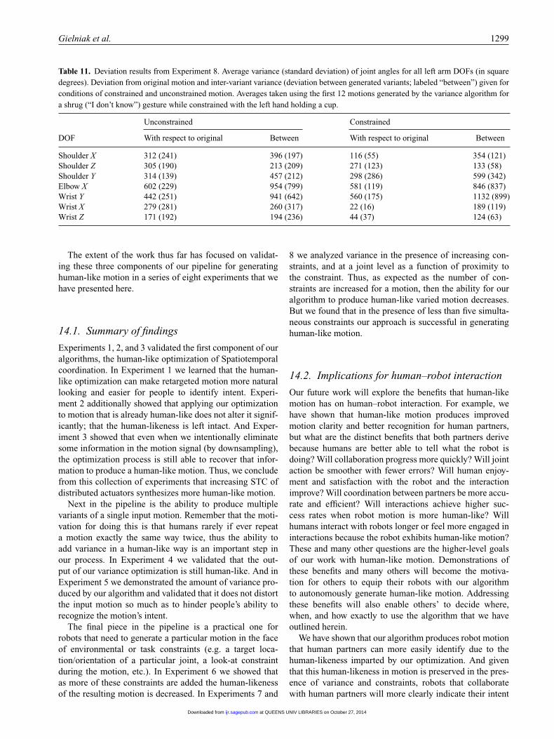
Gielniak et al. 1299
Table 11. Deviation results from Experiment 8. Average variance (standard deviation) of joint angles for all left arm DOFs (in squaredegrees). Deviation from original motion and inter-variant variance (deviation between generated variants; labeled “between”) given forconditions of constrained and unconstrained motion. Averages taken using the first 12 motions generated by the variance algorithm fora shrug (“I don’t know”) gesture while constrained with the left hand holding a cup.
Unconstrained Constrained
DOF With respect to original Between With respect to original Between
Shoulder X 312 (241) 396 (197) 116 (55) 354 (121)Shoulder Z 305 (190) 213 (209) 271 (123) 133 (58)Shoulder Y 314 (139) 457 (212) 298 (286) 599 (342)Elbow X 602 (229) 954 (799) 581 (119) 846 (837)Wrist Y 442 (251) 941 (642) 560 (175) 1132 (899)Wrist X 279 (281) 260 (317) 22 (16) 189 (119)Wrist Z 171 (192) 194 (236) 44 (37) 124 (63)
The extent of the work thus far has focused on validat-ing these three components of our pipeline for generatinghuman-like motion in a series of eight experiments that wehave presented here.
14.1. Summary of findings
Experiments 1, 2, and 3 validated the first component of ouralgorithms, the human-like optimization of Spatiotemporalcoordination. In Experiment 1 we learned that the human-like optimization can make retargeted motion more naturallooking and easier for people to identify intent. Experi-ment 2 additionally showed that applying our optimizationto motion that is already human-like does not alter it signif-icantly; that the human-likeness is left intact. And Exper-iment 3 showed that even when we intentionally eliminatesome information in the motion signal (by downsampling),the optimization process is still able to recover that infor-mation to produce a human-like motion. Thus, we concludefrom this collection of experiments that increasing STC ofdistributed actuators synthesizes more human-like motion.
Next in the pipeline is the ability to produce multiplevariants of a single input motion. Remember that the moti-vation for doing this is that humans rarely if ever repeata motion exactly the same way twice, thus the ability toadd variance in a human-like way is an important step inour process. In Experiment 4 we validated that the out-put of our variance optimization is still human-like. And inExperiment 5 we demonstrated the amount of variance pro-duced by our algorithm and validated that it does not distortthe input motion so much as to hinder people’s ability torecognize the motion’s intent.
The final piece in the pipeline is a practical one forrobots that need to generate a particular motion in the faceof environmental or task constraints (e.g. a target loca-tion/orientation of a particular joint, a look-at constraintduring the motion, etc.). In Experiment 6 we showed thatas more of these constraints are added the human-likenessof the resulting motion is decreased. In Experiments 7 and
8 we analyzed variance in the presence of increasing con-straints, and at a joint level as a function of proximity tothe constraint. Thus, as expected as the number of con-straints are increased for a motion, then the ability for ouralgorithm to produce human-like varied motion decreases.But we found that in the presence of less than five simulta-neous constraints our approach is successful in generatinghuman-like motion.
14.2. Implications for human–robot interaction
Our future work will explore the benefits that human-likemotion has on human–robot interaction. For example, wehave shown that human-like motion produces improvedmotion clarity and better recognition for human partners,but what are the distinct benefits that both partners derivebecause humans are better able to tell what the robot isdoing? Will collaboration progress more quickly? Will jointaction be smoother with fewer errors? Will human enjoy-ment and satisfaction with the robot and the interactionimprove? Will coordination between partners be more accu-rate and efficient? Will interactions achieve higher suc-cess rates when robot motion is more human-like? Willhumans interact with robots longer or feel more engaged ininteractions because the robot exhibits human-like motion?These and many other questions are the higher-level goalsof our work with human-like motion. Demonstrations ofthese benefits and many others will become the motiva-tion for others to equip their robots with our algorithmto autonomously generate human-like motion. Addressingthese benefits will also enable others’ to decide where,when, and how exactly to use the algorithm that we haveoutlined herein.
We have shown that our algorithm produces robot motionthat human partners can more easily identify due to thehuman-likeness imparted by our optimization. And giventhat this human-likeness in motion is preserved in the pres-ence of variance and constraints, robots that collaboratewith human partners will more clearly indicate their intent
at QUEENS UNIV LIBRARIES on October 27, 2014ijr.sagepub.comDownloaded from
1300 The International Journal of Robotics Research 32(11)
to their partners if our algorithm is used to synthesize robotmotion.
This paper revolutionizes trajectory design for robotssince databases of numerous examples of different motionsand complex dynamic equations of motion are no longerrequired to generate variance. Although higher numbersof constraints will restrict variance and human-likenessin robot motion, one exemplar of each motion type (e.g.one wave, one shrug, one reach) is all that is required forthe robot to perform an infinite number of motions simi-lar to the exemplar. That exemplar trajectory can even beobserved to avoid storage issues. Furthermore, we haveshown that imperfect observation of such trajectories is suf-ficient to still create human-like robot motion because ourhuman-like optimization can recover information lost in thetrajectory.
The challenges in using this algorithm are few. The robotrequires a torque trajectory, which means that if the giventrajectory is not in torque-space, inverse dynamics mightneed to be performed on the given trajectory (which wouldrequire a model of the agent from which the exemplar tra-jectory was obtained). The algorithm does not exclude theuse of human motion capture data for the exemplar trajec-tory, but use of such data requires a projection algorithmbetween the human and robot models to provide the inputtrajectory in a proper form.
We also contribute spatial and temporal correspondenceas a metric for human-like motion for robots. The impactof this contribution is that a consistent baseline, which isindependent of kinematics and dynamics, is presented formotion comparison. The independence of this metric meansthat any two agents that have DOFs can have motion com-pared regardless of domain (e.g. cartoon, puppet, robot,human, virtual character). Our metric is the first metric thatcan be used to either evaluate or synthesize human-likemotion. The additional advantages of our metric are thatit is objective, does not require dynamic simulations, and itis not observer- or heavily data-dependent.
Our experiments have also shown that to adequately com-pare human motion data objectively, it must be constrained.We have done so using mimicking, which reduces the vari-ance of the range of motions humans can produce so thatdata is comparable between different humans. Constrainingmotion via mimicking also restricts the variance induceddue to difference in kinematics and dynamics for a humanpopulation, which further facilitates scientific inquiry anddata analysis.
15. Conclusion
We have presented an algorithm that produces human-likevariants of an input motion. This algorithm is made func-tional for real-world tasks by including a projection thatallows the robot to satisfy constraints such as looking at,grabbing, or pointing at objects. Similarly, the algorithmallows robots to synchronize to their partners, provided
that human partners’ actions can be observed. Through aseries of eight experiments, we have shown that human-like robot motion improves recognition accuracy of robotmotions, so that social partners can more easily and accu-rately tell what the robot is doing. This increased clarityin motion can improve collaboration fluidity and minimizedistractions due to awkward robot motion. Variance wasadded to the human-like motion so that human-likenesswould be further improved and robot motion would be lessrepetitive.
Funding
This work was supported by an Office of Naval Research YoungInvestigator Grant (grant number N000140810842) and a NationalScience Foundation CAREER Grant (grant number IIS-1032254).
Notes
1. Trademark of MusculoGraphics Inc. All rights reserved.2. For non-integer subsampling, the rates are represented as a
rational fraction L over M (e.g. 1.5 = 3/2; L = 3; M =2). The data is upsampled by linear interpolation by integer Lfirst, followed by downsampling by integer M .
References
Asfour T, Berns K and Dillmann R (2000) The humanoid robotARMAR: Design and control. In: 1st IEEE-RAS InternationalConference on Humanoid Robots.
Asfour T, Ude A, Berns K and Dillmann R (2001) Controlof ARMAR for the realization of anthropomorphic motionpatterns. In: Second International Conference on HumanoidRobots, pp. 22–24.
Bicho E, Erlhagen W, Louro L and e Silva EC (2011) Neu-rocognitive mechanisms of decision making in joint action:a human-robot interaction study. Human Movement Science30(5): 846–868.
Dasgupta A and Nakamura Y (1999) Making feasible walkingmotion of humanoid robots from human motion capture data.In: Proceedings of the 1999 IEEE International Conference onRobotics and Automation, pp. 1044–1049.
Duffy B (2003) Anthropomorphism and the social robot. Roboticsand Autonomous Systems 42(3–4): 177–190.
Flash T and Hogan N (1985) The coordination of arm move-ments: An experimentally confirmed mathematical model. TheJournal of Neuroscience 5(7): 1688–1703.
Fong T, Nourbakhsh I and Dautenhahn K (2003) A survey ofsocially interactive robots. Robotics and Autonomous Systems42(3–4): 143–166.
Fukuda T, Michelini R, Potkonjak V, Tzafestas S, ValavanisK and Vukobratovic M (2001) How far away is “artificialman”. IEEE Robotics Automation Magazine 8(1): 66–73. DOI:10.1109/100.924367.
Gielniak M and Thomaz AL (2011) Generating anticipation inrobot motion. RO-MAN 31: 449–454
Giese M and Poggio T (2000) Morphable models for the analysisand synthesis of complex motion pattern. International Journalof Computer Vision 38: 59–73.
Gleicher M (1998) Retargeting motion to new characters. In:Proceedings of SIGGRAPH, pp. 33–42.
at QUEENS UNIV LIBRARIES on October 27, 2014ijr.sagepub.comDownloaded from
Gielniak et al. 1301
Harada K, Hauser K, Bretl T and Latombe J (2006) Naturalmotion generation for humanoid robots. In: Proceedings of the2006 IEEE/RSJ International Conference on Intelligent Robotsand Systems, pp. 833–839.
Hayfron-Acquah J, Nixon MS and Carter JN (2001) Recognisinghuman and animal movement by symmetry. In: InternationalConference on Image Processing.
Jenkins O and Mataric M (2004) A Spatiotemporal Extensionto Isomap Nonlinear Dimension Reduction. Technical ReportCRES-04-003, University of Southern California Center forRobotics and Embedded Systems.
Kolmogorov A (1959) Entropy per unit time as a metric invari-ant of automorphisms. Doklady Akademii Nauk SSSR 124:754–755.
Kondo K (1994) Inverse Kinematics of a Human Arm. TechnicalReport CS-TR-94-1508, Stanford University.
Lay B, Sparrow W, Hughes K and O’Dwyer N (2002) Prac-tice effects on coordination and control, metabolic energyexpenditure, and muscle activation. Human Movement Science21(5–6): 807–830. DOI: 10.1016/S0167-9457(02)00166-5.
Lee J, Chai J, Reitsma P, Hodgins J and Pollard N (2002) Inter-active control of avatars animated with human motion data.In: Proceedings of the 29th Annual Conference on ComputerGraphics and Interactive Techniques, pp. 491–500.
Lewis FL and Syrmos VL (1995) Optimal Control. New York:Wiley-Interscience.
Liu C and Popovic Z (2002) Synthesis of complex dynamic char-acter motion from simple animations. In: Proceedings of the29th Annual International Conference on Computer Graphicsand Interactive Techniques, pp. 408–416.
Moeslund T and Granum E (2001) A survey of computer vision-based human motion capture. Computer Vision and ImageUnderstanding 81(3): 231–268.
Oziem D, Campbell N, Dalton C, Gibson D and Thomas B (2004)Combining sampling and autoregression for motion synthe-sis. In: Proceedings of the Computer Graphics InternationalConference. pp. 510–513.
Playter R (2000) Physics-based simulations of running usingmotion capture. In: SIGGRAPH 2000 Course Notes, Course#33.
Popovic Z and Witkin AP (1999) Physically based motiontransformation. In: Proceedings of SIGGRAPH 99. ComputerGraphics Proceedings, Annual Conference Series, pp. 11–20.
Prokopenko M, Gerasimov V and Tanev I (2006) Measuringspatiotemporal coordination in a modular robotic system. In:Rocha LM, Yaeger LS, Bedau MA, Floreano D, GoldstoneRL and Vespignani A (eds), Artificial Life X: Proceedingsof the Tenth International Conference on the Simulation andSynthesis of Living Systems. Cambridge, MA: MIT Press, pp.185–191.
Reitsma P and Pollard N (2003) Perceptual metrics for charac-ter animation: Sensitivity to errors in ballistic motion. ACMTransactions on Graphics 22(3): 537–542.
Ren L, Efros APAA, Hodgins JK and Rehg JM (2005) A data-driven approach to quantifying natural human motion. ACMTransactions on Graphics 24(3): 1090–1097.
Sebanz N, Bekkering H and Knoblich G (2006) Joint action: bod-ies and minds moving together. Trends in Cognitive Science10(2): 70–76.
Sentis L and Khatib O (2006) A whole-body control frameworkfor humanoids operating in human environments. In: IEEEInternational Conference on Robotics and Automation (ICRA),pp. 2641–2648.
Song Y, Goncalves L and Perona P (2003) Unsupervised learningof human motion. IEEE Transactions on Pattern Analysis andMachine Intelligence 25(7): 814–827.
Tomovic R, Bekey G and Karplus W (1987) A strategy for graspsynthesis with multifingered robot hands. In: ProceedingsIEEE International Conference on Robotics and Automation,pp. 83–89.
Wu D (2009) Ad hoc meta-analysis of perceived error in phys-ically simulated characters. In: Game Developers Convention2009. Redmond, WA: Microsoft Game Studios.
Yamane K, Kuffner J and Hodgins J (2004) Synthesizing ani-mations of human manipulation tasks. ACM Transactions onGraphics 23(3): 532–539.
at QUEENS UNIV LIBRARIES on October 27, 2014ijr.sagepub.comDownloaded from
Recommended