Mendel’s Pea
Plant Experiment
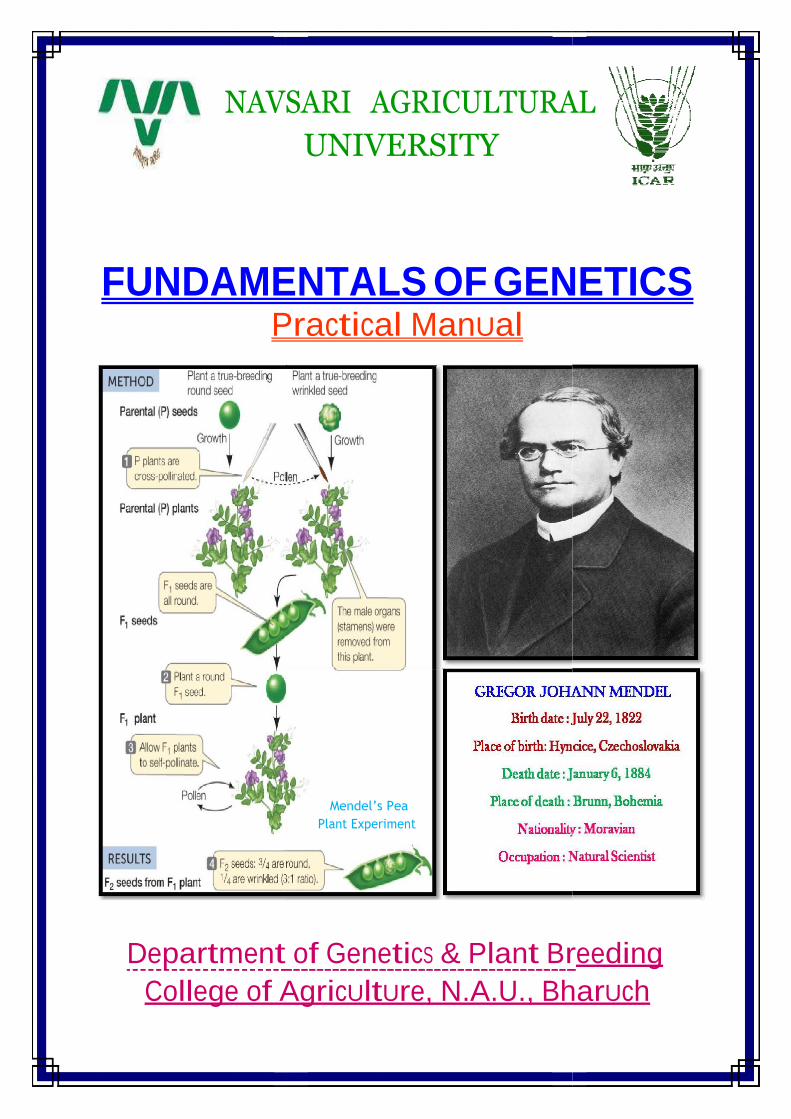
NAVSARI AGRICULTURAL
UNIVERSITY
FUNDAMENTALS OF GENETICS Practical ManUal
Department of GeneticS & Plant Breeding
College of AgricUltUre, N.A.U., BharUch

Reg. No. :-______________________ Roll No. :-_____________________
This is to certify that the practical work has been satisfactory carried out by
Mr. / Ms. ………..………………………………………… in the course No. GPB-3.2
course entitled “Fundamentals of Genetics” (2+1) of 3rd Semester Polytechnic in Agri. In the
laboratory of Department of Genetics and Plant Breeding during the academic year
_________________.
He / She has certified __________ practical exercise out ____________ of in the
subject of “Fundamentals of Genetics”.
External Examiner Course Teacher
Place:
Date:
CERTIFICATE

- - - PRACTICAL MANUAL - - -
FUNDAMENTALS OF GENETICS
--------------------------------------------------------------------------------
INDEX
Ex.
No.
Title Page
No.
Date Sign.
1. Study of Microscopy
2. Study of cell structure and function
3. Preparation of Slide for Mitosis Study
4. Preparation of Slide for Meiosis Study
5. Monohybrid Ratio and its Modification
6. Dihybrid Ratio and its Modification
7. Study of Trihybrid Ratio and back cross methods
8. Chi-Square Analysis
9. Gene Interaction
10. Estimation of Linkage: Two Point Test Cross
11. Estimation of Linkage: Three Point Test Cross

EXERCISE – 1
STUDY OF MICROSCOPY - - - - - - - - - - - - - - - - - - - - - - - - - - - - - - - - - - - - - - - - - - - - - - - - - - - - - - - - - - - - - - - -
A microscope is an instrument used to see objects that are too small for the naked eye. The
science of investigating small objects using such an instrument is called microscopy. In the
laboratory of Genetics, to study cell, cell division processes and ultra structure of chromosomes the
microscope is commonly used. From the primitive observations of protozoan by Antony Van
Leeuwenhoek (1632-1723) to present sophisticated research with fluorescence and interference
optics, the microscope has remained the basic instrument for probing the structural basis of life. The
naked eye is able to distinguish between two points 0.1 mm apart and it is termed as the resolution
power of the eye.
Types of microscopes:
Simple microscopes: The microscopes invented by Leeuwenhoek are considered as simple
microscopes in which a single lens is used as a magnifying glass. A single converging lens in a
simple microscope produces an enlarged real image.
Compound microscopes: The microscopes with a two-lens system and much greater magnification
than simple microscopes are called compound microscopes. A compound microscope has two
lenses (a) the objective lens: It produces an enlarged real image and (b) an eyepiece : It produces a
magnified virtual image of the first enlargement or real image. This is accomplished by the use of
magnifying glasses within the microscope.
Optical microscopes: The microscopes with an optical system in which combination of lenses are
used to enlarge the image of a small object are called optical microscopes. It is a valuable
instrument for studying micro objects, which are too small to be studied with the naked eye. The
resolution power of a good light microscope is 0.2 microns.
When a source of light is present, one can see the object put under the microscope. The light
passing through the slide is partially or completely stopped by objects on the slide and these
objects appear as points of less light or gray images.
If the object is too small to stop waves of light, it cannot be seen with the light microscope.
The observations of biological structures are also difficult to observe under microscope
because cells are in general very small and are transparent to visible light.
Electron microscope: An electron microscope (EM) is a type of microscope that uses
an electron beam to illuminate a specimen and produce a magnified image. An EM has
greater resolving power than a light microscope and can reveal the structure of smaller objects

because electrons have wavelengths about 100,000 times shorter than visible light photons.
They can achieve better than 50 pm resolution and magnifications up to about 10,000,000 X,
whereas ordinary, non-confocal light microscopes are limited by diffraction to about 200
nm resolution and useful magnifications below 2000X. Electron microscopes are used to investigate
the ultra-structure of a wide range of biological and inorganic specimens including microorganisms,
cells, biopsy samples, metals and crystals. Modern electron microscopes produce electron
micrographs using specialized digital cameras or frame grabbers to capture the image.
Fig. 1.1 The Compound Microscope Showing its parts

Parts of the compound microscope and their use:
A microscope has two types of parts,
(a) Optical parts: It includes eye piece, objective lens, condenser, reflecting mirror and iris
diaphragm.
(b) Mechanical parts: It includes all parts of microscope other than the optical parts.
1. Eyepiece or ocular lens: It is the lens present at the top of microscope and is used to see the
objects under study. Eyepiece lens having a magnification of 10X or 15X.
2. Body Tube: It connects the eyepiece to the objective lenses.
3. Revolving nosepiece: It is also known as the turret. Revolving nosepiece has holders for the
different objective lenses, which help to rotate lenses as per the need.
4. Low power objective lens: It is used for observing a relatively large section of the slide. It
magnifies 10X.
5. High power objective lens: It enables us to see a smaller section of the slide in detail. It
magnifies 45X (high-dry).
6. Oil immersion objective lens: This magnifies 100X and is used for observing structures
and organisms at the sub-cellular level. Oil is placed between the slide and the lens to
prevent additional light refraction as it passes from one medium (glass) into another (oil).
The objective produces an enlarged and inverted projection of the object on the other side of
the lens. This first image (a real image) serves as the object for the ocular. The ocular
produces a final image (a virtual image) that is greatly enlarged and still inverted.
7. Iris Diaphragm: Diaphragm helps in controlling the amount of light that is passing through
the opening of the stage. It is helpful in the adjustment of the control of light that enters.
8. Coarse adjustment knob: This is used to bring the objective lens closer to the stage. Turn
this knob and observe the movement of the microscope.
9. Fine adjustment knob: This is also used to bring the objective lens closer to the stage but
relatively on a smaller scale. On turning this knob you cannot see any movement on the
microscope; however, its movement is apparent when one is looking through the
microscope.
10. Arm: It supports the tube of the microscope and connects to the base of the microscope.
11. Stage: The platform that is flat used for placing the slides under observation.
12. Stage clip: Stage clips hold the slides in proper place.
13. Condensor: It focuses the light on the specimen under observation. When very high powers
400X are used, condenser lenses are very important. Presence of condenser lens gives a
sharper image as compared to the microscope with no condenser lens.
14. Base: It provides basal support to the microscope.

Important tips for microscope techniques:
All modern microscopes are parfocal and parcentral.
The term parfocal indicates that the focus does not change appreciably when the objective is
changed; only slight touching up of the focus with the fine adjustment knob is required.
The term parcentral indicates that the centre of the field does not change when the objective
is changed.
When moving the microscope from one place to another, hold it by the arm and carry it
upright.
Always start focusing with the low power first.
Always use the fine adjustment when you are using the high power lens.
While working with the microscope, alternately use both your eyes but keep your both the
Eyes open. This will reduce the stress on your eyes,
To obtain a good image, a cover slip must be used (0.17-0.18 mm thickness) with the high-dry
objective.
Oil-immersion objectives must be used with immersion oil between the front lens and the
cover slip.
Always remember that the oil-immersion objective has a very short working distance and can
easily impact on the slide. When the objective is switched back to high-dry objective, it is
necessary to wipe the immersion oil from the cover slip.
The oil immersion lens should be wiped with a clean lens paper. Dust and body oils on the
lenses dramatically impair quality.
The eye piece (ocular) can be cleaned with lens paper moistened with distilled water.
When the microscope is not in use, it should be covered in wooden box.
What is Refractive Index?
➢ Refraction is the change of direction of a ray of light in passing obliquely from one medium
into another medium in which the speed of transmission differs,
➢ The refractive index of water is the ratio of the speed of light in air to that in water.
➢ R.I. = (Sine of angle of incidence) / (Sine of angle of refraction).
QUESTION BANK
Q-l : Enlist the parts of compound microscope along with its functions.
//*/*/*/*/*//

EXERCISE – 2
Study of cell structure and functions
Cell structure and organelles Cell – It is the structural and functional unit of all living organism
Plant cell : A structural and physiological unit of plant, which have protoplasm.
Cell wall : It is the outermost part of the cell and always non living, tough produced and maintained by
living protoplasm
Cell wall always found in plants cell and absent in animal cell
Functions
1. To protect inner parts of the cell
2. To give a definite shape to the cell
3. To provide mechanical support
Difference between plant cells and animal cells
No Plant cell Animal cell 1. Cell wall present Cell wall absent
2. Chloroplast present Chloroplast absent
3. Plastids occur in cytoplasm Plastids are absent
4. Centrioles are present in cells of lower
plants
Centrioles are present
5. Larger size of vacuoles and are filled with
cell sap
Vacuoles if present are small in size
Labeled diagram of Plant Cell

Label diagram of Animal cell
Cytoplasm
Variety of structure remain suspended such as living and non living
Non living : Non membrane bounded – lipid, starch granules
Living : membrane bounded
Golgi complex : Golgi body first described by Camilo Golgi in 1822 in nerve cell of cat and owl
It is a structure like stalk of filaments arranged one above the other
Composed –Lamellae, tubules, vesicles and vacuoles
Functions :
1. Packaging food materials such as proteins, lipids and phospholipids for transport to other cells
2. It secrete many granules and lysosomes
Lysosomes : The term lysosome was first used by Dave in 1955
In plant cell they are bounded storage granules and containing hydrolylic digestive enzymes
Functions :
1. It is responsible for digestion of intracellular substances and foreign particles.
2. When cell dies lysosomes releases its enzymes, which digest the dead cell resulting in cleaning of
debris.
Ribosomes : Ribosomes are the small cellular particles composed of RNA + Protein
Ribosomes are the site of protein synthesis
They contain nearly 40-60 per cent RNA and other several kinds of protein
In young actively dividing cell they are usually free in the cytoplasm but in the mature cells, they
are attached with ER.
The size or weight of the ribosomes molecules is expressed in S units (sedimentation rate or
coefficient)

Mainly three kinds –
(1) Mitochondrion – 70 S (2) Chloroplastic – 70 S (3) Cytoplasmic – 80 S
Functions :
1. To carry out protein synthesis with the help of m-RNA
Mitochondria : Mitochondria are the rod like cytoplasmic organelle, which is the main site of cellular respiration
They are the source of energy and known as the power house of the cell
Their average number is vary from 200 to 800 per cell
Functions :
1. It involved in respiration, oxidation and metabolism of energy (Power house of the cell)
2. They contain circular DNA and ribosomes, so they are capable of synthesis of certain proteins
3. They contain DNA, so also contribute to heredity by the way of cytoplasmic inheritance
Nucleus and its structure: First discovered by Robert Brown in 1833
Nucleus contains chromosomes and genes, so it known as controlling center of cell
Generally single nucleus per cell
Multi nucleus per cell – protozoa and some fungi (repeated division of nucleus without
cytoplasmic division)
They are spherical or oval shaped
Large in size in active cell than in resting cells
Store house of all genetic information
It consist four parts
1. Nuclear membrane
2. Nucleoplasm
3. Nuclear reticulum
4. Nucleous
Nuclear membrane : 1. Nucleus is enclosed by two membranes of lipo proteins, which separate nucleus and cytoplasm
2. They are not continuous but having several nuclear pores in between
3. Having space between two membrane, which is known as peri nuclear space
4. Outer membrane is attached with ER on which ribosomes are attached
Functions :
It protect the chromosomes from cytoplasmic effects
It permits transport of electrons and exchange of materials between nucleus and cytoplasm
It give rise to some cell organelles
Nucleolus A spherical body found in the nucleus is called nucleolus
It is found in the higher organisms and is attached with specific region of a particular chromosome.
It disappears during prophase of mitosis and meiosis and reappears during telophase.
Chemically it is composed of ribosomal proteins and RNA
Functions :
1. Formation of ribosome and synthesis of proteins
2. It provide energy for all nuclear activities

EXERCISE – 3
PREPARATION OF SLIDE FOR MITOSIS STUDY - - - - - - - - - - - - - - - - - - - - - - - - - - - - - - - - - - - - - - - - - - - - - - - - - - - - - - - - - - - - - - - - - - - -
Cell division
Cell is the basic unit of structure and function of all living systems. The process of
formation of new cells from pre-existing cells is referred as cell division. In cell division process,
the cell going under the division process is referred as mother cell and the new cells which are
formed due to the process of cell division is termed as daughter cells. There are mainly two types of
cell division viz., mitosis and meiosis.
The process of cell division is divided into two parts : (1) Karyokinesis and (2) Cytokinesis
1. Karyokinesis: It is the process of nucleus division.
2. Cytokinesis : It is the process of division of cytoplasm. Cytokinesis follows to karyokinesis.
Preparation of slide for mitosis study
Plant material used for slide preparation : Root tip of onion or somatic cells from shoot tip.
Procedures:
1. Excise the young root tips of onion from plant or germinating onion seeds.
2. Transfer the root tips to vials containing one of the pre-fixatives and keep them at 10 to 14
°C for 2 to 4 hours.
3. Fix the root tips, after washing in water, in carnoy's fluid-I for 24 hours.
4. Root tips are transferred to 70 % ethyl alcohol and keep them at 4 to 10 °C for further use.
5. Put two to three pre-fixed or fixed root tips in a watch glass containing ten drops of 1 %
aceto-orcein and one drop of IN HC1.
6. Heat the watch glass with materials over flame for 10 to 15 seconds in such a way that the
root tip should not come out from stain and then allow them to cool it down.
7. Transfer the root tip to a clean slide and add one to two drops of. 1 % aceto-orcein.
8. The materials are squashed by tapping firmly with a flat end of pencil, metal rod or glass rod
to separate the cells.
9. Put a cover slip and press the slide in folds of blotting paper with the help of thumb to
spread the cells and to remove excess stain.
10. Observed the prepared slide under compound microscope on 10X and then shift it on 45X to
identify the various stages of mitosis.

Cell cycle
Fig. 9.1 Cell cycle with different sub-stages
It is the period in which one cycle of cell division is completed is called cell cycle. It
consists of two phases viz., Interphase and Mitotic phase.
Interphase:
It is the phase of the DNA synthesis in which the chromosomal material is in special stage,
which is known as metabolic stage or interphase. It occupies the time between the end of telophase
of previous mitotic division and the beginning of the next prophase. It occupies the largest period in
a cell cycle. It is often not regarded as a stage of cell division. The interphase is divided into three
sub stages i.e. Gi, S and G2 (Fig-9.1).
1. G1: Synthesis of RNA and protein (Pre DNA replication phase). It occupies 25-50 % of
interphase duration
2. S: Synthesis of DNA (DNA replication phase). It occupies 35-40 % of interphase time

3. G2: Synthesis of mRNA and some fraction of RNA (Post DNA replication phase). It
occupies 15-25 % of interphase duration
During interphase chromosome do not goes any observable cytological changes but
chromosomes are in form of chromatin fibers. While, during mitotic phase (M phase) chromosomes
are duplicated and as a result chromosome number remain constant and definite in each species.
The M phase consists of four stages viz., prophase, metaphase, anaphase and telophase. (Fig 9.2).
Mitosis
The term mitosis was coined by Flemming in 1892. Mitosis refers to the cell division
process in which two identical daughter cells are produced from a mother cell. The chromosome
numbers of newly developed daughter cells are also remaining same as mother cell in mitotic
division. Mitotic division is take place in somatic cells, so it is also referred as a somatic cell
division.
Significance of mitosis:
1. The chief function of the mitosis is growth of organisms and regeneration of damaged
tissues.
2. To keep the chromosome number-constant.
3. It multiplies the cell number and causes vegetative growth and development.
4. Regeneration of damaged tissues and organs.
5. Replacement of old tissues and organs.
6. Production of new tissues and organs like roots, shoots, branches etc.
Stages of mitosis
Mitosis is divided into four different stages viz., (1) Prophase (2) Metaphase (3) Anaphase and (4)
Telophase. (Fig-3.2).
Prophase
Prophase starts immediately after G2 stage of interphase.
o It is the longest mitotic stage.
o Formation of individual chromosome from a chromosomal reticulum.
o Chromosome become shorter, thicker and stains darkly due to condensation and coiling.
o Each chromosome consists of two chromatids and attached at the centromere.
o At the end of prophase nucleolus disappears and nuclear envelop start to breakdown.

Metaphase
o Metaphase phase begins after prophase.
o Metaphase is shorter than prophase but slightly longer than anaphase.
o Nuclear membrane dissolves and formation of spindle fibers takes place.
o Individual chromosomes are arranged at the equatorial plate (metaphase plate).
o The centromere of the each chromosomes serves as its point of orientation
o Each centromere is attached to the spindle fibers.
o Each chromatids of chromosome are clearly visible.
Anaphase
o It is the shortest of all stages in the mitotic cycle.
o The centromere splits longitudinally.
o Two sister chromatids of same chromosome are separated from each other and move
towards opposite poles.
o At end of anaphase, due to contraction of spindle fibers and repulsion forces between newly
formed chromosomes, the daughter chromosomes reach to the respective poles.
o Two groups of chromosomes are visible at each pole.
Telophase
o Uncoiling of chromosome takes place, so that they become long and thin
o The nucleolus and nuclear membrane reappears around each group of daughter
chromosomes
Cytokinesis :
o At the end of telophase, new cell wall is formed at equatorial plate, which divides the
cytoplasm into two equal parts. This process is known as cytokinesis. The division of
cytoplasm into two daughter cells may take place in two ways.
▪ In plants, the division of cytoplasm takes place due to formation of cell plate. The
formation of such plate begins in the center of the cell, which moves towards
periphery in both sides dividing the cytoplasm into two daughter cells.
▪ In animals, the separation of cytoplasm starts by furrowing of plasma lemma in the
equatorial region, which results into division of cytoplasm into two daughter cells.

QUESTION BANK
Q.1: What is mitosis? Write the significance of mitosis.
Q.2: Draw the various stages of mitosis using chromosome number 2n=4.
//*/*/*/*/*//

EXERCISE – 4
PREPARATION OF SLIDE FOR MEIOSIS STUDY - - - - - - - - - - - - - - - - - - - - - - - - - - - - - - - - - - - - - - - - - - - - - - - - - - - - - - - - - - - - - - - - - - - - - - - - - - - - - - - - - -
MEIOSIS
The term meiosis was coined by Moore and Farmer (1905). It is a cell division process in
which, from a single mother cell four haploid daughter cells are produced. The process of meiosis is
divided into two types of division. The first division (meiosis-I) is known as reductional division
and the second division (meiosis-II) is known as equational division.
Important features of the meiosis:
o Meiosis results in the formation of four daughter cells from a single mother cell in each
cycle of cell division.
o Newly developed daughter cells are identical to mother cell in shape and size but it differ in
chromosome number.
o Meiosis occurs in reproductive organs like anthers and ovaries.
o The complete process of meiosis consists of two types of division. The first division results
in the reduction of chromosome number to half (Reductional division) and the second
division is like mitotic division (Equational division).
o Meiosis results in segregation of chromosomes and genes and their independent assortment.
Crossing over and recombination also occurs during meiosis.
Slide preparation for meiosis studies:
Material use for slide preparation: Flower buds
1. First fix the flower buds in Carnoy’s fluid-II solution for 24 hours. Transferred the material
into 70 % alcohol and stored it 10 0C for further use.
2. Open the young flower bud with the help of pointer and collect the anthers.
3. Transfer the anther on a clean slide and add one drop of 2 % aceto-carmine.
4. Crush the anther with the help of pointer and tap it with the flat end of pencil or glass rod.
5. Put a cover slip on the material and heat up the slide gently.
6. Again gently tap the material to separate the cells.
7. Put a blotting paper on it and press it with thumb to remove the excess stains.
8. Finally, observe the prepared slide under the microscope.

Significance/Importance of meiosis :
o Meiosis maintains a definite and constant number of chromosomes from one generation to
the next generation produced by sexual reproduction.
o It facilitates the segregation and independent assortment of chromosomes and genes.
o The recombination of genes takes place during meiosis, which act as the basis of genetic
variation.
STAGES OF MEIOSIS
First meiotic division (Reductional division)
In first meiotic division, the chromosome number of newly developed cells is half in
compared to the mother cell, therefore it is referred as reductional division. It consist four different
phases viz., Prophase-I, Metaphase-I, Anaphase-I and Telophase-I.
1) Prophase –I : This phase consist very long duration and it is sub divided into five stages
viz., Leptotene, Zygotene, Pachytene, Diplotene and Diakinesis.
a) Leptotene :
o Chromosomes look like long, thin thread under light microscope, They are inter woven
like a loose ball of wool.
o Chromosomes are scattered throughout the nucleus in a random manner.
o RNA and protein synthesis also take place.
b) Zygotene :
o Each chromosome divides into two chromatids. Chromatids become clear due to
continuous coiling.
o Chromosomes become shorter and thicker.
o This stage is also characterized by pairing of homologous chromosomes (Synapsis).
o The pairing take place in zipper like fashion and may start at centromere, at chromosome
ends or any other position.
c) Pachytene :
o Chromosomes look like bivalent and each bivalent has now two chromatids. Thus each
chromosome has four chromatids generally known as tetrads.
o In this stage, the chromosome number look likes haploid number (but actually it is
diploid).
o Nucleolus is present and attached to a chromosome.
o Formation of chiasmata and crossing over take place i.e exchange of segments between
non homologous chromatids of homologous chromosomes take place.

d) Diplotene :
o In this stage further thickening and shortening of chromosomes take place.
o Homologous chromosomes start separating from each other. The separation starts from
centromere and proceeds towards terminal end (Chromosome terminalization)
o Homologous chromosomes are held together only at certain point, such points are
referred as chiasma or chiasmata.
o Nucleolus decrease in size.
b) Diakinesis :
o This stage begins after complete terminalization of chiasmata.
o Chromosomes are further condensed.
o Bivalents are distributed throughout the cell.
o Nucleolus and nuclear membrane disappear towards the end of the diakinesis.
Stages of Prophase-I
2) Metaphase - I
o This is the best stage to counting the chromosome number.
o Spindle fibers attached from poles to the centromere.
o Bivalents are arranged at equatorial plate with homologous chromosomes oriented towards
opposite poles.
o Chromatids are clearly visible.
o The centromere of each homologous chromosomes separates from each other.

3) Anaphase - I
o From each bivalent, one homologous chromosome moves toward one pole and another
opposite pole. In another word one homologous chromosomes moves towards one pole and
another to opposite pole.
o Sister chromatids of each chromosome remain attached at the centromere.
o Homologous chromosomes reach the opposite pole at the end of this phase.
4) Telophase - I
o Chromosomes uncoiled and relax and regrouping of chromosome occurs.
o Nucleolus and nuclear membrane reappear.
o Two haploid daughter nuclei are formed.
Cytokinesis :
o At the end of telophase-I, cytoplasm is divided into two halves and each two halves are
staying to gether, this structure is called Dyad.

Second meiotic division (Equational division)
The first meiotic division (meiosis-I) results in reduction of chromosomes number from
diploid to haploid. The second nuclear division (meiosis-II) is required to reduce the number of
chromatids per chromosomes. Meiosis –II differs from mitosis in the following three aspects :
1) The interphase prior to meiosis II is very short. It does not have S phase because each
chromosome already contains two chromatids.
2) The two sister chromatids in each chromosomes are not sister chromatid throughout. In
other words, some chromatids have alternate segments of non sister chromatids due to
recombination.
3) The meiosis-II deals with haploid chromosome number, whereas normal mitosis deals with
diploid chromosome number.
Different stages of meiosis (2n=4)
Rest of the features of meiosis –II is similar to mitosis. It also consist the phases like
prophase-II, metaphase-II, anaphse-II and telophase-II.
1) Prophase - II
o This stage is quite similar to that of mitosis but it differs in several aspects
o There is no relational coiling between sister chromatid, as a result two sister chromatids of
each chromosome are clearly visible.
o The chromosomes are much more condensed and appeared shorter and thicker.
o At the end of prophase, nucleolus and nuclear membrane are disappearing.

2) Metaphase - II
o In this stage, chromosomes become arranged on the equatorial plate.
o Nucleolus and nuclear envelope are absent.
o Spindle apparatus is present and centromere of each chromosome is arranged at the
equatorial plate.
o Two sister chromatids of each chromosome are distinctly separated from each other.
o Chromosomes become more condensed, thicker and shorter.
o The stage is quite short in duration.
3) Anaphase - II
o In this stage, centromere of the each chromosome divides longitudinally.
o Two sister chromatids of each chromosome begins to separate and move away to opposite
poles.
4) Telophase - II
o In this stage, uncoiling of chromosomes take place.
o Reappearance of nucleolus and reformation of nuclear envelop around each group of
chromosomes.
Cytokinesis :
o By the end of telophase- II, the cytoplasm of each of the two cells divides into two parts, so
total four haploid daughter cells are produced after completion of two meiotic divisions.
These four haploid daughter cells are all to gether referred as Tetrad.
o Then this four haploid cells differentiate into gamete and this process is known as
gametogenesis
QUESTION BANK
Q-l: Differentiate the followings:
a) Mitosis and Meiosis
b) Meiosis-I and Meiosis-II
Q-2: What are the significance of mitosis and meiosis.
Q-3: Draw the various stages of meiosis-I & II using the chromosome number 2n=4.
//*/*/*/*/*//

EXERCISE – 5
MONOHYBRID RATIO AND ITS MODIFICATION - - - - - - - - - - - - - - - - - - - - - - - - - - - - - - - - - - - - - - - - - - - - - - - - - - - - - - - - - - - - - - - - - - - -
Monohybrid:
The progeny derived by crossing two genetically dissimilar homozygous parents differing
for one gene pair governing a single character is referred as monohybrid.
Monohybrid ratio:
In case of complete dominance, the phenotypic ratio of monohybrid in F2 generation is 3:1,
it is referred as monohybrid ratio. Mendel has studied the inheritance of only one character at a
time, which helped him to formulate the concept of gene.
Essentials of concept of gene
➢ Development of each character is controlled by a gene,
➢ Each gene exists in two alternate forms called alleles.
➢ Genes are particulate so that two alleles of a gene do not modify each other when they exist
to gather in a same cell.
➢ Each somatic cell having two copies of a gene (identical or distinct alleles), while gamete
have only one copy.
➢ Alleles of a gene separate and pass into different gametes.
➢ Genes are the unit of inheritance passes from one generation to another generation.
Different Terminology:
Character:
Any morphological, anatomical, biochemical features of an individual is known as
character. Each character having two different forms known as contrasting forms or alternative form
of a character.
Example:
1. Plant height: Tall and Dwarf
2. Seed shape : Smooth seed shape and wrinkled seed shape
Dominant character: The character which can express in F1; generation is called as dominant
character.
Recessive character: The character whose effect is masked or suppressed in F1 generation is called
as recessive character.

Mendel has carried out experiments with garden pea (Pisum sativum L.) in a small
monastery garden for seven years and recorded observations on seven different characters. In one of
his experiments, he made a cross between tall and dwarf varieties. The plant height resulting in the
F1 hybrids were all tall type but the F2 generation produced from F1 generation selfing were having
two kinds of height i.e tall and dwarf. Out of every four plant in F2 three were of tall type and one
was dwarf type. The detail experiment is diagrammatically explained in Fig 5.1.
Fig. 5.1: Segregation of plant height character in garden pea
Modifications of monohybrid
There are two kinds of modifications in case of monohybrid
1. Incomplete dominance
2. Codominance
Incomplete dominance (partial dominance):
Mendel has studied seven different characters of garden pea, in which he observed the
complete dominance of one allele over other allele for all studied seven characters. The situation
where complete dominance is observed in those cases clear cut 3 : 1 segregation ratio is observed in
F2 generation for a particular studied character but in certain situation the ratio is deviating, which
indicate the case of incomplete dominance. For example in four '0' clock plant (Mirabilis jalapa)
there are two types of flowers viz., red and white. A cross between red and white flower plants
produced plants with intermediate flower color i.e. pink flower in F1 and it modified the normal
monohybrid F2 ratio (3 red : 1 white) into 1 red : 2 pink : 1 white in F2 generation. (Fig. 5.2).

Incomplete dominance:-
Incomplete dominance refers to a genetic situation in which one allele does not completely
dominate another allele, and therefore results in a new phenotype.
Fig. 5.2: Example of Incomplete Dominance
Codominance:
Allele which lacks the dominant and recessive relationship is called co-dominant alleles or
intermediate alleles.
In case of co-dominance, both alleles express their phenotypes in heterozygote condition.
For example, in case of ABO blood group in human, person having blood group AB are
heterozygote exhibiting the phenotypes of both the IA and I
B alleles.
The difference between codominance and incomplete dominance lies in the way in which
gene acting. In case of codominance, both the alleles are active and expressed in F1, while in case of
incomplete dominance, both the alleles are active but the intensity of expression of dominant allele
is higher in compared to recessive allele and that results into blending effect (mixed effect) of the
character.

QUESTION BANK
Q-l: Define the followings terms:
1) Monohybrid
2) Dominant character
3) Recessive character
4) Inheritance
5) Incomplete dominance
6) Codominance
Q-2: What are the difference between incomplete dominance and codominance.
Q-3: Explain the incomplete dominance using suitable example.
//*/*/*/*/*//

EXERCISE – 6
DIHYBRID RATIO AND ITS MODIFICATION - - - - - - - - - - - - - - - - - - - - - - - - - - - - - - - - - - - - - - - - - - - - - - - - - - - - - - - - - - - - - - - - - - - - - - - - -- - - - - - - -
Dihybrid:
The progeny derived by crossing two genetically dissimilar homozygous parents differing
for two gene pair governing two different characters is referred as dihybrid.
Dihybrid ratio:
In case of complete dominance, the phenotypic ratio of dihybrid in F2 generation is 9: 3: 3:1,
it is referred as dihybrid ratio.
Example:
Mendel had carried out experiments with garden pea (Pisum sativum L.) in a small
monastery garden for seven years and recorded observations on seven different characters. In one of
his experiments, he made a cross between two different varieties, which were differed for two
different characters i.e. seed color and seed shape. One variety had yellow seed color and round
seed shape (YYRR), while the other variety had green seed color and wrinkled seed shape (yyrr).
For seed color, yellow seed color is dominant over green and for seed shape, round seed shape is
dominant over wrinkled. A cross between yellow seed color and round seed shape (YYRR) plant
with green seed color and wrinkled seed shaped (yyrr) plant produced the F1 (YyRr) plants with
yellow color and round seed due to dominant behavior of Y allele over y and R allele over r. The
detail experiment is presented in Fig. 6.1.

In F1 both the gene pair Yy and Rr will segregate simultaneously and according to law of
segregation, Yy gene pair contain half Y gamete and other half y, similarly for Rr gene pair, half the
gamete will contain R and the other half r. A random union of these four alleles of F1 produces four
different types of gametes (YR, Yr, yR and yr) in a equal proportion of 1 : 1 : 1 : 1. This four
different female and male gametes random union leads to development of 16 different zygotic
combinations in F2 generation. Phenotypic ratio in F2:-
9 (Yellow Round): 3 (Yellow Wrinkled) : 3 (Green Round) : 1(Green Wrinkled)
In forming the F2 plants, the alleles at the two loci segregate independently. So, the chance
of getting R allele and Y allele is 1/2 x 1/2, it is also similar for r and y allele. Thus, all four possible
diallelic combinations occur in equal proportions, and each has a probability of 1/4. This is same for
both the parents. Given four possible gamete types in each parent, there are 4 x 4 = 16 possible F2
combinations, and the probability of any particular dihybrid type is 1/4 x 1/4 = 1/16. The
phenotypes and phenotypic ratios of these 16 genotypes can be determined by inspection of the
diagram above called a Punnet Square.
The phenotypic ratio expected for either character is 3 : 1, either 3 "Y" : 1 "y", or 3 "R" : 1
"r". Then, algebra tells us that (3Y + ly) x (3R + lr) = 9YR : 3Yr : 3Ry : 1 ry. We expect a
characteristic 9:3:3:1 phenotypic ratio of Yellow Round : Yellow Wrinkled : Green Round : Green
Wrinkled combination.
To predict the genotypic ratios, recall that for a single gene the genotypic ratio is 1:2:1 -AA:Aa:aa .
Then, algebraically
(1YY + 2Yy + lyy) x (1RR + 2Rr + lrr) = 1 YYRR + 2 YYRr + 1 YYrr + 2YyRR + 4YyRr +
2yyRR+ lyyRR + 2yyRr + lyyrr
Table 6.1 : Summary of genotypic arid phenotypic ratio in F2 generation of a dihybrid cross
Genotypes Genotypic ratio Phenotypes Phenotypic ratio
YYRR 1 Yellow Round 9
YYRr 2
YyRR 2
YyRr 4
YYrr 1 Yellow Wrinkled 3
Yyrr 2
yyRR 1 Green Round 3
yyRr 2
yyrr 1 Green Wrinkled 1

Modifications of Dihybrid:
The Mendelian phenotypic ratio of 9:3:3:1 is obtained only when the alleles at both gene
loci display complete dominant and recessive relationship. If one or both gene loci have
incompletely dominant alleles or codominant alleles or lethal alleles in that case dihybrid ratio
modified from 9:3:3:1. When the dihybrid parents have complete dominant and recessive alleles at
one gene locus and codominant alleles at second gene locus in that case the expected phenotypic F2
ratio is 3:6:3:1:2:1. Similarly, if it is having codominant alleles at both the gene locus, in that case
the expected phenotypic F2 ratio is 1:2:1:2:4:2:1:2:1.
Table 6.2 : Allelic relationship among dihybrid and expected genotypic and phenotypic ratio
Allelic relationships in dihybrid Expected genotypic ratio Expected Phenotypic ratio
Locus-I Locus-II
Dominant-recessive Codominant 1:2:1:2:4:2:1:2:1 3:6:3:1:2:1
Codominant Codominant 1:2:1:2:4:2:1:2:1 1:2:1:2:4:2:1:2:1
Mendel's Fundamental Principles:
1. Law of segregation / Law of purity of gamete:
The laws states that alleles separate from each other during gamete formation and pass into
different gamete in equal number.
In other words, when alleles of two contrasting characters come to gether in a hybrid, they
do not blend, contaminate or affect each other while to gether. The different genes separate from
each other in a pure form pass on to different gametes formed by the hybrid and then go into
different individuals in the offspring of the hybrid.
Main features of the law of the segregation:
When dominant and recessive alleles of a gene come to gether in a single hybrid, they do not
mix or blend together.
The alleles remain together in pure form without affecting each other and for this reason, the
law of segregation is also referred as law of purity of gamete,
The allele separate into different gametes in equal number.
Separation of two alleles are take place due to separation of homologous chromosomes
during meiosis (Anaphase-I).
In case of complete dominance, for single gene the phenotypic segregation ratio in F2
generation is 3 : 1 and for two genes it is 9 : 3 : 3 : 1.

2. Law of independent assortment:
The law of independent assortment states that when two pairs of gene enter in F1
combination, both of them have their independent dominant effect. These genes segregate when
gametes are formed but the assortment occurs randomly and quite freely. Important features of law
of independent assortment
This law explains the simultaneous inheritance of two plant characters.
In F1, when two genes controlling two different characters come together each gene exhibits
independent assortment behavior without affecting or modifying the effect of other gene,
The two gene pairs involved are segregate independently.
The alleles of one gene pair are freely combine with the alleles of another gene. Thus, the
each gene having equal chance to combine with each allele of another gene.
Each of two gene pairs when considered separately, they exhibit typical 3:1 segregation ratio
in F2 generation.
Free assortment of alleles of two genes leads to formation of new gene combinations.
QUESTION BANK
Q-l: Explain the law of segregation using suitable example.
Q-2: Explain the law of independent assortment using suitable example.
Q-3: List out the different gametes produced by following genotypes:
1. AABBCC 2. AaBbCc 3. AABbCc 4. AABBCc
Q-4:In the garden pea, Mendel found that yellow seed color was dominant to green (Y>y) and
round seed shape was dominant to shrunken (R>r). What phenotypic and genotypic ratio would be
expected in the F2 from a cross of a pure yellow, round X green, shrunken?
Q-5: In sweet pea, tall (T) plant height is dominant over dwarf (t) as well as round seed shape (R) is
dominant over wrinkled (r). Both these traits are governed by genes located on two different
chromosomes. A heterozygous tall, round plant is test crossed. Determine (1) Genotypes and
phenotypes of both parents; (2) gametes produced by both parents and (3) genotypes and
phenotypes of the resulting progenies along with ratio.
Q-6: In the cow pea, yellow seed color was dominant to green (Y>y) and round seed shape was
dominant to shrunken (R>r). If a heterozygous F1 is test-crossed, what phenotypic and genotypic
ratio would be expected?
//*/*/*/*/*//

EXERCISE – 7
STUDY OF TRIHYBRID RATIO
- - - - - - - - - - - - - - - - - - - - - - - - - - - - - - - - - - - - - - - - - - - - - - - - - - - - - - - - - - - - - - - - - - - - - - - - - - - - - - - - - -
Trihybrid:
The progeny derived by crossing three genetically dissimilar homozygous parents differing
for three gene pair governing three different characters is referred as trihybrid. Trihybrid ratio : In
case of complete dominance, the phenotypic ratio of trihybrid in F2 generation is 27:9:9:9:3:3:3:1, it
is referred as trihybrid ratio.
Example:
Mendel had carried out experiments in garden pea (Pisum sativum L.). In one of his
experiments, he made a cross between three different varieties, which were differed for three
different characters i.e. seed color, seed shape and plant height. One variety had yellow seed color,
round seed shape and tall plant height (YYRRTT), while the other variety had green seed color,
wrinkled seed shape and dwarf plant height (yyrrtt). For seed color, yellow seed color is dominant
over green (Y > y), for seed shape round seed shape is dominant over wrinkled (R > r) and for plant
height tall is dominant over dwarf (T > t). A cross between yellow seed color, round seeded tall
plant with green color, wrinkled seed shaped and dwarf plant (yyrrtt) produced the F1 (YyRrTt)
plants with yellow seed color, round seed shape and tall plants due to dominant behavior of Y allele
over y, R allele over r and T allele over t. The detail experiment is presented in Fig. 7.1.
In F1generation, all the three gene pair Yy, Rr and Tt will segregate simultaneously.
According to principle of segregation all above three gene pair segregate and produced equal
number of gametes for each gene pair. From this three gene pair, total eight gametes viz., YRT,
YRt, YrT, Yrt, yRT, yRt, yrT, yrt are produced in proportion of 1:1:1:1:1:1:1:1. These eight
gametes we are using as a female and male gamete. The random union among these eight female
and male gametes will produced total 64 zygotic combinations (Fig. 7.1).
Parents: Yellow Round Tall x Green Wrinkled Dwarf
Gametes:
(YYRRTT)
YRT
(yyrrtt)
yrt
F1: YyRrTt
(Yellow Round Tall)

F2
F \ M YRT YRt YrT Yrt yRT yRt yrT yrt
YRT YYRRTT Yellow
Round
Tall
YYRRTt Yellow
Round
Tall
YYRrTT Yellow
Round
Tall
YYRrTt
Yellow
Round
Tall
YyRRTT Yellow
Round
Tall
YyRRTt
Yellow
Round
Tall
YyRrTT
Yellow
Round
Tall
YyRrTt
Yellow
Round
Tall
YRt YYRRTt Yellow
Round
Tall
YYRRtt
Yellow
Round
Dwarf
YYRrTt
Yellow
Round
Tall
YYRrtt
Yellow
Round
Dwarf
YyRRTt
Yellow
Round
Tall
YyRRtt
Yellow
Round
Dwarf
YyRrTt
Yellow
Round
Tall
YyRrtt
Yellow
Round
Dwarf
YrT YYRrTT Yellow
Round
Tall
YYRrTt
Yellow
Round
Tall
YYrrTT
Yellow
Wrinkled
Tall
YYrrTt
Yellow
Wrinkled
Tall
YyRrTT
Yellow
Round
Tall
YyRrTt
Yellow
Round
Tall
YyrrTT
Yellow
Wrinkled
Tall
YyrrTt
Yellow
Wrinkled
Tall
Yrt YYRrTt
Yellow
Round
Tall
YYRrtt
Yellow
Round
Dwarf
YYrrTt
Yellow
Wrinkled
Tall
YYrrtt
Yellow
Wrinkled
Dwarf
YyRrTt
Yellow
Round
Tall
YyRrtt
Yellow
Round
Dwarf
YyrrTt
Yellow
Wrinkled
Tall
Yyrrtt
Yellow
Wrinkled
Dwarf
yRT YyRRTT Yellow
Round
Tall
YyRRTt
Yellow
Round
Tall
YyRrTT
Yellow
Round
Tall
YyRrTt
Yellow
Round
Tall
yyRRTT
Green
Round
Tall
yyRRTt
Green
Round
Tall
yyRrTT
Green
Round
Tall
yyRrTt
Green
Round
Tall
yRt YyRRTt
Yellow
Round Tall
YyRRtt
Yellow
Round Dwarf
YyRrTt
Yellow
Round Tall
YyRrtt
Yellow
Round Dwarf
yyRRTt
Green
Round Tall
yyRRtt
Green
Round Dwarf
yyRrTt
Green
Round Tall
yyRrtt
Green
Round Dwarf
yrT YyRrTT
Yellow
Round
Tall
YyRrTt
Yellow
Round
Tall
YyrrTT
Yellow
Wrinkled
Tall
YyrrTt
Yellow
Wrinkled
Tall
yyRrTT
Green
Round
Tall
yyRrTt
Green
Round
Tall
yyrrTT
Green
Wrinkled
Tall
yyrrtt
Green
Wrinkled
Tall
yrt YyRrTt
Yellow
Round
Tall
YyRrtt
Yellow
Round
Dwarf
YyrrTt
Yellow
Wrinkled
Tall
Yyrrtt
Yellow
Wrinkled
Dwarf
yyRrTt
Green
Round
Tall
yyRrtt
Green
Round
Dwarf
yyrrTt
Green
Wrinkled
Tall
yyrrtt
Green
Wrinkled
Dwarf
Fig. 7.1 Total 64 zygotic combination of Trihybrid
No. Phenotypes Phenotypic ratio
1. Yellow Round Tall 27
2. Yellow Round Dwarf 9
3. Yellow Wrinkled Tall 9
4. Green Round Tall 9
5. Yellow Wrinkled Dwarf 3
6. Green Round Dwarf 3
7. Green Wrinkled Tall 3
8. Green Wrinkled Dwarf 1

Calculate the genotypic and phenotypic ratio of mohybrid, dihybrid and trihybrid by using
formula.
Phynotypic ratio = (3 : 1)n
Genotypic ratio = (1 : 2 : 1)n
n= Number of characters
Phenotypic ratio of monohybrid= (3 : 1)n =3 : 1
Genotypic ratio of monohybrid =(1 : 2 : 1)n =1 : 2 : 1
Phenotypic ratio of dihybrid= (3 : 1)n =(3 : 1)
2
= (3 : 1) x (3 : 1)
= 9 : 3: 3 : 1
Genotypic ratio of dihybrid= (1 : 2 : 1)n = (1 : 2 : 1)
2
= (1 : 2 : 1) x (1 : 2 : 1)
= 1 : 2: 2 : 4 : 1 : 2 : 1 : 2 : 1
Phenotypic ratio of trihybrid= (3 : 1)n =(3 : 1)
3
= (3 : 1) x (3 : 1) x (3 : 1)
= 27 : 9 : 9 : 9 : 3 : 3 : 3 : 1
Genotypic ratio of trihybrid= (1 : 2 : 1)n = (1 : 2 : 1)
3
= (1 : 2 : 1) x (1 : 2 : 1) x (1 : 2 : 1)
= 1 : 2: 1 : 2 : 4 : 2 : 1 : 2 : 1: 2 : 4: 2 : 4 : 8 : 4 : 2 : 4 : 2 : 1 : 2: 1 :
2 : 4 : 2 : 1 : 2 : 1
//*/*/*/*/*//
BBAACCKKCCRROOSSSS MMEETTHHOODD Advanced Backcross Breeding:
With all of the advances in molecular biology, it may seem surprising to find out that
traditional plant breeding methods are still needed in the development of plant varieties. Today,
the backcross procedure is most often used to move a transgene from a good variety that was
used in transformation to an elite experimental line or variety.
Backcross method:
What is Back cross ?
• The crossing of an F1 hybrid with either of its parent is referred to as backcross.
Why ?
• It is used as a method of breeding to improve high yielding and popular variety for a specific
character.
• A superior variety which needs improvement for a special character serves as the recipient
or recurrent parent. The donor or non-recurrent parent acts as a source of gene(s) to be added to the
recurrent parent.

Donor or non-recurrent parent
Resistant to rust
Recurrent parent
Susceptible to rust
Any character with good testability can be transferred in this way. Oligo genes can easily be
transferred by this backcross method. However, this method can be employed even in the case of
polygenic characters.
The genetic basis of inbreeding:
Backcross method involves a type of inbreeding since the F1 is repeatedly backcrossed
with the recipient parent. The F1 contains 50 percent genes from each of the two parents.
Repeated backcrossing of the F1 with the recurrent parent would systematically increase the
proportions of gene from the recurrent parent at the cost of the genes from the donor parent.
The procedure of backcross method:
It involves:
1. Transfer of a single dominant gene
2. Transfer of a recessive gene
3. Transfer of a quantitative character
Transfer of Dominant Gene:

Let us suppose that a high yielding and widely adopted variety ‘A’ is susceptible to stem
rust (rr) and another variety ‘B’ is poor yielding but resistant to stem rust (RR) i.e dominant to
susceptibility. In this back cross programme rust resistance trait is transfer from donor parent
into a recurrent parent.
1) Hybridization:
Variety ‘A’ is crossed with variety ‘B’ in which variety ‘A’ is used as female parent
which is recurrent and variety ‘B’ is used as donor parent.
2) F1 Generation:
During the second year F1 plants are backcrossed to variety ‘A’ since all the F1 plants
will be heterozygous for rust resistance. Selection for rust resistance is not necessary.
3) First Back Cross Generation:
In the third year half of the plant would be resistant and remaining half would be
susceptible to stem rust, rust resistant plants are selected and backcross to variety ‘A’.
4) BC2 –BC6 Generation:
In each backcross generation, segregation would occur for rust resistance. Rust resistant plant are
selected and backcrossed to the variety ‘A’ selection for plant type of variety ‘A’ may be
practised particularly in BC2 and BC3 generation.
5) BC6 Generation: On an average the plant will have 98.90 % genes from variety A rust resistant plants are selected
and selfed, their seeds are harvested separately.
6) BC6 F2 Generation:
Individual plant progenies are grown from the selected plants. Rust resistance once plant, which
are similar to variety ‘A’ are selected and selected plants are harvested separately.
7) BC6 F3 Generation:
Individual plant progenies are grown homozygous progenies resistant to rust and similar
to plant type of variety ‘A’ harvested in bulk. Several similar progenies are mixed to constitute
the new variety.
8) Yield Test:
The new variety is tested in R.Y.T i.e replicated yield trials along with the variety ‘A’ as
a check. Plant type dates of flowering date of maturity, quality, etc are critically evaluated. The
new variety would be identical to variety ‘A’ in performance. Therefore detail yield test are not
required, and the variety may be directly released for cultivation.
Merits & Limitations of Backcross Method:
Merits:
This method is very effective to transfer a desired trait to improved variety.
Evaluation of the variety can be limited to the extent of confirming the transfer of
the character under consideration.
It provides the ideal solution to utilize the unique properties of unadapted
germplasm.
Limitation:
The limitation of backcross method is that the procedure is time consuming and it
does not result in the improvement of other characters

EXERCISE – 8
CHI-SQUARE ANALYSIS AND GOODNESS OF FIT
- - - - - - - - - - - - - - - - - - - - - - - - - - - - - - - - - - - - - - - - - - - - - - - - - - - - - - - - - - - - - - - - - - - - - - - - - - - - - - - - - -
Chi-square (χ2) is relatively simple statistical test to decide if a set of observed data are in
agreement with an expected ratio.
OR
Chi-square (χ2) is sum of square of deviation of observed frequency and expected frequency
divided by corresponding expected frequency of all the classes.
Chi-square (χ2) is used to test the goodness of fit to various genetic ratios. This method of
statistic is based on qualitative data. The chi-square value is calculated using following formula.
(O-E)2
χ2 = Σ ----------------
E
Where,
O = Observed frequency
E = Expected frequency
E = Summation of over all the classes.
Conditions for application of chi-square test:
1. Number of observations must be sufficiently large i.e. 'n' should be at least 50.
2. The observed frequency in any class should not be too small i.e. five or less than five.
3. It is applied for numerical (qualitative) data.
Formulation of Null Hypothesis :
It is the first step in a χ2 test. The null hypothesis state that observed data are in agreement
with the expected ratio. In other words, deviations, if any of the observed data from expected ratio
is not real but due to chance only.
Degree of freedom :
The degree of freedom is one less than the number of classes in the data. It is represented as
d.f. = n - 1. Where n is the number of phenotypic classes.
Procedure for calculation of χ2:
1. First of all sequentially arrange the observed frequencies (O) of different classes.
2. Work out the expected frequencies (E) of various classes on the basis of the expected ratio
(as stated in null hypothesis) and the total number of observations in the observed data.
3. Work out deviation of observed frequency from the expected one for each class of the data.

This is achieved by subtracting the expected frequency of a class from the observed
frequency for a class (O-E). As a result, deviation has either positive or negative sign. The
sum of deviation for all the classes for a given set of data is always zero i.e. Σ (O-E) = 0.
4. Square the deviations for all the classes by ignoring positive or negative sign i.e. Σ (O - E)2
5. Divide the deviation square [(O - E)2] by the expected frequency (E).
6. Do the summation of resultant value of all the classes and it is the value of calculated chi-
square.
Use of table value of χ2 and conclusion :
7. After the computation of χ2 from the observed data, compare calculated value with table
value of χ2 at (n- 1) d. f. with 0.05 and 0.01 probability levels.
8. If calculated chi-square value < table chi-square value at 5 % level of significance, the
results are non-significant. This indicates that null hypothesis is accepted. The deviation of
observed data from the expected frequencies is accepted to be purely due to chance.
Therefore, it is concluded that the observed data are in agreement with expected data. i.e.
expected ratio is fitted.
9. If calculated chi-square value > table chi-square value at 5 % level of significance, the
results are significant. This indicates that null hypothesis is rejected. Therefore, it is
concluded that the observed data are not in agreement with expected data. i.e. expected ratio
is not fitted.
EXAMPLE-1
In pigeon pea, a cross made between two parents differing for one character i.e. red color
seed (RR) and white color seed (rr) and produced F2 seeds from a above cross with following
classes.
1) What is the expected ratio in this case?
2) Carried out χ2 test analysis and find out that the observed data are in agreement with the
expected ratio?
Phenotypic class Frequencies
Red seed color 996
White seed color 304
There are two phenotypic classes i.e. red seed color and white seed color, so check the data
for 3:1 monohybrid ratio and calculate the chi-square test for goodness of fit at one degree of
freedom.
Degree of freedom = (Total number of classes -1) = 2-1 = 1 d.f.

Table 8.1: Chi-square test on data of F2 generation of cross between red and white color seed
Description No. of plants in F2 Total
Red seed color White seed color
Observed frequency (O) 996 304 1300
Expected frequency (E)
(according to 3:1 ratio)
975 325 1300
Deviation (O - E) +21 -21 0
Deviation square (O - E)2 (21)
2 = 441 (-21)
2 = 441 0
(O-E)2/E = (441/975)
= 0.452
=(441/325)
=1.357
1.809
Null hypothesis: The observed data are in the ratio of 3:1
Calculation of expected frequency:
The total number of observations in the data is 1300 and expected ratio is 3:1. The expected
ratio specifies that out of every 4 (3+1) seeds, three seeds having red seed color and one seed
having white seed color, so out of total 1300 seeds it will be
3 x 1300 = 975 plants will have red seed color
4
1x1300 = 325 plants will have white seed color
4
Other calculation is already given in the Table 8.1. Hence,
(O-E)2
χ2 (1 d.f.) = Σ ------------------ = 1.809
E
Conclusion:
The calculated value of χ2 from the data is 1.809, while χ
2 table value at 1 d.f. at 5 % level of
significance is 3.84. The calculated value of x2 (1.809) is less than the table value (3.84), so the
result is non-significant. Therefore, the null hypothesis is accepted, and it is concluded that
observed data are in agreement with the 3:1 expected ratio.
//*//*//*//

EXERCISE – 09
GENE INTERACTION
- - - - - - - - - - - - - - - - - - - - - - - - - - - - - - - - - - - - - - - - - - - - - - - - - - - - - - - - - - - - - - - - - - - - - - - - - - - - - - - - - -
Gene interaction:
When expression of one gene depends on the presence or absence of another gene of an
individual is referred as gene interaction.
Epistasis:
The interactions of the genes' at different loci affect the same character is called epistasis.
Epistasis is also referred as intergenic or inter-allelic gene interaction. The term epistasis was first
time used by Bateson (1909). He has used this term to describe the two different genes which affect
the same character. Among these two genes, one gene mask the expression of another gene is called
as epistatic gene and the gene whose expression is masked is called hypostatic gene.
Classifications of gene interaction:
Gene interaction can be classified in two different ways:
1) Based on the number of genes involved:
Digenic interaction: When two non allelic genes are involved in the interaction, it is called
as digenic interaction,
Higher order interaction: When more than two non allelic genes are involved in the
interaction, it is called as higher order interaction.
2) Based on types of gene interaction:
Non-epistatic interaction: In this type of interaction, there is no suppression of the
expression of one gene by the expression of another gene. It is also referred as a simple gene
interaction.
Epistatic interaction: The expression of one gene suppress or inhibits the expression of
another gene is called as epistatic interaction. Here the former gene is called as the epistatic
gene, while the later gene is called as hypostatic gene.
NON EPISTATIC GENE INTERACTION:
In this gene interaction, two dominant genes controlling the same character produce new
phenotypes in Fi, when they come together from two different parents. This type of gene interaction
was first observed by Bateson and Punnet for comb shape in poultry.
Example: Comb shape in poultry
There are three different types of comb shape in poultry viz., rose, pea and single.
Comb shape is controlled by two pairs of alleles, rose comb is controlled by dominant gene
R and pea comb is controlled by dominant gene P.

Single comb is controlled by two recessive gene (rrpp).
A cross between rose (RRpp) and pea (rrPP) developed new phenotype i.e walnut.
In absence of both the dominant genes, single comb is appeared.
PARENTS: RRpp ♀ X rrPP♂
Rose Comb Pea Comb
GAMETES: Rp rP
F2:
F1: RrPp
Walnut Comb
♂
♀ RP Rp rP rp
RP RRPP (W) RRPp (W) RrPP (W) RrPp (W)
Rp RRPp (W) RRpp (R) RrPp (W) Rrpp (R)
rP RrPP (W) RrPp (W) rrPP (P) rrPp (P)
rp RrPp (W) Rrpp (R) rrPp (P) rrpp (S)
Phenotypic Ratio in F2
Genotypes Phenotypes Ratio
R_P_ Walnut 9
R_pp Rose 3
rrP_ Pea 3
rrpp Single 1
EPISTATIC INTERACTION:
The meaning of epistasis has been broadened to include all forms of gene interactions
between two or more loci. There are six types of digenic epistasis ratios commonly recognized,
three of which have three phenotypes and other three have only two phenotypes and they are as
under

No Types of gene interactions Genotypes
A_B_ A_bb aaB_ aabb
Classical dihybrid ratio 9 3 3 1
1 Dominant epistasis 12 3 1
2 Recessive epistasis 9 3 4
3 Duplicative genes with additive effect 9 6 1
4 Duplicate dominant epistasis 15 1
5 Duplicate recessive epistasis 9 7
6 Dominant and recessive epistasis 13 3
1. Dominant epistasis or Masking gene interaction (12 : 3 : 1)
When dominant allele at one locus can mask the expression of both alleles (dominant and
recessive) at another locus is known as dominant epistasis. It is also referred as simple epistasis.
Example: Fruit colour in summer squash
There are three types of fruit colour in summer squash - white, yellow and green.
White colour is controlled by dominant gene (W) and yellow colour is controlled by
dominant gene (G) and green colour is produced in recessive condition (wwgg).
White colour is dominant over both yellow and green.
Gene 'W' is dominant to w and epistatic to alleles G and g.
PARENTS: WWgg ♀ X wwGG ♂
White Fruit Yellow Fruit
GAMETES: Wg wG
F2:
F1: WwGg
White Fruit
♂
♀ WG Wg wG wg
WG WWGG (W) WWGg (W) WwGG(W) WwGg (W)
Wg WWGg(W) WWgg (W) WwGg (W) WwGG (W)
wG WwGG(W) WwGg (W) wwGG (Y) wwGg (Y)
wg WwGg (W) Wwgg (W) wwGg (Y) wwgg (G)

Phenotypic ratio in F2
Genotypes Phenotypes Ratio
W_G_ White 12
W_gg
wwG_ Yellow 3
wwgg Green 1
White
Fruit
Yellow
Fruit
Green
Fruit
2. Recessive epistasis or Supplementary gene interaction (9:3:4)
When recessive allele at one locus can mask the expression of both alleles (dominant and recessive)
at another locus is known as recessive epistasis.
Example: Grain color in maize
There are three types of grain colour in maize - purple, red and white,
Purple colour is developed when two dominant genes (R & P) are present,
Red colour developed in presence of dominant gene R.
White colour developed homozygous recessive condition (rrpp)
Allele 'r' is recessive to R but epistatic to alleles P and p.
Other examples - coat color in mice, bulb colour in onion
PARENTS: PPRR ♀ X pprr ♂
Purple grain White grain
GAMETES: PR pr
F2:
F1: PpRr
Purple grain
♂
♀ PR Pr pR pr
PR PPRR (P) PPRr (P) PpRR (P) PpRr (P)
Pr PPRr (P) PPrr (W) PpRr (P) Pprr (W)
pR PpRR (P) PpRr (P) ppRR (R) ppRr (R)
pr PpRr (P) Pprr (W) ppRr (R) pprr (W)

Phenotypic ratio in F2
Genotypes Phenotypes Ratio
P_R_ Purple 9
ppR_ Red 3
P_rr White 4
pprr
3. Duplicative genes with additive effect or polymeric gene action (9:6:1)
Two dominant alleles have similar effect when they are separate, but produce enhanced
effect when they come together, such gene interaction is known as polymeric gene interaction. Here
joint effects of two alleles appear to be cumulative or additive but each of the two gene show the
complete dominance, hence they not considered as additive genes.
Example: Fruit shape in summer squash
There are three types of fruit shape in summer squash viz., disc, spherical and long.
Disc shape is controlled by two dominant genes (A and B).
Spherical shape is produced by either dominant allele (A or B).
Long fruit shape developed by double recessive homozygous plant (aabb).
PARENTS: AABB ♀ X aabb ♂
Disc Shape Fruit Long Shape Fruit
GAMETES: AB ab
F2:
F1: AaBb
Disc Shape Fruit
♂
♀
AB Ab aB ab
AB AABB (D) AABb (D) AaBB (D) AaBb (D)
Ab AABb (D) AAbb (S) AaBb (D) Aabb (S)
aB AaBB (D) AaBb (D) aaBB (S) aaBb (S)
ab AaBb (D) Aabb (S) aaBb (S) aabb (L)
Phenotypic ratio in F2
Genotypes Phenotypes Ratio
A_B_ Disc shape 9
A b b or aaB_ Spherical shape 6
aabb Long shape 1

4. Duplicate Dominant Epistasis or Duplicate Gene Interaction (15 : 1)
When dominant alleles at either of two loci can mask the expression of recessive alleles at
the two loci, it is known as duplicate dominant epistasis. It is also referred as duplicate gene action.
Example: Awn character in rice
Awn character in rice is controlled by two dominant duplicate genes (A and B).
Presence of any of these two alleles can produce awn.
Awnless condition is developed only when both these genes are in homozygous recessive
stage (aabb).
Dominant allele A is epistatic to B/b alleles and all plants having allele A will develop awn.
Dominant allele B is epistatic to A/a alleles and all plants having allele B will develop awn.
PARENTS: AABB ♀ X aabb ♂
Awned rice Awnless rice
GAMETES: AB ab
F1:
F2:
AaBb
Awned rice
♂
♀
AB Ab aB ab
AB AABB (A) AABb (A) AaBB (A) AaBb (A)
Ab AABb (A) AAbb (A) AaBb (A) Aabb (A)
aB AaBB (A) AaBb (A) aaBB (A) aaBb (A)
ab AaBb (A) Aabb (A) aaBb (A) aabb (a)
Phenotypic ratio in F2
Genotypes Phenotypes Ratio
A_B_
Awned Rice
15 A_bb
AaB_
aabb Awnless Rice 1
5. Duplicate Recessive Epistasis or Complementary gene interaction (9 : 7)
When recessive alleles at either of two loci can mask the expression of dominant alleles at
the two loci, it is known as duplicate recessive epistasis. It is also referred as complementary gene
action.
Example : Flower color in Sweet Pea
Purple color flower in sweet pea is governed by two dominant genes (A and B).

When the gene A and B are in separate individuals (AAbb or aaBB) or in recessive
homozygous stage, they produce white flower,
Recessive allele a is epistatic to B/b alleles and mask the expression of these alleles.
Recessive allele b is epistatic to A/a alleles and masks the expression ef these alleles.
PARENTS: AABB ♀ X aabb ♂
Purple flower White flower
GAMETES: AB ab
F2:
F1: AaBb
Purple flower
♂
♀
AB Ab aB ab
AB AABB (P) AABb (P) AaBB (P) AaBb (P)
Ab AABb (P) AAbb (W) AaBb (P) Aabb (W)
aB AaBB (P) AaBb (P) aaBB (W) aaBb (W)
ab AaBb (P) Aabb (W) aaBb (W) aabb (W)
Phenotypic ratio in F2
Genotypes Phenotypes Ratio
A_B_ Purple flower 9
A_bb
White flower
7 aaB_
aabb
6. Dominant and Recessive Epistasis or Inhibitory gene interaction (13 : 3)
When a dominant allele of one locus can mask the expression of both dominant and
recessive alleles at second locus, it is known as dominant-recessive epistasis. It is also referred as
inhibitory gene interaction.
Example : Anthocyanin pigmentation in rice
The green colour of plants is governed by gene I, which is dominant over purple colour.
The purple colour is controlled by dominant gene P.
Allele I is epistatic to alleles P and p.
Other examples - Grain colour in maize, Plumose colour in poultry

PARENTS: IIpp ♀ X iiPP ♂
Green color Purple color
GAMETES: AB ab
F1:
F2:
IiPp
Green color
♂
♀ IP Ip iP ip
IP IIPP (G) IIPp (G) IiPP (G) IiPp (G)
Ip IIPp (G) IIpp (G) IiPp (G) Iipp (G)
iP IiPP (G) IiPp (G) iiPP (P) iiPp (P)
ip IiPp (G) Iipp (G) iiPp (P) iipp (G)
Phenotypic ratio in F2
Genotypes Phenotypes Ratio
I_P_
Green color
13 I_pp
iipp
iiP_ Purple color 3
QUESTION BANK
Q-l. Define / Explain the followings:
a. Gene interaction f. Dominant epistasis
b. Epistasis . g. Recessive epistasis
c. Epistatic gene h. Duplicative epistasis
d. Hypostatic gene i. Supplementary epistasis
e. Complementary gene interaction j. Inhibitory epistasis
Q-2. Write the different types of epistatic gene interaction along with its F2 phenotypic ratio
//*//*//*//

EXERCISE – 10
ESTIMATION OF LINKAGE: TWO POINT TEST CROSS
- - - - - - - - - - - - - - - - - - - - - - - - - - - - - - - - - - - - - - - - - - - - - - - - - - - - - - - - - - - - - - - - - - - - - - - - - - - - - - - - - -
Linkage map:
A liner map of the genes showing the distance between two neighboring genes, which is
directly proportional to the frequency of recombination (%) between them is known as linkage map.
OR
The graphical representation of relative distance among the genes located on the same
chromosome is known as genetic map. Linkage map is also referred as genetic map or chromosome
map.
Essential points for preparing a linkage map :
➢ The frequency of recombination between the linked genes.
➢ The order or sequence of these genes on the chromosome.
Recombination frequencies between linked genes are determined from appropriate
testcrosses. These frequencies are used as map units for linkage maps. A map unit is that linear
distance on a chromosome which permits one per cent recombinant between various genes. It is the
results of the occurrence of crossing over between two genes and can be estimated as the frequency
of recombinant progeny from a testcross for these genes. Linkage map can be prepared by various
ways according to number of genes involved in estimation of linkage, i.e. two point testcross and
three point testcross.
TWO POINT TEST CROSS:
It is a cross of a dihybrid with its homozygous recessive parent. It provides information
about recombination frequency between two genes. In a two point test cross, four different
phenotypic classes are obtained. Out of four classes, two classes are known as parental types (which
have maximum number of individuals or maximum frequencies). The remaining two types are
known as recombinant types (which have lowest number of individuals or minimum frequencies).
Frequency of
recombination / = crossing over (%)
No. of recombinant individuals in a
test-cross progenies X 100
Total number of individuals
Example:In tomato, round fruit shape (R) is dominant over elongate (r) and smooth fruit skin (S) is
dominant over rough (s). The testcross progenies of Fi heterozygote (RrSs) individuals gave the
following results. Calculate the per cent recombination and work out the distance between these two
genes.

Phenotypes Round Smooth Elongate Smooth Elongate Rough Round Rough
Frequencies 49 435 51 447
Here the results obtained from test cross RrSs x rrss are presented in this example. From
this given data it is clear that the four phenotypic classes are not present in the expected ratio of
1 : 1 : 1 : 1.
In the given example, the first step is to identify parental and recombinant types based on
the given frequencies.
The phenotypic classes viz., elongate-smooth and round-rough have much higher
frequencies than the expected (25 %). So these two classes are the parental types phenotypic
classes.
The remaining two phenotypic classes, Round-Smooth and Elongate-Rough have less
frequencies, so they are considered as a recombinant types.
Recombinant phenotypes are produced by recombinant gametes, which in turn are produced
due to crossing over. Therefore, the frequency of crossing over between two genes can be
estimated as the frequency of recombinant progeny from a test cross for these genes and
usually expressed in per cent.
The second step is to calculate frequency of recombination or frequency of crossing over as
per the formula given below.
Frequency of
recombination /
No. of recombinant individuals in a
test-cross progenies
crossing over (%) = X 100
Total number of individuals
49 + 51
=
982
= 10.18 map units
X 100
Therefore, map distance between gene R and S is 10.18 map units. Genetic map of two
genes is as under:
R 10.18 S
These recombination frequencies are used as measurement of relativ'e distance between
linked genes.

QUESTION BANK
Q-l. Define / Explain the followings:
a. Linkage c. Linkage map
b. Test cross d. Two point test cross
//*//*//*//

EXERCISE – 11
ESTIMATION OF LINKAGE: THREE POINT TEST CROSS
- - - - - - - - - - - - - - - - - - - - - - - - - - - - - - - - - - - - - - - - - - - - - - - - - - - - - - - - - - - - - - - - - - - - - - - - - - - - - - - - - -
Linkage map:
A line diagram, which indicating the position of various genes on a chromosome and recombination
frequency between various genes is known as chromosome mapping. It is also referred as genetic map or
linkage map. The three pairs of linked genes are mapped by performing three point test cross, which gives
idea about relative position as well as distance between those genes located on specific chromosome.
Three point test cross:
It is a cross of a trihybrid (F1 differing in three gene pair) with its homozygous recessive parent. It
provides information about the sequence of genes and recombination frequency between various genes. In
three point test cross, eight different phenotypic classes are obtained. These eight classes are identified in two
different ways viz., (1) by observing phenotypic frequencies (2) by alteration of gene sequence as a result of
single crossing over or double crossing over between three linked genes. Suppose, ABC/abc are three linked
genes located on two different chromosomes in Fi of a cross between AABBCC and aabbcc parents.
1) Parental types: These classes have the maximum frequencies.
2) Crossover type (R-I): It is a single cross over between gene A and B and it is having intermediate
frequencies.
3) Crossover type (R-II): It is a single cross over between gene B and C and it is having
intermediate frequencies.
4) Double crossover type: It is the double cross over between A and C gene, which alters the
position of middle gene i.e. B. Double crossover types has least frequencies.
Interference: The tendency of one crossover to reduce the chance of another crossover in its adjacent
region is called interference. The distance between two genes is inversely proportional to interference, i.e.
lesser the distance between two genes, greater is the interference and vice versa.
Coefficient of interference = 1 - Coefficient of coincidence
Coefficient of coincidence: It is the ratio between observed double crossover and expected double
crossover and is expressed in percentage. The greater the coincidence, lesser is the interference and vice
versa.
Observed double crossover
Coefficient of coincidence = ----------------------------------------------------- 100
Expected double crossover

STEPS TO CALCULATE CROSSING OVER IN THREE POINT TESTCROSS:
1. Determine total number of phenotypic classes in testcross progenies. The total number of phenotypic
classes in testcross progenies is equal to (2)n where, n = No. of genes involved.
2. Phenotypic classes with maximum frequency indicate parental types.
3. Phenotypic classes with least frequency indicate double crossover types (D.C.O.)
4. If gene order is not known, find out the correct gene order.
5. Compare the parental types with D.C.O. types and find out which gene is changing its position. The
gene which is changing its position should be placed in the middle.
6. Write the correct gene order and find out crossing over in R-I and R-II (S.C.O. I and II).

7. Find out corrected S.C.O. in R-I and R-II by adding D.C.O. type in each S.C.O.
8. Prepare genetic map using corrected S.C.O. (R-I) and S.C.O. (R-II).
9. Calculated co-efficient of coincidence using the formula as under:
Probability of observed D.C.O.
Coefficient of coincidence = ................................................................... 100
Probability of expected D.C.O.
Where,
Probability of observed D.C.O. = D.C.O. Per cent /100
Probability of expected D.C.O. =
(Probability of corrected SCOR-I) x Probability of corrected SCOR-II)
10. Calculate Interference as under: Interference
= 1 - Coefficient of coincidence
Example:
In maize, the following results were obtained from a three point test cross between ABC/abc x abc/abc.
Calculate recombination per cent between three genes, determine gene sequence and find out coefficient of
coincidence.
Solution :
1) Find out parental and double crossover (D.C.O.) types.
The parental types have maximum frequencies and DCO types have least frequencies.
Parental types: ABC and abc
D.C.O. types: Abc and aBC
2) Compare parental types and DCO types and determine which gene changes its position
in this comparison:
A B C A b c x
a b c a B C
In this case, gene A changes its position from parental types. Hence, gene A is put in the middle
between B and C. So the correct gene sequence is B A C.
Phenotypes ABC abc Abc aBc ABc abC Abc aBC
Frequencies 1760 1710 300 270 440 470 55 50

3) Rearrange phenotypes according to correct gene sequence and calculate recombination
frequencies among three genes.
Types Phenotypes Frequencies Calculation
Parental BAC 1760 (1760+1710) x 100
bac 1710 5055 = 68.64 %
Single crossover (R-I) bAC 300 (300 + 270) x 100
Bac 270 5055 = 11.28%
Single crossover (R-II) BAc 440 (440 + 470) x 100
baC 470 5055 = 18.00%
Double crossover BaC 50 (50 + 55) x 100
bAc 55 5055 = 2.08 %
Total 5055
4) Find out corrected S.C.O. as under:
Corrected S.C.O. (R-I) = S.C.O. (R-I) + D.C.O. = 11.28 +2.08 = 13.36%
Corrected S.C.O. (R-II) = S.C.O. (R-II) + D.C.O. = 18.00 + 2.08 = 20.08 %
5) Calculation of coefficient of coincidence and interference.
Observed double crossover
Coefficient of coincide = ---------------------------------------------- 100
Expected double crossover
Observed double crossover = D.C.O. Per cent / 100 = 2.08/100 = 0.0208
Expected double crossover:
= (Probability of corrected SCOR-I) x (Probability of corrected SCOR-II)
= 0.1336x0.2008 =0.0268
Coefficient of coincidence = 0.0208 /0.0268 = 0.7761
Coefficient of coincidence (%) = 0.7761 x 100 = 77.61
Interference =1- Coefficient of coincidence = 1 - 0.7761 = 0.2239
Interference (%) = 0.2239 x 100 = 22.39 %
Genetic map:
B A C
I 13.36% I 20.08% I

QUESTION BANK
Q-l. A heterozygous plant for three gene pairs is test crossed with its recessive parent. The
following results were observed
ABC abc AbC aBc ABc abC Abc aBC
390 410 44 46 53 47 6 4
On the basis of these results, answer the following questions :
1. Find out percentage of linkage.
2. Draw the linkage map.
3. Calculate the coefficient of coincidence.
Q-2. Following progenies were obtained from a three point test cross AaBbCc x aabbec
ABC abc AbC aBc ABc abC Abc aBC
350 359 47 53 126 126 114 116
Calculate the percentage of recombination, interference and draw the chromosomal map.
Q-3. Following progenies were obtained from a three point test cross AaBbCc x aabbec
ABC abc AbC aBc ABc abC Abc aBC
1760 1710 300 270 440 470 55 50
Calculate the percentage of recombination, interference and draW the chromosomal map.
Q-4. In pigeonpea, a test cross AaRrBb x aarrbb produces following segregation pattern
ARB ArB ARb Arb aRb aRB arb arB
395 44 53 6 46 4 405 47
On the basis of these results, answer the following questions :
1. Find out the correct gene order.
2. Draw the chromosomes of parental types.
3. Find out S.C.O. R-I and S.C.O. R-II and D.C.O.
4. Find out corrected S.C.O. R-I and S.C.O. R-II.
5. Calculate the co-efficient of coincidence and interference and draw genetic
map.
//*//*//*//
Recommended