Functional analysis
and
modelling of vegetation
Plant functional types ina mesocosmos experiment and a mechanistic model
Von der Fakultät für Mathematik und Naturwissenschaften derCarl von Ossietzky Universität Oldenburg
zur Erlangung des Grades und Titels eines Doktors derNaturwissenschaften (Dr. rer. nat.) angenommene Dissertationvon Herrn Veiko Lehsten geboren am 11.07.1974 in Güstrow

Mitglieder der Prüfungskommission:Erstgutachter: Prof. Dr. Michael KleyerZweitgutachter: Prof. Dr. Martin DiekmannTermin der Disputation: 01. Februar 2005

Contents
Chapter 1. Introduction 1
Part I: Identification of PFTs- null models and statistics
Chapter 2. Assessing the bias of the ‘sequential swap’ 11
Chapter 3. Fourth corner generation of plant functional types 21
Part II: Modelling of PFTs-a mechanistic model
Chapter 4. Trait hierarchies and sequence effects in simulated community assembly using the leaf-height-seed plant ecology strategy scheme 41
Box 1. Viability of plant trait combinations: The sensitivity of LEGOMODEL, an individual based ecological field model 59
Part III: Application of PFTs-a mesocosmos experiment
Chapter 5. Generation of plant functional types by combination of single trait analysis is not permitted –Results of a greenhouse experiment on the assembly of plant communitiesin gradients of fertility and disturbance 67
Chapter 6. Synthesis and Perspective 85
Summary 89
Zusammenfassung 93
References 97

Contents
Appendix
A.1 Example calculation of the expected frequencies and C-score by the ‘sequential swap’ and the frequency corrected ‘sequential swap’ 103
A.2 The fourth corner analysisA.2.1 Example generation of PFTs using the
fourth corner method 105A.2.2 Construction of the test data set 106A.2.3 Response of the virtual plant types 107
A.3 Functional hierarchiesA.3.1 Example construction of a functional hierarchy 108A.3.2 Cox-F test for singly censored data 109
A.4 Data of the greenhouse experimentA.4.1 Plant traits and functional classification of the
species incorporated in the experiment 110A.4.2 Frequency matrices from the greenhouse
experiment 111
A.5 Software developed within the projectA.5.1 Sue: A tool for the test and optimisation of plant
functional types 113A.5.2 Lafore: Leaf Area Meter FOR Everyone 119
Acknowledgements 125
Curriculum Vitae 127


This work is motivated by the exigency of predictive tools for vegetationdevelopment that enables the correct decisions to be taken now.

Introduction
1
Chapter 1
Introduction
Substantial changes in climate, demography, and economic situations
are expected to occur, even in the near future. If political organisations are
expected to act now, they need to know what the effect of their decisions on
the environment will be. Organisations like the Intergovernmental Panel on
Climate Change (IPCC) develop scenarios which allow the politicians to place
their political strategy in one of the scenarios and see the likely result of it on
global change (IPCC 2001). Scientists investigating the effects of politics on
the environment combine the results of e.g. climate, economic development,
and demographic models, because the global climate is a very complex system
influenced by many variables (IPCC 2000).
Global change (climatic and economic) will also result in changes in land
use activities and hence is likely to cause changes in the vegetation in large
areas of the planet. Since the vegetation is an important factor influencing the
climate, its state is not only important in itself as a resource for human inter-
ests, but predictions of vegetation development are also important parts of
climate change models (IPCC 2000).
After assessing climate change on a global scale, a regionalisation is re-
quired, because most political decisions are made on the regional scale. Here
vegetation modelling can be used as a tool to inform politicians, whether the
land use activities common in their area will be feasible in the future or
whether the land use has to be adapted to the changing conditions. Modelling
always requires a simplification of the system, because implementing too many
processes in a model may decrease the systematic error of a system but also
increases the statistical error. A minimal total error is reached at a certain in-
termediate point of complexity (Wissel 1989). One way to simplify vegetation
is to group species which perform similarly in the system and subsequently
model only the group but not the single species (functional grouping).

Functional analysis and modelling of vegetation
2
Plant functional types
Functional classification of plants in a broader sense has a long history
in botanical science (review by Gitay & Noble 1997). This in turn has led to a
variety of ideas and concepts using functional classifications. A summary of the
definitions highlighting their differences is given by Gitay & Noble (1997). I will
use the definition by Lavorel et al. (1997) of plant functional types being ‘non-
phylogenetic groupings of species which perform similarly in a ecosystem
based on a set of common biological attributes’. The challenge in functional
grouping can be described as finding the optimal grouping. Many authors have
offered procedures for functional groupings (reviews in Gitay & Noble 1997 and
Nygaard & Ejrnaes 2004). The first distinction can be made between groupings
based on expert knowledge (e.g. Noble & Slatyer 1980) and methods applying
statistical techniques to field data or experimental results (Woodward & Cramer
1996). One way of statistical grouping is to use biological attributes to estab-
lish the groups, leading to ‘emerging groups’, which can be correlated to en-
vironmental factors afterwards to establish functionality (e.g. Lavorel et al.
1997; Kleyer 1999a). This approach is criticised by Nygaard & Ejrnaes (2004)
for potentially leading to groups of less predictive power. Another way of
grouping is to use the biological attributes and the field observation of vegeta-
tion and abiotic parameters simultaneously. Among these techniques are ordi-
nation techniques (Doledec et al. 1996), generalised linear modelling (GLM)
(McIntyre & Lavorel 2001) or multivariate analysis in combination with matrix
multiplication (Diaz & Cabido 1997).
The idea of behind functional analysis of vegetation is to explain or pre-
dict plant communities with respect to the biological attributes of the species.
In a greenhouse experiment I manipulated the environmental parameter and
recorded the establishing plant assemblage. A review of the available statistical
methods for functional vegetation analysis has led to the conclusion that all of
them are of limited applicability to my experimental data. Some of the meth-
ods analyse each biological attribute separately and combine the results later
on to form PFTs (e.g. Jauffret & Lavorel 2003). This approach is questionable
as will be explained in Chapter five. Methods involving GLMs require continuous
gradients or large data sets and methods involving ordinary statistics like
ANOVA modelling (Nygaard & Ejrnaes 2004) ignore some important dependen-
cies within the data as I will explain below.

Introduction
3
Null models
The grouping of the PFTs is based on species performance in relation to
environmental factors and traits, which have to be assessed by a statistical
method. Ordinary statistics, e.g. Chi square statistics or ANOVA modelling, re-
quire independence of observations (Legendre & Legendre 1998). Although
monocultures of species may occur, the vegetation of most sites is composed
of several species which in turn influence each other directly or indirectly,
hence the use of ordinary statistics to analyse the performance of species in
mixtures is questionable on theoretical grounds. This does not imply that pre-
vious analyses using these techniques resulted in incorrect groups or response
types, because, as Nygaard & Ejrnaes (2004) point out, ‘this dependency is an
inherent feature of the observation and modelling of the realised niche of spe-
cies, e.g. the response of species to gradients given other co-occurring species’
is determined. Hence the presence of other species at the same site is seen as
an ‘integral part of the treatment’.
Null models are able to cope with a variety of dependencies within the
data structure. They offer a valuable tool for vegetation analysis not only on
theoretical grounds (not requiring independent data points), but also because
they can incorporate additional information e.g. site characteristics into the
analysis, likewise it is done with using co-variables in multivariate techniques.
Null models are pattern generating models, based on randomisation of ecologi-
cal data. They are designed with respect to some ecological or evolutionary
processes of interest by fixing some elements of the data, while others are al-
lowed to vary (Gotelli & Graves 1996). Designing a null model requires deci-
sions about which elements of the data are allowed to vary in what way. Hence
it challenges the researcher to implement the ecological hypothesis in a valid
procedure. This challenge may be seen as an interesting task, because the re-
quired formalisation of the hypothesis into a symbolic form can help formulat-
ing the hypothesis explicitly. It can also be rewarding to see how much the
artificial null communities resemble the ecological data. Despite the applicabil-
ity of null modelling, they are used relatively rarely in vegetation science and I
know of no example of a functional vegetation analysis using this technique.
There are several reasons that contribute to this, for instance the lack of
knowledge as well as the unavailability of sophisticated tools. Statistical analy-
sis of ecological data requires a substantial computational effort. Hence, most
scientists, use statistical software packages. Although some of these packages

Functional analysis and modelling of vegetation
4
also offer randomisation tests, they are relatively limited in the way in which
the researcher can modify the randomisation procedure. Hence, the imple-
mentation of the null model has to be done by the researcher which requires
computational skills as well as a considerable time amount for programming
and testing the application. However, several tools for null model analysis, de-
veloped by scientists, are already available (for a list of available programs
refer to Manly 1996). I have developed a procedure for functional analysis of
vegetation data using null models and implemented it into a program for which
a manual is given in the appendix. It is offered to other researchers in the hope
of promoting functional analysis by providing a single tool which optimises
plant functional types and delivers their response to environmental factors in a
single step. A detailed description of the null models used in the developed tool
is given in the Chapters three and five as well as in the manual.
Another reason for the few published analyses using null models may be
that there is still a considerable debate in the literature on the validity of re-
sults gained with certain null models (for a review on this subject refer to
Gotelli & Graves 1996). Not only the philosophical basis of the null models is
questioned, but randomisation procedures implementing the null models are
subject to some scepticism as well, which in turn advances their development.
One example is the ‘sequential swap’ algorithm (Manly 1995). It is an algo-
rithm for a null model maintaining species diversity and species rarity and it is
used to detect structures in presence / absence matrices which for example
can be related to competition. Sanderson et. al (1998) developed an randomi-
sation procedure (‘the knight turn’) for the same null model and concluded that
the “results from previous studies are flawed”, because his results did not re-
semble the results of the ‘sequential swap’ algorithm. Gotelli (2001) not only
demonstrated that the randomisation procedure suggested by Sanderson et. al
(1998) is biased, which has led to the contradictory results, but also showed
that the sequential swap has a potential bias. Though the debate about the
‘sequential swap’ may be seen as resolved by the publication of a frequency
correction of the ‘sequential swap’ (Zaman & Simberloff 2002), the question of
whether the potential bias of the sequential swap leads to misinterpretation of
ecological data remains to be answered. Chapter two answers this question
with a meta-analysis of 291 published presence absence matrices.

Introduction
5
The developed procedure for functional analysis of vegetation data de-
termines the responses of PFTs to environmental factors. These responses can
be used for predictive modelling of PFT distributions.
Mechanistic models
A first distinction can be made between statistical and mechanistic mod-
els. Statistical models are limited to the gradient range present in the data.
Predictions of vegetation at sites with new site conditions, e.g. combinations of
environmental factors that are not covered by the analysed data set, are very
uncertain. Mechanistic models are not limited in the gradient range as long as
the processes incorporated in the model remain valid. While statistical models
may be very close to the data due to curve fitting, as compared to mechanistic
models, they are not as general, as they do not provide theoretical insight. For
the task of vegetation modelling with plant functional types it is straightforward
to use mechanistic models incorporating plant traits explicitly. One of these
models is LEGOMODEL, an individual based ecological field model (Kleyer
1999b). The modelling assumptions of LEGOMODEL are described in Chapter
four and to a larger extend in Lehsten (1994). LEGOMODEL simulates the suc-
cession of herbaceous plant functional types in gradients of fertility and distur-
bance. It simulates plant individuals as entities occupying space to extract re-
sources. It does not require any experimental data on the response of the
functional types but generates a prediction of the occurrence of PFTs solely
based on the traits of the PFTs and the environmental conditions. For a further
development and an assessment of the validity of the model, it is necessary to
know the main sensitivities of LEGOMODEL. A sensitivity analysis of the sur-
vival rate to variations of single traits as well as to combinations of traits (syn-
dromes) is performed in Box 1.
Functional trait hierarchies
If plant traits determine the performance of a plant type (species),
which is the basic assumption behind the concept of PFTs as well as of
LEGOMODEL, it is important to assess the functionality of the traits for several
reasons. One reason is, that measuring species traits is time consuming and
for some traits measuring is also very expensive, hence a concentration on
relevant traits allows more species to be incorporated. The concentration on a
few traits may also allow a meta-analysis of field experiments to be carried out
(Westoby 1998) and will result in a reduction of complexity to be incorporated

Functional analysis and modelling of vegetation
6
in the vegetation model which in turn lowers the statistical error of the simula-
tion results. In Chapter five it is demonstrated that the response of a syndrome
to the environmental factor cannot be predicted by simply combining the re-
sponses from the traits considered separately. Hence, it is shown that traits
differ in their functionality. A method to derive functional hierarchies is pro-
posed in Chapter four. Although it is used with a simulated data set, the ap-
proach can also be used when analysing field data.
Westoby (1998) proposes a plant strategy scheme incorporating only
the traits specific leaf area (SLA), canopy height, and seed mass (LHS-
scheme). These traits are relatively easy to measure and a substantial amount
of data on these traits is already available in the literature (Westoby 1998).
However, the strategy scheme is only applicable if the traits capture enough
plant variability to functionally represent the floristic diversity. Since the
scheme has been developed for meta-analysis of experiments conducted within
different biota, the appropriateness of the approach can only be tested using
field data. Several field studies have already demonstrated the functionality of
traits within the LHS-scheme, analysing traits separately (see Chapter four).
Using a mechanistic model (LEGOMODEL) the functional hierarchy of the traits
of the LHS-scheme is determined and predictions are made of the occurrence
of functional types in gradients of fertility and disturbance in Chapter four. The
simulation results are compared with published studies, which also allows con-
clusions on the validity of LEGOMODEL to be drawn.
Mesocosmos experiments
Modelling is one way to investigate vegetation development, experi-
ments are another possibility to gain insight in the problem. Experimental ap-
proaches are commonly used to assess the response of vegetation to changes
in environmental conditions, e.g. the effects of increased temperature, levels of
CO2, precipitation and N deposition are experimentally investigated by Zavaleta
et al. (2003). Instead of applying a treatment to an existing ecosystem, Körner
(1994) suggests to artificially simplify a system in its complexity to make it
more manageable than the in situ system, without losing the characteristic
parts of its diversity. Such an approach will not yield a full understanding of the
system, with the possibility to explain and exactly predict every possible be-
haviour. It will, however, allow the investigation of trends of potential changes
following environmental manipulations by observing a selected number of key
parameters only. It can also fill the gap between the potted growth chamber

Introduction
7
experiment, where every parameter is artificially modified and controlled and
the real world that bears a high complexity, making it impossible to distil the
principles of functioning and interaction. A mesocosmos experiment is con-
ducted at a scale of 2*2m, with a small species set, aimed at representing the
relevant parts of the functional variation. It is described and analysed in
Chapter five, also testing the applicability of the developed statistical procedure
at real data.
Thesis outline
This thesis investigates the succession of plant functional types using
two approaches. A mesocosmos experiment is conducted in which a set of spe-
cies with a wide range of trait states forms after a succession of three years.
The specific conditions of the experiment required a new statistical procedure
to be developed. This procedure optimises plant functional type grouping and
derives the response of the PFTs to the treatment. It is presented using an ar-
tificial data set with a known structure for reasons of explanations and to dem-
onstrate its validity. The developed statistical procedure incorporates the use of
null models. Null models and the results of studies which apply them are still
controversially discussed in the literature. A meta-analysis assessing the rele-
vance of a potential bias of a specific null model is conducted using a large set
of published presence / absence matrices. The mesocosmos experiment is
analysed, plant functional types are formed and their response is determined.
The second approach incorporates the use of an individual based eco-
logical field model LEGOMODEL. The succession of plant functional types is
simulated in a gradient of fertility and disturbance using the Leaf-Height-Seed
strategy scheme by Mark Westoby (1998). The simulation predicts the distri-
bution of plant functional types within the analysed gradients and hypothesises
a functional hierarchy of traits.
A synthesis of the presented results and methods is derived and a per-
spective investigates the relevance of the work for recent research activities.
The development of the statistical method, the analysis of the field data,
and the simulation were carried out by myself and I had the responsibility for
the manuscripts. Chapters two to four were written in collaboration with co-
authors, as indicated in the chapter headings.


Part I:
Identification of PFTs:
null models and statistics


Assessing the bias of the sequential swap
11
Chapter 2
Null models for occurrence pattern:Assessing the bias of the sequential swap
Abstract
The analysis of co-occurrence matrices is a common practice to evaluate
community structure. The observed data are compared with a “null model”, a
randomised co-occurrence matrix derived from the observation by using a sta-
tistic, e.g. the C-score, sensitive to the pattern investigated. The statistical
properties and computational applicability of the randomisation methods have
been debated by several authors. The most frequently used algorithm, ‘se-
quential swap’, has been criticised for not sampling with equal frequencies
thereby calling into question the results of earlier analysis. Theoretical consid-
erations show that the C-score distribution is biased towards higher values.
Hence an increased Type II error makes this analysis more conservative. We
assess the bias of the C-score of the ‘sequential swap’ using 291 published
presence/absence matrices of ecological field data. In 116 of these matrices,
the p-value differed by more than 5% between the ‘sequential swap’ algorithm
with and without frequency correction. A significant deviation of the C-score in
three of the matrices was not correctly identified due to this effect and one
matrix was not correctly identified as strong statistically significant by the se-
quential swap. Previous studies using the sequential swap can be expected to
be slightly conservative if the generated statistic is positively related to the C-
score, however the bias is only effecting the significance if the biased p-value
is very similar to the significance level or if the matrices are relatively small. In
the case of small matrices, the biased C-score may strongly influence the eco-
logical interpretation. We also assess the number of necessary swaps to assure
the significance of matrix, and suggest a simple error estimation for the p-
value. For any matrix in the data set 104 swaps were sufficient.
Introduction
Analysing co-occurrence data has become a common practice in ecology
to study the community structure within single observations (Gotelli et al.
1987) as well as to verify general ecological theories by using meta-analysis of

Functional analysis and modelling of vegetation
12
co-occurrence matrices (Gotelli & McCabe 2002). All these analyses require a
randomisation of the observed data, i.e. (0, 1)- matrices, to which the ob-
served pattern is compared. Although a number of different null models is used
to test different ecological hypotheses (e.g. Gotelli (2000) compares nine dif-
ferent null models), most authors use the null model proposed by Connor and
Simberloff (1979) of retaining row and column sums simultaneously to incor-
porate site effects such as island size as well as rarity of species to account for
species dependent characteristics such as niche breadth. The basic assumption
for each analysis is that if the observed co-occurrence matrix differs by much
with respect to a certain pattern from the total set of unique matrices then
there is a structure which can be ecologically interpreted. Since it is only possi-
ble to calculate this total set for relatively small matrices (as we will show be-
low), a randomisation algorithm is applied to sample a subset of matrices,
which will then be compared to the observed matrix. The investigated pattern
is often summarised within a single score which is extreme for structured ma-
trices. If this score is not significantly different between observed and random-
ised matrix, no pattern can be detected. To evaluate the co-occurrence be-
tween species, the number of perfect checkerboard pairs or the C-Score (Stone
& Roberts 1990) is used by several authors (e.g. Wilson 1987; Feeley 2003).
A valid randomisation algorithm has to sample all matrices with fixed row
and column sums at equal frequencies. The choice of the randomisation algo-
rithm has been shown to influence the result of the study. In a re-analysis of a
presence / absence matrix from the Vanuatu avian fauna, Sandersson (1998)
concluded that the “results from previous studies are flawed” due to an inap-
propriate null model (randomisation algorithm) while Gotelli (2001) showed by
using probability calculations that the null model used by Sandersson (1998),
the ‘Knight’s Tour’ is biased towards not sampling all matrices with equal fre-
quencies, which in term has led to contradictory results. However, the ‘se-
quential swap’ algorithm is also prone to sample matrices with unequal fre-
quencies depending on the observed matrix (Gotelli 2001). This controversy
about null models has lead to publications reporting results using several ran-
domisation algorithms (e.g. Feeley 2003). While Miklos & Podani (2004) devel-
oped a new unbiased randomisation method, we suggest using the original
‘sequential swap’ and performing a frequency correction afterwards as de-
scribed by Zaman & Simberloff (2002). Another issue when applying a ran-
domisation procedure is the minimum number of randomisation needed for an

Assessing the bias of the sequential swap
13
analysis. Since the matrices sampled by the ‘sequential swap’ are not inde-
pendent of each other, this question is not straight forward. We suggest a sim-
ple error estimation procedure which allows us to evaluate the quality of the
generated p-value, e.g. it shows whether we sampled enough matrices. We
assess the bias of the sequential swap and the necessary number of swaps
using a large collection of published matrices.
Material and Methods
Data
The applicability of null models and especially of the ‘sequential swap’ has
been discussed using the data set of the Vanuatu avifauna (Diamond & Mar-
shall 1979; Wilson 1987; Stone & Roberts 1990). We use this data set and cal-
culate the p-value of the C-score. Additionally, to illustrate the relevance of our
approach we use 291 published matrices, collected by Patterson and Atmar
(1986) and calculate the p-values of the C-scores as well as their differences
obtained with and without a frequency correction of the ‘sequential swap’.
Scores
We use the checkerboard score (C-score) to illustrate our analysis
(Roberts & Stone 1990). It measures the mean number of pairs of species and
islands with one species occurring on one island only and the second occurring
on the second island only. The number of checkerboards involving species i and
j can be calculated as follows:
))(( ijjijiij SrSrC −−= . (1)
Where ir is the sum of the ith row and ijS is the number of islands that
the two species share. There are 2/)1( −= mmP species pairs for m species,
hence the C-score is:
∑<
=ji
ij PCC / . (2)
Randomisation Algorithms
The ‘sequential swap’ (Manly 1995) randomly selects a pair of rows and a
pair of columns. If one species occurs only at the first site and the other spe-
cies occurs only at the other site, these species are interchanged, i.e. after the

Functional analysis and modelling of vegetation
14
swap the first species is assigned to the second site and the other species is
assigned to the first site. Thus, both row and column sums are kept constant.
If swapping was not possible, a new pair of rows and columns is selected. For
each generated matrix the statistic (e.g. C-score) is calculated and a compared
with the statistic calculated for the observed matrix.
To ensure that all statistical requirements are met, the full set of matrices
with fixed row and column sums could be generated and used for the analysis.
Generating the full set by sampling is only feasible for relatively small datasets
and requires that we know the total number of unique matrices in advance in
order to stop calculating when the set is complete. A formula for the precise
number of matrices with given row and column totals was given by Wang and
Zhang (1998) and simplified by Perez-Salvador et al. (2002). If k is the num-
ber of rows or columns whichever is lower, then the reduced formula requires
the evaluation of certain terms inside (k-2)(k-1)/2 nested sums. For small k
the calculation is possible, e.g. the 4 × 180-matrix of the used data collection
has the enormous number of 4.7*1068 matrices with the same row and column
totals. However, gradually increasing k shows an exponential growth of com-
putation time, so that a calculation of the precise number seems impossible if
k>12.
The frequency distribution of the matrices
If the total number of possible matrices is known, an unbiased selection
(with replacement) of n elements from this set should give on average the fol-
lowing number of different matrices:
−−=
n
NNnN
maxmax
111)( . (3)
Where Nmax is the maximum number of unique matrices with fixed row
and column sums and N(n) is the expected value of unique matrices. An algo-
rithm prone to oversampling would generate a lower number than N(n). To see
this, consider the random variable Xi, which is 1 if the i-th matrix is chosen at
least once during the n selections and 0 otherwise. Because of independence
this last event occurs with probability (1 - 1/Nmax)n, so the expectation of Xi is 1
- (1 - 1/Nmax)n. Note, that the expectation of X1 + ... + XNmax is the wanted
quantity, so the formula follows from the additivity of the expected value.

Assessing the bias of the sequential swap
15
The frequency correction of the swap algorithm
The generation of random matrices by the ‘sequential swap’ can be seen
as a Markov process in which each unique matrix is one state. There are as
many ways (possibilities to swap) to reach different states as there are check-
erboards within a given matrix. Since the selection of the positions to swap is
random, the probabilities to go from one state to any other are equal and their
sum is one (Zaman & Simberloff 2002). As an example consider the matrix
published by Maly and Doolittle (1977). There are five unique matrices with the
same row and column sums (M0-M4) representing five states of the Markov
process (Appendix A.1). The probabilities of going from one state to another
are drawn in figure A.1.1. Table A.1.1 lists the transition probabilities, the C-
score and the stable state probabilities. If a large number of swaps is per-
formed, matrix M0 will be sampled in 25% of the cases, while each other matrix
will be sampled only in 18.75% of all cases. If this matrix would be analysed
using the sequential swap, the resulting expected C-score would be 0.2167
instead of the correct value of 0.2133. The sampling proportion is similar to the
proportion of the C-scores. A correction of the frequency at which a state is
reached can therefore be performed by weighting each state with the C-score.
Calculating the expected C-score would result in the formula:
∑=
= n
i i
corr
C
nC
1
1 (4)
or in general considering any statistic:
nCS
CS
n
i i
icorr
corr
∑== 1 . (5)
Where n denotes the number of swaps, iC is the C-score of the ith ma-
trix, and S may be any statistic like the V-ratio or the number of perfect check-
erboards (Gotelli 2000). For further explanation see Zaman and Simberloff
(2002).
To obtain the probability of reaching a certain score, the frequency of
each matrix has to be weighted by the ratio of icorr CC / (see example in A.1).
In a histogram of the C-scores generated by the original algorithm, all bars

Functional analysis and modelling of vegetation
16
representing C-scores higher than the expected value corrC would therefore
become smaller and all bars of C-scores smaller than the expected value would
become higher.
Minimum number of required swaps
Several authors suggest to start sampling from a matrix near to the sta-
ble state distribution, either by invoking a ‘burn in period’ for the swap algo-
rithm e.g. the first randomised matrices are discarded (Manly & Sanderson
2002; Zaman & Simberloff 2002), or by generating the start matrix with a fill
algorithm (Miklos & Podani 2004). When performing an analysis, not only the
number of total sampled matrices, but also the number of discarded matrices
have to be chosen. Miklos and Podani (2004) suggest to make as many swaps
as there are ones in the matrix.
It is known that lim n→∞p(n)→p (Zaman & Simberloff 2002). We suggest
to calculate not only the p-value, but also it’s standard deviation (SD). The
randomisation should stop when (i) the p-value plus SD is below the required
significance level, or (ii) SD is below 0.01.
Results
The Vanuatu data set
The C-score of the Vanuatu data set (Diamond & Marshall 1979) is
9.5299. Performing 106 swaps gives a mean value C =9.1299 and a corrected
mean value corrC =9.1290. The p-value generated by the sequential swap is
9.4*10-5 and the frequency corrected p-value is 8.969*10-5. Both are highly
significant. The standard deviation for the p-value after 106 swaps is 0.0014,
after 2*104 swaps the sum of the p-value and the standard deviation is below
0.01, hence 2*104 swaps are sufficient to show that the Vanuatu data set has a
strong statistical deviation from the null hypothesis of a random distribution
with regard to the C-score.
The Patterson and Atmar data set
Using 291 matrices collected by Patterson and Atmar (1986), we calculated the
p-value of the C-score for each matrix using the sequential swap with and
without correction (Fig. 2.1). Compared with the original algorithm, the fre-
quency corrected ‘sequential swap’ identifies three more matrices as statist-

Assessing the bias of the sequential swap
17
0 0.1 0.2 0.3 0.4 0.5 0.6 0.7 0.8 0.9 10
50
100
150
0 0.1 0.2 0.3 0.4 0.5 0.6 0.7 0.8 0.9 10
50
100
150
Histogram of p-value of C-scores for 291 matrices
118 studies C-score stat.sign (*)
115 studies C-score stat.sign (*)
Frequency corrected sequential swap
Original sequential swap
Figure 2.1 C-scores histograms of differences between the p-values of the C-
score between the original sequential swap and the frequency corrected se-
quential swap, using 10000 swaps and 291 published datasets.
0 0.01 0.02 0.03 0.04 0.05 0.06 0.070
50
100
150 differences of p-values
1 1.1 1.2 1.3 1.4 1.5 1.6 1.7 1.8 1.9 20
50
100
150 ratios of p-values
Bias of p-values of C-scores for 291 matrices
Figure 2.2 Histograms of the total and relative deviations of the p-values for
the C-score generated by the sequential swap and the frequency corrected se-
quential swap, using 10000 swaps and 291 published datasets.

Functional analysis and modelling of vegetation
18
cally significant (p<0.05) and one extra matrix at the p<0.01 level. These ma-
trices have uncorrected p-Values of 0.486, 0.0466, 0.0365 and 0.0085 and the
corrected p-Values are 0.0527, 0.0552, 0.0674 and 0.0102 respectively. The
total and relative differences of the p-values derived by the two algorithms are
displayed in figure 2.2. Though the total p-values are relatively similar (maxi-
mum total difference is 0.062), they differ quite substantially relative to each
other. In 116 out of 291 matrices the differences are over 5% and in 62 matri-
ces they are more than 10%.
For all matrices with a significant deviating C-score, the standard devia-
tion of the p-value is below 0.1 after 10000 swaps.
Discussion
The search for structure in presence/absence matrices has a long history
in ecology, as in many cases this is the only available data set. Since Connor
and Simberloff (1979) published their assembly rules, there has been an on-
going debate on the methods to detect structure and how to interpret them
(for a review see Gotelli and Graves (1996)). One of the still open questions is
the choice of the correct algorithm to generate random matrices with fixed row
and column totals (Gotelli 2001). Although the sequential swap has been
shown to oversample certain matrices depending on the observed data set,
Gotelli (2001) suggests using the sequential swap since the possible bias is
out-weighted by the computational demand of the ‘random Knight Tour’, which
is believed to be unbiased. Zaman and Simberloff (2002) investigated the sta-
tistical properties of the ‘sequential swap’ and suggest weighting the calculated
statistic by the number of neighbouring matrices (which is a related to the C-
score). Miklos & Podani (2004) suggested a ‘trial swap’ in which the statistic is
weighted with the number of attempts to find an appropriate pair of rows and
columns to perform a swap. Hence the statistic is calculated not only after each
successful swap but also for each swap attempt. When using the trial swap,
one has to bear in mind that the number of performed trial swaps are not
equal to the number of performed swaps, as every swap contains effectively
several trial swaps. Both methods deliver similar results. Our results show that
there are published data sets in which the original sequential swap indicates no
significant difference in the C-score while frequency corrected swap finds a
significant difference. However, the differences in the p-values are very low, as

Assessing the bias of the sequential swap
19
the maximum difference between corrected significant and uncorrected insig-
nificant p-values is below 0.03. The bias depends on the relative differences in
the C-score (or number of checkerboards), which are relatively low for big ma-
trices like the Vanuatu data set, with a C-score ranging from 9.0 to 9.5 (7%)
and higher (25%) for small matrices like the one in the appendix 1. However,
in only 4 out of 291 matrices the bias had an influence on the significance.
Hence in most cases the influence of other factors (e.g. overlooking a species
at a certain site, correct species identity or species status determination) can
be expected to influence the result more than the bias in the ‘sequential swap’
algorithm. By assessing the standard deviation of the p-value the question of
necessary swaps is solved. The p-value itself can be justified against a poten-
tial bias towards the observation since this bias greatly influences its standard
deviation. Using a ‘burn in period’ or a fill algorithm to generate the starting
matrix is also valid and will eventually reduce the number of necessary swaps.
In most studies a histogram of the C-score is plotted or the individual C-
scores are stored for the significance analysis. In this case the correction can
be performed afterwards without increasing the sampling effort. The correction
can also be performed using only the histogram of the C-score of a study with-
out a recalculation.
Sanderson et al. (1998) criticises the sequential swap for incorporating
the structure of the original matrix. Following this argument one might expect
that the sample is biased towards the observation. In cases where the distance
of unique matrices (e.g. the minimum number of swaps required to transform
any one matrix into the other) is lower than the number of performed swaps,
this effect might occur. In all cases the number necessary swaps to get a stan-
dard deviation of the p-value below 0.01 was well below the performed 10000
swaps, hence we have no indication that this effect might occur.
Though we showed that the bias of the sequential swap on the C-score
may be low, as long as the matrix is relatively large, we suggest using the fre-
quency correction by Zaman and Simberloff (2002). The potential bias of other
scores is unknown, nevertheless, we suggest using the frequency corrected
‘sequential swap’ for any score. Stopping the randomisation algorithm after a
certain standard deviation of the p-value is reached (e.g. testing every 1000
swaps) can shorten the procedure and assures the quality of the p-value.

Functional analysis and modelling of vegetation
20
We hope that we have contributed to clarifying the statistical properties
of the ‘sequential swap’ and we encourage researchers to use it.
Fourth corner generation of plant functional types
21
Chapter 3
Fourth Corner Generation of
Plant Functional Types
in collaboration with Peter Harmand and Michael Kleyer
Abstract
Plant functional types (PFTs) or groups are now widely established to
understand plant –environment relations. Different statistical methods are used
in the literature to form PFTs. One way is to derive emergent groups by classi-
fying species based on correlation of biological attributes and subjecting these
groups to tests of response to environmental parameters. Another way is to
search for associations of occurrence data, environmental parameters and trait
data simultaneously. The fourth corner method is one way to assess the rela-
tionships between single traits and habitat factors. We extended this statistical
method to a generally applicable procedure for the generation of plant func-
tional types by developing new randomisation procedures for presence/absence
data of plant communities. Previous PFT groupings used either predefined
groups or emergent groups of the global species pool and assessed their func-
tionality. However, since not all PFTs might form emergent groups or may be
known by experts, we used a permutation procedure to optimise functional
grouping. We tested the method using a test data set of virtual plants occur-
ring in different disturbance treatments. Direct trait-treatment relationships as
well as more complex associations are incorporated in the test data. Functional
trait combinations could be clearly distinguished from non-functional combina-
tions. The results are compared with the method suggested by Pillar (1999) for
the identification of plant functional types.
Introduction
The prediction of vegetation response to climate or land use change has
demonstrated a need for a functional classification of plants based on plant

Functional analysis and modelling of vegetation
22
traits (Lavorel & Garnier 2002). Trait analysis may contribute to a general un-
derstanding of plant allocation strategy and plant – environment relations
(Wright et al. 2002) and help to scale up from population viability analysis to
risk assessment of communities (Henle et al. 2004). This has been done using
knowledge-based a priori grouping (Condit et al. 1996) or multivariate meth-
ods such as clustering (Skarpe 1996).
The number of functional types or groups identified in a study varies ac-
cording to the number of recorded traits, the species set and the classification
method involved (Bugmann 1996; Nygaard & Ejrnaes 2004), which probably
limits generalisations across studies. With respect to methods, the problem is
to link three tables with different statistical units into a fourth one, which can
then be subjected to further analysis. The three tables are a site × environ-
mental factors matrix, a species × site matrix, and a species × traits matrix.
Such an analysis should comply with the definition of plant functional types
(PFTs) as groups of species that respond similarly to environmental settings
and share common functional trait attributes (Lavorel et al. 1997; Semenova &
van der Maarel 2000). Both requisites together discriminate this type of analy-
sis from single trait analysis (e.g. Kahmen & Poschlod 2004; Vesk et al. 2004).
One general objective of PFT analysis is to identify trade-offs between traits
with a significant relation to environmental factors (i e. the functional traits
Suding et al. 2003). Trade-offs operate at the species level. Hence, if trade-offs
between functional traits are to be found, species identity has to be kept during
the statistical process of identifying PFTs. In many studies published so far, this
is not the case (Fernandez et al. 1993; Jauffret & Lavorel 2003). The simple
combination of the species × site matrix with the species × traits matrix pools
all species at a given site towards a single value per trait (e.g., the mean of a
metric trait variable, or frequencies of nominal trait classes). Since information
on cross-trait relations at the species level is lost before entering the environ-
mental ordination, negative correlation between traits cannot be interpreted as
trade-offs.
Several approaches to develop syndromes, i.e. groups of species based
on combinations of traits, have been published but none of them has been ac-
cepted as a standard procedure so far (Nygaard & Ejrnaes 2004). Among these
approaches we find complex multivariate ordination techniques (Doledec et al.
1996; Lavorel et al. 1999) generalised linear modelling in combination with
ordinations (McIntyre & Lavorel 2001), or logistic regression models of func

Fourth corner generation of plant functional types
23
tional groups (Kleyer 1999a, 2002). The statistical analysis also depends on
the study design, i.e. whether predictors are continuous gradients or categori-
cal treatments (factors). Here, we will concentrate on treatment designs and
trait values in discrete classes. Legendre et al. (1997) developed the so called
‘fourth corner method’ to relate single traits to environmental factors using the
product of the three matrices. The resulting traits × environmental factors ma-
trix lists the number of species with a certain trait attribute recorded at sites
with similar environmental factors as long as all matrices contain only zeros
and ones. The test of the null hypothesis that treatments have no effect on the
trait distribution is performed with the use of null models. Null models generate
patterns based on randomisation of ecological data. To account for ecological
processes, some elements of the data are held constant while others are al-
lowed to vary stochastically to generate occurrence patterns that would be ex-
pected in the absence of a particular ecological mechanism (Gotelli & Graves
1996). Hence, to detect plant functional types based on ecological attributes, a
null model has to be indifferent to plant traits and treatments.
The fourth corner method (Legendre et al. 1997) uses a null model tech-
nique to classify species into groups of similar response to environmental con-
ditions and similar trait attributes. Null models reflect different ecological hy-
potheses by using appropriate permutation procedures. Four different null
models are proposed by Legendre et al. (1997) in their investigation of a fish
assemblage. One null model permutes the rows of the observed matrix to test
the association between types and habitats. The resulting matrix of p-values
can be used to answers the question: ‘What range of sites is occupied by a
given fish type (“realised niche breadth”) ?’, which is different from the ques-
tion: ‘Which types are occurring at a certain site (“community assembly”)?’. To
answer this question, a different null model is necessary.
Another approach aimed to identify optimal plant functional types is the
procedure proposed by Pillar (1999). It permutes the traits and searches the
optimal trait combination by a similarity analysis. However, if PFTs are con-
ceived as syndromes, the aim is not only to identify the functional traits but
also the trait states forming syndromes.
When categorisation of trait data is necessary, choosing appropriate
category ranges is an important issue. Inappropriate category ranges might
lead to insignificant functional groups and to not detecting the whole functional
pattern in the data set. To optimise PFTs, the minimal number of classes and

Functional analysis and modelling of vegetation
24
their ranges, necessary to represent the functional variation of a trait, needs to
be identified. While Legendre et al. (1997) only consider the relationship be-
tween single traits and environmental parameters, we extended the fourth cor-
ner method to determine functionality of trait syndromes (Lavorel et al. 1997)
in relation to combinations of environmental parameters.
We propose a procedure to identify plant functional types based on pres-
ence / absence data of species, their biological trait data and data on the en-
vironmental conditions of the sampled sites. A permutation procedure gener-
ates a large set of all reasonable plant groups by combining subsets of trait
classes. Each group is tested for functionality against the environmental vari-
ables by the fourth corner method and an optimal plant functional type cate-
gorisation is chosen. The procedure allows to integrate plant functional trait
and plant functional type analysis. We will also apply the algorithm of Pillar
(1999) to compare and evaluate results.
Methods
Test Data generation
To demonstrate the procedure, we generated a test data set which incor-
porates the structure that the algorithm is aimed to detect, as suggested by
Semenova & van der Maarel (2000). We use disturbance as the only environ-
mental factor, with four levels and 20 replications for each level. Virtual plant
communities are constructed on the basis of four traits. The traits are plant
height (4 classes), seed number (3 classes), spacer length (3 classes: no, short
and long spacer) and colour of flowers (4 classes). Combining the traits height,
seed number and spacer length results in a total of 36 plant types. The four
classes of colour are randomly assigned to the plants species. For each species
× site combination, a proportion of occurrence is calculated by incorporating a
linear relationship of the single trait plant height to disturbance and a more
complex relationship of a syndrome of seed number and spacer length.
When considering only above ground disturbance such as mowing, small
plants were found to prevail at intensively disturbed sites (e.g. lawns), while
tall plants become dominant at less disturbed sites (Kleyer 1999a; Aarssen &
Jordan 2001 see Figure 3.1).

Fourth corner generation of plant functional types
25
1
2
3
412
34
0
0.5
1
Plan
t Hei
ght
Disturbance Intensity
Occ
urre
nce
Pro
porti
on
Figure 3.1 The relationship between height and occurrence proportion for four
disturbance intensities in the test data set. Under rarely disturbed site condi-
tions (disturbance intensity = 1), tall plants (plant height = 4) are superior,
while small plants (plant height = 1) have the highest occurrence proportion at
highly disturbed sites.
No SpacerShort Spacer
Long Spacer Low Seed Number
Medium Seed NumberHigh Seed Number0
0.5
1
Occ
uren
ce P
ropo
rtion
Figure 3.2 The relationship of spacer length, and seed number to occurrence
proportion for highly disturbed conditions in the test data set. The combination
of high seed number / no spacers or low seed number / long spacer is advan-
tageous under highly disturbed conditions. In case of intermediate and low
disturbance, the trait attributes are evenly distributed and not shown here.

Functional analysis and modelling of vegetation
26
We assume that syndromes of seed number and spacer length are ad-
vantageous only at the highest disturbance level while being not functional at
lower disturbance levels. At intensely disturbed sites (e.g. fields), species may
either maximise their seed production for dispersal, or invest in rapidly regen-
erating elongated rhizomes, having only limited resources left for seed produc-
tion (see Figure. 3.2). The generation of the test data set is explained in detail
the appendix A.2.2.
Plant type definition
The definition of plant types incorporates the choice of traits as well as
ranges of the ordinal trait attributes forming a type. In order to obtain the
most powerful set of PFTs, we systematically generate all reasonable trait class
combinations. For practical reasons the minimum class range and the maxi-
mum number of classes will be fixed. Species with a certain combination of
trait classes belong to a ‘plant type’ (PT). These plant types are subjected to
the fourth corner method to determine whether they are considered as func-
tional or not.
If 6 different heights are measured in the trait data set and the minimum
class range is set to 2, a total of 4 classifications are possible ([1-2;3-4;5-6],
[1-3;4-6], [1-2;3-6], [1-4;5-6] see also example in appendix). Each combina-
tion or syndrome is tested. The total of required tests will be the product of the
number of classifications for all single traits.
The fourth corner method
To extend the fourth corner method by Legendre et al. (1997) from single
trait to PFT analysis, we used different null models and replaced the trait ma-
trix by a plant type matrix that represents all possible trait combinations. The
presence / absence of a set of k species on m sites is recorded in matrix A
(k×m). Another matrix B (k×n) assigns each species (row) to a plant type (col-
umn). The four matrices for B derived from the example above are listed in the
appendix. The environmental factors are classified, and matrix C lists the
treatments (rows) applied to each site (columns).
The matrix product D=CA’B lists the frequency at which each species type
occurs at a given environmental factor (Fig. 3). Matrix D can also be derived by
constructing an inflated data table as shown in the appendix (Tab. A.1). These
count data are not suitable for Chi-square testing, because the observations
are not independent of each other (several species may occur per site). A ran

Fourth corner generation of plant functional types
27
domisation (null model) test is used instead of a classical test. Matrix A is per-
muted and for each permutation (Aper) a new matrix Dper is computed
(Dper=CAper’B). For each cell in D, the frequency of containing a higher or equal
value than the associated cells in the set of Dper is calculated. If an entry in D is
only rarely smaller than or equal to the corresponding entries in Dper, the trait
combination is thought to occur more often than expected by the null model,
and is positively related to the environmental factor. Given a large set of per-
mutations, this frequency is an estimator of the one- tailed probability (p-
value) of D(cell)≥Dper(cell). If the p-value of a certain trait class combination is
below 0.05, the grouping is considered to be functional with respect to the as-
sociated environmental factor. Values higher than 0.5 indicate a negative asso-
ciation i.e. the plant type occurs less often than expected by the null model. In
this case we listed the probability of generating a lower or equal value in D and
indicated this with a (-) sign at the p-value.
Presence/absencematrix (A)
PT table (B)
Species site1 site2 Species small tallsp 1 1 0 sp 1 1 0sp 2 1 0 sp 2 1 0sp 3 1 0 sp 3 1 0sp 4 1 1 sp 4 1 0sp 5 0 1 sp 5 0 1sp 6 0 1 sp 6 0 1sp 7 1 1 sp 7 0 1sp 8 0 1 sp 8 0 1sp 9 0 1 sp 9 0 1sp 10 0 1 sp 10 0 1
Environmentalconditions(C)
PT-Frequencies (D=CA'B)
site1 site2 small tallinfertile 1 0 infertile 4 1
p=0.086 p=-0.086fertile 0 1 fertile 1 6
P=-0.011 p=0.011
Figure 3.3 The fourth corner method incorporates three matrices of observed
values (A,B,C). All observations have to be classified, a 1 marks the member-
ship of each site or species to the associated environmental or trait class. The
fourth statistic is calculated as D=C×A’×B. It lists the frequency at which each
species type occurs at each environmental state. The p-values shown in matrix
D indicate the probabilities at which the cell value generated by the null model
is equal to or more extreme than the cell values caused by the observation.

Functional analysis and modelling of vegetation
28
Legendre et al. (1997) correct their p-values to accommodate for the in-
creased probability of committing a Type I error in the case of multiple simul-
taneous tests. We decided not to correct the p-values, because (i) each plant
type will be compared individually against the occurrence of the same type in
the null model and (ii) no indirect comparisons are made between different
plant types or treatments.
For any combination of trait classes, a matrix of p-values is generated.
An optimal set is chosen as a compromise of a minimal number of plant types
and a maximal strength of relationship of plant types to the environmental
factors (of number of significant p-values). If a PT shows a significant relation-
ship to an environmental factor (p-value<0.05), then subdividing it may in-
crease the number of significant p-values of the classification. However, if the
p-values have the same sign, the smaller set is preferred as long as it has the
same explanatory value. In this case the larger set will be discarded. The same
applies to the subdivision of several PTs into more PTs. From the remaining set
of PT categorisations, the one with the highest number of p-values (nps) below
a threshold (e.g.<0.05) is chosen (see appendix for an example). In case that
several classifications are similar according to these criteria, the categorisation
with the lowest total sum of significant p-values is preferred. This procedure is
useful, if the whole set of species has to be categorised and no special atten-
tion is paid to certain species or types.
Null models
To test for plant type functionality, we use the ‘lottery’ model (Sale 1978;
Legendre et al. 1997). It assigns randomly chosen species to each site until all
sites have the same species number as found at the observed sites.
All species have the same chance of being chosen. If the plant types con-
sist of different numbers of species within the total species pool, this can be
taken into account by multiplying all cells in D with the average number of spe-
cies per plant type divided by the number of species covered by the plant type
that corresponds to the cell. The uncorrected null model assumes the occur-
rence probabilities of species per plant type to be similar, e.g. if a plant type
comprises more species than another plant type, it is also expected to have a
higher occurrence frequency by the null model. The corrected version assumes
the absolute number of species per plant type to be similar, e.g. all plant types
are expected to have similar occurrence frequencies. The correction is per

Fourth corner generation of plant functional types
29
formed prior to comparison of Dper to D.
We derive the realised niche of a PFT by using the sequential swap algo-
rithm (Manly 1995). It selects a pair of sites and a pair of species at random. If
one species occurs only at the first site and the other species occurs only at the
second site, these species are interchanged, i.e. after the swap the first species
is assigned to the second site and the other species is assigned to the first site.
Thus, both row and column sums are kept constant. Since the sequential swap
algorithm has been shown to be biased, we use a corrected version as sug-
gested by Zaman & Simberloff (2002). Sampling all matrices with the correct
frequency is not the only necessity for a valid permutation algorithm, it should
also give independent and "sufficiently different" matrices. One way to achieve
this, is to discard n-1 of the generated random matrices in every step, i.e. the
first random matrix A1 used is actually the n-th among the generated matrices,
the second matrix A2 is the 2n-th and so on. This procedure is the most con-
servative among the different ways to use the swap algorithm (Stone & Rob-
erts 1990). Often the number n of swaps is fixed arbitrarily. We used the 'noise
test' (Gotelli 2000) to find the appropriate swapping rate n for the test data
set. Applying the fourth corner method after 100 swaps on a test data matrix
with maximum association results in p-values above 0.1. Hence we decided
that 100 swaps are sufficient in order to generate an independent permutation.
Identification of optimal plant functional types by similarity analysis
Another method for PFT identification was proposed by Pillar (1999). The
traits of the PFTs are permuted, and the trait set maximising the correlation
coefficient (Pearson ρ) between the ecological distances of the sites based on
the environmental factors and the distances of the same sites based on the
observed PFTs is thought to be optimal. We applied the method to 100 test
data sets, with the trait colour randomly assigned, in order to estimate the
correlation coefficient and its standard deviation.
Results
Although the algorithm is designed to analyse syndromes, we start by
using single traits. Each set of PTs produced a matrix of p-values of the rela-
tionship of the plant type to the treatment. A total of 1000 null matrices was
generated.

Functional analysis and modelling of vegetation
30
Communities from PFTs Relationship from of a single trait
The p-values for a grouping considering only plant height are listed in ta-
ble 3.1. Tall plants occur more frequently than small plants at rarely disturbed
sites and vice versa. However, when using all four classes of plant height, the
intermediate height classes 2 and 3 are not significantly related to intermediate
disturbance levels resulting in 12 p-values below 0.05. If three height classes
are used instead of four classes, occurrence of the medium high plant type is
unrelated to the treatments. We consider the categorisation into two height
classes to be optimal, because it has as many significant p-values as the sec-
ond categorisation, but comprises a smaller set of PTs, and the number of sig-
nificant p-values per PT is higher than in the first categorisation which is a sub-
division of the last one.
Table 3.1 PFTs categorised for vegetation composition, based on plant height.
Separating four, three or two height classes results in a total of 12 (4 PTs) or
eight (2-3 PTs) statistically significant p-values (p<0.05). Although the classifi-
cation in four PTs results in the highest number of p-values below 0.05, the
categorisation into two classes is preferred, because the small and the very
small PT of the first PT set are subdivisions of the small PT from the last PT
categorisation and the number of p-values per PT does not increase. The val-
ues indicate the association (sign) and the statistical significance (p-values).
Nr. ofPTs
Trait class P-values of response todisturbance regime
Height (h) 1 2 3 44 very small (1) -0.001 -0.009 0.009 0.001
small (2) -0.012 n.s. n.s. 0.011high (3) 0.012 n.s. n.s. -0.018very high (4) 0.001 0.012 -0.013 -0.001
3 small (1) -0.001 -0.005 0.015 0.001medium (2-3) n.s. n.s. n.s. n.s.high (4) 0.001 0.011 -0.010 -0.001
2 small (1-2) -0.001 -0.026 0.025 0.001high (3-4) 0.001 0.026 -0.025 -0.001
Unrelated traits: colour
None of the 100 test data sets with the trait colour assigned at random
yielded significant p-values for the colour – disturbance relationship at a sig

Fourth corner generation of plant functional types
31
nificance level of 0.05. Hence, the Type I error is below 0.05.
PFTs from trait combinations (syndromes)
Plant types formed on the basis of the traits seed number or spacer
length show a significant relationship at highly disturbed sites, with the ex-
treme trait classes being more frequent than expected from the null model.
This corresponds to the relationship displayed in figure 2. Combining both traits
leads to nine PTs (3 classes × 3 classes). Plant types combining high seed
number and low spacer length or low seed number and high spacer length are
competitive advantageous, while equal classes for seed number and spacer
length are disadvantageous at highly disturbed sites. All other trait combina-
tions are not functional. The p-values for categorisation based on the traits
spacer length and seed number (separately and combined) are listed in table
3.2.- 3.3.
Combining traits increases Type II error, because the total difference
between the now smaller groups decreases, yielding less significant p-values.
This effect results in insignificant p-values for all PTs at medium disturbed con-
ditions, and for medium sized PTs under rarely disturbed conditions, if a set of
36 PFTs is formed considering the three traits height, spacer length and seed
number. The p-values for such a categorisation are given in the appendix
A.2.3.
Table 3.2 PFTs are generated by the ‘lottery’ model, generating 1000 ran-
domised matrices for vegetation composition: The association is based on
spacer length. The values indicate the association (sign), and the statistical
significance (p-values). This classification is only functional under intensely
disturbed conditions.
Trait class P-values of response to disturbance regime
1 2 3 4Spacer (p)short (1) n.s. n.s. n.s. 0.0460medium (2) n.s. n.s. n.s. -0.0010long (3) n.s. n.s. n.s. 0.0310
Seed number (s)low (1) n.s. n.s. n.s. 0.0060medium (2) n.s. n.s. n.s. -0.0010high (3) n.s. n.s. n.s. 0.0410

Functional analysis and modelling of vegetation
32
Table 3.3 PFTs are generated by the ‘lottery’ model for vegetation composi-
tion. Three classes for spacer length (p: no spacer = 1; short spacer = 2; long
spacer = 3 ) and three seed number classes (s; low seed number = 1; medium
seed number = 2; high seed number = 3) are permuted leading to nine PT’s .
The values indicate the association (sign), and the statistical significance (p-
values). This classification is also only functional under intensely disturbed
conditions.
Trait class P-values of relationship todisturbance regime
Spacer (p) Seed (s) 1 2 3 41 1 n.s. n.s. n.s. -0.00101 2 n.s. n.s. n.s. n.s.1 3 n.s. n.s. n.s. 0.00102 1 n.s. n.s. n.s. n.s.2 2 n.s. n.s. n.s. -0.00102 3 n.s. n.s. n.s. n.s.3 1 n.s. n.s. n.s. 0.00103 2 n.s. n.s. n.s. n.s.3 3 n.s. n.s. n.s. -0.0010
The niche of a PFT
We applied the null model with fixed row and column sums to analyse the
niche of a PT. Table 3.4 lists the associations and p-values for each type -
treatment combination for the trait plant height. The differences to the results
of the ‘lottery’ model (Table 3.1) are marginal because of the symmetry in the
height – disturbance relationship. For more complex relationships the results
differ.
Table 3.4 The realised niche of the PFT is determined using the sequen-
tial swap. The association is based on plant height, separating four height
classes The values indicate the association (sign), and the statistical signifi-
cance (p-values). These associations are similar to the associations derived by
the ‘lottery’ model because of the symmetry height – disturbance relationship
Trait class P-values of response to disturbanceregime
Height (h) 1 2 3 4very small (1) -0,001 -0,006 0,005 0,001small (2) -0,013 n.s. n.s. 0,017high (3) 0,011 n.s. n.s. -0,019very high (4) 0,001 0,010 -0,003 -0,001
Fourth corner generation of plant functional types
33
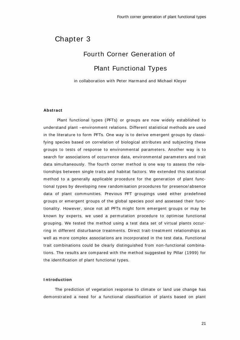
The p-values for the realised niche of plant types composed of the traits
seed number, and spacer length are listed in table 3.5. The plant type without
spacers and low seed number is absent under highly disturbed conditions (Fig-
ure 3.2). Hence its occurrence is positively related to the other treatments
where it occurs. Plant types with only one trait being of medium size occur un-
der highly disturbed conditions with the same frequency as in the other treat-
ments. The method detects no significant difference in the number of occurring
species of these types (p>0.05).
Table 3.5 The realised niche of the PFT is formed based on the traits spacer
length and seed number. Three classes for spacer length (p; 1 = no spacer, 2
= medium spacer length, 3 = long spacer) and three seed number classes (s;
1 = low seed number, 2 = medium seed number, 3 = high seed number) are
permuted to nine PT’s. The values indicate the association (sign), and the sta-
tistical significance (p-values).
Trait classes P-values of relationshipto disturbance regime
Spacer (p) Seed (s) 1 2 3 41 1 0.001 0.001 0.003 -0.0011 2 n.s. n.s. n.s. n.s.1 3 -0.001 -0.001 -0.001 0.0012 1 n.s. n.s. n.s. n.s.2 2 0.001 0.001 0.002 -0.0012 3 n.s. n.s. n.s. n.s.3 1 -0.001 -0.001 -0.004 0.0013 2 n.s. n.s. n.s. n.s.3 3 0.001 0.001 0.003 -0.001
Correlation of dissimilarities
The trait combination plant height, spacer length and seed number
gained the highest Pearson correlation coefficient ρ using the procedure by Pil-
lar (1999) which conforms to the structure incorporated in our test data. It is
followed by the combinations plant height and spacer length and the combina-
tion height, spacer length and colour. The ranking of the ρ-values and the as-
sociated plant traits is listed in table 3.6. Since the trait colour was assigned at
random, we listed means and standard deviations derived from 100 different
test data sets for each trait combination. The ordering in the lower ranks is
highly random, while the first ranks are correctly determined with a high prob-
ability. The single trait colour has the lowest correlation coefficient.

Functional analysis and modelling of vegetation
34
Table 3.6 The optimal trait set is derived with the algorithm by Pillar (1999)
for the test data set. The Pearson correlation coefficient ρ is calculated for the
dissimilarity matrices of the sites by species (squared cord distance) and sites
by the environmental parameters (Euclidian distance). The traits plant height,
spacer length and seed number influence the species occurrence in the test
data set. This combination has the highest correlation coefficient. Trait sets not
including colour are fully deterministic, hence the standard deviation is zero.
The correlation coefficient for single traits except colour can not be calculated,
since for example each different plant height class occurs at least once in each
site, leading to a dissimilarity matrix of sites with only zeros. Using different
trait class classifications did not increase the Pearson correlation coefficients
within our data set.
Pearson ρ Std. Trait combination0.910 0.000 Height, Spacer Length, Seed Number0.809 0.000 Height, Spacer Length0.619 0.011 Height, Spacer Length, Colour0.604 0.000 Height, Seed Number0.598 0.000 Spacer Length, Seed Number0.578 0.006 Height, Spacer Length, Seed Number, Colour0.332 0.013 Height, Seed Number, Colour0.276 0.022 Spacer Length, Seed Number, Colour0.271 0.015 Height, Colour0.062 0.027 Spacer Length, Colour0.060 0.026 Seed Number, Colour0.002 0.030 Colour
Discussion
All trait – disturbance relationships incorporated in the test data set could
be detected using the extended fourth corner method and PFTs were discrimi-
nated. Non-functional traits (colour) were not included in the generated PFTs.
Syndrome versus single trait analysis
After a literature review of life history traits associated with disturbance
and abiotic factors, Marby et al. (2000) concluded, that the importance of
analysing multiple character (e.g. syndromes) instead of single traits was sup-
ported by the wide range of traits thought to be functional by different authors.
Not only the traits thought to be functional differed, but also the relationship
between traits and environmental factors.

Fourth corner generation of plant functional types
35
Jauffret and Lavorel (2003) use a generalised linear model to identify the
attribute response to a factor. Attributes showing a significant response in fre-
quency in one direction of a factor were labelled as ‘decreaser’ or ‘increaser’
according to the direction of the response, or as ‘inconsistent’ if no significant
changes along the gradient could be detected. This procedure would label the
traits seed number and spacer length as ‘inconsistent’ in our test data set, be-
cause the frequency of each state of these traits is similar over the whole dis-
turbance gradient. However, the combination of the traits has a high function-
ality. Whether such complex relationships are relevant for field data or only
occur in our artificial test data set has to be shown by further field work.
A trait effect may even be reversed depending on another trait attribute.
While the occurrence of PTs with either high seed number or long spacers, are
positively related to highly disturbed treatments, the combination of both trait
states is disadvantageous (Figure 3.2, Table 3.5). Forming PFTs only from sin-
gle trait analysis would not produce a valid PT factor relationship in this case.
Another issue in forming PFTs by single trait analysis is to assure that the
trait states co-occur in the species, likewise it is done by Jauffret and Lavorel
(2003). All PTs identified by the proposed method comprise species since our
null model only randomises the observed data. The necessity of analysing syn-
dromes instead of combining single trait analysis was also found by Marby et
al. (2000) who analysed species level distribution of traits in a temperate
woodland flora and associated the environmental conditions with different
groups of traits which tend not to co-occur within species.
Null models
To identify co-occurring PFTs in a given treatment we used the ‘lottery’
model (Sale 1978). It hypothesizes a founder controlled community with no
differences in competitive ability between species. The alternative hypothesis
to this model is that species belonging to certain plant types perform better
than others. Using the model without correction assigns -on average- the same
number of species to each plant type. It therefore evaluates whether the ob-
served plant types occur proportional to the number of species they cover.
However, if total species number per plant type is of concern, normalising
group sizes assumes not the occurrence probabilities of single species but the
expected number of species per group to be equal. The alternative hypothesis
is that there are some PTs which were observed more frequently than others.

Functional analysis and modelling of vegetation
36
The frequency of occurrences indicates which PT will dominate within a treat-
ment.
If not PFT composition per treatment (community analysis) but occur-
rence of a PFT across treatments (niche analysis) is concerned, a different null
model is required. The environmental control model (Whittaker 1956) as used
by Legendre et al. (1997) assumes species occurrence to be independent of
environmental factors. The alternative hypothesis is that a given species is
confined to appropriate environmental conditions. While the number of obser-
vations of each species (rarity) is seen as a constraint, no interactions between
species (e.g. competition, mutualism) are assumed. If the species diversity
differs between sites of different environmental conditions, the method is bi-
ased to overestimate the frequencies of species that tend to occur at species
rich sites in the observation and vice versa. Hence, we decided to use a null
model with fixed row and column sums to fix species rarity and diversity per
site.
The test data set incorporates only one environmental gradient. However,
various gradients may influence the species composition simultaneously. To
incorporate several environmental factors, each factor needs to be classified
into discrete classes and each site has to be assigned to a combination of fac-
tor classes (treatments). The ability to correctly discriminate PFTs (Type I er-
ror) is strongly influenced by the number of sites and the number of traits used
to compose the PFTs. Increasing the amount of sites may allow to incorporate
more traits into PFT generation.
Comparison with other approaches
Our method advances the fourth corner method developed by Legendre
et al. (1997). The original method focuses on a test of the global relationships
between single traits and environmental factors, less on testing each possible
combination of traits. A second branch in the three-table joint analysis is based
on correspondence analysis and include the RLQ technique (Doledec et al.
1996; Ribera et al. 2001) or consecutive multivariate techniques (McIntyre &
Lavorel 2001). A third branch resides in the framework of Generalised Linear
Modelling and logistic regression techniques (Kleyer 1999a; Jauffret & Lavorel
2003). Among these techniques, the approach probably most similar to ours is
of Nygaard & Ejrnæs (2004) who start with an a priori classification of func-
tional groups with classification trees. Subsequently, they also use an inflated

Fourth corner generation of plant functional types
37
matrix (‘list file’) based on Legendre et al. (1997) and proceed with Analysis of
Variance using cross-validation to assess generality of their models. Similar to
Legendre et al. (1997), they only test a global relation of functional types with
treatments which restricts understanding the contribution of individual trait
combinations to plant – environment relations. The latter can be achieved by
optimisation methods as presented in our approach or by Pillar (1999; 2003).
Moreover, we consider null models as a straightforward method to cope with
lack of independence between observations in an inflated matrix.
The results of the optimisation procedure by Pillar (1999) are valid for the
test data set and contingent with the results of our extended fourth corner
method. However, it detects the functional traits, not the direction of the asso-
ciation to the environmental parameters, or their significance. His algorithm
will deliver a trait ranking, even if none is functional, while our method tests
the significance of association for each PT to each environmental factor. Pillar
(2003) enhanced his method by using a cluster analysis to find the optimal
trait classes of the PTs. However, he still uses the correlation of dissimilarities
to discriminate the optimal trait set, hence the results concerning our data set
would be similar.
Perspective
If several traits influence the occurrence of a species, they can be ex-
pected to differ in their importance. If the data set comprises species differing
sufficiently in their trait attributes, the trait hierarchy can be inferred as de-
scribed in the results section.
The presented null models are based on presence / absence data, be-
cause this is the most common data format. Using abundance data can im-
prove such an analysis (Gotelli et al. 1987). This extension can be done by de-
signing a new null model which suits this kind of data.
The results of the presented method can readily be used to build scenar-
ios of future vegetation development. Applying the ‘lottery ’ model and pro-
jecting the derived PFT- environmental conditions relationships on a hypotheti-
cal map of site conditions (incorporating climate or land use change) results in
a map of communities of plant functional types. The uncorrected p-values of

Functional analysis and modelling of vegetation
38
the ‘lottery’ model compare the probability of occurrence of each species of the
PFT compared to a total occurrence probability in the whole data set. Projecting
these values on a map of site conditions displays the relative habitat suitability.
Likewise it is done with multiple regressions (GLM) for single species (Guisan &
Zimmermann 2000). Hence, these projections may be used for predictive
habitat distribution modelling of PFTs.

Part II:
Modelling of PFTs
a mechanistic model


Trait hierarchies and sequence effects
41
Chapter 4
Trait hierarchies and sequence effects in simulated community assembly using the
leaf-height-seed plant ecology strategy scheme
in collaboration with Michael Kleyer
Abstract
Several sets of traits are suggested to establish plant functional types.
While extensive analyses of experimental data are made to select traits that
predict the response of plants to environmental factors, few studies use a
simulation approach to predict suites of functional traits. This paper focuses on
the trait set suggested by Mark Westoby (1998): specific leaf area (SLA), plant
height and seed mass. We simulated the assemblage of plant types on a gradi-
ent of fertility and disturbance and assessed the functionality of the suggested
traits. We also characterised how invasibility depends on disturbance and fer-
tility. We present the results of a spatially explicit simulation using
LEGOMODEL, an individual based, ecological field model. The competitive su-
perior trait states as well as the functional hierarchy change between different
treatments. Plant height always determines competitive success, while seed
mass is more relevant for survival than SLA at fertile sites and vice versa at
infertile sites. High fertility as well as low disturbance leads to low diversity of
functional types. The invasibility of a plant community depends on the combi-
nation of fertility and disturbance. Communities characterised by strong com-
petitors show a strong resistibility even in the absence of the best fitted plant
type.
Introduction
On the community and landscape scale, plant functional response to en-
vironmental change is often studied by analysing the composition of plant traits
across communities. This is done under the premise that suites of morphologi-
cal and physiological traits represent adaptive responses to environmental con-
ditions (Stebbins 1974; McIntyre et al. 1999). Traits are correlates to basic life
history processes such as photosynthesis or demographic survival rates that
are hard to quantify for larger species pools (Garnier 1997). Trait-based func

Functional analysis and modelling of vegetation
42
tional responses to environmental factors were demonstrated in observational,
experimental, and long-term permanent plot studies (Fernandez et al. 1993;
Kleyer 1999a; McIntyre et al. 1999; Fonseca et al. 2000; Craine et al. 2001;
Jauffret & Lavorel 2003), and also across contrasting landscapes (Kleyer 2002).
Although functions such as persistence, expansion, generative reproduc-
tion, vegetative regeneration and dispersal all are necessary for the long-term
survival of plant populations, it is unlikely that all of these functions share
similar relevance across all possible environments. We expect that e.g. habitat
qualities stable in space and time will require a more consistent response in
persistence traits than in dispersal or regenerative traits (Grime et al. 1988;
Shipley et al. 1989; Diaz & Cabido 1997). On the other hand, habitats with
frequent and severe disturbance impacts may require a more consistent re-
sponse in dispersal and regenerative traits than in persistence traits. In any
given environment, a certain hierarchy in principal response functions such as
persistence, regeneration and dispersability can be expected. On large envi-
ronmental gradients, we expect a turnover of such functional hierarchies. The
extent of this turn-over, the interplay and the trade-offs between response
functions on environmental gradients appear to be largely unknown. Up to
now, most authors have concentrated on the specific plant traits that contrib-
ute to just one or two of these principal functions. For instance, traits such as
canopy height, leaf size, mass and lifespan, branching, woodiness, sclero-
phylly, stem and leaf dry matter content all contribute to the vertical expansion
of plants and their capacity to acquire carbon. Several studies have addressed
the relative importance of such traits for a single function such as carbon gain
across several environments (e.g. Wright & Westoby 2003). In this context, a
distinction is necessary between genetic or ‘primary’ trade-offs among traits
and ‘secondary’ environment – enforced trade-offs (Westoby et al. 2002; Sud-
ing et al. 2003). Primary trade-offs (e.g. leaf life span - specific leaf area, seed
size - seed number) result in strong correlation (Westoby et al. 2002) and their
evolution may also be analysed in terms of hierarchies (Worley et al. 2003).
Secondary trade-offs (e.g. high above-ground disturbance frequency favours
low height and high vegetative regeneration) are in the focus of trait hierar-
chies as presented here, and need to be discussed in their interaction with pri-
mary trade-offs.

Trait hierarchies and sequence effects
43
To determine hierarchies, trait composition of community or landscape
species pools has to be analysed in relation to the environmental factors or
gradients that structure them. For large species numbers, ‘soft’ traits such as
seed number, plant height etc. can be more easily identified from measure-
ments (Cornelissen et al. 2003) or databases (Knevel et al. 2003) than ‘hard’
traits with demonstrated links to plant function (e.g. demographic survival
rates, carbon gain, Diaz et al. 1999). Consistency of trait states among species
ordered along environmental gradients can then be seen as an indicator for
trait hierarchies (Kleyer 2002).
The term hierarchy has been frequently used in the context of competi-
tion, where it denotes competitive superiority of species measured against e.g.
a phytometer (Keddy et al. 2002) or as growth of a target species in pairwise
mixture relative to growth of target in monoculture (Wilson & Keddy 1986;
Miller & Werner 1987; Shipley 1993). Several studies also analyse the variation
of life history traits in competitive hierarchies (Walck et al. 1999; Howard &
Goldberg 2001; Keddy et al. 2002). Competitive hierarchies rank the perform-
ance of species in assuming that ranks are the outcome of a single process, i.e.
competition among species. Trait hierarchies rank consistency of trait states
across species pools, based on species performance. They show which traits
are most functional for occurrence / survival. No a priori reference is made to
processes such as competition, colonisation, or stress tolerance, although trait
states can be interpreted as biological correlates to plant functions as persis-
tence, regeneration or dispersability. A concept related to trait hierarchy turn-
over is that of rank reversals of a single trait driving rank reversals of the rela-
tive fitness of species. This was elaborated in the framework of coexistence
theory (Chesson 1985; Kitajima & Bolker 2003). An example for a key trait in
this context is Relative Growth Rate (RGR) in relation to light gradients (Sack &
Grubb 2001).
Trait hierarchies order the relevance of plant traits for survival, an ap-
proach that is preceded by plant strategy concepts. Among the many concep-
tual strategy schemes that have been proposed (e. g.Van Valen 1971; Gadgil &
Solbrig 1972; Whittaker & Goodman 1979) the C-S-R triangle of Grime (1974;
1979) has received special attention in plant ecology. A challenge to all these
strategy schemes still is to clearly characterise the sets of biological attributes
that make up the elements of a certain strategy and enumerate the species
that can be assigned to the strategy (Hodgson et al. 1999). These shortcom

Functional analysis and modelling of vegetation
44
ings have motivated Westoby (1998) to propose a simple strategy scheme
composed of three quantifiable traits. The traits are specific leaf area (SLA),
plant height, and seed mass. The position of a species within the three-
dimensional space of the axes SLA, height and seed mass may be regarded as
a representation of ability to persist in its habitat or to colonise distant habi-
tats. Specific leaf area is correlated with relative growth rate (Garnier 1997;
Wright & Westoby 1999) and thus related to competitive ability, together with
plant height (Gaudet 1988; Tilman 1988). Seed weight is associated with dis-
persal, establishment, and seed bank longevity (Bekker et al. 1998; Thompson
1998; Kidson & Westoby 2000).
The charm of the LHS scheme is simplicity. Its applicability, however, de-
pends on whether the three traits capture enough plant variability to function-
ally represent the floristic diversity along major environmental gradients such
as fertility, disturbance, and fragmentation. This can only be tested if predic-
tions are available regarding the success of plant types composed of combina-
tions of the three traits in different environments.
In this paper we use a simulation approach to predict LHS combinations
for different disturbance regimes on soils with low and high fertility. We are
interested in combinations of the three traits SLA, plant height and seed size
that perform best in the simulated environments and in a hierarchy of these
traits across different environments. We ask whether all three traits are equally
functional for survival in all environments (no hierarchy), whether there is a
superior trait across all environments (constant hierarchy), or, whether differ-
ent traits are functional for certain environments (environment-driven hierar-
chy)?
We also use the LHS scheme to simulate the invasion of a superior plant
type. Invasive species are able to alter the resident community structure or
even drive other species to extinction (Mooney & Drake 1986). To understand
biological invasions, it is necessary to investigate the effect of external and
internal factors which influence the susceptibility of natural ecological commu-
nities to invasiveness. Several factors have been shown to affect the invasibil-
ity of communities. These are vegetation composition (Van der Putten et al.
2000), disturbance regime (Burke 1996), the amounts of unused resources
present (Davis et al. 2000) as well as species richness (Elton 1958). While
studies based on observed patterns in the field found either positive or neutral
relationships between diversity and invasibility (Lonsdale 1999; Van der Putten

Trait hierarchies and sequence effects
45
et al. 2000), theoretical considerations (Elton 1958) supported by experimental
evidence argue for a negative relationship between species diversity of resident
communities and invasiveness (Knops et al. 1999; Naeem et al. 2000; but see
Wardle 2001). Inconsistent results were found concerning the contribution of
traits to invasiveness of (exotic) species or community invasibility. In a large-
scale observational study, the local and regional abundance of ca. 400 exotic
species on Mediterranean islands did correlate less to plant traits than to bio-
geographical origin (Lloret et al. 2004). In experiments, invasiveness corre-
lated to plant traits and invasibility to resource availability (Milbau et al. 2003)
or standing biomass (Troumbis et al. 2002). Trait composition of successful
invaders may change during a successional series (Thompson et al. 2001).
In the context of this study, the extent to which sequence effects alter
trait hierarchies shows the impact of sequence effect vs. environmental factors
on community assembly.
The LHS scheme may provide a suitable reduction of traits to construct
simple resident communities of plant types whose LHS composition can be
compared to that of the invader.
Methods
The model
We used LEGOMODEL (Kleyer 1999b), an individual based, ecological
field model (Wu et al. 1985; Czaran 1998). It simulates populations of plant
types that occupy space to extract resources for growth and regeneration.
Plant types originate from simple building rules, able to express different trait
attributes according to the specific initialisation of the plant type. The resulting
architecture of each plant is predefined by the building rules but also influenced
by its local environment including interaction with other plants. The simulation
starts with randomly dispersed seeds, germinating in the next time step. A
growing plant consists of different modules: stem, leaves, roots, and stolons or
seeds for regeneration (Figure 4.1). The plant extracts the resources needed
for further growth and regeneration according to the area of light exposed
leaves and the soil volume penetrated by its roots. A proportion of the assimi-
late a ramet of a clonal individual has gained is pooled among the system of
connected ramets and redistributed to all ramets (clonal integration).

Functional analysis and modelling of vegetation
46
Figure 4.1 Typical growth of a tall plant in LEGOMODEL. The gained resources
are distributed between the mother plant and the two ramets (right and left).
The plants consist of the modules stem, leaves, spacer, roots or seeds.
Figure 4.2 Ecological fields incorporated in LEGOMODEL. Below each leaf a
directed light depletion zone and around each root cell a soil resource depletion
zone is formed. Resource depletion zones are growth barriers for other plants.

Trait hierarchies and sequence effects
47
Leaves and roots of the virtual plant generate resource depletion zones
(Figure. 4.2). Resource depletion zones are growth barriers for other plants.
Shaded leaves produce no assimilate but still respire, hence consume assimi-
late in every time step. Plant growth is externally inhibited by adjacent re-
source depletion zones, or internally by lack of assimilate which is consumed
by respiration. The resources available to an individual plant depend on the
distance from adjacent depletion zones. The energy gain of every time step is
calculated as follows (see Tilman 1988):
∑ •−=plant
modulegaingaingain nrespiratiomodulecesoilresourlightE )(),min( (6)
Shaded seeds are dormant until light reaches the surface, either due to
disturbance or senescence of the shading plant. Seed dormancy is limited to
one year and maximum plant age is set to six years. Except plant height, spe-
cific leaf area and seed size and correlated attributes (see below), all other trait
parameters in LEGOMODEL were kept constant.
To simulate the LHS traits, we incorporated the following trade-offs:
• Plant types with low SLA require more assimilate to build up leaf tissue
than plants with low SLA (construction costs SLA high / low = 1 / 1.6),
which in turn leads to a lower growth-rate (Garnier 1997; Wright & Wes-
toby 1999). These plants are subsequently able to conserve assimilate
more effectively by making a better use of the same amount of extracted
soil resources.
• Seed mass is correlated with the amount of assimilate needed for seed pro-
duction. The same amount of energy may produce fewer, but bigger seeds
or more, but smaller seeds (Kidson & Westoby 2000). Big seeds provide
more assimilate to the seedling than small ones.
• Plant height is correlated with leaf area and root length to provide a con-
stant root/shoot ratio.
The model is designed to simulate the course of succession of the plant
type assemblage according to disturbance and soil resource supply. Distur-
bance is incorporated by cutting of all plant parts higher than 10 cm. Soil fer-
tility influences the efficiency of the root modules in extracting resources. All
resource depletion zones around a root or below a leaf cell are removed once
the plant part is removed, due to disturbance or senescence.

Functional analysis and modelling of vegetation
48
Simulation Szenarios
We simulated six treatments, i.e. monthly cutting, yearly cutting, and
cutting once every nine years on soils of low and high fertility. The traits of the
LHS scheme were simulated with two states, i.e. low vs. high specific leaf area,
low vs. high plant height and low vs. high seed weight. Hence, 23 = 8 plant
types took part in the study (Table 4.1). We started by initialising 20 seeds of
each plant type randomly dispersed over an empty site of a size equally to 4
m². The assembly trajectories of the developing communities are recorded
over a time period of 100 years with 400 replications.
Table 4.1 Trait state attributes of the plant types incorporated in LEGOMODEL.
The relative differences between trait state high and low are 1.6 for SLA, 3 for
height and 2 for seed mass.
Plan type SLA Height Seed Mass1 low high high2 low high low3 low low high4 low low low5 high high high6 high high low7 high low high8 high low low
A survivorship analysis for censored data assessed the success of the
various plant types. We ranked the performance of all plant types for each
treatment by comparing their survival times across all repetitions. Cox F-Test
for singly censored data (Lee 1980) was used to test for differences between
survivorship of two plant types, for an example calculation see Appendix A.4.2.
If a plant type displayed a significantly higher survivorship than another plant
type, it received a higher rank. If differences between two plant types were not
significant, both plant types got the same rank. A detailed description together
with an example is given in the Appendix A.4.1. From the results, we took the
type with the highest survival rate to further study sequence effects. In these
runs, this type was initialised after 20 years of simulation time, when the re-
maining plant types already assembled to communities. The runs then carried
on for another 100 years.

Trait hierarchies and sequence effects
49
Trait hierarchy
The hierarchy of traits is based on the consistency of trait states (high vs.
low) across the ranking of the surviving plant types. For instance, if two plant
types are on the first rank and both are of small height and high SLA while
seed mass differs in its state, than plant height and SLA are more functional
than seed weight. If the second rank is occupied by a plant type having also
small height but low SLA, the resulting hierarchy will be: plant height > SLA >
seed weight. As the eight plant types represent a complete permutation of the
three LHS traits, we could build the hierarchy by analysing the variance of the
trait states across the ranks for each treatment separately. For each trait, we
counted the number of ranks (from the first rank on downwards) for which the
corresponding state remained constant. The higher the number, the higher is
the position of the trait in the functional hierarchy.
Sequence effects
To analyse the resistance of the plant assemblages to invasions, the dif-
ferences in the survival rates between synchronous and asynchronous (delay of
the dominant type) initialisation of the plant types were compared across
treatments. The differences are given as a percentage of decrease in survival
over 100 years under delayed initialisation compared to synchronous initialisa-
tion. A one-tailed test of differences of percentages (Sachs 1992) was per-
formed.
Results
At high fertility and low or medium disturbance intensity, the assembly is de-
terministic and of low diversity. Two plant types exclude all other types after
80 years (Figure 4.3). The type with highest rank has high SLA, height and
seed mass, while the second has high height and seed mass, but low SLA. If
fertility is low, the type with low height, SLA and seed mass is always at the
first rank, regardless of the disturbance level. In these treatments, the com-
munity assembly is more stochastic (i.e. none of the plant types attains 100 %
survivorship) and of higher diversity. If highly disturbed, plant types at the first
rank (plant type 4 & 7) are small, with high SLA and a high seed weight under
fertile conditions and low SLA and low seed mass under infertile conditions. The
ranking for medium disturbed and rarely disturbed sites are similar at fertile as
well as at infertile sites, although the differences between the types are some

Figure 4.3 Survival curves of eight plant types simulated over 100 years in sixtreatments. The traits of the plant types are listed in table 4.1.
Survival of plant typesTreatment: fertile, medium disturbed
Sur
vival
rate
Years
Survival of plant typesTreatment: fertile, highly disturbed
Sur
vival
rate
Years
Survival of plant typesTreatment: fertile, rarely disturbed
Sur
vival
rate
Years
Survival of plant typesTreatmen: infertile, rarely disturbed
Sur
vival
rate
Years
Survival of plant typesTreatment: infertile, medium disturbed
Years
Sur
vival
rate
Survival of plant typesTreatment: infertile, highly disturbed
Years
Sur
vival
rate
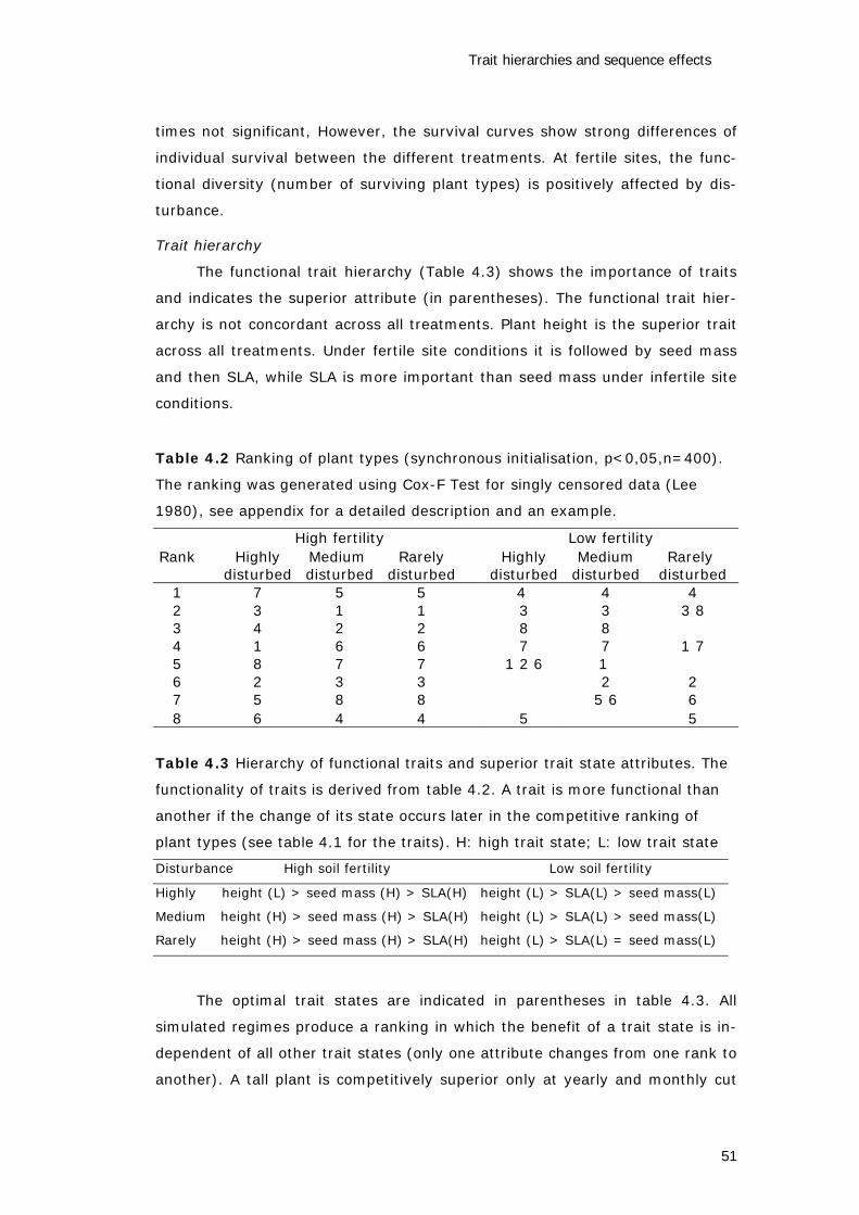
Trait hierarchies and sequence effects
51
times not significant, However, the survival curves show strong differences of
individual survival between the different treatments. At fertile sites, the func-
tional diversity (number of surviving plant types) is positively affected by dis-
turbance.
Trait hierarchy
The functional trait hierarchy (Table 4.3) shows the importance of traits
and indicates the superior attribute (in parentheses). The functional trait hier-
archy is not concordant across all treatments. Plant height is the superior trait
across all treatments. Under fertile site conditions it is followed by seed mass
and then SLA, while SLA is more important than seed mass under infertile site
conditions.
Table 4.2 Ranking of plant types (synchronous initialisation, p<0,05,n=400).
The ranking was generated using Cox-F Test for singly censored data (Lee
1980), see appendix for a detailed description and an example.
High fertility Low fertilityRank Highly
disturbedMedium disturbed
Rarelydisturbed
Highlydisturbed
Mediumdisturbed
Rarely disturbed
1 7 5 5 4 4 42 3 1 1 3 3 3 83 4 2 2 8 84 1 6 6 7 7 1 75 8 7 7 1 2 6 1 6 2 3 3 2 27 5 8 8 5 6 68 6 4 4 5 5
Table 4.3 Hierarchy of functional traits and superior trait state attributes. The
functionality of traits is derived from table 4.2. A trait is more functional than
another if the change of its state occurs later in the competitive ranking of
plant types (see table 4.1 for the traits). H: high trait state; L: low trait state
Disturbance High soil fertility Low soil fertility
Highly height (L) > seed mass (H) > SLA(H) height (L) > SLA(L) > seed mass(L)
Medium height (H) > seed mass (H) > SLA(H) height (L) > SLA(L) > seed mass(L)
Rarely height (H) > seed mass (H) > SLA(H) height (L) > SLA(L) = seed mass(L)
The optimal trait states are indicated in parentheses in table 4.3. All
simulated regimes produce a ranking in which the benefit of a trait state is in-
dependent of all other trait states (only one attribute changes from one rank to
another). A tall plant is competitively superior only at yearly and monthly cut

Functional analysis and modelling of vegetation
52
ting regimes on fertile soil. On all other regimes small plants are superior. High
SLA and seed mass are advantageous at high fertility levels, while low SLA and
low seed weight are superior at low soil fertility. This difference is not signifi-
cant at rarely disturbed sites with low soil fertility.
Invasion resistance
We simulated sequence effects by a delayed initialisation of the plant
type that was most successful in the previous simulations. For each treatment,
the community is assembled from the less successful plant types during the
first 20 years, then the delayed plant type enters the community and the as-
sembly carries on for another 100 years. The decrease in survival of this plant
type from synchronous to asynchronous initialisation is given in table 4.4. Ex-
cept for the intermediately disturbed treatment on infertile soil, delayed enter-
ing leads to a decrease in survival. At high fertility, decreasing disturbance in-
tensity increases the resistance against the invader, i.e. survival of the for-
merly successful plant type is suppressed more in the less disturbed commu-
nity. At infertile sites, invasion resistance of the most frequently disturbed sites
is higher than on rarely disturbed sites, followed by medium disturbed sites
with even slightly better survival chances after delayed initialisation.
Table 4.4 Invasiveness of the most successful plant type
Decrease in survival after 100 years due to a delay of 20 years in initialisation.
A one-sided z test of differences between percentages (Sachs 1992) proved all
differences to be significant (p=0.05, n=400). ** = p<0.01.
High soil fertility Low soil fertility Effect ofTreatment Type Percentage Type Percentage fertility
Highly disturbed 7 41% 4 76% - (**)Medium disturbed 5 60% 4 -9% + (**)Rarely disturbed 5 86% 4 45% + (**)
At equal disturbance intensity, an increase in fertility leads to a decrease
of invader success except for the most frequently disturbed sites (Table 4.4).

Trait hierarchies and sequence effects
53
Discussion
We tested the suitability of the LHS scheme for a virtual plant assem-
blage across several treatments and assessed the effects of a delayed arrival of
plant types in an established assemblage.
Our model is individual based and simulates community assembly on a
single patch. LEGOMODEL includes:
• soil resources and disturbance intensity as major environmental con-
straints,
• trade-offs in allocation to plant height, leaf mass and size, and seed weight
that translate in building rules for plant types,
• spatially explicit competition limited to neighbouring plants, based on local
resource depletion zones (ecological fields).
It therefore meets the requirements for predictive ecological theory as
formulated by Silander and Pacala (1990) and Tilman (1990). Recent modelling
approaches emphasise the value of spatially explicit competition mechanisms
based on ecological fields or ‘fields of neighbourhood’ (Berger & Hildenbrandt
2000) which depart from the mean field assumption (Law et al. 2000).
Other modelling approaches also use suites of morphological and regen-
erative traits to simulate the assembly of communities. A classical model is the
Vital Attributes model from Noble & Slatyer (1980) with several derivates
(Moore & Noble 1990; Lavorel 2001).
Mustard et al. (2003) used a simulation approach in which the parameter
combinations of plant types were able to evolve over several generations.
Similar to our results, fertile sites with low disturbance were character-
ised by tall plants with medium SLA. Likewise, a second type with medium
height and a high SLA occurred mainly at high disturbance levels. LEGOMODEL
exhibits major differences to the model of Mustard et al. (2003) only in case of
SLA under infertile conditions. Here, we predict low SLA which is in line with
empirical studies (Poorter & De Jong 1999; Fonseca et al. 2000). Seed weight
is not modelled by Mustard et al. (2003).
Height
Across all treatments, plant height is the superior trait. At high fertility,
seed mass is more consistent than SLA, while SLA is more consistent than seed

Functional analysis and modelling of vegetation
54
mass at low fertility. Different disturbance treatments do not alter the ranking
of the traits themselves, they only alter the trait states, i.e. the states of height
and seed mass shift from ‘high’ to ‘low’ in frequently disturbed treatments.
Plant height reflects investment in supportive structures necessary for
space utilisation. In our model, leaves assimilate and respire while stems only
respire. Each increment in vertical growth requires a positive balance of as-
similation and respiration in the previous time step and implies construction
costs. After reaching height at maturity, assimilation and respiration continue
and investment in construction is finished. Growth also requires sufficient soil
resources. Thus, plant types are favoured that allocate less to support struc-
ture at infertile treatments. If the return interval between disturbance impacts
and removal of biomass is short, small plant height is superior even on fertile
sites, because investments in construction until height at maturity are shorter
and assimilation can pay off into seed production earlier. Our modelling results
concerning height in relation to disturbance and fertility are in line with earlier
models (Tilman 1988). Fernandez et al. (1993) showed in a study of Mediter-
ranean grasslands that the relative abundance of species with different attrib-
utes varies with the level of stress (water and nutrient availability) and distur-
bance (grazing and ploughing) concluding that “the main trend in variation is
related to plant size“. Walck et al. (1999) found the competitive hierarchy also
closely related to plant size in an experiment.
Seed mass
Our model includes the seed mass – seed number trade-off as seed num-
ber is assimilate gained divided by seed mass. If the seed mass is small, more
seeds are produced. In the absence of any hazard, smaller seeds should be
advantageous for population increase. However, in an environment with abun-
dant light and resource depletion zones, a larger seed mass conveys more re-
serves to the establishing seedling. If the first leaf of a seedling is growing into
a light depletion zone, larger seed reserves make the formation of a second
leaf possible, probably outside of a depletion zone, even if the balance of as-
similation and respiration of the first leaf is negative. Growing empirical evi-
dence supports the seed mass -- seed number trade-off in plants (Turnbull et
al. 1999; Jakobsson & Eriksson 2000) and the functional importance of larger
seed mass when the seedling encounters hazards such as deep shade or inter-
specific competition from other seedlings (Westoby et al. 2002). Effects of seed
size on competitive ability in sand dunes are also found by Rees (1995).

Trait hierarchies and sequence effects
55
Leishman (2001) experimentally showed under fertile undisturbed conditions,
that there is a “competitive hierarchy among species based on seed size where
larger seeded species beat smaller seeded species”.
SLA
Specific leaf area or its inverse, Leaf Mass Area, has been regarded as a
useful indicator of leaf strategy (Westoby et al. 2002), because it reflects
physical strength of the leaf and is correlated with relative growth (Westoby
1998), which in turn is correlated with productivity or fertility (Poorter 1989).
Strong negative correlations of SLA were also found to leaf lifespan (review in
Westoby et al. 2002) and photosynthetic capacity of leaves (Reich et al. 1999).
Construction costs tend to be similar among leaves with high and low SLA
(Poorter & De Jong 1999). Longer life-span of leaves with lower SLA permits
conservation of acquired resources (Eckstein et al. 1999; Aerts & Chapin 2000;
Westoby et al. 2002). This may be especially true for habitats not character-
ised by frequent disturbance impacts (e.g. mowing, Ryser & Urbas 2000).
Corresponding to our results, several studies found species with low SLA
more likely to occur on sites with low fertility or rainfalls and those with high
SLA on sites with high fertility or rainfall (Poorter & De Jong 1999; Fonseca et
al. 2000). In LEGOMODEL, SLA was implemented based on the simplifying as-
sumption that leaves with low SLA require more assimilate for growth, while
resource conservation at maturity would be higher with low SLA.
As an effect of the different assimilate requirements, the relative growth
rate is proportional to SLA as found by Westoby (1998).
Trait hierarchy
Although high SLA is a relevant trait for rapid growth and effective space
utilisation, our model predicts that high seed mass is more important than high
SLA under fertile conditions. This hierarchy is reversed under infertile condi-
tions. Is there any empirical evidence for this prediction? We know of only one
observational study that directly applied the LHS scheme (Lavergne et al.
2003). However, the authors did not use disturbance and fertility as explana-
tory environmental factors. A study of Landsberg et al. (1999) showed a strong
association of canopy height to grazing response, while the association of SLA
and seed size was variable. A recent meta-analysis of species response to
grazing in Australian dry shrublands and woodlands did not find any significant
relation with traits including height, SLA, and seed size (Vesk et al. 2004).

Functional analysis and modelling of vegetation
56
Other studies may include also more than the three traits of the LHS scheme,
but often one of the three traits is missing. This makes it difficult to compare
the functional hierarchy found in our model to the results of such studies. Diaz
et al. (2001) found that height was the best single predictor for grazing re-
sponse, while SLA had only a small predictive value. Seed mass was not in-
cluded. On a disturbance / fertility gradient plane, Kleyer (1999a; 2002) found
that height was the most consistent trait, while regenerative traits such as
seed size contribute to alternative pathways of occurrence / survival at a single
combination of disturbance intensity and fertility. In these studies, SLA was not
included.
Our simulated trait hierarchies remain invariant to disturbance regimes
within each fertility treatment but change across fertility treatments. Keddy et
al. (2000; 2002) argued that competitive hierarchies are relatively independent
of the environment, i.e. rank reversals are not to be expected if the environ-
ment shifts from high to low fertility. This has relevance for trait hierarchies,
because similar to competitive hierarchies between species, it is the plant per-
formance (or plant type performance in our simulations) that is measured. In
their competition experiments, Keddy et al. (2000; 2002) recorded the percent
reduction in biomass of a ‘phytometer’ species grown together with a test spe-
cies under two fertility regimes. According to the data, this phytometer must
have been a very weak competitor because almost all test species reduced its
biomass in both the high and low fertility treatments. They found that the rela-
tive competitive performances of the test species are similar at high and low
fertility. However, if the phytometer species is the weakest competitor in the
whole species set, reduced nutrient fertility will confer no competitive advan-
tage to this species. On the other hand, if a phytometer with a more moderate
competitive ability had been grown together with test species exhibiting a
range of high to low competitive abilities, then rank reversals between high
and low fertility treatments would have been more probable.
Diversity
Our simulations show that diversity interacts with both fertility and dis-
turbance. It decreases with increasing fertility and decreasing disturbance.
However, it also decreases at high disturbance and low fertility. This result is
consistent with a combination of the humped-back model (Grime 1974) and
the Intermediate Disturbance Hypothesis (Huston 1979). In these concepts,
dominant species competitively exclude other species if dominance is not bro

Trait hierarchies and sequence effects
57
ken by either stress at low fertility levels or by disturbance. On the other hand,
many species are unable to regenerate at high levels of either stress or distur-
bance. At intermediate disturbance or stress levels, plant species diversity is
supposed to be maximised (Grime 1973; Connell 1978; Huston 1979). There is
growing empirical evidence for both concepts with respect to species diversity
(Goldberg & Miller 1990; Grace 1999; Gough et al. 2000; Shea et al. 2004)
and diversity of functional groups (Kleyer 1999a, 2002).
Sequence effects
Sequence effects represent a test for the stability of a trait hierarchy.
Stable trait hierarchies should show resilience to delayed entering in the as-
sembly process, in particular if the invader is the formerly superior plant type.
This means the invader should regain its former position in the rank order of
survivorship. Our results show that invader success increases with disturbance
under fertile conditions. It peaks at intermediate disturbance if fertility is low.
Note that height remains the first order trait and only the third order trait (SLA
or seed mass) is reversed in the hierarchy, if sequence effects appear (data not
shown). This suggests that the underlying model is that of a change from
founder control and inhibition at the high fertility / low disturbance corner to
increasing redistribution of competitive interactions at the intermediate distur-
bance / low fertility corner (Connell & Slatyer 1977). Disturbance and stress
play an important role in breaking established founder control. Release from
competitive interactions provides higher chances of establishment for the in-
vader and thus higher invasibility of the resident community.
In our model, deterministic assemblies with low diversity exhibit higher
sequence effects than more stochastic assemblies. Likewise, the trait hierarchy
is more stable if the assembly is more stochastic and diverse. While experi-
mental studies (Robinson & Edgemon 1988) as well as theory (Elton 1958)
suggest a negative association between biological diversity and invasibility, due
to increased competition in species rich communities, most observational field
studies find no support for such a negative association (e.g. Naeem et al. 2000
and references therein). Moore et al. (2001) emphasise that species-poor
communities can be more saturated than species-rich communities. This de-
pends on the size of the community species pool (Partel et al. 1996; Grace
1999) which is small when either abundant resources enable dominance or
high disturbance excludes species with low regeneration (Shea et al. 2004).
Co-variation of extrinsic factors such as fertility and disturbance controlling

Functional analysis and modelling of vegetation
58
invader success has been stressed by Naeem et al. (2000) as “the most likely
explanation” for the conflicting results between experimental and observational
studies. According to Moore et al. (2001), a negative relationship between
richness and invasibility is likely in systems where recruitment is limited. This
is not the case in our single patch simulations in which all plant types have
equal chances for recruitment.
Our simulation experiment supports the observational results by Robin-
son et al. (1995) and Wiser et al. (1998) that invasibility is positively related to
functional diversity, as long as the resident functional diversity results from
extrinsic factors. The simulation result that invasibility is positively affected by
disturbance under fertile conditions was also experimentally found by Crawley
et al. (1999).
Limitations of the LHS strategy scheme
Life history features as life cycle, aerenchyma, clonal growth, position of
regenerative buds, and seed appendices in relation to dispersal agents were
not included in the LHS scheme (Westoby 1998). There is evidence that more
than the LHS traits are relevant for plant strategies (Poschlod et al. 2000). For
instance, the position of regenerative buds can be essential for discriminating
perennial plant types surviving under below-ground disturbance regimes (e.g.
tilling) versus above-ground regimes (e.g. mowing, Kleyer 1999a; Sparrow &
Bellingham 2001; Klimesova & Klimes 2003). To account for this shortcoming
of the LHS scheme, we only modelled above-ground disturbance. On the other
hand, our simulations show that no LHS trait is negligible within our template
of disturbance / fertility regimes.
LEGOMODEL has produced hypotheses on the hierarchy of plant traits
during assembly of plant communities that correspond to empirical results. We
provide predictions of LHS trait combinations for certain fertility / disturbance
regimes. The wider applicability of the LHS scheme has to be demonstrated by
further field work.

Sensitivity of LEGOMODEL
59
Box 1
Viability of plant trait combinations:The sensitivity of LEGOMODEL an
individual based ecological field model
Abstract
A sensitivity analysis of LEGOMODEL is performed. A factorial design is
carried out for the plant traits incorporated in the Leaf-Height-Seed scheme for
different fertility and disturbance regimes. The resulting survival probabilities
are displayed. Differences in the disturbance regime have only a limited effect
on the survival probabilities, while different fertility levels strongly influence
the survival by excluding larger plant types which survive even high distur-
bance levels in monoculture. The sensitivity of other plant traits is assessed by
logical analysis of the modelling procedure.
Introduction
The individual based, ecological field model LEGOMODEL has been used
to derive predictions on the occurrence of plant functional types (PFTs) in the
previous chapter. The survival of the PFTs was only assessed from simulation
runs performed with mixtures of species. A PFT may become extinct in such a
simulation because of competitive exclusion by other PFTs or because of abiotic
factors. The site conditions may be either only be outside the realised niche or
also be outside the fundamental niche. The further development of LEGO-
MODEL requires the knowledge of the sensitivities to allow comparisons with
other models e.g. LAMOS (Lavorel 2001) or field results. Deterministic models
like the ‘vital attribute model’ (Noble & Slatyer 1980) incorporated in LAMOS
allow the sensitivity to be assessed by analysing the incorporated rules. The
sensitivity of stochastic models can only be assessed by analysing a number of
simulation runs. While LEGOMODEL has a stochastic component, it also incor-
porates many deterministic processes. I therefore analysed a set of simulation
runs and also discussed the sensitivity of additional parameters with respect to
the modelling procedure.

Functional analysis and modelling of vegetation
60
Methods
Several methods for the design of a sensitivity analysis are suggested in
the literature (e.g. Saltelli et al. 2000). Since the simulation result was a single
variable (survival) and the main focus of the analysis was on the three traits of
the LHS-scheme (SLA, plant height, seed weight, see Chapter four), I decided
to take a full factorial design by simulating all reasonable combinations of the
three trait states. A pre-analysis using a One At a Time approach (Saltelli et al.
2000) was performed to derive the range of the trait attributes to be incorpo-
rated in the parameter set. Each parameter range was subsequently divided by
ten and the attribute sets of the three traits were combined. Thousand PFTs
(103) were formed, and the survival of each PFT in monoculture was analysed
(full factorial design sensu Saltelli et al. 2000). LEGOMODEL parameterises a
plant type with 14 parameters. It is not reasonable to fix all model parameters
except the one analysed because of trade-offs between traits as explained in
Chapter four. The trade-offs incorporated in the sensitivity analysis are the
same that were used in the previous chapter. The survival rate strongly de-
pends on the simulation time (see chapter four). Survival is assessed over the
time span of approximately five generations (25 years; maximum life span: 5
years). Hundred simulations were carried out for each PFT and environmental
parameter combination. Two different levels of fertility (fertile / infertile) and
three levels of disturbance (no disturbance / yearly mowing / monthly mowing)
were simulated leading to a total of 60,000 simulation runs over 100 years. The
modelling approach of LEGOMODEL is described in the previous chapter and in
more detail in (Lehsten 1994). The simulated plant was perennial with long
spacers. The mother plant supported its vegetative siblings up to five years.
One third of the available assimilate was annually invested in seed production
which started in the first year. The seed bank remained viable for one year. All
other parameter were correlated to the varied traits.
Results
The pre-analysis revealed that the range of interest for the trait plant
height is between 10 and 100 cells in the simulated cube (1 cell equals 1 cm).
The seed weight is set to values between one and 50 energy units, and the
specific leaf area ranges between 22 and 35 in the analysis. The survival prob-
abilities are displayed for the six environmental parameter sets in figure B.1.

Sensitivity of LEGOMODEL
61
Figure B.1 Survival probabilities of plant functional types at different fertility and disturbance levels in LEGOMODEL. Each PFT wassimulated for 25 years according to five generations. The trait seed mass has no upper limit. The survival probabilities depend onthe fertility level, and are indifferent to the applied disturbance regimes.

Functional analysis and modelling of vegetation
62
The simulated results show, that all three traits influence the viability of
the plant type. However, while SLA and plant height have a maximum value,
there is no limit indicated for seed weight.
Discussion
Since the simulated plants are perennials, they do not rely on generative
reproduction once established. This is the reason why there seems to be no
maximum value for the parameter seed weight. If the seed weight is too high,
the plant stops producing seeds.
Comparing the figures also shows that fertility has an influence on the
survival, but the disturbance regime has not. All simulated plants have the
ability to re-grow if parts of the biomass are removed. Mowing takes place at a
height of 10 cells (approx. 10 cm) which allows even potentially tall plants to
establish viable populations. Survival is unaffected by disturbance as long as
the sword height is at least above a single leaf.
Sensitivity to other traits
As only perennial plants are concerned, seed parameters like seed lon-
gevity and year of seed production do not influence survival. Annuals may need
a long seed longevity if more than one intensive disturbance event (below
ground) occurs at a year. Time of vegetative support of daughter plants is not a
sensitive parameter either.
The internodial distance in connection with the plant height determines
the number of leaves of the individual plant. Within the simulated plant types it
is set to one eighth, allowing the plant to produce eight leaves that do not
shade each other. If the ratio is too low, too many leaves are produced and the
plant dies, because it has to maintain too much shaded, hence non-assimilating
but still respiring tissue (data not shown). Tall plants with to few leaves are
also not viable (internodial distance too high).
The rhizome length and maximum depth are correlated to the canopy
height, internodial distance and leaf size to keep the root shoot ratio constant.
The assimilate gained in every time step is calculated by a minimum function
incorporating the captured soil resources and the amount of light-exposed
leaves. If only one resource-capturing part is enlarged (either above or below
ground), this can be positive for the plant as long as the associated resource is
in short supply e.g. root depth on infertile soil. If, on the other hand, the root

Sensitivity of LEGOMODEL
63
depth is increased too much, then assimilation does not increase, because the
area of light exposed leaves is limiting the assimilation. Since the additional
root tissue respires the survival rate may be lowered (data not shown).
Conclusion
Only the sensitivity to the trait plant height depends on the environmental
conditions, if only the traits SLA, potential plant height, and seed weight, are
considered. This is in strong contrast to the simulation of species mixtures in
the previous chapter which shows that there is a strong effect of the distur-
bance and fertility level on the competitive hierarchy. It can therefore be con-
cluded that the realised niche in LEGOMODEL is much more affected by the
environmental conditions than the absolute niche.


Part III
Application of PFTs a mesocosmos experiment


Plant functional types in a mesocosmos experiment
67
Chapter 5
Generation of plant functional types by combination of
single trait analysis is not permitted -
Results of a greenhouse experiment
on the assembly of plant communities in gradients of
fertility and disturbance.
Abstract
Question: If several traits influence species composition, is it necessary to form
syndromes of trait values during the data analysis or is it sufficient to analyse
each trait separately and to form plant functional types (PFTs) by combining
the results of single trait analyses? Can the assembly of plant communities in
gradients of fertility and disturbance be explained with respect to plant func-
tional types?
Location: Greenhouse in northern Germany.
Methods: A mesocosmos experiment was carried out with fertility and distur-
bance treatments on experimental grassland. A fourth corner method modified
for PFT generation was applied to analyse single traits and syndromes. Each
trait is analysed separately and the response of the formed PFT is classified as
either positive, negative or non-significant. The responses for syndromes pre-
dicted by single trait analysis are compared with the calculated response of the
syndrome.
Results: A correct response was predicted for only 35 out of 56 syndromes by
combining single trait analysis. An optimisation analysis of syndromes discards
the traits biomass and SLA and an optimal set of four PFTs is formed.
Conclusions: The supposition, that the response of PFTs can be assessed by
combining the results of single trait analysis is based on the assumption that
all traits are equally functional. It was shown that for the analysed data the
predicted response of PFTs differed substantially from response derived by
analysing syndromes. Hence, when PFTs are formed from single trait analysis,
the functional hierarchy of the traits has to be assessed first.

Functional analysis and modelling of vegetation
68
Introduction
There is a general agreement, that the response of plants to environ-
mental factors can be linked to plant traits. Many publications classify species
into groups of similar trait attributes and similar factor response (see refer-
ences below). Especially the need of predictive tools in the prospect of land use
and climate change has stimulated the use of plant functional types (PFTs) in
connection with vegetation models. With respect to community structure func-
tionality is also seen as strategy (Grime 1974; Grime 1979; Westoby 1998;
Westoby et al. 2002).
Though functional interpretation of vegetation data has been common in
recent publications, the techniques are only recently introduced into this field
and no standard technique or evaluation criteria for functionality have been
established (Nygaard & Ejrnaes 2004). The approaches to classifying species
range from expert knowledge (Noble & Slatyer 1980) to multivariate tech-
niques based on the trait attributes of the species, e.g. ‘emergent groups’
(Kleyer 1999a; Jauffret & Lavorel 2003). These classifications may subse-
quently be correlated to environmental gradients to establish functionality
(Kleyer 2003). While the first approach is not reproducible, the second is criti-
cised for potentially leading to functional groups of low predictive power, be-
cause the response of the species to the environment is ignored (Nygaard &
Ejrnaes 2004). To optimise functionality of the classification, and hence predic-
tive power, the classification should use species trait data, species site data
and the environmental parameter of the sites simultaneously. Legendre et al.
(1997) developed a method which simultaneously incorporates the species ×
site matrix, the species × trait matrix and a site × factor matrix listing the en-
vironmental parameter at the sites. They called the method ‘the fourth corner
method’ and coined the term ‘fourth corner problem’ for functional interpreta-
tion of such a data set. Several authors developed solutions to the fourth cor-
ner problem. Within these approaches there are multivariate ordination tech-
niques, (Doledec et al. 1996; Lavorel et al. 1999) generalised linear modelling
in combination with ordination (Jauffret & Lavorel 2003), logistic regression
(Kleyer 1999a) or ANOVA modelling (Nygaard & Ejrnaes 2004) of functional
groups. Some of the methods analyse the trait response of each trait sepa-
rately and derive the response of syndromes (groups of species based on com-
binations of traits) by combining single trait responses e.g. Jauffret & Lavorel
(2003). While several studies pointed out the importance of analysing several

Plant functional types in a mesocosmos experiment
69
traits instead of single traits e.g. Marby et al. (2000), the question of whether
these traits needs to be analysed as syndromes instead of performing inde-
pendent single trait analyses and combining the results remains. To answer
this question, the ‘fourth corner method’ has been extended for functional
vegetation analysis. A null model for frequency data is incorporated and the
species × trait matrix is replaced by a species × syndrome matrix. Thereby the
method is changed from single trait analysis to syndrome analysis. An assess-
ment of the differences of the PFT responses predicted by combining single
trait analysis versus real response using syndrome analysis is made. We also
suggest a method for the optimisation of PFT classification based on response
strength and PFT size.
Plant functional types are used as a tool in models of future vegetation
development. Another way to gain insight into vegetation development is the
use of experiments. Greenhouse experiments have the advantage over field
experiments, that all environmental factors can be controlled and hence the
level of environmental noise is reduced. It also allows to avoid re-colonisation
effects by species from adjacent sites or outside the experimental area. Often,
they work normally on a pot scale, which limits the interpretability multi spe-
cies experiments are hardly possible (Gibson et al. 1999) because at this scale.
A greenhouse experiment was performed on the mesocosmos scale. This allows
to simplify the studied system (a grassland community) to a manageable de-
gree which still covers large parts of the functional diversity. Instead of apply-
ing treatments to an already formed community, we started by sowing plants
with a wide range of traits attributes on bare ground and followed the succes-
sion under different disturbance and fertility treatments.
Single trait as well as syndrome responses to differences in fertility and
disturbance are analysed and an optimal set of plant functional types is formed
explaining the three years of succession.
Methods
The Greenhouse Experiment
The experiment was carried out in two greenhouses in the Botanical Gar-
den of Oldenburg (Germany). The fertility gradient was generated by removing
the topsoil of one greenhouse and transferring it to the other. Additionally, NPK
fertiliser was biannually applied equivalent to 13 kg N/ha. The soil was heat

Functional analysis and modelling of vegetation
70
sterilised and in January 2000 sowing took place. The plants were allowed to
establish till June 2000. The greenhouses were separated into 4 m² plots (app.
2×2m), separated by plastic plates from 10 cm above till 30 cm below ground
and by a textile net from the ground up to a height of 1.8m. Five disturbance
treatments were applied, monthly mowing (8 times a year), mowing twice a
year, mowing every second year and free succession. The treatments were
arranged in a latin square design. 32 species were chosen to represent a vari-
ety of trait attributes. The chosen species and their traits are listed in the ap-
pendix A.4.1. At least two phylogenetically distant species were chosen for
each predefined plant type. Species selection was done by expert knowledge.
Each plot had a permanent counting frame (1m², separated into 10×10
subplots) installed in the centre to minimise edge effects. Presence / absence
was recorded for each subplot after 3 years. We recorded plant rooting and
plant covering e.g. plant parts growing into an adjacent subplot.
Trait measurement
Although the species were chosen to represent predefined plant types, we
measured the traits canopy height, SLA, and biomass according to the protocol
of Cornelissen et al. (2003). The trait life cycle / spacer length was taken from
the literature (Klimes & Klimesova 1999). The optimal way to analyse the
functionality of traits in relation to treatments is to measure each trait as ex-
pressed under each treatment. However, since we were not able to grow each
species in monoculture under each treatment, we measured each trait as ex-
pressed under ‘optimal’ conditions, e.g. under fertile undisturbed conditions.
Statistical analysis
The objective to plant functional type formation is to find the smallest PFT
set with the highest explanatory value. We formed all reasonable plant type
(PT) sets and tested the categorisation for functionality using the extended
fourth corner method. A plant type (PT) with a significant response to a treat-
ment is a functional plant type (PFT).
Plant type definition
Each trait was separately categorised by forming all possible trait classifi-
cations given some constrains to limit calculation effort. Three conditions pre-
vented the set from becoming extraordinarily large: minimum class width,
maximum class number and precision e.g. minimum difference of the class

Plant functional types in a mesocosmos experiment
71
ranges between different classifications. The minimum difference between
categorisations is set to the minimum class width in our analysis. After each
trait was categorised separately, the final PT set is formed as the combination
of all trait categorisations. All trait classifications include the case of a categori-
sation into one class, if this trait classification is later found to be optimal, then
the trait is not functional. The trait plant height was categorised into two
classes with a minimum class width of 5 cm, which lead to a total of 18 differ-
ent classifications. Biomass and SLA were also classified into two classes with a
minimum class width of 5g or 2m²*kg-1 leading to six respective 15 different
classifications. Life cycle is divided into annual (ann) and perennial (per) and
the perennial species have either short or long spacers. There are four different
ways to categorise groups according to life cycle / spacer length ([ann or per ]
[ann / per] [ann or short spacer / long spacer] [ann / short spacer / long
spacer]).
For the syndrome analysis, a total of 6,840 classifications (19*6*15*4)
was tested using the extended fourth corner method. If it indicated a signifi-
cant deviance from the null model for a certain PT, e.g. a p-value below 0.05,
the categorisation was considered to be functional.
The extended fourth corner method
Legendre et al. (1997) relate single traits to environmental factors. To
test combinations of trait classes (i.e. plant types) for functionality, the species
× trait matrix was replaced by a species × plant type matrix.
The fourth corner method combines a presence / absence matrix of k
species recorded on m sites A (k×m), a trait matrix B assigning each species to
a type (k×n) and a third matrix C listing the classified factors of each site (l×m)
to a fourth matrix D (l×n). If all matrices contain only 0’s and 1’, the matrix
product D = CA’B lists the frequency of species types occuring at a certain
factor. Since the observations are not independent of each other (several spe-
cies occur at one site), a randomisation (null model) test is used instead of a
classical test e.g. Chi square. For further explanations of the original fourth
corner method refer to Legendre et al. (1997).
If the columns of matrix B represent plant types (i.e. trait state combina-
tions) instead of single trait states as in the analysis of Legendre et al. (1997),
matrix D lists the frequency of occurrences of plant types with respect to the
factors. We also replace matrix A with the number of occupied subplots (fre

Functional analysis and modelling of vegetation
72
quencies; 1-100) of each species and site instead of species presence / ab-
sence. Hence, the matrix product D lists the number of occupied subplots for
each PT – environmental factor combination.
Matrix A is permuted and for each permutation (Aper) a new matrix Dper is
computed (Dper=CAper’B). For each cell in D, the frequency of containing a
higher or equal value than the associated cells in the set of Dper is counted. If a
value in D is only rarely larger than or equal to the corresponding value in Dper,
the trait combination is thought to occur less often as expected by the null
model, and is therefore negatively related to the treatment. Given a large set
of permutations, this frequency is an estimator of the one tailed probability (p-
value) of D(cell)≥Dper(cell). The grouping is considered functional with respect
to a certain environmental factor, if the p-value of a certain trait class combi-
nation is below 0.05. Values higher than 0.5 indicate a negative association,
i.e. the plant type occurs less often than expected by the null model.
Null models
Null models generate patterns based on randomisation of ecological data.
To account for ecological processes, some elements of the data are held con-
stant while others are allowed to vary stochastically to generate occurrence
patterns that would be expected in the absence of a particular ecological
mechanism (Gotelli & Graves 1996). Hence, to detect plant functional types
based on ecological attributes, a null model has to be indifferent to plant traits.
The optimal null model reflects all ecological processes except the one to be
tested by the model (Gotelli & Graves 1996). To account for a species-specific
niche breadth and a treatment-specific species diversity, the species diversity
per site as well as the rarity of the species are incorporated into the null model.
Several algorithms are proposed for this task if presence / absence data are
concerned e.g. the ‘sequential swap’ (Manly 1995) or the ‘random knight tour’
(Gotelli 2001). To enhance the statistical power frequency data was used, and
a new algorithm was developed. The randomised units are the hundred sub-
plots of the sampled 1*1m area in the centre of each plot. These subplots can-
not be treated as independent sampling units, since they are smaller than
some plant individuals and plants are also known to have a clumped distribu-
tion in space (Maestre & Cortina 2002). A species-specific size correction was
incorporated in the model. The average size (ratio of subplot where a species
roots to subplot that it covers) was calculated for each species and treatment.
If a species had no occurrence under a given treatment, this size ratio was set

Plant functional types in a mesocosmos experiment
73
to one which is the minimum possible value. Instead of a species number per
plot, the total number of species recordings within all subplots was calculated
for each plot. The randomisation procedure starts with an empty plot, ran-
domly selects a species and places as many recordings as calculated before as
the average size until the total number of records for that plot is reached. The
probability of choosing a species is proportional to its occurrence in the ob-
served data divided by its average size. The last chosen species may not have
the full number of recordings placed in the plot. A single randomisation is fin-
ished when all plots are filled.
Legendre et al. (1997) decided to correct their individual p-values to ac-
commodate for the increased probability of committing a Type I error in the
case of multiple simultaneous tests. We decided not to correct the p-values,
because (i) each plant type will be compared individually against the occur-
rence of the same type in the null model and (ii) no indirect comparisons are
made between different plant types or treatments.
For any combination of trait classes, a matrix of p-values is generated.
The choice of an optimal classification depends on the focus of the investigator.
The proposed criteria may be adjusted to the task of the study. Our procedure
chooses an optimal set as a compromise of a minimal number of plant types
and a maximal strength of relationship of plant types to the environmental
factors (of number of significant p-values) in two steps. In the first step all sets
are compared with each other. If a PT of one set is covered by several PTs of
the other set and the number of significant p-values for the PT of the first set is
greater than or equal to the average number of significant p-values of the sub-
divided PTs in the subdivided set, then the subdivided set is discarded. In the
second step the largest categorisation with the highest average number of sig-
nificant p-values per PT is chosen from the remaining set. The same applies to
the subdivision of several PTs into more PTs. In case that several classifications
are similar according to these criteria, the categorisation with the smallest
number of PFTs is preferred. If this does not lead to a single categorisation, the
one with the lowest sum of significant p-values is chosen or the one with the
trait classes width being most similar.

Functional analysis and modelling of vegetation
74
Results
Single traits analysis
The trait measurements and the frequency matrices are listed in the Ap-
pendix A.4.1 and A.4.2. Although the proposed procedure was developed to
form an optimal PFT set each trait will be separately analysed first. Table 5.1
lists the optimal classifications for each trait and its relationship to the treat-
ments. Except for the combination of biannual mowing and biomass and of
spacer length and soil fertility, a classification is found that results in significant
PT treatment relationships.
Biomass and plant height seem to be related to each other which leads to
relatively similar results with the exception that the trait - treatment relation-
ship of the trait biomass is less significant. We therefore discarded the trait
biomass for the comparison of single trait versus syndrome analysis for rea-
sons of simplicity. The trait plant height shows a relatively linear response to
fertility. Hence, many categorisations are significant and the trait class limit of
100 cm is chosen, because it makes the classes ranges similar (plant height
ranges from 3.5cm to 205cm).
Combining the optimal trait classifications of the remaining three traits
results in twelve syndromes. The predicted response of the syndromes are
formed by combining the single trait response. The prediction is the response
that most of the traits have assigned to the treatment. In case that all possible
responses are combined (positive, negative and inconsistent), an inconsistent
response is predicted. For instance, the predicted response of the PFT with
short spacers, small height and low SLA to the treatment biannual mowing
would be to combine one positive response (for life cycle/ spacer length) and
two negative responses (for plant height and SLA) which would result in a pre-
dicted negative response of the syndrome to biannual mowing. The response of
the twelve PFTs are also analysed as syndromes using the same technique as
for the single trait analysis (see Table 5.2). The PFT with short spacers, small
height and low SLA has a positive response to the treatment biannual mowing
which is contradictory to the response predicted before. Table 5.3 lists the pre-
dictions for all syndromes and the calculated response for the syndromes pres-
ent in the data set. The calculated responses of 35 out of 56 syndrome -
treatment relationships are contradictory to the predictions.

Plant functional types in a mesocosmos experiment
75
Table 5.1 The optimal classification and the relationship of plant traits versus treatments using fourth corner statistic. Significance
and sign of trait state treatment relationship are indicated as follows: ++ :p<0.01; +: p<0.05; a negative sign (- or --) indicates
an inverse relationship, p-values>0.05 are given in full.
Treatment Trait
Spacer length / Life cycle Height SLA Biomass
Opt. Classification ann. short long 0-100cm > 100cm 0-21m²*kg-1 >21 m²*kg-1 0-5.2g >5.2g
Fertile -- ++ -0.1 -- ++ -- ++ -- ++
Infertile -- -- ++ ++ -- ++ -- ++ --
Opt. Classification ann. short long 0-100cm 0-100cm 0-21 >21 0-5.2g >5.2g
Undisturbed -- ++ -- -- ++ -- ++ -- ++
Biannual Mowing -- ++ -- -- ++ -- ++ -0.06 -0.07
Mowing twice a y. -- -- ++ ++ -- ++ -- ++ --
Mowing 8 times a y. -- -- ++ ++ -- ++ -- ++ --
Biannual rototilling ++ -- ++ -- ++ -- ++ -- ++

Functional analysis and modelling of vegetation
76
Table 5.2 Calculated response of the syndromes to the treatments. The PFTs one, three, four and eight are not represented in the
data set. For each plant type the responses of the single traits are listed in the left column. Plant height is categorised into plants
smaller or taller than 100cm and SLA is divided into below (low) or above (high) 21m²*kg-1 . Significance and sign of trait state
treatment relationship are indicated as follows: ++ :p<0.01; +: p<0.05; otherwise the p-values and its response (+/-) is given,
(p>0.05).
Treatment/ Trait Relationship of syndrome to treatment
PFT 1 2 3 4 5 6 7 8 9 10 11 12
Spacer l. / Life cycle ann. ann. ann. ann. short short short short long long long long
Height small small tall tall small small tall tall small small tall tall
SLA low high low high low high low high low high low high
Fertile -- -- ++ 0.2 -0.2 -- ++ ++
Infertile -- ++ -- ++ ++ ++ -- --
Undisturbed -- -- ++ -- -- -- ++ ++
Biannual mowing -- ++ + 0.3 -- 0.5 ++ ++
Mowing twice a y. -- ++ -- ++ ++ ++ -- --
Mowing 8 times a y. -- ++ -- ++ ++ ++ -- 0.2
Biannual rototilling ++ -- 0.4 -- 0.3 -- ++ --

Plant functional types in a mesocosmos experiment
77
Table 5.3 Predicted and calculated response of PFT to treatmentThe prediction is made by combining the responses of the single life cycle/traits spacer, plant height and SLA listed in Table 5.1. A‘+’ sign depicts a positive, a ‘-‘ sign a negative and a ‘n’ stands for a not significant response. For each plant type the responses ofthe single traits are listed in the left column. The first sign is the response of the trait life cycle / spacer length, the second sign isthe response of the trait plant height, the third sign is the response of SLA. The overall prediction is the most frequent sign. e.g. a+-+ would result in a predicted positive relationship of the PFT to the treatment. The combination of a ‘+’, a ‘-’ and a ‘n’ is predictedas a ‘n’. Except for the four plant types that did not occur in the data set, the response to the treatment found by directly analysingthe syndromes is listed in the right column. The correct predictions e.g. cases in which the real response is equal to the majority ofthe single trait responses, and the incorrect predictions are also listed. In 35 out of 56 cases the majority of the single trait re-sponses was similar to the real PFT response. The prediction of syndrome response by simply combining single traits responses istherefore not valid.
Treatment/ TraitPredicted and real relationship of PFT to treatment
PFT 1 2 3 4 5 6 7 8 9 10 11 12Spacer l. / Life c. ann. ann. ann. ann. short short short short long long long long
Height small small tall tall small small tall tall small small tall tallSLA low high low high low high low high low high low high
pre cal pre cal pre cal pre cal pre cal pre cal pre cal pre cal pre cal pre cal pre cal pre cal
Fertile --- --+ - -+- -++ +-- - +-+ + ++- n +++ n-- n n-+ - n+- + n++ +Infertile -++ -+- - --+ --- -++ + -+- - --+ + --- +++ + ++- + +-+ - +-- -
Undisturbed --- --+ - -+- -++ +-- - +-+ + ++- - +++ --- - --+ - -+- + -++ +Biannual Mowing --- --+ - -+- -++ +-- + +-+ + ++- n +++ --- - --+ n -+- + -++ +Mowing twice a y. -++ -+- - --+ --- -++ + -+- - --+ + --- +++ + ++- + +-+ - +-- -
Mowing 8 times a y. -++ -+- - --+ --- -++ + -+- - --+ + --- +++ + ++- + +-+ - +-- nBiannual rototilling +-- +-+ + ++- +++ --- - --+ n -+- - -++ +-- n +-+ - ++- + +++ nCorrect predictions 7 6 6 1 5 4 1 5
Incorrect predictions 0 1 1 6 2 3 6 2

Functional analysis and modelling of vegetation
78
Syndrome analysis
The twelve syndromes (of which eight occur in the data set) of table 5.2 are
derived by optimising single trait classes. If not single traits but syndromes are
analysed the procedure discards the traits SLA and biomass and results in the
PFT set listed in table 5.4. The trait classes are different from the single trait
optimisation, the trait height is optimally classified in plants smaller (taller)
than 180 cm, while the single trait analysis leds to a distinction between plants
being taller or smaller than 100 cm. All syndrome treatment responses are
statistically significant. A list assigning each species to a PFT is given in the
Appendix A.4.1
Table 5.4 Relationship of optimal PFT set to treatment. The trait plant height
is categorised into small plants of height 0-180 cm and tall plants with more
than 180 cm canopy height. The other trait incorporated is life cycle / spacer
length which is either annual (ann.) or for perennial species indicates a short
spacer (short ) or a long spacer (long). The only two tall species (Urtica dioica
and Phalaris arundinacea) both have long spacers, hence only four out of the
possible six plant types are in the formed set.
PFT1 2 3 6
Spacer length / Life cycle ann. short long long
Height small small small tall
Fertile -- ++ -- ++
Infertile -- -- ++ --
Undisturbed -- ++ -- ++
Biannual mowing -- ++ -- ++
Mowing twice a y. -- -- ++ --
Mowing 8 times a y. -- -- ++ --
Biannual rototilling ++ --. -- ++
Discussion
Combining single traits vs. syndrome analysis
Comparing the results of both methods shows that the first method is
questionable. It relies on the assumption that all traits act independently of

Plant functional types in a mesocosmos experiment
79
each other and that all traits share equal relevance. Several studies have
shown that there is a hierarchy of traits determining the success of a species.
Diaz et al. (2001) found that plant height was the best single predictor for
grazing response, while SLA had only a small predictive value. On a distur-
bance / fertility gradient plane, Kleyer (1999; 2002) found that plant height
was the most functional e.g. consistent trait, while regenerative traits such as
seed size contribute to alternative pathways of occurrence / survival at a single
combination of disturbance intensity and fertility. The question of whether such
a hierarchy of traits determining the performance of a species is independent
of the environmental factors is not answered yet, though theoretical considera-
tions argue against such an independence (in prep). If no such universal trait
hierarchy can be inferred, it is necessary to analyse the response of syndromes
directly. Another issue in favour of syndrome analysis is that the response of
the species forming a PFT does not have to be similar, but the average re-
sponse has to be significant to form a valid PFT. Hence, if new groups are
formed as a subset of a previously formed group, this new group can have a
different response if it is formed by species which had a response differing from
that of the group as a whole. This effect can even lead to differences in the
predicted and the real responses if all single traits predict a similar response.
Evaluation of the extended fourth corner method
Nygaard & Ejrnaes (2004) suggest to judge a method for functional mod-
elling according to four criteria: simplicity, flexibility to use different data
types, statistical interpretability and usability of the results for the prediction of
new data.
Whether the extended fourth corner method is regarded as simple, de-
pends strongly on the statistical preferences of the researcher. However, the
method generates an optimised PFT set and its trait environment relationship
in one step. Though only two null models for two data types are mentioned in
this paper, the Windows program available for download offers three more null
models testing different ecological hypotheses and is suitable for presence /
absence data, abundance data or frequency data. The optimal set is derived
automatically, after specifying the null model and the classification constrains.
The statistical interpretability is given by the p-value assigned to each PFT -
treatment response which can also be used for the predictive modelling of PFT
distribution given an appropriate set of known environmental factors. While the
effort for the researcher is relatively low (using the offered tool), the calcula

Functional analysis and modelling of vegetation
80
tion effort is considerable high and increases exponentially with the number of
traits involved. The program can calculate up to 20,000 categorisations at
once, e.g. the optimal PFT may be generated out of a categorisation using four
traits with eleven different categorisations per trait (114=14641) on recent
personal computers. However, this limits only the ability to generate optimised
PFTs. If the PFT set is know in advance, e.g. as a result of a different statistical
technique, or if it is formed to test a specific ecological hypothesis, no limits
are set in terms of the number of incorporated traits to calculate the response
of a given PFT set.
Comparison with other studies
Several other methods are proposed for functional analysis of vegetation
data. Only methods generating syndromes and their environmental response
are considered in the following. The five step procedure by Jauffret & Lavorel
(2003) combines the results of single trait analysis with an analysis of the ac-
tual response of species to perennial plant cover. It first identifies the actual
response of species to the factors using a multivariate technique. Subsequently
‘emerging groups’ are formed based on traits and the attribute response of
each trait is identified using a generalised linear model (GLM). The syndromes
and response types are formed by combining the single trait responses for the
species, and comparing the results with the actual species response to grazing
in a way, that decreaser (increaser) response types were composed by species
showing a declining (increasing) response to perennial cover and having a
majority of decreaser (increaser) attributes. Hence, the validity of the response
of the functional types formed by analysing the traits independently was as-
sured by comparing the response predicted by the combined single trait analy-
sis with the actual response of the species. The five step method uses GLMs to
assess the trait response of single traits. If a trait is only functional in combi-
nation with a certain attribute of a different trait or over a certain part of the
analysed gradient, the GLM may fail to detect the functionality. In this case the
method will still produce valid results but may have a lower predictive power as
an analysis forming syndromes prior to assessing the response.
Nygaard & Ejrnaes (2004) approached the fourth corner problem by
merging the three lists (species×sites; species×traits and environment×sites)
into a list file in which each single observation of a species was listed in a row
with columns representing species abundance, environmental variables and
trait attributes. This list file was then further processed to model the success of

Plant functional types in a mesocosmos experiment
81
different species as a function of environmental conditions and functional iden-
tity. The functional types were not formed on the basis of their experimental
data, but based on a larger data set of established vegetation which may have
led to the relatively poor performance of the ANOVA model on the experimental
data based on PFTs. The applied re-sampling method gave a statistical proof
for the validity of the models. However, it generates a single value assessing
the performance of the model. It does not differentiate between different parts
of the gradient or different PFTs. The proposed ‘extended fourth corner
method’ calculates a p-value for each treatment – PFT response. Hence, even if
the response is only significant for a single PFT and over a limited part of the
gradient, the method will detect this PFT response. Nygaard & Ejrnaes (2004)
point out that an extension of the ‘fourth corner method’ by Legendre et al.
(1997) including species abundance has not yet been developed. This problem
is no considered as solved by the proposed null model for frequency data in-
cluding size correction and the additional null model in the offered tool for
abundance data. They also mention that the fact that either matrix B (spe-
cies×site) or matrix C (sample×environmental condition) has to be represented
by binary data which “puts a severe limit to the applicability of the method in
functional plant ecology” (Nygaard & Ejrnaes 2004). However, a reduction of
trait states into a binary variable of PFT membership is exactly what is needed
for PFT modelling. By replacing the species×trait matrix B by a species × PFT
matrix, the fourth corner method becomes applicable without limitations to the
task of PFT analysis. These PFTs may either be predefined by expert knowledge
or clustering or optimised using the results of the fourth corner method. In any
case, the ‘fourth corner analysis’ will deliver valid responses for the PFT classi-
fication within matrix B in a relatively simple way. By changing the null model,
the method can be adapted to different data types as well. Nygaard & Ejrnaes
(2004) realise that the biotic interaction violates the statistical independence
between the observations which is required to carry out their analysis tech-
nique. They argue, that this dependency is an inherent feature of niche model-
ling and may be regarded as an integral part of the environment, e.g. they
model the response of species to gradients given other co-occurring species.
We consider the use of null models as a much more acceptable way to deal
with dependencies between observations.

Functional analysis and modelling of vegetation
82
Ecological relevance of PFT grouping
The data set contained a relatively small number of species. The func-
tional responses could therefore be expected to be caused by a small number
of traits. The optimisation is performed on the basis of the very strict criterion
which demands each PFT to have a significant response to each treatment. It
results in a set of four PFTs formed on the basis of the traits life cycle/spacer
length and plant height. If this criterion is relaxed, larger sets of PFTs will be
generated. The results concerning height in relation to disturbance and fertility
are in line with theoretical models (e.g. Tilman 1988). Fernandez et al. (1993)
showed in a study of Mediterranean grasslands that the relative abundance of
species with different trait attributes varies with the level of stress (water and
nutrient availability) and disturbance (grazing and ploughing) concluding that
“the main trend in variation is related to plant size“ which is in line with our
result that the two tall species respond positively to fertility and low distur-
bance frequency. Walck et al. (1999) found the competitive hierarchy to be
also closely related to plant size in an experiment.
The annual plant type shows a negative response to fertile as well as to
infertile soils. All plots (both treatments) are occupied mainly by perennial spe-
cies. All treatments except the rototiled treatment are representatives of mid-
dle European grassland management practices, and the fact that vegetative
regeneration is more dominant in grasslands was also found by Eriksson & Ja-
kobsson (1998) and Kahmen & Poschlod (2004). The small plant type with
short spacers responds positively to fertility, while the small plant type with
long spacers responds negatively. This response is supported by theoretical
considerations of the foraging theory that predicts a shortening of spacers at
resource-rich microsites as it reduces the proportion of misplaced spacers (Cain
et al. 1996). While the annual plant type responds negatively to both fertility
treatments, it has a positive response to rototiling. Here the dominance of per-
ennials was broken and annuals were are able to re-establish, because annuals
tend to have a higher seedling growth rate as perennials (Garnier 1992). A
positive response of annuals to deeply disturbed sites was also established by
Kleyer (1999a). The response of the tall plant type to the disturbance treat-
ment is consistent with the findings that plant height is negatively correlated to
disturbance frequency (Fernandez et al. 1993; Kleyer 1999a). The result that
the small PFT with long spacers responds positively to the undisturbed and bi-
annual mown treatment, while the long PFT responds positively to these treat

Plant functional types in a mesocosmos experiment
83
ments, is contradictory to earlier findings of Kleyer (1999a) that large lateral
expansion is a general feature of PFTs that concentrate at low disturbance in-
tensity. Theory predicts that long spacers would be advantageous in patchy
environments where they enable the plant to reach available microsites, be-
cause there they out-weigh the disadvantage of the higher production costs for
the plant. From visual inspections, the plots that were mown less than annually
appeared less patchy than the other mown plots, because the dead material of
the preceding year (mainly Phalaris arundinacea) covered large parts of the
area leaving only little space for re-growth, while regeneration sites were cre-
ated by the treatment in the plots mown at least annually. It may therefore be
a scale effect that within the plot size of 2×2m the availability of free microsites
was too low for long spacers to be advantageous at sites disturbed less in-
tensely.
Perspective
Mark Westoby proposed a simple classification scheme to enable a meta-
analysis of experimental or field results based on the traits plant height, SLA
and seed mass. The assumption behind these scheme is that these three traits
are sufficient to explain vegetation composition. This reductive approach is
necessary if vegetation has to be analysed over a wide range of environmental
factors e.g. biota. However, within a smaller area or ecological space the func-
tional traits can be expected to differ between different investigations.
A tool is developed which can generate PFTs and also calculate the re-
sponse of the PFT to the factors in a single step. Hence, the resulting PFTs can
be directly transferred to a predictive model (mechanistic or statistical) and the
calculated response can be used to assess the quality of such a vegetation
model. It can also be used to test ecological hypotheses of trait - (syndrome -)
factor response by testing only the hypothetical categorisation. The method
was used to generate PFTs from a greenhouse experiment of grasslands. The
next step is to test the validity of the mesocosmos predictions on field data.
Though the p-values generated by the presented model are no total occurrence
probabilities, the offered tool incorporates a null model deriving such values
which can be used as a habitat suitability index as done with multiple regres-
sions (GLM) for single species (Guisan & Zimmermann 2000). Projecting these
values to a map of site conditions can generate a maps of predicted distribu

Functional analysis and modelling of vegetation
84
tions of PFTs. By offering a tool for the proposed method, we hope to encour-
age researchers to apply the extended fourth corner method and to use the
opportunities given by a functional analysis of vegetation data.

Synthesis and Perspective
85
Chapter 6
Synthesis and Perspective
The application of models to predict the development of vegetation re-
quires techniques for functional grouping and analysis of the present vegeta-
tion. Such techniques have to fulfil several criteria to be applicable in a wider
range. It should be relatively simple to allow the application to be carried out
without extensive statistical knowledge It should be flexible to use different
kinds of data, it should be statistically interpretable, making the results repro-
ducible without expert knowledge, and its results should be usable for the pre-
diction of new data (Nygaard & Ejrnaes 2004).
The proposed extended fourth corner statistic fulfils all of these criteria.
The implementation in a computer program also allows its wide application by
anyone interested. The statistical properties (Type I and Type II error) were
tested by analysing a simulated data set with a known structure and the appli-
cability was proven on an experimental data set. The offered procedure can be
separated into two parts, one calculating the response of a group of species to
an environmental factor and a second part optimising the plant functional type
classification. At present, the optimisation criteria are fixed to select the small-
est PFT set with a significant response to each factor state. Though this is plau-
sible for my problem, other optimisation criteria may be more suitable for other
purposes. A researcher may be especially interested in significant responses at
certain factor combinations for the extent of allowing the classification to be
indifferent to other factor combinations. In this case he can scan the saved
summary file for the most suitable combination. However, the application could
be made better usable by allowing the user to define the optimisation criteria
explicitly. The second part of the procedure could also be adapted to more data
types or relationships to be tested by incorporating more null models. While it
may be impractical to allow the user to design a new null model within the ap-
plication, a new functionality may be added allowing data randomised by the
user to be loaded. These data may either be simulated data or even be re-
corded field data. Hence, the null community may be formed in the field (ex-
periment), allowing the researcher to increase the level of realism.

Functional analysis and modelling of vegetation
86
The simulations using LEGOMODEL generated plausible plant functional
type assemblages, as the comparison with field results of other researchers
revealed. LEGOMODEL was used to simulate the assemblage of plant functional
types, based on the plant strategy scheme proposed by Westoby (1998). This
strategy scheme uses only the traits specific leaf area (SLA), canopy height,
and seed mass. These traits are easy to measure and are thought to capture
enough variation to functionally represent floristic variability at a global scale.
At a much larger scale, the presented greenhouse experiment showed
that the traits SLA and seed mass were negligible while plant height remained
functional. Seed mass is functionally connected to the processes of dispersal
and (re-)establishment (Begon et al. 1996). Dispersal was explicitly limited to
a short range by separating the experimental plots with textile nets. Establish-
ment for perennial species, which were dominating the plots, was a singular
event in the beginning of the experiment. The ability to grow in shaded areas,
which is associated to larger seeds, did not influence the performance of the
species either, because the soil was bare and sterilised before sowing. After-
wards, vegetative spread was more important than generative reproduction, as
common in middle European grasslands (Eriksson & Jakobsson 1998; Kahmen
& Poschlod 2004). The specific leaf area was functionally important if consid-
ered separately. However, the categorisation based on life cycle, spacer length,
and plant height delivered a stronger PFT-treatment response. The mesocos-
mos experiment investigated a system with artificially decreased diversity
which also was at a larger scale than common grasslands. The results can
therefore be expected to differ to some extent from field results. Especially the
responses of PFTs with different spacer lengths may be attributed to these dif-
ferences in scale. The results of LEGOMODEL concerning plant height were
similar to the field results, spacer length was not varied in the simulations.
Seed mass may become important, if the experiment is carried on for a longer
time, while the result of LEGOMODEL, that high SLA is competitively advanta-
geous at fertile soil and low SLA at infertile soil, was also shown experimen-
tally. While the disturbance regime did not influence the competitive ability of
plant types differing only in SLA in LEGOMODEL, significant effects were shown
in the experiment. There may be several reasons attributed to this. Although
the scale of LEGOMODEL is much finer than the scale of many other vegetation
models (e.g. LAMOS, Lavorel 2001), it still works on a much coarser scale than
the processes acting in the experiment. The processes incorporated in the plant

Synthesis and Perspective
87
growth model are approximations which have to be relatively crude in order to
still be able to parameterise them and to keep the statistical error of the model
low. However, a more realistic implementation of the processes influenced by
SLA may lead to a better performance of LEGOMODEL.
Despite the shortcomings of LEGOMODEL, it is already in a state were it
is applicable not only to model general PFT factor responses but also to apply
the results to predict vegetation development at actual field sites. To do so, the
present abiotic parameters of fertility and disturbance have to be mapped. If
the simulation of the present state leads to similar PFT assemblages as there
are now, the model can be expected also to yield reasonable results for future
development. The scenarios of future abiotic conditions can subsequently be
simulated, starting from an already assembled community representing the
present state. The resulting probabilities of occurrence can be transferred into
maps of predicted occurrences of plant functional types for each scenario. The
extended fourth corner method can be used to test, whether the predictions of
the present state correspond to the recorded vegetation.
This thesis covers a range from functional vegetation analysis to predic-
tive vegetation modelling. The focus of this work lies on the methodology, be-
cause despite its necessity, the concept is relatively new, rarely applied and
hence tools and experience of its applicability are low. Hopefully, more projects
will explicitly use functional vegetation analysis and predictive vegetation mod-
elling also for tasks at local scales, like optimising management strategies for
cultural landscapes, nature protection or within renaturation projects.

88

89
Summary
The focus of this thesis lies on the functional analysis and modelling of
vegetation. A functional, instead of a species-oriented, approach is necessary
to reduce the complexity to a level that can be handled by models of vegeta-
tion. Vegetation models are able to predict the development of the vegetation
under changing environmental conditions, for instance due to climate change.
The thesis is divided into three parts.
A statistical method for the optimisation of plant functional types (PFTs)
is developed in the first part. The ‘fourth corner method’ by Legendre et al. was
adapted to the task of functional grouping of plants. It was transformed from a
single trait based method to a technique analysing the response of syndromes,
e.g. suites of trait attributes, to environmental factors. The method uses sev-
eral null models, which allow species to be categorised according to different
purposes. A simulated data set with a known structure is used to explain the
method and to assess the Type I and Type II errors.
The application of null models is controversially discussed in the litera-
ture. The results of the methods are partly questioned because of the unknown
influence of systematic errors of the procedures. In a meta-analysis I investi-
gated the effect of the potential bias of the ‘sequential swap’ algorithm. I ana-
lysed 291 published presence / absence matrices. The analysis revealed that
especially for small matrices an increased Type II error occurs. However, the
algorithm delivers correct significance levels for the ‘C-score’, for a large pro-
portion (287 out of 291 matrices). The ‘C-score’ is an index for the co-
occurrence of species.
The mechanistic model LEGOMODEL is used in the second part of the
work to simulate the assemblage of vegetation in gradients of fertility and dis-
turbance. The modelling approach is explained and a sensitivity analysis of key
parameters of the model is performed. The relationship of the survival of a
plant type in monoculture to the plant traits canopy height, specific leaf area is
analysed using a full factorial design. The resulting survival probabilities are
displayed for different fertility and disturbance levels. The survival in
monoculture is independent of the applied disturbance regimes. The relation-
ship between survival and SLA or seed mass is independent of the fertility

Summary
90
level, while the sensitivity to the trait canopy height strongly depends on the
fertility level. LEGOMODEL was also used to generate predictions of the vege-
tation assemblage under different levels of fertility and disturbance using the
Leaf-Height-Seed (LHS) scheme proposed by Mark Westoby. The LHS scheme
characterises the strategy of a species, using only the traits SLA, canopy
height, and seed mass. A comparison of the simulated results with field studies
reveals many similarities. The simulated results are also used to construct a
functional hierarchy of traits. Plant height is always the most functional trait,
followed by SLA at fertile sites and seed mass at infertile sites. The disturbance
regime has profound effects on the competitive hierarchy of the plant types,
but not on the functional trait hierarchy.
In the third part of the thesis, a mesocosmos experiment is analysed,
which was carried out to investigate the assemblage of plant communities at
different fertility and disturbance levels. I applied the developed statistical
technique and tested the applicability for a functional analysis of field data. A
new null model was developed, which can handle frequency data instead of
presence / absence data. The 32 species which took part in the experiment
were categorised by the optimisation algorithm into four functional types with a
significant response to each treatment. One type included perennial species
taller than 180 cm, the second type was formed by annuals and the other two
types were perennial species smaller than 180 cm differing in their spacer
lengths. The data of the experiment was also used to test the validity of the
approach of deriving the response of syndromes (combinations of trait states)
by a simple combination of the responses of the single trait responses. The
predictions of the responses derived by this technique were shown to be in-
correct for a large percentage of the syndromes.
A synthesis of the work is drawn, showing the connections between the
parts and a perspective shows how research could proceed and which applica-
tion fields for the different methods are promising. The developed statistical
method has been implemented in a computer program which is attached to the
work.


Zusammenfassung
93
Zusammenfassung
Diese Arbeit befasst sich mit der Analyse und Modellierung von Vegetati-
on unter funktionalen Gesichtspunkten. Eine funktionale Betrachtungsweise ist
notwendig um, zum Beispiel im Hinblick auf globale Erwärmung oder demogra-
phisch bedingte Veränderungen, die Entwicklung der Vegetation vorherzusa-
gen. Die Arbeit gliedert sich in drei methodische Bereiche.
Im ersten Teil wird ein statistisches Verfahren zur Optimierung von funk-
tionalen Pflanzentypen (PFT) entwickelt. Dazu wird die ‚Fourth Corner Method‘
von Pierre Legendre et al. modifiziert. Diese Methode zur Analyse der Relatio-
nen zwischen biologischen Eigenschaften und Umweltfaktoren wird zu einem
Verfahren zur Ermittlung der Beziehungen zwischen dem Auftreten von Grup-
pen von Arten und Umweltfaktoren erweitert. Es werden verschiedene Nullmo-
delle entwickelt, die eine Gruppierung unter unterschiedlichen Gesichtspunkten
ermöglichen. So können die funktionellen Typen entweder hinsichtlich ihres
Auftretens in der Pflanzengesellschaft oder bezüglich der Veränderungen in ih-
rem Vorkommen zwischen verschiedenen Standorten charakterisiert werden.
Das Verfahren wird an einem simulierten Datensatz mit einer bekannten
Struktur erläutert, so dass eine Abschätzung der Fehler erster und zweiter Art
möglich ist. Die Anwendung von Nullmodellen wird teilweise kontrovers in der
Literatur diskutiert. Ein besonderes Augenmerk ist dabei auf die systemati-
schen Fehler, die bei Methoden, die auf Randomisierung basieren zu erwarten
sind, gerichtet. Im Rahmen einer Metaanalyse wird untersucht, wie sich der
potentielle systematische Fehler des ‚sequential swap‘ Algorithmus auswirkt.
Eine Analyse von 291 publizierten Präsens / Absenz Matrizen ergibt, dass der
systematische Fehler bei kleinen Matrizen zu einem deutlich erhöhten Fehler
zweiter Art führen kann. In diesen Fällen kann das Verfahren als zu konservativ
betrachtet werden. Bei der überwiegenden Mehrzahl (287 von 291) der analy-
sierten Matrizen hatte dieser potentielle Fehler jedoch keinen Einfluss darauf,
ob die Matrix als unzufällig in Bezug auf den ‚C-score‘, einer Kennzahl für das
gemeinsame Vorkommen von Arten (co-occurrence), eingestuft wurde. Der
zweite Teil der Arbeit befasst sich mit der Modellierung von Vegetations-
sukzessionen mit mechanistischen Modellen. Dabei wird das Modell
LEGOMODEL benutzt. Die Modellierungsansätze werden beschrieben und es
wird eine Sensitivitätsanalyse durchgeführt. Die Abhängigkeit der Überlebens-
wahrscheinlichkeit von Pflanzenmerkmalen wie Wuchshöhe, spezifischem Blatt-

Functional analysis and modelling of vegetation
94
gewicht und Samengewicht wird bei unterschiedlichen Nährstoffangeboten und
Störungsintensitäten untersucht und graphisch dargestellt. Das Überleben der
Pflanzentypen ist in Monokultur unabhängig vom Störungsregime. Die Nähr-
stoffverfügbarkeit im Zusammenspiel mit der Wuchshöhe ist sehr sensitiv,
während sich hinsichtlich spezifischer Blattfläche und Samengewicht nur mini-
male Unterschiede in den Überlebenswahrscheinlichkeiten bei unterschiedlichen
Nährstoffangeboten erkennen lassen. LEGOMODEL wird auf ein in der Literatur
vorgeschlagenes globales Pflanzenklassifikationsschema angewendet, welches
nur die Merkmale spezifisches Blattgewicht, Wuchshöhe und Samengewicht
berücksichtigt. Es wird die Sukzession einer Pflanzengesellschaft bei unter-
schiedlichen Nährstoff- und Störungsverhältnissen simuliert. Die Simulations-
ergebnisse werden mit Ergebnissen aus Feldstudien verglichen und es wurde
eine Übereinstimmung in weiten Bereichen gefunden. Außerdem werden die
simulierten Daten benutzt, um eine funktionale Hierarchie der Merkmale zu
formulieren. Wuchshöhe ist unter allen Umweltbedingungen das wichtigste
Merkmal. Samengewicht ist auf fruchtbaren und spezifisches Blattgewicht auf
unfruchtbaren Standorten das zweitwichtigste Merkmal. Das Störungsregime
hat zwar Einfluss auf die Wettbewerbsfähigkeiten der einzelnen Pflanzentypen
aber keinen Einfluss auf die funktionale Hierarchie. Der dritte Teil analysiert ei-
nen im Rahmen der Arbeit durchgeführten Mesokosmosversuch. Für die im
ersten Teil vorgestellte statistische Methode wird ein neues Nullmodell entwi-
ckelt, welches in der Lage ist, mit Frequenzdaten zu arbeiten. Außerdem wird
die Fragestellung untersucht, ob es zulässig ist, das Verhalten eines funktiona-
len Pflanzentypen, der sich aus einer Kombination verschiedener Merkmale er-
gibt, als Summe der Beziehungen der einzelnen Merkmale zu den erklärenden
Variablen zu betrachten. Es stellt sich heraus, dass durch Kombination von Ein-
zelmerkmaluntersuchungen erzeugte Vorhersagen nur ungenügend mit dem
wirklichen Verhalten der funktionalen Typen in Bezug auf die Umweltfaktoren
übereinstimmen. Für den Versuch, in welchem 32 Arten auf vorher sterilisier-
tem Boden gesät wurden und über drei Jahre das Störungsregime und die
Nährstoffverhältnisse manipuliert wurden, wird eine Klassifizierung in vier
Pflanzentypen als optimal ermittelt. Die Gruppierung in Arten mit einer Wuchs-
höhe von über 180cm (diese Gruppe beinhaltet nur zwei mehrjährige Arten mit
langen Ausläufern), einjährige Arten, Arten kleiner als 180 cm mit langen Aus-
läufern und solche mit kurzen Ausläufern ergibt bei jedem Treatment ein sta-
tistisch signifikantes Modell. In einer Synthese werden die Beziehungen zwi-
schen den einzelnen Teilen der Arbeit hergestellt und es werden weitere An-

Zusammenfassung
95
wendungsmöglichkeiten der vorgestellten Methoden in einem perspektivischen
Ausblick erläutert. Die entwickelte Analysetechnik ist in einem Programm imp-
lementiert welches zusammen mit einer Programmbeschreibung an die Arbeit
angegliedert ist.


References
97
References
Aarsen, L.W. & Jordan, C. Y. (2001) Between-species patterns of covariation in plant size, seedsize and fecundity in monocarpic herbs. Ecoscience 8: 471-477.
Aerts, R.& Chapin, F. S. (2000) The mineral nutrition of wild plants revisited: A re-evaluation ofprocesses and patterns. In: Advances in Ecological Research, Vol 30. 1-67
Begon, M., Harper, J. L. & Townsend, C. R. (1996) Ecology. Blackwell Science Ltd., Oxford.Bekker, R. M., Schaminée, J. H. J., Bakker, J. P.& Thompson, K. (1998) Seed bank characteristics
of Dutch plant communities. Acta Bot. Neerl 47: 15-26.Berger, U.& Hildenbrandt, H. (2000) A new approach to spatially explicit modelling of forest dy-
namics: spacing, ageing and neighbourhood competition of mangrove trees. Ecol. model.132: 287-302.
Bugmann, H. (1996) Functional types of trees in temperate and boreal forests: Classification andtesting. J. Veg. Sci. 7: 359-370.
Burke, M. J. W., Grime J. P. (1996) An experimental study of plant community invasibility. Ecol-ogy 77: 776-790.
Cain, M. L., Dudle, D. A.& Evans, J. P. (1996) Spatial models of foraging in clonal plant species.American Journal of Botany 83: 76-85.
Chesson, P. L. (1985) Coexistence of Competitors in Spatially and Temporally Varying Environ-ments - a Look at the Combined Effects of Different Sorts of Variability. TheoreticalPopulation Biology 28: 263-287.
Condit, R., Hubbell, S. P.& Foster, R. B. (1996) Assessing the response of plant functional types toclimatic change in tropical forests. J. Veg. Sci. 7: 405-416.
Connell, J. H. (1978) Diversity in Tropical Rain Forests and Coral Reefs - High Diversity of Treesand Corals Is Maintained Only in a Non-Equilibrium State. Science 199: 1302-1310.
Connell, J. H.& Slatyer, R. O. (1977) Mechanism of succession in natural communities and theirrole in community stability and organisation. Am. Nat. 111: 1119-1144.
Connor, E. F.& Simberloff, D. (1979) The assembly of species communities :chance or competi-tion? Ecology 60: 1132-1140.
Cornelissen, J. H. C., Lavorel, S., Garnier, E., Díaz, S., Buchmann, N., Gurvich, D. E., Reich, P. B.,ter Steege, H., Morgan, H. D., van der Heijden, M. G. A., Pausas, J. G.& Poorter, H.(2003) A handbook of protocols for standardised and easy measurement of plant functionaltraits worldwide. Aust. J. Bot. 51: 335-380.
Craine, J. M., Froehle, J., Tilman, D. G., Wedin, D. A.& Chapin, I. F. S. (2001) The relationshipsamong root and leaf traits of 76 grassland species and relative abundance along fertility anddisturbance gradients. Oikos 93: 274-285.
Czaran, T. (1998) Spatiotemporal Models of Population and Community Dynamics. Chapman &Hall, London.
Davis, M. A., Grime, J. P.& Thompson, K. (2000) Fluctuating resources in plant communities: ageneral theory of invasibility. J. Ecol. 88: 528-534.
Diamond, J. M.& Marshall, A. G. (1979) Origin of the Hebridean Avifauna. Emu 76: 187-200.Diaz, S.& Cabido, M. (1997) Plant functional types and ecosystem function in relation to global
change. J. Veg. Sci. 8: 463-474.Diaz, S., Cabido, M.& Casanoves, F. (1999) Functional implications of trait-environment linkages
in plant communities. In: The search for assembly rules in ecological communities (eds. E.Weiher and P. A. e. Keddy). 338-362. Cambridge University Press, Cambridge.
Diaz, S., Noy-Meir, I.& Cabido, M. (2001) Can grazing response of herbaceous plants be predictedfrom simple vegetative traits? J. Appl. Ecol. 38: 497-508.
Doledec, S., Chessel, D., terBraak, C. J. F.& Champely, S. (1996) Matching species traits to envi-ronmental variables: A new three-table ordination method. Environ. ecol. stat. 3: 143-166.
Eckstein, R. L., Karlsson, P. S.& Weih, M. (1999) Leaf life span and nutrient resorption as determi-nants of plant nutrient conservation in temperate-arctic regions. New Phytologist 143: 177-189.
Elton, C. S. (1958) The ecology of invasions by animals and plants. Methuem, London.Eriksson, O.& Jakobsson, A. (1998) Abundance, distribution and life histories of grassland plants: a
comparative study of 81 species. Journal of Ecology 86: 922-933.

Functional analysis and modelling of vegetation
98
Feeley, K. (2003) Analysis of avian communities in Lake Guri, Venezuela, using multiple assemblyrule models. Oecologia 137: 104-113.
Fernandez, A. R., Laffraga, J. M.& Ortega, F. (1993) Strategies in mediterranean grassland annualsin relation to stress and disturbance. J. Veg. Sci. 4: 313-322.
Fonseca, C. R., Overton, J. M., Collins, B.& Westoby, M. (2000) Shifts in trait-combinations alongrainfall and phosphorus gradients. J. Ecol. 88: 964-977.
Gadgil, M.& Solbrig, O. T. (1972) The concept of r- and K-selection: evidence from wild flowersand some theoretical considerations. American Naturalist 106: 14-31.
Garnier, E. (1992) Growth Analysis of Congeneric Annual and Perennial Grass Species. Journal ofEcology 80: 665-675.
Garnier, E. C., P; Guillerm, J.-L. & Sonié, L. (1997) Specific leaf area and leaf nitrogen concentra-tion in annual and perennial grass species growing in Mediterranean old-fields. Oecologia111: 490-498.
Gaudet, C. L. K., P A. (1988) A comparative approach to predicting competitive ability from planttraits. Nature 334: 242-243.
Gibson DJ, Connolly J, Hartnett DC, Weidenhamer JD (1999) Designs for greenhouse studies ofinteractions between plants. J. Ecol. 87:1-16
Gitay, H.& Noble, I. R. (1997) What are functional types and how schould we seek them? In: Plantfunctional types (eds. T. M. Smith, H. H. Shugart and F. I. Woodward). Cambridge Uni-versity Press, Cambridge.
Goldberg, D. E.& Miller, T. E. (1990) Effects of different resource additions on species diversity inan annual plant community. Ecology 71: 213-225.
Gotelli, N. J. (2000) Null model analysis of species co-occurrence patterns. Ecology 81: 2606-2621.Gotelli, N. J. (2001) Swap and fill algorithms in null model analysis: rethinking the knight's tour.
Oecologia 129: 281-291.Gotelli, N. J.& Graves, G. R. (1996) Null models in ecology. Smisonian Institution Press, Wash-
ington.Gotelli, N. J., Lewis, F. G.& Young, C. M. (1987) Body-size differences in a colonizing amphipod -
mollusk assemblage. Oecologia 72: 104-108.Gotelli, N. J.& McCabe, D. J. (2002) Species co-occurrence: A meta-analysis of J. M. Diamond's
assembly rules model. Ecology 83: 2091-2096.Gough, L., Osenberg, C. W., Gross, K. L.& Collins, S. L. (2000) Fertilization effects on species
density and primary productivity in herbaceous plant communities. Oikos 89: 428-439.Grace, J. B. (1999) The role of community biomass and species pools in the regulation of plant di-
versity. Oikos 92: 193-207.Grime, J. P. (1973) Competitive Exclusion in Herbaceous Vegetation. Nature 242: 344-347.Grime, J. P. (1974) Vegetation classification by reference to strategies. Nature 250: 26-31.Grime, J. P. (1979) Plant Strategies and Vegetation Processes. Wiley, Chichester.Grime, J. P., Hodgson, J. G.& Hunt, R. (1988) Comparative plant ecology. Unwin Hyman, London.Guisan, A.& Zimmermann, N. E. (2000) Predictive habitat distribution models in ecology. Ecol.
model. 135: 147-186.Henle, K., Davis, K. F., Kleyer, M., Margules, C.& Settele, J. (2004) Predictors of species sensitiv-
ity to fragmentation. Biodiversity and Conservation 13: 207-251.Hodgson, J. G., Wilson, P. J., Hunt, R., Grime, J. P.& Thompson, K. (1999) Allocating C-S-R plant
functional types: a soft approach to a hard problem. Oikos 85: 282-294.Howard, T. G.& Goldberg, D. E. (2001) Competitive response hierarchies for germination, growth,
and survival and their influence on abundance. Ecology 82: 979-990.Huston, M. (1979) A general theory of species diversity. Am. Nat. 81-101.IPCC (2000) Scenario Driving Forces. In: Special Report on Emissions Scenarios (eds. N. Nakice-
novic and R. Swart). Intergovernmental Panel on Climate Change Cambridge UniversityPress, Cambridge.
IPCC (2001) Climate change 2001: Synthesis Report. Cambridge University Press for the Intergov-ernmental Panel on Climate Change, Cambridge.
Jakobsson, A.& Eriksson, O. (2000) A comparative study of seed number, seed size, seedling sizeand recruitment in grassland plants. Oikos 88: 494-502.
Jauffret, S.& Lavorel, S. (2003) Are plant functional types relevant to describe degradation in arid,southern Tunisian steppes? J. Veg. Sci. 14: 399-408.

References
99
Kahmen, S.& Poschlod, P. (2004) Plant functional trait responses to grassland succession over 25years. J. Veg. Sci. 15: 21-32.
Keddy, P., Gaudet, C.& Fraser, L. H. (2000) Effects of low and high nutrients on the competitivehierarchy of 26 shoreline plants. J. Ecol. 88: 413-423.
Keddy, P., Nielsen, K., Weiher, E.& Lawson, R. (2002) Relative competitive performance of 63species of terrestrial herbaceous plants. J. Veg. Sci. 13: 5-16.
Kidson, R.& Westoby, M. (2000) Seed mass and seedling dimensions in relation to seedling estab-lishment. Oecologia 125: 11-17.
Kitajima, K.& Bolker, B. M. (2003) Testing performance rank reversals among coexisting species:crossover point irradiance analysis by Sack & Grubb (2001) and alternatives. Funct. Ecol.17: 276-281.
Kleyer, M. (1999a) Distribution of plant functional types along gradients of disturbance intensityand resource supply in an agricultural landscape. J. Veg. Sci. 10: 697-708.
Kleyer, M. (1999b) Individuenbasierte Modellierung von Sukzessionen pflanzlicher Wuchstypenbei unterschiedlichen Störungsintensitäten und Ressourcenangeboten. Verhandlungen derGesellschaft für Ökologie 28: 185-189.
Kleyer, M. (2002) Validation of plant functional types across two contrasting landscapes. J. Veg.Sci. 13: 167-178.
Klimes, L.& Klimesova, J. (1999) CLO-PLA2 - a database of clonal plants in central Europe. PlantEcology 141: 9-19.
Klimesova, J.& Klimes, L. (2003) Resprouting of herbs in disturbed habitats: is it adequately de-scribed by Bellingham-Sparrow's model? Oikos 103: 225-229.
Knevel, I. C., Bekker, R. M., Bakker, J. P.& Kleyer, M. (2003) Life-history traits of the northwestEuropean flora: The LEDA database. J. Veg. Sci. 14: 611-614.
Knops, J. M. H., Tilman, D., Haddad, N. M., Naeem, S., Mitchell, C. E., Haarstad, J.& Siemann, E.(1999) Effects of plant species richness on invasion dynamics, disease outbreaks, insectabundances and diversity. Ecology Letters 2: 286-293(8).
Körner, C. (1994) Scaling from Species to Vegetation: The Usefulness of Functional Groups. In:Biodoversity and Ecosystem Function (eds. E. D. Schulze and H. A. Mooney). SpringerVerlag, Berlin.
Landsberg, J., Lavorel, S.& Stol, J. (1999) Grazing response groups among understorey plants inarid rangelands. J. Veg. Sci. 10: 683-696.
Lavergne, S., Garnier, E.& Debussche, M. (2003) Do rock endemic and widespread plant speciesdiffer under the Leaf-Height-Seed plant ecology strategy scheme? Ecology Letters 6: 398-404.
Lavorel, S. (2001) LAMOS : A LAndscape MOdelling Shell for studying the role of landscape scaleprocesses in global change effects. GCTE News 17:: 5-6.
Lavorel, S.& Garnier, E. (2002) Predicting changes in community composition and ecosystemfunctioning from plant traits: revisiting the Holy Grail. Funct. Ecol. 16: 545-556.
Lavorel S, McIntyrre S, Landsberg J, Forbes TDA (1997) Plant functional classification from gene-ral groups to specific groups based on response to disturbance. Trends Ecol. Evol. 12:474-478
Lavorel, S., Rochette, C.& Lebreton, J. D. (1999) Functional groups for response to disturbance inMediterranean old fields. Oikos 84: 480-498.
Law, R., Dieckmann, U.& Metz, J. A. J. (2000) The Geometry of ecological interactions. Cam-bridge University Press, Cambridge.
Lee, E. T. (1980) Statistical Methods for survival data analysis. Wadsworth Inc., Belmond.Legendre, P., Galzin, R.& Vivien, M. (1997) Relating behavior to habitat: Solutions to the fourth-
corner problem. Ecology 78: 547-562.Legendre, P.& Legendre, L. (1998) Numerical Ecology. Elsevier, Amsterdam.Lehsten, V. (1994) Simulation of Plant Successions with Plant Functional Types; Diploma Thesis,
Rostock.Leishman, M. R. (2001) Does the seed size/number trade-off model determine plant community
structure? An assessment of the model mechanisms and their generality. Oikos 93: 294-302.
Lloret, F., Medail, F., Brundu, G.& Hulme, P. E. (2004) Local and regional abundance of exoticplant species on Mediterranean islands: are species traits important. Global Ecology andBiogeography 13: 37-45.

Functional analysis and modelling of vegetation
100
Lonsdale, W. M. (1999) Global patterns of plant invasions and the concept of invasibility. Ecology80: 1522.
Maestre, F. T.& Cortina, J. (2002) Spatial patterns of surface soil properties and vegetation in aMediterranean semi-arid steppe. Plant and Soil 241: 279-291.
Maly, E. J.& Doolittle, W. L. (1977) Effects of island area and habitat on Bahamian land and fresh-water snail distribution. Am. Mid. Nat 97: 59-67.
Manly, B. (1996) Randomization, Bootstrap and Monte Carlo Methods in Biology. Second Editionedn. Chapman and Hall, London.
Manly, B.& Sanderson, J. G. (2002) A note on null models: Justifying the methodology. Ecology83: 580-582.
Manly, B. F. J. (1995) A note on the analysis of species co-occurrences. Ecology 76: 1109-115.Marby, C., Ackerly, D.& Fritz, G. (2000) Landscape and species-level distribution of morphological
and life history traits in a temperate woodland flora. J. Veg. Sci. 11: 213-224.McIntyre, S.& Lavorel, S. (2001) Livestock grazing in subtropical pastures: steps in the analysis of
attribute response and plant functional types. J. Ecol. 89: 209-226.McIntyre, S., Lavorel, S., Landsberg, J.& Forbes, T. D. A. (1999) Disturbance response in vegeta-
tion--towards a global perspective on functional traits. J. Veg. Sci. 10: 621-630.Miklos, I.& Podani, J. (2004) Randomization of presence-absence matrices: Comments and new al-
gorithms. Ecology 85: 86-92.Milbau, A., Nijs, I., Van Peer, L., Reheul, D.& De Cauwer, B. (2003) Disentangling invasiveness
and invasibility during invasion in synthesized grassland communities. New Phytologist159: 657-667.
Miller, T. E.& Werner, P. A. (1987) Competitive effects and responses between plant species in afirst-year old-field community. Ecology 68: 1201-1210.
Mooney, H. A.& Drake, J. A. (1986) Ecology of biological invasions of North America and Hawaii.Springer Verlag, New York.
Moore, A. D.& Noble, I. R. (1990) An Individualistic Model of Vegetation Stand Dynamics. Jour-nal of Environmental Management 31: 61-81.
Moore, J. L., Mouquet, N., Lawton, J. H.& Loreau, M. (2001) Coexistence, saturation and invasionresistance in simulated plant assemblages. Oikos 94: 303-314.
Mustard, M. J., Standing, D. B., Aitkenhead, M. J., Robinson, D.& McDonald, A. J. S. (2003) Theemergence of primary strategies in evolving virtual-plant populations. Evol. Ecol. Res. 5:1067-1081.
Naeem, S., Knops, J. M. H., Tilman, D., Howe, K. M., Kennedy, T.& Gale, S. (2000) Plant diver-sity increases resistance to invasion in the absence of covarying extrinsic factors. Oikos 91:97-108(12).
Noble, I. R.& Slatyer, R. O. (1980) The Use of Vital Attributes to Predict Successional Changes inPlant-Communities Subject to Recurrent Disturbances. Vegetatio 43: 5-21.
Nygaard, B.& Ejrnaes, R. (2004) A new approach to functional interpretation of vegetation data. J.Veg. Sci. 15: 49-56.
Partel, M., Zobel, M., Zobel, K.& van der Maarel, E. (1996) The species pool and its relation tospecies richness: Evidence from Estonian plant communities. Oikos 75: 111-117.
Patterson, B. D.& Atmar, W. (1986) Nested subsets and the structure of insular mammalian faunasand archipelagoes. Biol. J. Linnean Soc. 28: 65-82.
Perez-Salvador, B. R., de-los-Cobos-Silva, S., Gutierrez-Andrade, M. A.& Torres-Chazaro, A.(2002) A reduced formula for the precise number of (0,1)-matrices in A(R,S). Discret.Math. 256: 361-372.
Pillar V (1999) On the identification of optimal plant functional types. J. Veg. Sci. 10:631-640Pillar VD (2003) An improved method for searching plant functional types by numerical analysis. J.
Veg. Sci. 14:323-332Poorter, H. (1989) Interspecific variation in the relative growth rate: On ecological causes and
physiological consequences. In: Causes and consequences of variation in growth rate (eds.H. Lambers, M. L. Cambridge, H. Konings and T. L. Pons). SPB Academic Publishing,The Hague.
Poorter, H.& De Jong, R. (1999) A comparison of specific leaf area, chemical composition and leafconstruction costs of field plants from 15 habitats differing in productivity. New Phytolo-gist 143: 163-176.
References
101
Poschlod, P., Kleyer, M.& Tackenberg, O. (2000) Databases on life history traits as a tool for riskassessment in plant species. Zeitschrift für Ökologie und Naturschutz 9: 3-18.
Rees, M. (1995) Community structure in sand dune annuals: is seed weight a key quantity? Oikos78: 116-126.
Roberts, A.& Stone, L. (1990) Island-Sharing by Archipelago Species. Oecologia 83: 560-567.Robinson, J. V.& Edgemon, M. A. (1988) An Experimental Evaluation of the Effect of Invasion
History on Community Structure. Ecology 69: 1410-1417.Ryser, P.& Urbas, P. (2000) Ecological significance of leaf life span among Central European grass
species. Oikos 91: 41-50.Sachs, L. (1992) Angewandte Statistik. Springer Verlag, Berlin.Sack, L.& Grubb, P. J. (2001) Why do species of woody seedlings change rank in relative growth
rate between low and high irradiance? Funct. Ecol. 15: 145-154.Saltelli, A., Chan, K.& Scott, E., Marian (2000) Sensitivity analysis. Wiley & Sons Ltd, Chichester.Sanderson, J. G., Moulton, M. P.& Selfridge, R. G. (1998) Null matrices and the analysis of species
co-occurrences. Oecologia 116: 275-283.Semenova, G. V.& van der Maarel, E. (2000) Plant functional types - a strategic perspective. J. Veg.
Sci. 11: 917-922.Shea, K., Roxburgh, S. H.& Rauschert, E. S. J. (2004) Moving from pattern to process: coexistence
mechanisms under intermediate disturbance regimes. Ecology Letters 7: 491-508.Shipley, B. (1993) A Null Model for Competitive Hierarchies in Competition Matrices. Ecology 74:
1693-1699.Shipley, B., Keddy, P. A., Moore, D. R. J.& Lemky, K. (1989) Regeneration and Establishment
Strategies of Emergent Macrophytes. J. Ecol. 77: 1093-1110.Silander, J. A.& Pacala, S. W. (1990) The application of plant population dynamic models to under-
standing plant competition. In: Perspectives on plant competition (eds. J. B. Grace and D.Tilman). 67-92, Academic Press, San Diego.
Skarpe, C. (1996) Plant functional types and climate in a southern African savanna. J. Veg. Sci. 7:397-404.
Sparrow, A. D.& Bellingham, P. J. (2001) More to resprouting than fire. Oikos 94: 195-197.Stebbins, G. L. (1974) Flowering plants: Evolution above the species level. Bleknapp Press, Har-
vard, MA.Stone, L.& Roberts, A. (1990) The checkerboard score and species distributions. Oecologia 85: 74-
79.Suding, K. N., Goldberg, D. E.& Hartman, K. M. (2003) Relationships among species traits: Sepa-
rating levels of response and identifying linkages to abundance. Ecology 84: 1-16.Thompson, K., Bakker, J.P., Bekker, R.M. & Hodgson, J.G. (1998) Ecological correlates of seed
persistence in soil in the north-west European flora. J. Ecol. 86: 163-169.Thompson, K., Hodgson, J. G., Grime, J. P.& Burke, M. J. W. (2001) Plant traits and temporal
scale: evidence from a 5-year invasion experiment using native species. J. Ecol. 89: 1054-1060.
Tilman, D. (1988) Plant strategies and the dynamics and structure of plant communities. PrincetonUniversity Press, Princeton.
Tilman, D. (1990) Constraints and tradeoffs: toward a predictive theory of competition and succes-sion. Oikos 58: 3-15.
Troumbis, A. Y., Galanidis, A.& Kokkoris, G. D. (2002) Components of short-term invasibility inexperimental Mediterranean grasslands. Oikos 98: 239-250.
Turnbull, L. A., Rees, M.& Crawley, M. J. (1999) Seed mass and the competition/colonizationtrade-off: a sowing experiment. J. Ecol. 87: 899-912.
Van der Putten, W. H., Mortimer, S. R., Hedlund, K., Van Dijk, C., Brown, V. K., Lepä, J., C. Rod-riguez-Barrueco, J. Roy, T. A. Diaz Len, D. Gormsen, G. W. Korthals, Lavorel, S., I. SantaRegina& Smilauer, P. (2000) Plant species diversity as a driver of early succession inabandoned fields: a multi-site approach. Oecologia 124: 91-99.
Van Valen, L. (1971) Group selection and the evolution of dispersal. Evolution 25: 591-598.Vesk, P. A., Leishman, M. R.& Westoby, M. (2004) Simple traits do not predict grazing response in
Australian dry shrublands and woodlands. J. Appl. Ecol. 22-31.Walck, J. L., Baskin, J. M.& Baskin, C. C. (1999) Relative competitive abilities and growth char-
acteristics of a narrowly endemic and a geographically widespread Solidago species (As-teraceae). American Journal of Botany 86: 820-828.

Functional analysis and modelling of vegetation
102
Wang, B. Y.& Zhang, F. Z. (1998) On the precise number of (0,1)-matrices in U(R,S). Discret.Math. 187: 211-220.
Wardle, D. A. (2001) Experimental demonstration that plant diversity reduces invasibility - evi-dence of a biological mechanism or a consequence of sampling effect? Oikos 95: 161-170.
Westoby, M. (1998) A leaf-height-seed (LHS) plant ecology strategy scheme. Plant Soil 199: 213-227.
Westoby, M., Falster, D. S., Moles, A. T., Vesk, P. A.& Wright, I. J. (2002) Plant ecological strate-gies: Some leading dimensions of variation between species. Annual Review of Ecologyand Systematics 33: 125-159.
Whittaker, R. H.& Goodman, D. (1979) Classifying species according to their demographic strategy1. Population fluctuations and environmental heterogeneity. Am. Nat. 113: 185-200.
Wilson, J. B. (1987) Methods For Detecting Nonrandomness In Species Cooccurrences - A Contri-bution. Oecologia 73: 579-582.
Wilson, S. D.& Keddy, P. A. (1986) Species Competitive Ability and Position Along a NaturalStress Disturbance Gradient. Ecology 67: 1236-1242.
Wissel, C. (1989) Theoretische Ökologie: Eine Einführung. Springer Verlag, Berlin.Woodward, F. I.& Cramer, W. (1996) Plant functional types and climatic changes: Introduction.
Journal of Vegetation Science 7: 306-308.Worley, A. C., Houle, D.& Barrett, S. C. H. (2003) Consequences of hierarchical allocation for the
evolution of life-history traits. Am. Nat. 161: 153-167.Wright, I. J.& Westoby, M. (1999) Differences in seedling growth behaviour among species: trait
correlations across species, and trait shifts along nutrient compared to rainfall gradients. J.Ecol. 87: 85-97.
Wright, I. J.& Westoby, M. (2003) Nutrient concentration, resorption and lifespan: leaf traits ofAustralian sclerophyll species. Funct. Ecol. 17: 10-19.
Wright, I. J., Westoby, M.& Reich, P. B. (2002) Convergence towards higher leaf mass per area indry and nutrient-poor habitats has different consequences for leaf life span. J. Ecol. 90:534-543.
Wu, H., Sharpe, P. J., Walker, J.& Pendridge, L. K. (1985) Ecological field theory: a spatial analy-sis of resource interference among plants. Ecol. model. 29: 215-243.
Zaman, A.& Simberloff, D. (2002) Random binary matrices in biogeographical ecology - Institutinga good neighbor policy. Environ. ecol. stat. 9: 405-421.
Zavaleta, E. S., Shaw, M. R., Chiariello, N. R., Thomas, B. D., Cleland, E. E., Field, C. B.&Mooney, H. A. (2003) Grassland responses to three years of elevated temperature, CO2,precipitation, and N deposition. Ecological Monographs 73: 585-604.

103
Appendix
A.1 Example calculation of the expected frequencies
and C-scores by the ‘sequential swap’ and the fre-
quency corrected ‘sequential swap’.
The matrix (M0) published by Maly and Doolittle (1977) has only 5 unique ran-
domisations (M0- M4)with fixed row and column totals. Figure 1.1 shows the
five matrices and the transition probabilities.
1 1 1 1 1 11 1 1 1 1 11 1 0 1 0 01 1 1 1 1 00 1 1 1 0 01 1 0 0 0 0
1 1 1 1 1 1 1 1 1 1 1 1 1 1 1 1 1 11 1 1 1 1 1 1 1 1 1 1 1 1 1 1 1 1 11 1 0 1 0 0 1 1 0 1 0 0 0 1 1 1 0 01 1 1 1 1 0 1 1 1 1 1 0 1 1 1 1 1 01 1 1 0 0 0 1 1 0 1 0 0 1 1 0 1 0 00 1 0 1 0 0 0 1 1 0 0 0 1 1 0 0 0 0
1 1 1 1 1 11 1 1 1 1 11 1 1 0 0 01 1 1 1 1 01 1 0 1 0 00 1 0 1 0 0
Figure B.1 Unique matrices and transition probabilities of the Maly and Doolittle (1977)data set
Table B.1 lists the transition probabilities, the C-score and the stable state probabilities ofeach matrix using the sequential swap. Note that the stable state probabilities are propor-tional to the C-score.
Matrix nr 0 1 2 3 4 C-score Stable state prop.0 0 1/4 1/4 1/4 1/4 0.2666 0.251 1/3 0 1/3 0 1/3 0.2000 0.18752 1/3 1/3 0 1/3 0 0.2000 0.18753 1/3 0 1/3 0 1/3 0.2000 0.18754 1/3 1/3 0 1/3 0 0.2000 0.1875
Mean 0.2133
Observation (m0)M1
M2
M3
M4
1/31/3
1/3
1/31/3
1/3
1/3
1/3
1/4
1/4
1/3
1/3
1/3
1/31/4
1/4

Functional analysis and modelling of vegetation
104
The C-score derived by the sequential swap is:4*0.20*0.1875+1*0.2666*0.25 = 0.2167, while the correct C-score usingequal frequencies for each state is: 4*0.20*0.20+1*0.2666*0.20 = 0.2133.
Frequency correction :
��
� n
i i
corr
C
nC
1
1
Consider a simulation with 10000 swaps, the expected frequencies of the C-scores generated by the sequential swap would be 2500 times 0.2666 and7500 times 0.2. The mean C-score generated by the sequential swap is0.2167. The correction would be calculated as:
2.01*7500
2666.01*2500
1000
�
�corrC
2133.0�corrC
The probability of reaching a C-score as extreme as the observation by usingthe sequential swap is 0.25 while the correct probability is 0.20 (Tab 1.1).The frequency correction would give a corrected p-value as follows:
nC
C
p
n
i i
corr
corr
��
�
1 for obsi CC �
10000
2500*2666.02133.0
�corrp
2.0�corrp
The frequency corrected sequential swap derives a p-value of 0.200 which isequal to the theoretical expectation while the uncorrected version gives a p-value of 0.213.

Appendix
105
A.2 The fourth corner analysis
A.2.1 Example generation of PFTs using the
fourth corner methodSpecies traits Treatment (matrix C) Presence / Absence (matrix A)
Sp. Height (h) site1 site2 Sp. site1 site2
sp 1 1 infertile(inf.) 1 0 sp 1 1 0
sp 2 1 fertile(fert.) 0 1 sp 2 1 0
sp 3 2 sp 3 1 0
sp 4 2 sp 4 1 1
sp 5 3 sp 5 0 1
sp 6 4 sp 6 0 1
sp 7 5 sp 7 1 1
sp 8 6 sp 8 0 1
sp 9 6 sp 9 0 1
sp 10 6 sp 10 0 1
Possible classifications according to plant height (h) into small (s) medium (m) and tall (t) sized species, constrains:
minimum class number:2 minimum class size:2
1.PT set 2.PT set 3.PT set 4.PT setPFT ( B) PFT (B) PFT (B) PFT (B)
Sp. h s t h s t h s t h s m t
sp 1 1 1 0 1 1 0 1 1 0 1 1 0 0
sp 2 1 1 0 1 1 0 1 1 0 1 1 0 0
sp 3 2 1 0 2 1 0 2 1 0 2 1 0 0
sp 4 2 1 0 2 1 0 2 1 0 2 1 0 0
sp 5 3 0 1 3 1 0 3 1 0 3 0 1 0
sp 6 4 0 1 4 0 1 4 1 0 4 0 1 0
sp 7 5 0 1 5 0 1 5 0 1 5 0 0 1
sp 8 6 0 1 6 0 1 6 0 1 6 0 0 1
sp 9 6 0 1 6 0 1 6 0 1 6 0 0 1
sp 10 6 0 1 6 0 1 6 0 1 6 0 0 1
Matrix B contains a 1 if the species is assigned to the PT stated in the column.
D=CA’Bs t h t s t s m t
Inf. 4 1 inf. 4 1 inf. 4 1 inf. 4 0 1
Fert. 1 6 fert. 2 5 fert. 3 4 fert. 1 2 4
The p-values generated by the fourth corner method using the 'lottery' model (Legendre et al. 1997).
s t s t s t s m t
inf. 0.02 -0,02 inf. 0.1 -0.1 inf. 0.02 -0.02 inf. 0.001 -0.2 -0.2
fert. -0.001 0,001 fert. -0.1 0,1 fert. 0.16 0.16 fert. -0.02 0.4 0.001
The tall plant type from the first set comprises the medium and tall plant type of the fourth set. The average number of
significant p-values for the subdivided plant types (m and t; 1/2=0.5) is lower than the number of significant p-values
for the tall PT in the first categorisation (2/1=2). The fourth set will therefore be discarded.
Grouping criteria nps= total number of p-values below 0.05
1.PT set 2.PT set 3.PT set 4.PT setnps=4 nps=0 nps=2 discarded
The optimal PFT classification is into two height classes of 1-2 and 3-6.

Functional analysis and modelling of vegetation
106
A.2.2 Construction of the test data set
Matrix A –observation data
Four treatments with 20 replicates each result in 80 sites and therefore 80 col-
umns in matrix A. The species diversity is set to 20, for simplicity reasons each
species may occur only once, hence 1600 species and rows are in Matrix A. The
first 20 rows have a 1 in the first column, the second 20 rows in the second
line and so on.
Matrix B –trait data
The heights are distributed according to the following table:
Height Nr. of species atdisturbance level
1 2 3 41 8 6 4 22 6 5 5 43 4 5 5 64 2 4 6 8
Each site with a disturbance level one has eight species with height four, six
species with height three, four species have the height two and two species are
of height one.
The traits seed number and spacer length are equally distributed at distur-
bance level 1-3.
The Heights are distributed according to the following table:
Trait Disturbance level1-3 4
Spacer Seed nr. all sites 10 sites 10 sites1 1 2 0 02 1 2 2 13 1 2 7 61 2 2 1 22 2 2 0 03 2 2 2 21 3 3 6 72 3 2 1 13 3 3* 0 0
The two 3’s are randomly set.
Matrix C –treatment
The first 20 columns (sites) have a 1 in the first row i.e. they belong to the first
treatment recorded the second 20 columns have a 1 in the second row and so
on.

Appendix
107
A.2.3 Response of virtual plant types
Tab. A. 3 PFTs are generated by the ‘lottery’ model for vegetation composition
using the three traits. Under medium disturbance regimes (2-3), no significant
association was detected. Although very tall and very low species show signifi-
cant differences from the null model community if this trait is considered alone
(Tab. 1), taking all three traits into account leads to insignificant p-values. The
total frequencies of the PFT’s are lowered, hence p-values are decreased.
Trait classP-values of response to
disturbance regimeHeight Spacer Seed 1 2 3 4
1 1 1 -0.007 n.s. (-0.2) n.s. (0.3) -0.00021 1 2 -0.005 n.s. (-0.2) n.s. (0.3) 0.0021 1 3 -0.001 n.s. (-0.1) n.s. (0.2) 0.00011 2 1 -0.0006 n.s. (-0.1) n.s. (0.2) 0.00051 2 2 -0.006 n.s. (-0.2) n.s. (0.3) -0.00021 2 3 -0.005 n.s. (-0.2) n.s. (0.3) 0.0031 3 1 -0.0001 n.s. (-0.2) n.s. (0.1) 0.00011 3 2 -0.002 n.s. (-0.2) n.s. (0.3) 0.00321 3 3 -0.005 n.s. (-0.2) n.s. (0.3) -0.00022 1 1 n.s. (-0.2) n.s. (-0.5) n.s. (0.4) -0.00012 1 2 n.s. (-0.3) n.s. (-0.5) n.s. (0.4) n.s. (0.09)2 1 3 n.s. (-0.2) n.s. (-0.5) n.s. (0.3) 0.00012 2 1 n.s. (-0.2) n.s. (-0.5) n.s. (0.4) n.s. (0.07)2 2 2 n.s. (-0.2) n.s. (-0.5) n.s. (0.4) -0.00012 2 3 n.s. (-0.2) n.s. (-0.5) n.s. (0.4) n.s. (0.1)2 3 1 n.s. (-0.2) n.s. (-0.5) n.s. (0.4) 0.00012 3 2 n.s. (-0.2) n.s. (-0.5) n.s. (0.4) n.s. (0.1)2 3 3 n.s. (-0.2) n.s. (-0.5) n.s. (0.4) -0.0013 1 1 n.s. (0.2) n.s. (0.3) n.s. (-0.5) -0.0013 1 2 n.s. (0.2) n.s. (0.4) n.s. (-0.5) n.s. (-0.3)3 1 3 n.s. (0.2) n.s. (0.4) n.s. (-0.5) 0.023 2 1 n.s. (0.1) n.s. (0.3) n.s. (-0.5) n.s. (-0.2)3 2 2 n.s. (0.2) n.s. (0.4) n.s. (-0.5) -0.00013 2 3 n.s. (0.2) n.s. (0.4) n.s. (-0.5) n.s. (-0.3)3 3 1 n.s. (0.2) n.s. (0.4) n.s. (-0.5) 0.023 3 2 n.s. (0.2) n.s. (0.4) n.s. (-0.5) n.s. (-0.3)3 3 3 n.s. (0.2) n.s. (0.4) n.s. (-0.5) -0.00034 1 1 0.02 n.s. (0.3) n.s. (-0.2) -0.00024 1 2 0.02 n.s. (0.3) n.s. (-0.2) -0.014 1 3 0.02 n.s. (0.3) n.s. (-0.2) n.s. (-0.2)4 2 1 0.006 n.s. (0.2) n.s. (-0.1) -0.00034 2 2 0.02 n.s. (0.3) n.s. (-0.2) -0.00014 2 3 0.003 n.s. (0.3) n.s. (-0.1) -0.0014 3 1 0.02 n.s. (0.3) n.s. (-0.2) n.s. (-0.2)4 3 2 0.02 n.s. (0.3) n.s. (-0.2) -0.024 3 3 0.02 n.s. (0.3) n.s. (-0.2) -0.005

Functional analysis and modelling of vegetation
108
A.3 Functional hierarchies
A.3.1 Construction of the functional trait matrix
Consider the ranking of plant types at high soil fertility and medium disturbed
soil conditions in table 4.2. If we also list the traits of the species in the first 5
ranks we get the following table:
Table A.3.1Ranking and traits of the plant types at medium disturbance and
high soil fertility of table 4.2.
Rank
Plant type SLA Height Seed Mass
1 5 high high high2 1 low high high3 2 low high low4 6 high high low5 7 high low highRank position of trait attribute change 1 4 2
The trait plant height changes between the fourth and fifth position of the plant
type ranking, while seed mass changes between the second an the third and
SLA after the first position. Hence, the functional trait hierarchy is:
plant height > seed mass > SLA. Since there are significant differences be-
tween all considered ranks, no trait is non-functional. Our trait hierarchy fo-
cuses on the survival, and not on the extinction, hence we consider the first
ranks of the hierarchy.

Appendix
109
A.3.2 Cox F test for singly censored data
The Cox F-Test has the following procedure1: rank the observed times of extinction of in the combined sample: ti
2: r is the rank number in increasing order of magnitudecalculate t(rn)=1/n+1/(n-1)....+1/(n-r+1) r=1,....,ncalculate means of t(rn) for equal ranks
3: divide the sum of the t(rn) scores by the number of extinction occurring foreach sample t A and t B
4:tA/tB is assumed to have an F distribution with 2*nA,2*nB (nA: number of ex-tinctions of plant type A) degrees of freedom. Critical regions for testingH0:S1=S2 against H1:(S1>S2),H2(S1<S2) are respectivelyt1/t2>F(2n1,2n2n,alpha), t1/t2<F(2n1,2n2n,alpha)
An example simulation may run two different treatments over 100 years with 5replicates each.Two plant types take part in the simulation. Their extinction times in years are:
A: 10 21 33 45 50B: 33 52 100+ 100+ 100+
a plus sign denotes that plant type survived the simulation time.The calculation can be done conveniently in a table:
Table A.3.2 Example calculation of Cox F-Test for singly censored data.Rank ti t(rn) t(rn)
of sample At(rn) of sample B
1 10 1,0101 �
0.1
2 21 2111,091
101 ��
0.211
2 33 3361,081
91
101 ���
0.407
4 33 0.3361+1/7=0.4790 0.4075 45 0.4790+1/6=0.6456 0.6466 50 0.6456+1/5=0.8456 0.8467 52 0.8456+1/4=1.0956 1.09568 100+ 1.0956+1/3=1.429 1.4299 100+ 1.429 1.42910 100+ 1.429 1.429
sum 2.21 5.79tA=2.21/5=0.4420tB=5.79/2=2.90tA/tB =0.44/2.90=1.527 F(10,2,0.95)=0.2871.527<0.287Since tA/tB < F(10,2,0.95) plant type B has a significant better survival thanplant type A (�=0.05).
=0.4075

Functional analysis and modelling of vegetation
110
A.4 Data of the mesocosmos experiment
A.4.1 Plant traits and PFT classificationSpecies of the mesocosmos experiment with allocated traits and functionalclassification by the extended fourth corner method (chapter 6). The responsesof the functional types are indicated in table 5.4.Life cycle / spacer length (1: annual, 2: perennial with short spac-ers,3:perennial with long spacers); functional types (1: annuals, 2: small per-ennials with short spacers, 3: small perennials with long spacers, 4: tall peren-nials).Species name Height
cmSLA
m²*kg-1Biomass
gLife cycle/
spacer lengthFunctional
typeAlopecurus pratensis 71 21.8 1 2 2Apera spica-venti 71 23.3 0.27 1 1Arenaria serpylifolia 7 11.1 0.13 1 1Arrhenatherum elatius 96 32.1 0.39 2 2Bellis perennis 4 25.9 0.64 2 2Bromus erectus 37 20.5 0.13 2 2Centaurea jacea 30 22.6 0.83 2 2Chenopodium album 81 21.2 61.57 1 1Coronilla varia 65 23.9 3 3 3Cynosurus cristatus 37 22.3 0.57 2 2Festuca ovina 37 12.6 0.068 2 2Festuca rubra 53 16.8 0.092 2 2Galeopsis tetrahit 102 41.9 29.92 1 1Galium verum 62 9.6 2.09 3 3Glechoma hederacea 4 20.8 0.058 3 3Lathyrus pratensis 32 29.1 3.45 3 3Luzula campestris 23 26.9 0.13 3 3Origanum vulgare 74 17.9 2.53 3 3Papaver rhoeas 96 29.6 17.93 1 1Phalaris arundinacea 205 21.0 9.04 3 4Poa annua 13 38.1 0.023 2 2Poa pratensis 38 16.2 0.17 3 3Ranunculus acris 111 17.1 6.96 2 2Rumex acetosa 55 23.0 14.58 2 2Saxifraga tridactylites 4 2.5 0.12 1 1Silene vulgaris 48 32.4 1.23 2 2Solidago canadensis 170 20.7 37.94 3 3Stellaria media 25 89.7 0.36 1 1Tanacetum vulgare 105 19.9 11.34 3 3Thymus serpyllum 10 25.8 0.67 3 3Trifolium repens 14 20.5 0.73 3 3Urtica dioica 190 33.6 14.64 3 4

Appendix
111
A.4.2 Frequency matrix The vegetation of the plots in the mesocosmos experiment and the treatment of the plots is listed below. Frequency is recorded as percentageof subplots in which the species occurs. The plots were placed in two greenhouses. One was fertilised with 13 kg/ha N (fertile treatment) while the top soil of the secondgreenhouse was removed (infertile treatment). The disturbance treatments were arranged in a latin-square design.
Frequency: percentage of subplots with occurrence Treatment
Plot
Alop
ecur
us p
rate
nsis
Aper
a sp
ica-
vent
i
Aren
aria
ser
pylif
olia
Arrh
enat
heru
m e
latiu
s
Bellis
per
enni
s
Brom
us e
rect
us
Cen
taur
ea ja
cea
Che
nopo
dium
alb
um
Cor
onilla
var
ia
Cyn
osur
us c
rista
tus
Fest
uca
ovin
a
Fest
uca
rubr
a
Gal
eops
is te
trahi
t
Gal
ium
ver
um
Gle
chom
a he
dera
cea
Lath
yrus
pra
tens
is
Luzu
la c
ampe
stris
Orig
anum
vul
gare
Papa
ver r
hoea
s
Phal
aris
aru
ndin
acea
Poa
annu
a
Poa
prat
ensi
s
Ran
uncu
lus
acris
Rum
ex a
ceto
sa
Saxi
fraga
trid
acty
lites
Sile
ne v
ulga
ris
Solid
ago
cana
dens
is
Stel
laria
med
ia
Tana
cetu
m v
ulga
re
Thym
us s
erpy
llum
Trifo
lium
repe
ns
Urti
ca d
ioic
a Fertility Disturbance
FS1 0 0 0 69 0 0 0 0 0 0 0 0 0 0 0 0 0 0 0 23 0 0 0 9 0 0 0 0 0 0 0 25 fertile no disturbanceFD1 4 0 0 16 0 0 1 0 0 0 0 0 0 0 0 0 2 0 18 88 0 0 1 59 0 10 0 0 0 0 0 3 fertile rototilingFE1 0 0 0 83 0 0 0 0 0 0 0 0 0 0 1 0 0 0 0 13 0 0 0 17 0 0 0 0 0 0 0 0 fertile mowing every 2 y.FM1 0 0 0 80 0 0 0 0 0 3 1 4 0 1 16 1 2 1 0 9 0 0 16 25 0 0 0 1 0 0 0 0 fertile mowing twice a y.FL1 9 0 0 47 0 2 7 0 0 34 0 29 0 2 16 9 13 4 0 5 0 4 25 25 0 0 1 6 0 1 0 5 fertile mowing 8 times a y.FS2 3 0 0 68 0 0 0 0 0 0 0 0 0 0 0 8 0 0 0 17 0 0 2 25 0 0 0 0 0 0 0 2 fertile no disturbanceFD2 0 0 0 94 0 0 0 0 0 0 0 0 0 0 0 0 1 0 0 39 0 0 0 21 0 0 0 0 0 0 0 0 fertile rototilingFE2 1 0 0 66 0 0 0 0 0 0 0 0 0 0 3 6 0 0 0 22 0 0 0 8 0 0 0 0 0 0 0 38 fertile mowing every 2 y.FM2 1 0 0 75 0 0 0 0 0 4 3 1 0 1 12 1 3 0 0 2 0 6 13 28 0 0 0 0 0 0 0 1 fertile mowing twice a y.FL2 2 0 0 70 0 0 1 0 0 8 0 21 0 5 26 5 11 1 0 0 0 6 21 39 0 0 1 1 0 0 0 4 fertile mowing 8 times a y.FS3 0 0 0 72 0 0 0 0 0 1 0 0 0 0 0 0 0 0 0 23 0 0 6 18 0 0 0 0 0 0 0 0 fertile no disturbanceFE3 0 0 0 75 0 0 0 0 0 5 0 0 0 0 0 0 0 0 0 12 0 0 0 21 0 0 0 0 0 0 0 0 fertile mowing every 2 y.FL3 0 0 0 38 0 2 0 0 0 3 13 14 0 11 80 9 3 7 0 1 0 32 25 44 0 1 1 0 0 0 0 12 fertile mowing 8 times a y.FM3 1 0 0 79 0 0 0 0 0 1 0 0 0 0 18 2 0 0 0 0 0 3 28 31 0 0 0 0 0 0 0 1 fertile mowing twice a y.FE4 3 0 0 40 0 0 0 0 0 5 0 0 0 0 0 6 0 0 0 48 0 0 2 17 0 0 0 0 0 0 0 6 fertile mowing every 2 y.FD3 0 0 0 28 0 0 0 1 0 0 0 0 0 0 0 9 0 1 0 67 0 1 2 58 0 0 0 0 0 0 2 0 fertile rototilingFS4 0 0 0 63 0 0 0 0 0 5 0 0 0 0 0 5 0 0 0 56 0 0 0 21 0 0 0 0 0 0 0 0 fertile no disturbanceFL4 3 0 0 52 0 3 6 0 0 16 0 44 0 4 22 15 15 3 0 1 0 10 25 32 0 2 2 0 0 0 0 2 fertile mowing 8 times a y.FM4 0 0 0 90 0 0 0 0 0 1 0 1 0 0 2 12 3 0 0 6 0 3 15 32 0 0 0 0 0 0 0 2 fertile mowing twice a y.FE5 4 0 0 70 0 0 0 0 0 0 0 0 0 0 0 8 0 0 0 25 0 0 0 18 0 0 0 0 0 0 0 1 fertile mowing every 2 y.FD4 0 0 0 93 0 0 0 0 0 0 0 0 0 0 0 3 0 0 0 20 0 1 0 22 0 0 0 0 0 0 0 0 fertile rototilingFS5 0 0 0 42 0 0 0 0 0 6 0 0 0 0 0 0 0 0 0 67 0 0 0 13 0 0 0 0 0 0 0 0 fertile no disturbanceFD5 0 0 0 72 0 0 0 0 0 1 0 0 0 0 4 4 0 0 0 58 2 6 1 26 0 0 0 0 0 0 0 0 fertile rototilingIS1 0 0 0 43 0 3 0 0 0 11 33 0 0 0 8 5 45 0 0 3 0 0 9 30 0 2 1 0 0 0 1 2 infertile no disturbanceID1 3 0 0 21 0 0 1 0 0 0 4 6 0 0 1 59 16 0 20 12 1 2 10 20 0 11 1 0 2 0 61 0 infertile rototilingIE1 0 0 0 39 0 0 0 0 0 10 50 0 0 0 21 14 30 0 0 0 0 0 15 18 0 10 0 0 0 0 0 0 infertile mowing every 2 y.IM1 1 0 0 66 2 0 1 0 0 21 49 0 0 2 33 61 36 0 0 0 0 2 35 9 0 0 1 0 0 0 34 0 infertile mowing twice a y.IL1 0 0 0 13 12 3 7 0 0 57 69 2 0 2 50 36 36 14 0 0 0 5 43 24 0 0 5 0 0 0 0 0 infertile mowing 8 times a y.IS2 0 0 0 69 0 0 0 0 0 5 39 0 0 0 4 3 2 0 0 0 0 0 9 15 0 0 0 0 0 0 0 0 infertile no disturbanceID2 2 0 0 27 0 0 0 0 0 0 2 8 0 0 20 17 14 0 35 0 0 8 27 24 0 6 1 0 0 0 28 0 infertile rototilingIE2 0 0 0 58 0 0 0 0 0 0 18 0 0 0 2 6 11 0 0 4 0 0 38 24 0 0 0 2 0 0 0 0 infertile mowing every 2 y.IM2 0 0 0 45 0 4 0 0 0 23 37 7 0 2 4 21 30 0 0 0 0 0 13 19 0 0 0 0 0 0 64 0 infertile mowing twice a y.IL2 1 0 0 5 1 7 0 0 0 57 52 0 0 6 1 30 76 1 0 0 0 0 23 32 0 1 0 1 0 0 61 0 infertile mowing 8 times a y.IS3 0 0 0 70 0 0 0 0 0 12 1 2 0 0 1 7 9 0 0 0 0 0 8 18 0 0 0 0 0 0 0 0 infertile no disturbanceIE3 0 0 0 65 0 0 0 0 0 12 5 14 0 1 2 18 23 0 0 0 0 0 13 18 0 0 0 0 0 0 0 0 infertile mowing every 2 y.ID3 0 0 0 86 0 0 2 0 0 0 0 4 0 0 0 19 4 1 5 0 0 9 3 15 0 0 0 0 0 0 1 0 infertile rototilingIL3 1 0 0 15 14 12 0 0 0 24 68 1 0 14 64 68 61 8 0 0 0 5 40 23 0 11 14 7 2 15 6 0 infertile mowing 8 times a y.IM3 0 0 0 50 6 20 0 0 0 19 41 1 0 7 9 64 69 8 0 0 0 5 20 28 0 15 7 0 0 7 8 0 infertile mowing twice a y.IE4 0 0 0 38 1 0 0 0 0 33 45 0 0 5 6 26 37 2 0 0 0 0 18 13 0 5 7 0 1 0 0 1 infertile mowing every 2 y.ID4 0 0 0 78 0 0 0 0 0 0 1 0 0 0 0 33 0 1 0 0 0 41 8 53 0 0 0 0 0 0 4 0 infertile rototilingIS4 0 0 0 81 0 0 0 0 1 2 6 0 0 2 13 4 4 0 0 0 0 2 10 17 0 0 0 0 0 0 1 0 infertile no disturbanceIL4 0 0 0 5 15 11 7 0 0 52 67 0 0 15 20 25 45 8 0 0 0 0 36 29 0 16 11 4 0 11 7 0 infertile mowing 8 times a y.IM4 1 0 0 71 0 1 0 0 0 17 35 0 0 0 9 32 28 0 0 0 0 0 13 21 0 2 6 0 1 0 31 0 infertile mowing twice a y.IE5 0 0 0 65 2 1 0 0 0 0 44 0 0 4 1 11 18 1 0 2 0 0 11 15 0 11 1 1 0 0 0 0 infertile mowing every 2 y.IS5 0 0 0 90 1 0 0 0 0 0 2 2 0 0 0 22 10 2 40 0 0 0 5 37 0 0 1 0 4 0 13 0 infertile no disturbance


Appendix
113
A.5 Software developed within the workA.5.1 Sue: a tool for the optimisation of plant functional types.
I adapted the fourth corner method by Legendre et al. (1997) to the task of plant
functional grouping. The method is implemented in a Matlab � script. A stand alone
version is hosted by the landscape ecology group at the University of Oldenburg.
General approach
This program calculates the so
called fourth corner statistic. A
species � site matrix, a species �
trait matrix and an matrix of the
environmental conditions at the
sites are combined and the oc-
currence of groups of species in
the filed data is compared with
that of a null model. The result
characterises the response of the
species group to an environmental
factor. Different data types can be
used by choosing different null
models. The procedure is also able
to optimise functional grouping.
Steps of the analysis
1. Load the data
2. Chose the null model
3. Categorise the species or ini-
tialise the automatic categorisation
4. Chose environmental factor or
factor combination
5. Set number of simulations
6. Set correction procedure

Functional analysis and modelling of vegetation
114
7. Set Display type
(best classification / all classification ; including species)
8. Push the <Run Nullmodel> button
9. Interpret the result
Manual
1. Load the data
Four files have to be loaded for the analysis. All files have to be tab limited text files.
Empty fields are not allowed in the lists. The absence of a species has to be marked
with a zero. An additional file containing the plant size is required for one null model.
1.1 |Load | Observational data | ; a species � sites list with frequencies or pres-
ence / absence data; no headlines and no species names. All values have to
be positive numeric integer values.
1.2 |Load | Trait data | ; a species � trait list listing the measured trait values or
categorical variables (e.g. for life cycle) use the dot <.> instead of the
comma <,> as decimal marker. A head line (column header) gives the trait
names.
1.3 |Load |Environmental data|; a site � factor state list. With a column header
naming the factors. While the traits are categorised by the procedure, the en-
vironmental factors need to be categorised before. The list must only contain
integer values greater than zero. For instance, if the factor pH has to be cate-
gorised in values below six, values between six and eight and values above
eight, then the column with the column header ‘pH’ consists only of the val-
ues 1 (pH<6), 2 (6<pH<8) and 3 (pH>8).
1.4 | Load | Species names | ; a list of the names of the species without column
header.
1.5 | Load | Plant size | ; a list of the plant size in number of occupied sub plots
by a single plant per site without column header. This file is only required by
the null model incorporating plant plasticity. The minimum size is one. Zero
values are not allowed.
2. Chose the null model
Five null models are implemented using different data types and searching for
different pattern. For more details of model 2.1.1 and 2.1.2 refer to Numerical

Appendix
115
Ecology by Legendre et al. 1998, or to chapter three. Null model 2.1.3 is ex-
plained in detail in chapter two and null model 2.1.5 in chapter five.
2.1 Presence absence data
If frequency data has been loaded, it is transformed to presence absence data
by these models.
2.1.1 |Hold row sums| If only the <Hold row sums> radio button is checked, the
environmental control model is applied which randomises the entries in the
observed matrix in each row, hence the number of sites at which each species
occurs remains constant. This model indirectly assumes that the species di-
versity is similar at each site. If the radio button <Correct for species number
/ per PFT> is checked, a correction is applied taking a site specific species di-
versity into account (see chapter three for details).
2.1.2 |Hold column sums| If only the <Hold column sums> radio button is checked,
the lottery model is applied which randomises the entries in the observed
matrix in each column, hence the species diversity per site remains constant.
This model indirectly assumes that the number of sites at which the species
occurs is similar for each species. If the radio button <Correct for species
number / per PFT> is checked, a correction is applied taking a species specific
rarity into account (see chapter three for details).
2.1.3 |Hold row sums| and |Hold column sums| If both radio buttons are checked,
the sequential swap procedure is applied maintaining species diversity per site
and species rarity. (see chapter three for details).
2.2 Quantitative occurrence data
2.2.1 |Frequency / Cover data | This null model is a version of the sequential swap
using abundance data instead of presence absence data. The single records
are swaped in a way that the number of records per site and per species re-
mains constant. For instance the following matrix
11 3 10 4
5 6 may be swaped to 6 5 without changing row or column
sums.
2.2.2 |Incorporate Plant Plasticity| This null model incorporates a treatment specific
plant size. The full procedure or this null model is described in chapter 5.
3. Categorise the species or initialise the automatic categorisation
Either the response of a single categorisation or of many categorisations can
be calculated. If a trait is selected in the pull down menu, a list showing all
trait values per species is displayed.

Functional analysis and modelling of vegetation
116
3.1 Single categorisation: Select the trait to be categorised, in the plant trait pull
down menu and type the group limits in the text field below. For instance if
the trait ‘plant height’ is selected and the entry in the text field is :
| 0 10 15 200 |, than three PTs are formed, the first including all species from
height >= 0 and height <=10; the second plant type will be of height > 10
and height < =15 and the last plant type will be of height > 15 and height <=
200. If a syndrome has to be defined, check the | Generate Plant Types|
button and proceed by classifying the next trait. If a new trait is chosen (for
syndromes), text field will be cleared.
3.2 Automatic categorisation: Select the trait to be categorised in the plant trait
pull down menu. Type the three parameter of the automatic classification in
the text field below. The first number is the maximum number of trait classes
to be formed, the second number is the minimum trait class width, and the
last number is the minimum difference between the classifications. Check the
auto type button after the first parameter categorisation is filled in the text
field.
For instance if the parameter | 3 4 3 | are set, than all categorisations with
either 1, 2 or 3 trait classes are formed. Each class has a minimum width of 4.
All formed classifications are compared with each othe and categorisations,
which in which all trait classes are too similar (difference between associated
limits below 3) are discarded. All remaining categorisations will be displayed.
The automatic classification of several traits can be combined if the |Generate
Plant types| radio button is checked.
4. Chose environmental factor or factor combination
The factors to be included in the analysis can be chosen in the pull down
menu. After choosing a factor, the number of sites, number of different
treatments and the number of replicates of each treatment is displayed. Com-
bination of factors can be selected by checking the <Hold Subset> button.
5. Set number of simulations The number of simulated null communities is set to
1000 by default. The value can be changed by typing a number next to the
<Run Nullmodel> button. The smallest possible p-value is one divided by the
number of simulations.
6. Set correction procedure The p-values may either be corrected using the Holm
procedure or the Bonferroni method. By checking one of the checkboxes
above the list field. For both methods refer to Numerical Ecology by Legendre
et al. 1998.
7. Set Display type

Appendix
117
You can either chose to display all categorisations (required if only a single
categorisation is tested), or you may check the display all / best button, to list
the best categorisation only. If |View| |Display PFT-species name| is ticked,
than the species names for each PFT are displayed.
8. Push the <Run> button
The analysis may take a while (seconds to days) depending on the number of
simulations and the number of different categorisations to be tested. If several
categorisations are tested, than each time a categorisation has been finished,
its number is displayed either in the MS-DOS window or the Matlab command
window.
9. Interpret the result
After finishing the calculation, the program will display the trait state intervals
(Group Intervals) of the grouping, the observed frequencies for each group at
sites of each factor combination, the selected factor, the number of sites, the
number of treatments, the umber of replicates per treatment, and a factor
(factor combination) � PT matrix of the response of the PT to each factor (com-
bination of factors), e.g. the p-values. If syndromes are formed, the PFTs oc-
curring in the data set are listed and the factor � PT matrix is reduced to the
PTs which have at least a single occurrence in the data set.


Appendix
119
A.5.2 Lafore: LeafAreaFOREveryoneThe analysis incorporated the measurement of leaf area. Although, there are
commercial leaf scanner, the available device where ineffective in its usage. The
scanning was very time consumptive and the accuracy of the resulting leaf areas
could not be estimated. Common scanning devices are relatively cheap (com-
pared to leaf scanning devices) and since Cornelissen et al. (2003) suggest to
hydrate the leaves before scanning, the analysis can be done easily in a labora-
tory allowing the use of a common scanner.
I programmed a tool which calculates the leaf area using a scanned image of the
leaf.
Leaf image loaded in the tool
Manual:
General approach:
Lafore counts the pixel that are darker than a reference value that can be set
using the lower right scrollbar. The number of pixels is multiplied with the size of
one pixel resulting in the leaf area. Pixel height and width (or scan resolution)
have to be known in advance.
General steps:
1. Scan Leaves/Seeds with any scanning tool
2. Load images in Lafore and calibrate Lafore or type scanning resolution
3. Test brightness (if necessary)

Functional analysis and modelling of vegetation
120
4. Classify image (single picture/whole folder)
Leaf image classified by Lafore, the leaf area is displayed
in the left field, the recognised leaf area is marked in red,
the leaves are consecutively numbered and the number is displayed.
5. Type/Load the data into your data sheet (e.g. Excel)
1.
Before using Lafore, the leaves or seeds have to be already scanned,
Lafore is no scanning tool. The image types <.tif>, <.bmp> and <.jpg> are
recognised, The standard file type is <.tif>.
Make sure you follow the requirements of appropriate processing of the leaves
(e.g. watering) or seeds (e.g. cleaning). Make sure that the scanning resolution
is high enough for the classification of small leaves. The leaves/seeds have to be
easy recognisable on the image.
Scan resolution
Lafore is no scanning tool. The scanning itself has to be performed prior classifi-
cation
The scan resolution should be set to a value, that allows to recognise all impor-
tant features of the leaf, if viewed with an ordinary graphics program. The pro-
gram counts pixels, hence less pixel result in a less accuracy. However, big files

Appendix
121
may cause problems on some computers and take longer to scan. If the pixel
size is 0.254 (100 dpi) a leaf of 5 mm* 1mm has 5 mm²/0.254mm²=77.5 pixel.
Whether this is enough depends on the required accuracy.
Below is a list of the scan resolutions that I use:
Leaf size dpi
>1cm² 100
0.5 cm² 300
<5 mm² 600
If small leaves are scanned, do not scan the whole area, but select a smaller size
to limit the file size.
2.
Before using Lafore, the pixel size or the scanner resolution has to be set. You
can either simply type in the pixel height and width of the scanned picture, if
known, or if you don't know the exact scanning resolution let Lafore calculate the
pixel size in the following way:
Scan any object from which you know the exact width and height (e.g. a coin).
Press <Calibrate> (the fields pixel height and width have to be set to 0 before).
Choose the image containing the scanned object in the following dialog box.
Type in the object height and width in the appropriate fields.
Press <Do calibration> again. The picture should now change its color and the
actual pixel size and height is displayed. The program is now calibrated.
Repeat this any time the resolution of the pictures changes.
The values for the actual pixel size can be saved by pressing <Save cal> and
specifying a file name. If you are using the same scanner on the same resolution
again you can load the value by pressing <Load cal>.
3.
To classify an image you have to load it first by pressing <Load picture> and
then press <Classify picture>. The colours of the picture change according to the
recognised leaves.
If you can't distinguish the leaves clearly you can change the brightness with the
scrollbar on the right bottom and classify them again.
If there is dust on the image, set the minimum size of objects to be recognised
with the scrollbar on the left bottom.
The classification is done by comparing the brightness of the leaf with the back-
ground. If you have very bright leaves, you might use a dark sheet as back-

Functional analysis and modelling of vegetation
122
ground and invert the image in any photo processing program before classifica-
tion.
NOTE: The minimum size of objects is set to 1 mm*mm by default, you may
have to lower this for small leaves or seeds.
The values for the leaves are displayed: (counted from up-left to down-right)
Area: area of the leaf
BX: width of the rectangular box that could be drawn about the leaf
BY: height of the rectangular box that could be drawn about the leaf
If you want to use BX and BY as leaf length and width, make sure the leaves are
placed properly.
You can classify all pictures in a folder by pressing <Folder for all>, double click
on one of the images in the folder and choose a place and name for the output
file containing the data. Be careful with these option and control the values af-
terwards. I found out, that sometimes the lid of the scanner was not closed
properly or the brightness has to be readjusted for some leaves, due to other
reasons.
The data from this new file can either be opened by any word-processing pro-
gram (e.g. Notepad) or loaded directly into a data sheet. The values are sepa-
rated by semicolons and the first two lines are the column header.
The first field contains the folder of the image, the second contains the name of
the classified picture. The following fields are the Area, BX- and BY-values of all
leaves in the image.
All values are in the same unit as the pixel height and width.
For seed counting you can disperse the seeds on the scanner (use a transpar-
ency below and above), load the image and press <Count Objects>.
Make sure you set the minimum size of objects to the appropriate value.


125
Acknowledgements
Many people and organisations have made this work possible.
I am obliged to Professor Michael Kleyer for scientific advice and his pa-
tience as well as for giving me the time to develop own solutions for various
problems.
I want to thank Professor Martin Diekmann for refereeing the thesis.
Dr. Peter Harmand has at numerous occasions provided invaluable help
for statistical problems and has also helped me by commenting my work as a
whole.
This work is financially supported by the ‘Land Niedersachsen’ which
supported my work as part of a program promoting young scientists and by the
VISTA project (Vulnerability of Ecosystem Services to Land Use Change in Tra-
ditional Agricultural Landscapes) funded by the 5th Framework Programme of
the European Community (EVK2-CT-2002-00168).
The field work was supported by the staff of the botanical garden of
University of Oldenburg and would be impossible without the help of many stu-
dents, thanks to Millena Pendzich, Simone Brune, Katja Friedering, Nicole
Janinhoff and Kerstin Koch for recording plants from a hovering position.
I want to thank Joahna Neslehova for introducing me into the concept of
survival data analysis and Angelika Sievers for linguistic help on some of the
prepared papers.
Thanks to Nick Gotelli for giving valuable comments on the manuscript
of chapter two and Robin Pakeman for commenting chapter three.
Invaluable support for various needs was also given by the members of
the Landscape Ecology Groups of the University of Oldenburg. Thanks for dis-
cussions on a scientific or non-scientific base and for a lot of technical and non-
technical assistance by the staff.
The largest contribution to this work was provided by Dörte Krüger who
gave me the opportunity to work at all by providing a personal environment
that supported creativity and also questioning everything I did (scientifically)
which has now been proven support the work by finding logical mistakes in an
early stage.


127
Curriculum vitae
Name: Veiko Lehsten
Date of birth: 11.07.1974
Nationality: German
Educational history I
1981- 1988 Public school in Krakow am See
1988 -1993 Special school for mathematics, techniques andscience, ‘Albert Einstein Gymnasium Rostock’
Compulsory service
1993 -1994 Bird warden at the biological station ‘VogelinselLangenwerder’ of the University of Rostock
Educational history II
1994 -1997 Student of Landscape management andenvironmental protection at the University of Ros-tock
1997 -1998 Visiting student at the University of East AngliaNorwich, GB; at the School of Environmental Sci-ences Main subjects: Ecological Interactions, Con-servation Biology, Aquatical Ecology and Evolution
1998 - 1999 Degree 'Diplomingenieur für Landeskultur undUmweltschutz' of the University of Rostock
1999 - 2004 Dissertation at the Institute of Biology andEnvironmental Science at the University of Olden-burg
Employment
2003 – 2004 Scientist for ecological modelling within the EUVISTA Project


Erklärung
gemäß § 10 Abs. 2 der Promotionsordnung der Fakultät für Mathematik
und
Naturwissenschaften der Carl-von-Ossietzky-Universität Oldenburg.
Hiermit erkläre ich ehrenwörtlich, die vorliegende Arbeit in allen Teilen
selbständig und nur mit den angegebenen Quellen und Hilfsmitteln angefertigt
zu haben. Diese Dissertation hat weder in gleicher noch in ähnlicher Form in
einem anderen Prüfungsverfahren vorgelegen. Des weiteren erkläre ich, dass
ich früher weder akademische Grade erworben habe, noch zu erwerben ver-
sucht habe.
Oldenburg, den 28.10.2004
Veiko Lehsten
Recommended