
NASA / C R--2000-209951
Full 3D Analysis of the GE90
Turbofan Primary Flowpath
Mark G. Turner
GE Aircraft Engines, Cincinnati, Ohio
=
March 2000
https://ntrs.nasa.gov/search.jsp?R=20000034013 2018-07-05T04:26:04+00:00Z

The NASA STI Program Office... in Profile
Since its founding, NASA has been dedicated tothe advancement of aeronautics and spacescience. The NASA Scientific and Technical
Information (STI) Program Office plays a key partin helping NASA maintain this important role.
The NASA STI Program Office is operated byLangley Research Center, the Lead Center forNASA's scientific and technical information. The
NASA STI Program Office provides access to the
NASA STI Database, the largest collection ofaeronautical and space science STI in the world.
The Program Office is also NASA's institutionalmechanism for disseminating the results of itsresearch and development activities. These results
are published by NASA in the NASA STI ReportSeries, which includes the following report types:
TECHNICAL PUBLICATION. Reports of
completed research or a major significantphase of research that present the results ofNASA programs and include extensive data
or theoretical analysis. Includes compilationsof significant scientific and technical data andinformation deemed to be of continuingreference value. NASA's counterpart of peer-
reviewed formal professional papers but
has less stringent limitations on manuscriptlength and extent of graphic presentations.
TECHNICAL MEMORANDUM. Scientific
and technical findings that are preliminary or
of specialized interest, e.g., quick releasereports, working papers, and bibliographiesthat contain minimal annotation. Does not
contain extensive analysis.
CONTRACTOR REPORT. Scientific and
technical findings by NASA-sponsoredcontractors and grantees.
CONFERENCE PUBLICATION. Collected
papers from scientific and technicaI
conferences, symposia, seminars, or othermeetings sponsored or cosponsored byNASA.
SPECIAL PUBLICATION. Scientific,technical, or historical information from
NASA programs, projects, and missions,
often concerned with subjects havingsubstantial public interest.
TECHNICAL TRANSLATION. English-
language translations of foreign scientificand technical material pertinent to NASA'smission.
Specialized services that complement tile STI
Program Office's diverse offerings includecreating custom thesauri, building customizeddata bases, organizing and publishing research
results.., even providing videos.
For more information about tile NASA STI
Program Office, see the following:
• Access the NASA STI Program Home Pageat http:Hwww.stf.nasa.gov
• E-mail your question via tile lnternet [email protected]
* Fax your question to the NASA Access
Help Desk at (301) 621-0134
• Telephone the NASA Access Help Desk at(301) 621-0390
Write to:
NASA Access Help DeskNASA Center for AeroSpace Information7121 Standard Drive
Hanover, MD 21076
mj
NASA/CR--2000-209951
Full 3D Analysis of the GE90
Turbofan Primary Flowpath
Mark G. Turner
GE Aircraft Engines, Cincinnati, Ohio
Prepared under Contract NAS3-26617, Task Order 65
National Aeronautics and
Space Administration
Glenn Research Center
March 2000

Trade names or manufacturers' names are used in this report for
identification only. This usage does not constitute an officialendorsement, either expressed or implied, by the National
Aeronautics and Space Administration.
NASA Center for Aerospace Information7121 Standard Drive
Hanover, MD 21076Price Code: A06
Available from
National Technical Information Service
5285 Port Royal Road
Springfield, VA 22100Price Code: A06

Abstract
The multi-stage simulations of the GE90 turbofan primary flowpath components have
been performed. The multistage CFD code, APNASA, has been used to analyze the fan,
fan OGV and booster, the 10-stage high-pressure compressor and the entire turbine
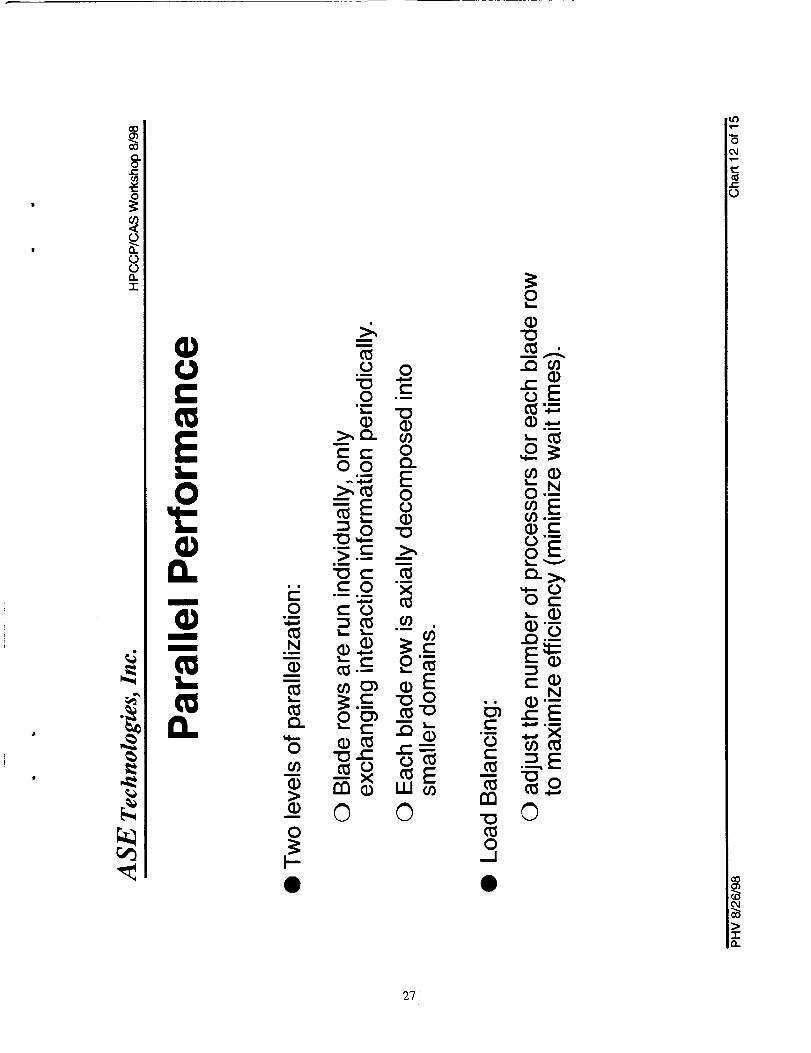
system of the GE90 turbofan engine. The code has two levels of parallel, and for the 18blade row full turbine simulation has 87.3% parallel efficiency with 121 processors on an
SGI ORIGIN. Grid generation is accomplished with the multistage Average Passage
Grid Generator, APG. Results for each component are shown which compare favorably
with test data.
Organization
This document is a collection of several presentations, modified presentations (to
eliminate GE proprietary information) and papers which have been written or presented
in support of this task order. They are arranged in the appendices which follow. They
are:
lip
• Appendix A: Parallel 3D Multi-Stage Simulation of a Turbofan Engine,
presented at the 1998 NASA HPCCP/CAS workshop, August 25-27,
1998 at the NASA Ames Research Center.
• Appendix B: Application of Multi-Stage Viscous Flow CFD Methods for
Advanced Gas Turbine Engine Design and Development, also presented
at the 1998 NASA HPCCP/CAS workshop, August 25-27, 1998 at the
NASA Ames Research Center.
• Appendix C: GE90 Simulation which has been slightly modified from
the presentation given at NASA Lewis Research Center on October 16,
1998.
• Appendix D: "Multistage Simulations of the GE90 Turbine" paper which
will be presented at the 1999 ASME IGTI conference.
• Appendix E: Excerpts from the 1999 IGTI scholar lecture paper by John
J. Adamczyk "Aerodynamic Analysis of Multistage Turbomachinery
Flows in Support of Aerodynamic Design."
• Appendix F: Combustor Analysis description for the efforts to model the
combustor in APNASA with source terms. This approach was later
replaced by a simple boundary condition treatment for representing
combustor profiles.

All slide, chart, page or figure numbers will be referred to using the following
format: (Slide 1, A), where the slide number is referenced followed by the appendix
letter.
Overview
An overview of this task order is shown in Appendix A. On the title slide (Slide
1, A) is a picture of the GE90 compressor. Each blade row is shown with the contour
representing a quantity calculated when running the full compressor with APNASA.
(Slide 2, A) shows how a building block approach has been used in this project.
First, rig simulations have been run including the low pressure turbine (LPT), high
pressure turbine (HPT), high pressure compressor (HPC) and a GE90 booster rig. The
PIP (Performance Improvement Program) HPC is a new 3D Aero compressor which has
been designed to have greater efficiency than the original production compressor. In
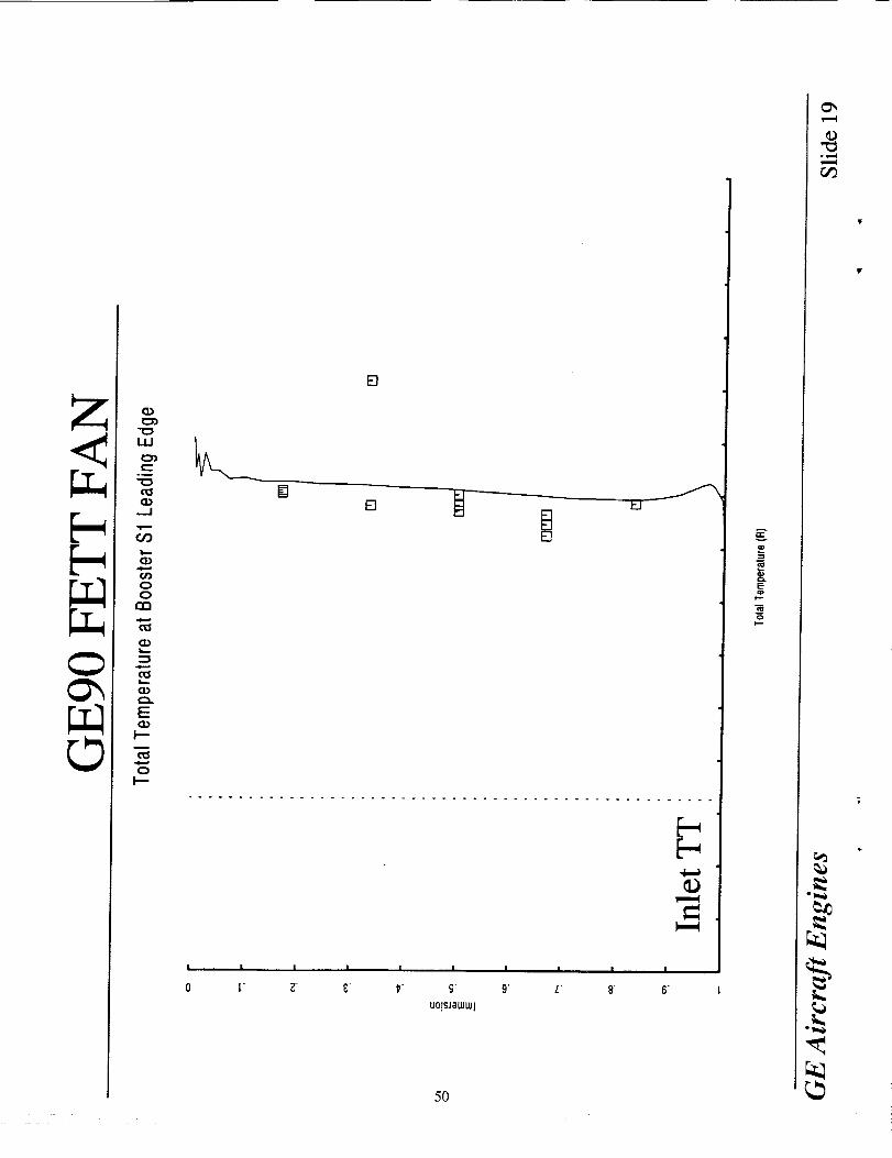
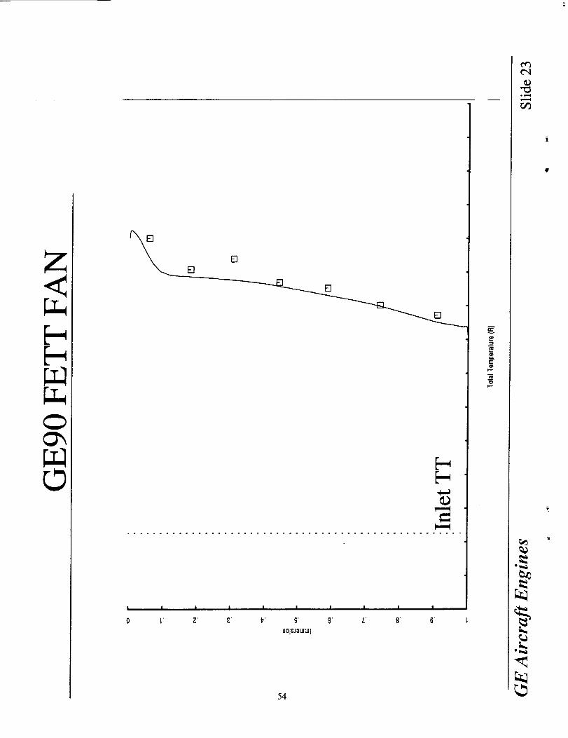
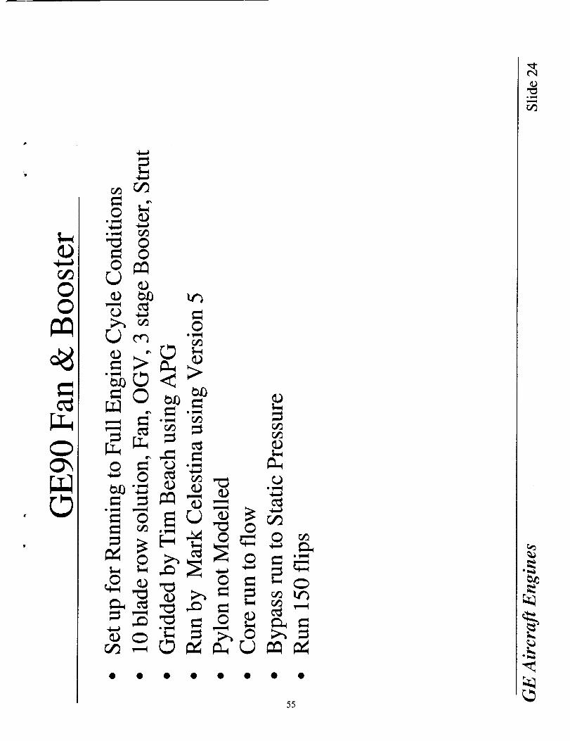
addition to the these rigs, a fan simulation has been run consisting of the fan, fan OGV
and booster stator 1. Only in a turbofan engine can a fan of this size be tested. The fan,
booster and bypass were then put together and run as a component.
Two systems are then put together at the takeoff Mach 0.25 cycle condition which
has been chosen for this simulation. These are the full compression system and the full
turbine system. These together then comprise all the turbomachinery of the GE90 engine.
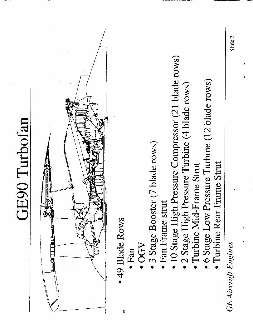
(Slide 3, A) shows all 49 blade rows of the GE90 not including the pylon. All
these blade rows have been modeled as part of this project.
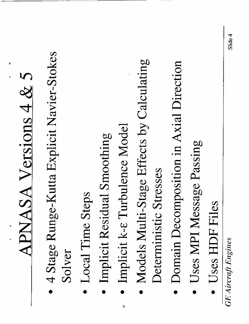
The foundation of this effort is the CFD code APNASA. On (Slide 4, A) is a
description of the features of the latest versions of APNASA which have been developed
at GE. Version 5 has radial multi-block capability. Both Version 4 and 5 allow for non-
pure H-grids in dealing with the multistage closure, although pure H-grids can still be
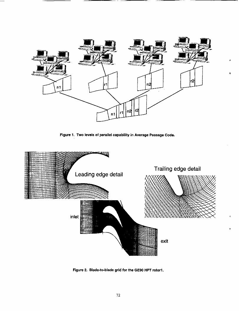
run. Both versions have two levels of parallel capability as shown schematically in (Slide
5, A). Each blade row of a component can be run in parallel. In addition, each blade
can be decomposed into a number of axial sub-domains. Each sub-domain of each blade
row can then be run on a different computer processor in parallel.
The parallel efficiency for this code for an isolated blade row is shown in (SIide 6,
A) for an SGI Origin 2000 as well as a network of Hewlett Packard (HP) workstations.
MPI is used for the message passing. On the SGI Origin 2000, the parallel speedup is
actually super-linear with 2 or 4 processors. This is probably due to an improved cache
memory utilization. Different approaches have been taken in modifying the algorithms in
APNASA to reduce the amount of network traffic. Using a reduced ADI scheme greatly
improves the parallel performance on the network of HP workstations. With this
approach, parallel convergence is not identical to serial convergence, but the converged
solutions are the same. Excellent parallel efficiencies are obtained with this code.
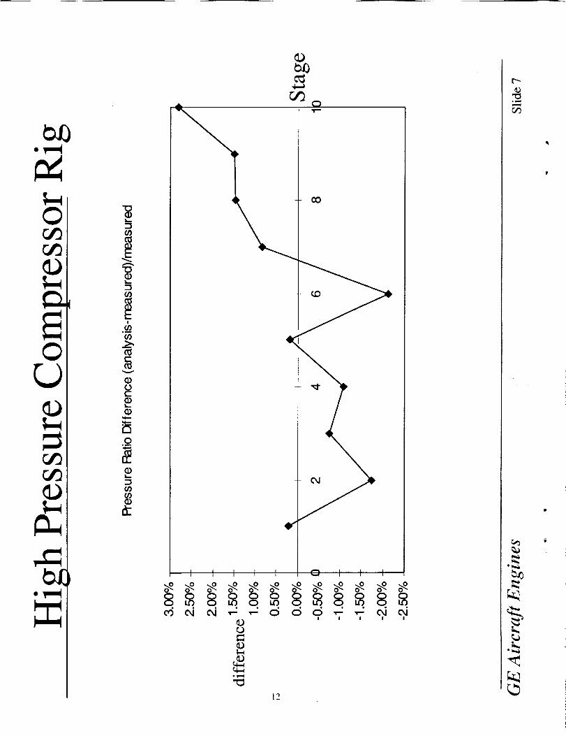
An example 0fthe fidelity of the calculations is shown in (Slide 7, A) which is the
pressure ratio difference between the compressor rig simulation and the measured
pressure ratio for the GE90 10 stage HPC. For each stage, the simulation is within 3% of
the measured pressure ratio.

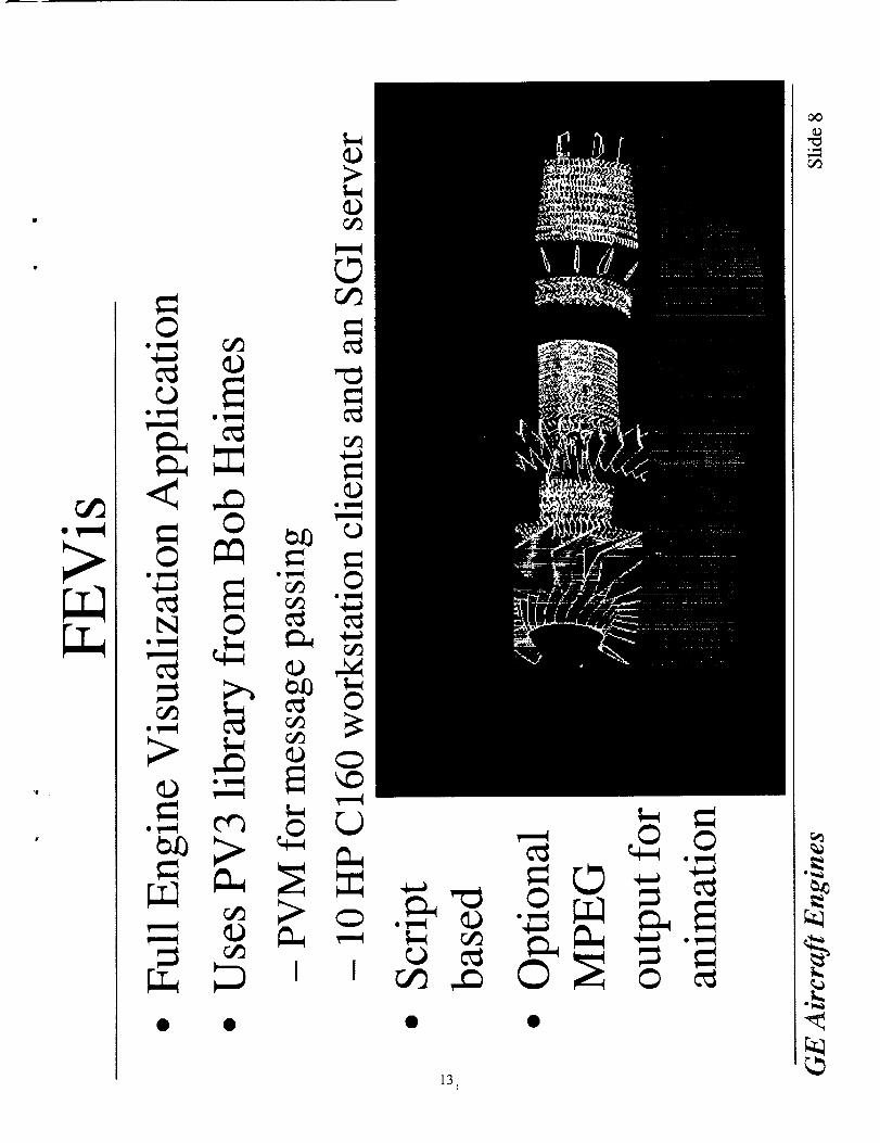
In additionto thecomplexsimulationcapability,ananimationcapabilityFEVishasalsobeendevelopedunderthis taskorder. FEVis canbeusedto simulatetheentirefull enginesolutionwithall thebladerowsatonce. Thecapabilityis shownin (Slide8,A). It is aparallelvisualizationpackageutilizing thePV3library from BobHaimesatMIT. It allowsfor MPEGoutput,which is availablefor theenginesimulation.
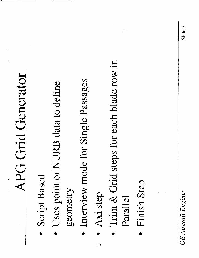
Grid Generation
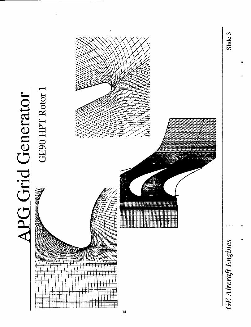
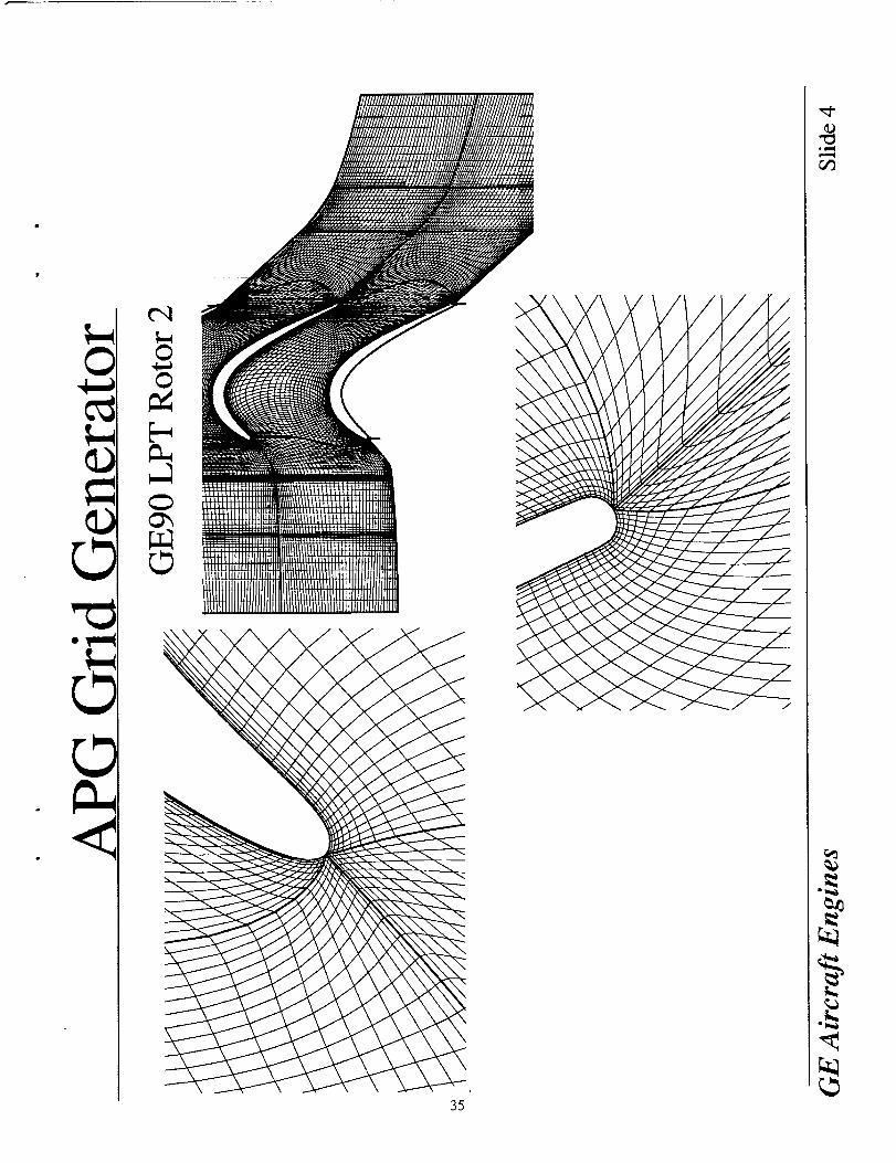
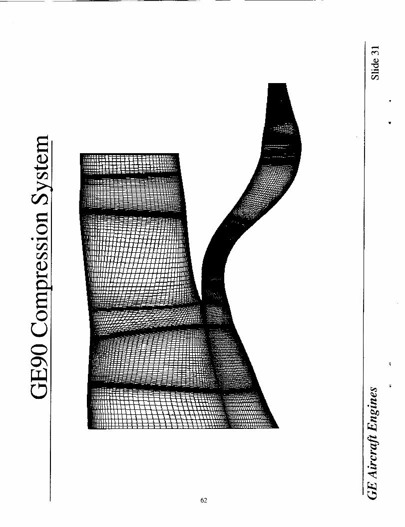
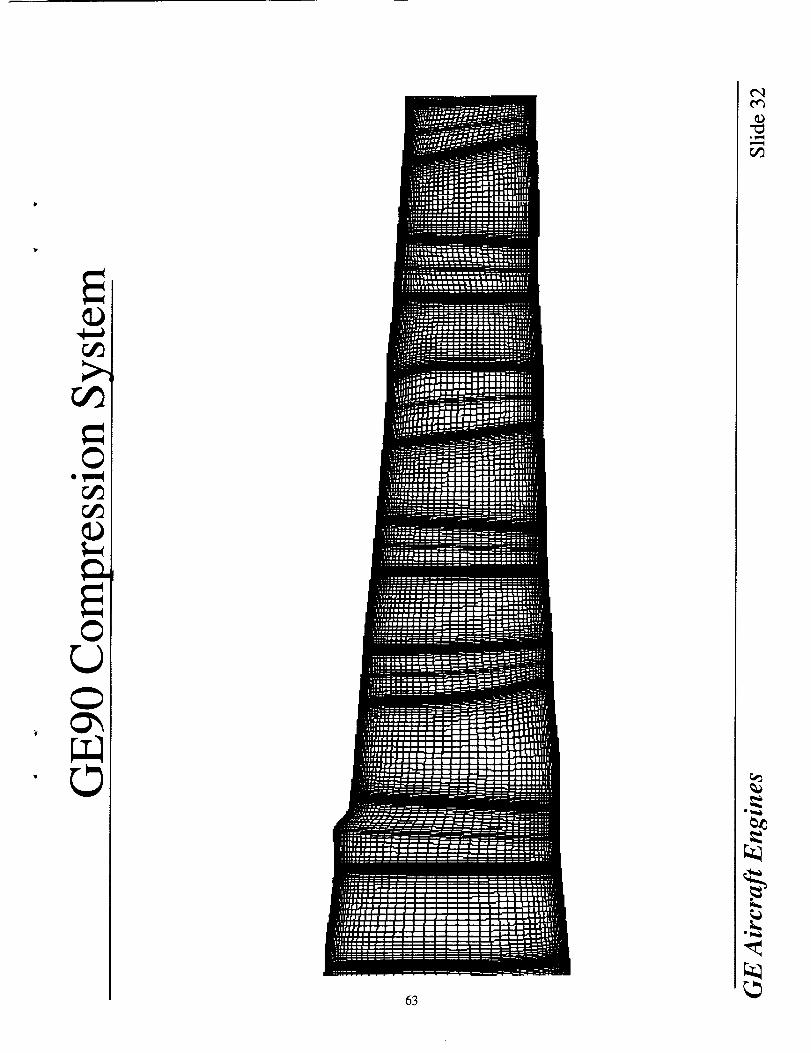
Thegrid generationfor thiswork isAPG. A descriptionis shownon (Slide2, C).Examplesof non-pureH-gridsfor turbinesareshownin (Slides3-4,C). Theaxisymmetricgridsfor thefull compressionsystemareshownin (Slides30-32,C). Forthecompressionsystemsimulations,apureH-grid is usedwhereasfor theturbinesimulations,anon-pureH-grid isused.
Compression System
Thecompressionsystemis describedin (Slides5-32,C). TheHPCsimulationisdescribedin Appendix E under the subheading High Speed Ten Stage Compressor
(pages 15-16, E) and (Figs. 14-22, E).
Combustor
Appendix F describes the Combustor Analysis strategy which was initially
adopted for this project. Due to time and funding constraints, this approach was stopped
in favor of a simple boundary condition specification approach. This current procedure is
also more consistent for future coupling with a combustor code.
Turbine System
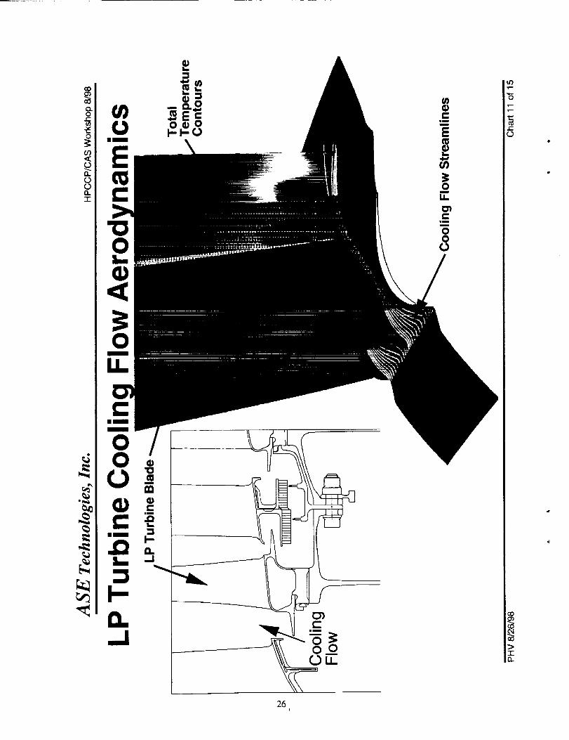
Appendices B and D are detailed descriptions of the Turbine System simulation.
In addition, (Pages 17-18, E) and (Fig. 25, E) also mention this turbine system
simulation.
Parallel Efficiency
The parallel capability of the APNASA code has already been briefly described in
the overview section above. In addition to this description in (Slides 4-6, A), there are
(Charts 12-14, B), (Page 6, D), (Fig. 1, D) and (Figs. 15-16, D) which describe the
parallel performance of APNASA in more detail.

In additionto theparallelcapabilityof the solver APNASA, APG and FEVis,
both of which are described above, are designed to run in parallel. APG can grid each
blade row separately once the axisymmetric grid has been created. And FEVis uses PVM
to collect information from client processors for the full engine visualization.
Applications in Design
The excerpts from the 1999 ASME IGTI scholar paper describes how APNASA
can be used in design. The HPC which has been analyzed under this project is presented
in this scholar paper to demonstrate how this method compares with other design
approaches and experimental data. The GE90 HPT, which is also part of this work (in
addition to the NASA AST work being done at GE under AOI 5), is also mentioned in
this paper.
Conclusions
The components of the GE90 turbofan engine have been analyzed using the
multistage CFD code, APNASA. The components analyzed are the fan, fan OGV and
booster, the 10-stage high-pressure compressor and the entire turbine system. This is the
first time a dual-spool cooled turbine has been analyzed in 3-D using a multi-stage
approach. Grid generation has been accomplished with the multistage Average Passage
Grid Generator, APG. Results for each component are shown which compare favorably
with test data. The successful flow simulation of the fully coupled high pressure and low
pressure turbines has prompted GE to adopt the use of APNASA as a tool to improve
design confidence on future turbine designs. The code has two levels of parallel, and for
the 18 blade row full turbine simulation has 87.3% parallel efficiency with 121 processors
on an SGI ORIGIN 2000. The accuracy and good parallel efficiency of the calculation
now allow this code to be effectively used in a design environment, so that multistage
effects can be accounted for in turbine design, within the short design cycle times
required by industry.
Future Work
The full turbine system has been analyzed as well as each component of the entire
compression system. The full compression system comprising 31 blade rows has been
set up, but still needs to be run to convergence. This will be done under a follow-onNPSS task NAS3-98004 Task Order #9. Also a cycle condition for the new production
GE90 with the 3D Aero compressor will be determined, and this turbofan engine
simulated.

Appendix A
rh
Parallel 3D Multi-Stage Simulation of a Turbofan Engine
presented at the 1998 NASA ItPCCP/CAS workshop, August 25-27, 1998 atthe NASA Ames Research Center
5

©
I
©
61

0
©
0©
!-
__1
0n
n
r_
00
CD _
00
-!.-
_o 0O_•-F -kC C
Y
C0
E
O0
0
0
cO "Ov_
m
C
.0
O0 v
im
0 :_0
Y
CO
Cum
CIllmm
Ii
©
©
0
°_
°_._
o_

©
©
i
lO
olml
CJ9
o_k_

oo
%%%_% 0<_ 0
• _
%%
%%
dnpaeds
%%
%%
o_ ¢) __,;
._ %%%% 0
a/_°%
1
I I I I I I t I I
dnpeads
.___
°_ _ _ __.._'_ N N
o _.
__ _._.__
• 0 r._
E
CO
o
11
°_
o_
i.m
c/)
Cc_
CD0
1,D
Q
0
oo
Lt_ , •
• v.-.(
12
L_
"0
cD
O0
r_
o_

Appendix B
Application of Multi-Stage Viscous Flow CFD Methods
for Advanced Gas Turbine Engine Design and
Development
presented at the 1998 NASA HPCCP/CAS workshop, August 25-27, 1998 atthe NASA Ames Research Center
[5

co
co
c-
o
GO
0
n00O."I-
U_
CL0t-
¢-
¢-
rT_
I
0o
>__L
16
t
co
oo
8
_oi
i¢)
oO
$
n
17

o8o
C0",,_
O0
c_cE
°_ _oE
-8 _• o_ o•
_._' _ _
<,.- ,.- o _ _
o'_ oo _ "_,_.,_ ._o _ ._0"_ 0
o _._•-o _o c°o,.- _._ - 0 0
090 _ W
• • •
0
18

O0
8-
o
19

co
Go
.,9°
o
r_
I
20

m
m
0
0
n
0.._
E__,,-v
M,,,,-
I •
25 _
moc
t- c
.__25
.--. 0
E _
0
0tm
"0
00
c-
O.0
0I
©
-d0
m
000
0
0
or)0
_m
O.1
c
"1-
0rn
©
0m
m
0or)
M,,,,,,
0
or)
00
0
0
0
m
0e-
m
©
)
i021

S_
>
22

1
I*
8
,j
r_
T_T Io
23

(l)
(3
0..T
0
im
Im
m
m
LL
L_
C_
w_
er
24
o
C_
0.T
!--
Em
,idc_
mmm
Em
In
25
o
co_mao
o
O_<
tl
Q."T"
0 8
0
26
u'),rm
t-
0
I:1.
2?

Q..0r-u)-Eo
0')
n
0.-r"
0')
Ilmmm
U
0
"0
Niim
iIm
o
.__ _
_o_.
m
E
n-
"0
m
sJosseooJd Im,O.L%/P!JID Im,O.L% co
2,8:

oo
Q.O
r_
Jol.oe:l dnpeeds lelleUed
'r'-"
'5
T--
5
i291

o
D..00a,."1"
a,_
"_ ._0 >0.___..C:O')O
¢,/)__ ...c::
,.__)
"_0_{.._o _ -,-.'
_>,,_.,_,.,-.,_"_ {"- .m
tj_ o .,..,,
C:Z._
0
0im
i
mw
ua
.=_
a_g 8
im
m
0
E0
00
_"0_
i
_>
0.- o_>,,_
,,,_- ,.,{_
_-_0
omt.-
_o
• • •
I
3O
Appendix C
GE90 Simulation
slightly modified from the presentation given at NASA Lewis Research
Center on October 16, 1998
31

©
o_-_
O_
\
32
"0
olm_
°lm_j
_q
©1
<
33
o_
a
o_
©i ©
©
m
] I L l L
| i 1 l .
i_2 c :
34
©
• ,p-,,4
35

0
0
36
t_
._

©
m
I1.
F-a.[
aJnssaJd IB_oJ.
C_T-
n-
2ff
® &
o.
C_
O
37i
aJntRJoduJa.L Im,OJ.
Q
o3
(D
0

o_-_
©
©
o_,_
©oT--_
c_
o_
©
op,e_l ejnsseJd u! JOJJ=1%
38
©
I
°_Jl
c_
c_
©
t'--
o_

©
©
o_
"0
©
©o_,m4
0_0
l
I I I f I I I I
0 0 0 0 0 0 Ob Ob
o!J,eEI e_nssaJd e6e_s eA!_elaEI
p,.o_O
39
O
cO
r£3
O
._=,_
C_
C_©
O
©
O
d_
o
d_
©
=
©
0
cO00
I " I L ] I I 'I'"
,- ,,- ,- d d d
o!|eEI aJnssaJd a6e|s a^!J,elau
0
cO
c_J
d
C_
0
40

o_
©r.#'3r..#3¢i
©
¢)
r._r.43<1.)
• l,,,-i
1411ttl
<'" Ij#j_.F
0 V _' C' I," 0" 9' L" 8' 6"
t_lNI
[]
,.q.
0 L" _" C' _' 8' 9' L" 8' 6'
PIll
4<,%
!=::l..
co
<_
4<%
41
i
._ BM __:1 rq [] E] l=
/, (_ /I i / {
• %
t \. I ,/ ":.
P,
\1
II
I/llNI
J
i.,---..,_ j
./i!m/ \
i
i_#
i
/
i_' C' l," G' 9' L" 8' 6"
14141
,,,...
i-.-
A [] E 1_.,/E /
J
l _' 0' _" S" 9" L" 9" 6'
" II
iR
o_
c#'J
r_

©
©
-v--_
e.o
JEl
/\/ _\_I_ t
i......... j
I. _ _" tr c_" g- L" 8' 6'
/
I,,..
F-]
/
/
//
/
[]
OJ L" _" £" Y _" 9" L" S' 6"
N
J
//
/
\
J
/
L" "_" _" Y _" 9" L" 8" 6
V_ifll
II
\[\i1I!
42
"_ ..____..__ _ --_
r/E E = '-
t" _" _:' t" _' 9' L' g' 6' i
I_1_1
/f\ ,,
L" _" £' t_" S' 9' L" 8 6'
PI_]
I:Z
e.-,
w.=d
¢)"c3• w="_
r./3
r,¢
e_

I I :
V _" _" _" g" 9" Z" 8" 6"
lflV_l
q
rl
3Jl
IJ
L" _" _ _" S" 9 L" 9" 6"
_V_I
== -- 'M _ _.--_-_
0 L" _" _" _" 8" 9" L" 9' 6"
F1ii []
/ii []
\,-,\
zz". ;
I
---I
',\
tI
I
/
[]
1
i
/
43
("4v--,.,I
©i _,,-I
o_
_c
r_k_

©_f3
©
rJ_
]
\ []
_ \
\\
°lI °
i
://
/! • ,, /
E_I! /
j%.
I
.w
w
I_INI
i\\ r"l
\\
\ J
//
0 [" _" C' I,' _' 9' L g 6
\j_
_ ..___...J
/
/!
_' g' ¢' t,' _" 9' L' 8' 6"
0 |" _" 8" f'" _" 9" L" 8' 6' i
\ /
0 |" _" _" t" ¢_' 9' L" 9" 6' [
44
...,.
° 1===1
r../3

©
d.)0%
L" _" C' _" _" 9" L" 8" 6' I
-.-----.._.._ _
\\
0 !." _" C' t," _' 9' L" g' 6' J.
INIql
.-...,..
0 |" _* C' t_" S' 9" L 8' 6' |
E7
EI
0 | _' _' t," _' 9' L" 9' 6' i
II
J
0 t" _" _' t,' _ 9' L* 8' 6' |
_1
\
|" _' _' t," 8" 9' L" 9" 6" i
Ittlttl
45
rd3

©
r./'j
lJ
if0 !.' _" C' t,' _' 9 t" 8' 6' i
0 |" _" _" _" _" 9" L" 8" 6'
0 I.' _' C' t,' _' 9' L" 8' 6' t
0 L" _" C" t" _" 9" L fl" 6
INI_I
0 r _' _' l,' ¢_" 9" L" 9" 6 I.
_ittl
-.-......__ -----,---- _ ,\
l." _" C t_' _' 9' L' 8' 6 !.
IttlNl
46
_th

a,
•..-._.._ __._.,..l_____4.,_.-_ /of)
0 !. _' _' IT' _' 9" L" 8 6' t
i'tifll
f_
0 _ "_" C" 't r;" 9" L" 8 6" I
_V_I
•j /f_
0 _" _" C" tP" _" 9' L" 8" 6" |
47
r_ ._m
\%
0 [" ?," P," _" ¢J" 9" L" 9" 6" i
IN_I
\
0 _" "_" g" t" _" 9" L" 8" 6" i
_1
_D
r./3
r_
*_
o_=,_
©C/3
©
©
_P3
\
\\ /
j
0 _" _ I;' t, _;' 9' L 8' 6"
_1
J
\
\ jJ \
0 _" _' I;" I_' g' 9' L' 9" 6' 1
INPtl
_ _ _.._..I _r _
Iql'll
0 L" i_' I_" '_" _' g' L" g' 6 I_
I]
]
0 t' _' E:" tl" _;' 9' L" 8" 6'
48
£)
,w,=l
r./3
°_

,,=,
.__I
0
=c_
Ci_
©
I I I I i
0 L" _' _' _
I
g.
u0!s_wtul
49
G)
O-f
w
O0
[]
[]
©
_ E;' _" G 9"
uo!sJawWl
L" 6"
5O
I,,--
C/]
e_

Z<
_q
I I I I I
0 L" _' £' I_'
I
S'
uo!sJe_uJi
I
9'
!
8"
I
6"
5]
c_
C_
ovml
r_
r_

[]
B [][] E_[]
[-
I I I I I I I I I
0 L' _" _' t,' _' g' C 8"
UOISJeUJLUI
52
A
v
¢12
o
t'q©
o_
c_

Z.<
0
[]
©
! ! !
u0!sJeWWl
53
Q=
o
r._
r_
r_
o_
r_
0
E][]
I I .... I I I I I I I I
0 L _" £" t'" c_' 9' L' 8' 6'
u0!sJeLUml
54
I,.--
w
o
c/]
¢)
©©
0
r...q
"_ 0
rj_ lt_
r..T..] ., _.,.
,,-, © "_,._ ,..._ ¢_ "-'_
• ,-_ _ _:_
55
o_

©0
0
%_ E
,kt_____. F ""F
f ''-'-" 11 j f _ 0
i0 t g" C" 1," 9" 9' L" 8' 6' |
0
¢:-,
0 L _ _ t_" _ 9 L 8 6*
I_I_1
°o
. - 1_-I . .
r./3
©
0 L g C t _ 9' L 8 6' |
Z
©• _,-=i
©O
] o ° . °L..
[] " -
f \
L" _" C' t,' ¢J' 9" L" 8' 6" |
_l/'tl
.=.E '"
_. __._-. __
L' _' _' t_' _' 9' /-' 8' 6" 1 f," _' C' I,' S' 9" L" 8' 6" I.
_1 ININI
56
©
o_-,_
0_G

©r./3©©
O
. rO
"el
\\
-E'
\
• j r
L_
f _'" O
. r't-,-.
0 r _ I:' t_ _ 9' L' 9' 6' 1
t_lfll
._]" • "E I I IB I_ I t I" "
0 r _ I_ t, S 9 L" 8' 6' I
#_1
-El-- -E -- [] --- E .... E
r _ c tr S' 9' L' 9' 6' |
_1
4
=©
.,=°_
=
111 ff *1
|' _' _ 1_' _' 9' L' 8' 6' 1
c_©Zc/)=0
-,_
o __o__< ---% ._-" .El-. El--; -FI'" C _ ¢)
=
©
=
0 r g C t, S 9' L' I1' 6' L
_1_1
0
-E]-- E" El O
r_0 r i_ I;' t" _" 9' L" 8' 6" 1
<
5"7
-8o_1
c/)

©,4...a
©©
0
u'>
///
t" _' C' t,' _;' 9' L" 8' 6" I
PiVtl
\
I." _' C' t," _;' 9' L" 6' 6' I
PJ_I
........-_------ _/.1
/[/
0 t' _' C" t,' _' 9' L" 9 6 I
\
O3
0 !." _' _" t," ¢_' 9' L' 9" 6" I
f-
0 |" Z" C" 1_' _' 9' L" 8" 6' [
.,,..:
|" _' C' _' G" 9' L" 8' 6" I
I_INI
58
• _,,,,-,I
=._
>
0
GO
.,iml-¢I
>c,D0
¢)
¢)GO
= I=
o_1
("4
wv

g
59
_0t'_
._

©°_
©
0
©
©
°_,_
60
o_

©
0.v,,_
¢,13
©
0
61
©
*m,q
e_
©
r.,t3
0• ,!,,_
_D
0
62
r._
r_
0° _,,,,_
r.__D
©
63
_q
©,._
r_
" l_'j
.,_

Appendix D
"Multistage Simulations of the GE90 Turbine"
to be presented at the 1999 ASME IGTI conference
65
MULTISTAGE SIMULATIONS OF THE GE90 TURBINE
Mark G. Turner
GE Aircraft Engines
Cincinnati, OH
Paul H. Vitt
ASE TechnologiesCincinna_, OH
David A. Topp, Sohrab Saeidi, Scott D. Hunter, Lyle D. DaileyGE Aircraft Engines
Cincinnati, OH
Timothy A. Beach
Dynacs Engineering Co.Cleveland, OH
ABSTRACT
The average passage approach has been used to analyze threemultistage configuralSoas of the GEg0 turbine. These are a highpressure turbine fig, a low pressure turbine fig and a full turbineconfiguration compris=g 18 blade rows of the GE90 engine at takeoffconditions. Cooling £ows in the high pressure turbine have beensimulated using source :erms. This is the first time a dual-spool cooledturbine has been anal.vz_ in 3D using a multistage approach. There isgood agreement be__n the simulations and experimental results.Multistage and component interaction effects are also presented. Theparallel efficiency of ",he code is excellent at 87.3% using 121processors on an SGI Origin for the 18 blade row configuration. Theaccuracy and efficiency of the calculation now allow it to beeffectively used in a d__'ign environment so that multistage effects canbe accounted for in tuf:ine design.
INTRODUCTION
The high pressure turbine (HPT) of a modem turbofan enginemust operate in an ex"zeme environment of high temperature, highstress, and high speed As such, it must be film cooled and designedfor long life and high efficiency. The heat transfer design requires adetailed knowledge of :he gas side temperatures. The low pressureturbine (Lgr) is desigz_l for very high efficiency and must be able tooperate effectively be_nd the HPT. The requirements for both the
HPT and LPT necessitate a detailed aerodynamic solution capabilitywhich accounts for the film cooling, multistage effects and variablegas properties.
The Average Passage Approach developed by Adamczyk (1986)has been generalized for improved grids by Kirtlo'. Turner and Saeidi(1999) and applied to the complete turbine for the GE90 turbofanengine. In preparation for doing the full turbine, the HPT and LPT rigconfigurations were first validated. These rigs v,'ere designed andtested as part of the GE90 development program. A three quarterscale rig of the 2 stage GE90 HPT was designed and built by GE andtested at the NASA Lewis Research Center. A half scale rig of the 6 "stage GE90 LPT was designed and built by GE and Fiat and tested atGE. These rig tests produced detailed measurements of hub andcasing static pressures and inlet and exit profiles of total pressure, total "temperature and flow angles. The engine turbine simulation was setup based upon a cycle analysis of the GE90 engine at takeoff. TheHPT rig simulation comprised 4 blade rows; the LPT rig was 14 bladerows including the mid frame strut and OGV, and the full turbinesimulation comprised all 18 blade rows.
The present work was undertaken for three reasons:1. To support a full engine simulation of the GE90 in order to
demonstrate the capability of high fidelity 3D ana].vsis for a completeturbofan application. This would allow an analysis of the primaryflowpath when coupled with the full compression system and a model
66

of the combustor,. This represents the first time a _-al-spool cooled
turbine has been analyzed using a 3D multistage solver.
2. To determine the differences between a turbine running at
warm air rig conditions and that running in an engine. For the HPT,
this involves a severe inlet temperature prof:ie at elevated
temperatures. For the LPT, this involves the in_'raction with the
upstream HPT which produces profiles of temperature, pressure and
flow angles. The amount of cavity purge flogs in an engine
application were also much geater than in the LPT rig, which greatly
modifies the hub aerodynamics in the LPT.
3. To validate the method for application in turbine design by
simulating real turbine hardware.
This paper describes the features of the code, APNASA,
including film cooling and the variable gas model used. It also
presents the method of simulating leakage flows due to purge cavity
flows, nozzle under shroud leakages and rotor over shroud leakages.
Following this, the HPT rig, the LPT rig and the full engine
confimlrations will be described. Results for these simulations will
then be presented with particular emphasis on multistage effects and
differences between rig and engine simulations. Following the results
is a description of the parallel capability, of the solver when applied to
the 18 blade row full turbine configuration.
METHODOLOGY
Three methods have been used by researchers for multistage
analysis. These include the mixing plane approach as described by
Dawes (1990), the average passage approach of Adamczyk (1986),
and the fully unsteady approach similar to Chen. Celestina and
Adamczyk (1994). A full unsteady analysis for a problem of this scale
is still beyond the computing capability currently available. The
mixing plane approach produces an entropy jump at the mixing plane
as demonstrated by Fritsch and Giles (1993). Especially for HPT
turbines with large circumferential variations, this can lead to large
errors. Therefore, the average passage approach has been used to
simulate the multistage environment of the turbine. This has been
shown by Turner (1996) to work weU for an LPT application. The
ability of this approach to capture most of the multistage effects is
presented by Adarnczyk (1999).
Numerical Scheme
The foundation of the Navier-Stokes solver is an explicit 4 stage
Runge-Kutta scheme with local time stepping and implicit residual
smoothing to accelerate convergence. Second and fourth difference
smoothing as applied by Jameson (1984) is employed for stability and
shock capturing. A k-e turbulence model is solved using an implicit
upwind approach similar to that presented by Turner and Jennions
(1992) and Shabbir et. al. (1997). Wall functions are employed to
model the turbulent shear stress adjacent to the wall githout the need
to resolve the entire boundary layer.
The solver has been parallelized using MPI tMessage Passing
Interface) to share information across domain boundaries. Domain
decomposition is accomplished "on the fly" by subdividing the grid in
the axial direction into an arbitrary number of domains specified in the
argument list. The number of parallel bugs has been reduced or totally
eliminated by strict adherence to keep the parallel code equal to serial
All blade rows are run for 50-100 Runge-Kutta iterations, at
which time the body forces and deterministic stresses are calculated
and written to a file. This is one outer iteration, or flip. At this time.
the files are distributed to the other blade rows to update the
multistage effects.
Averaoe Passao_eAeoroach with Generalized ClosureA more general form of the average passage closure first
developed by Adamczyk (see Adarnczyk, Celestina and Mulac (1986))has been developed by Kirtley, Turner and Saeidi (1999). It allows for
non-pure H grids, as show_ in Fibre 2 for the GE90 HlYl " rotor I.
These grids have been generated using APG, a grid generator specially
designed for the Average Passage Code with the generalized closure
implementation. Compared with the pure H-grids required by the
previous closure implementation, these grids allow much better
leading and trailing edge or_ogonality and resolution which improves
accuracy and the convergence rate. The closure requires overlapping
grids so that the determini_c stresses from one blade row are appliedto other blade rows. This allows blade row interactions such as
spanwise mixing of temperam_, wake blockage and potential field
blockage due to blunt leading edges to be modeled.
The desired near wall fcid spacing can be characterized by the
dimensionless quantity y" which should be approximately 30 when
wall functions are used. Grid geaeration was carried out with this goal
in mind, while also balancing the need for good leading and trailing
edge resolution. The actual y" values on the pressure surface of
Nozzle I were approximately 20. Tip gaps over the unshrouded HITI"
rotors have been modeled with 4 cells. Periodicity is applied across a
void representing an extrusion of the blade to the casing. Overall grid
resolution has been set based on a detailed grid study of the LPT
nozzle 1 as an isolated blade row. Grids were chosen which produced
accurate flowrate and loss calculations. This gridding approach was
then applied for all blade rows. The resulting grids had 50 spanwise
grid points. The number of blade-to-blade grid points varied with
blade row solidity; 41 blade-to-blade grid points is a representative
number. A minimum of 72 points from leading to trailing edge were
used. The number of grid points in the axial direction varied
depending on the chord and axial gaps of each individual airfoil.
As mentioned, the average passage approach uses overlappinggrids. When validating the liP turbine, it was noticed that the extent
of that overlap should only be half way through the downstream blade
row. If the overlap extends further, the upstream blade row wake
produces an entropy decrease _ich is not plausible and does not
compare favorably with the measurements. This is due to the closure
not mimicking the true unsteady wake chopping effect. The dominant
effect of the downstream blade row is captured by including the front
half of the airfoil. This effect is the metal blockage of the downstream
airfoil and the bending of the wake streamlines due to the turning of
the downstream blade row. The blockage effect of the upstream wake
through the first half of the blade row is also still captured. Research
is currently underway to correctly model the physics without
truncating the grids, but the mmcated grid approach can still provide a
quality solution if the solution is interrogated correctly. The LPT rig
simulation did not suffer from this problem so overlaps of one blade
row were used. For the I-IPT rig and full turbine, a half blade row
overlap was used for each blade row.
_within numerical precision). The overall solver has two levels of
parallel capability as shown in Figure 1. The first level is to solve Model for Real Gas
each blade row in a multistage component. The next level is to solve A model for real gas effects which treats _/(the ratio of specific
each blade row on several processors, heats) as a linear function of temperature was presented by Turner
67
(1996).In that implementation. 7 was treated as an axisymmetric
quantity. With the new closure implementation, this has been
generalized so T is now a thr_-dimensional quantity. This is very
important for a turbine where the inlet total temperature can vary by
1000 degrees Rankine, and large variations in temperature can occur
circurnferentially due to wakes and secondary flows. Figure 3 shows
how well the linear model compares with the actual real gas for 7, Cp
(the specific heat at constant pressure) and H (the enthalpy) for a range
of temperatures typical in an HPT at takeoff conditions. These
quantities are also shown assuming a perfect gas at constant 7,
resulting in a large enthalpy shift. With cooling flows modeled as
sources of mass, momentum and energy, this allows the cooling flow
to enter at the correct enthalp', level in order to achieve the correct
energy balance.
One other assumption which has been used is that the ideal gas
constant, R, is constant. For a cooled turbine in an engine
environment, there are products of combustion in the flow entering the
first stage turbine nozzle, However, the cooling flow does not have
these products of combustion. This gas property difference leads to a
different R. The energy source term of the cooling flow described
below accounts for this effect, although this leads to erroneous coolant
film temperatures and other errors. A more correct approach is to
track the products of combustion with a species equation and use a
variable R. This has not yet been implemented so an average R for the
turbine has been used.
Source Terms to Represent Cooling FlowA source term approach described by Hunter (1998) is used to
simulate the film cooling on the cooled airfoils, the endwalls and for
some of the gaps with purge cavity flows. Sources of mass.
momentum, energy and the turbulence quantities are specified in each
cell adjacent to a surface with film injection. A row of cooling holes is
actually modeled as a slot because the grid is not fine enough to
capture the effect of each discrete film hole. Several inputs are
required to specify the source terms. These include the coolant mass
flow, the geometric angles of the hole centerline, the hole size, the
coolant supply temperature, an approximate discharge static pressure,
the turbulence intensity and the turbulent length scale of the coolant.
With this information, the mass flux. energy flux, turbulent kinetic
energy flux, turbulent dissipation flux and the total momentum fluxcan be determined. The source term in a cell is then set to the
calculated flux. The unit vector of the momentum flux is specified
tangent to the hole centerline, so the momentum flux in all three
directions can be specified. This approach picks up the macroscopic
effects of film cooling so the overall mass, momentum and energy are
correct with the momentum applied at the correct angle relative to the
blade or endwall surface. Figure 4 shows the contours of absolute
total temperature on the pressure side of HPT nozzle 1 for the engine
configuration. Clearly visible are the rows of cooling holes.
In addition to the source term approach, there is a method to
specify endwall leakage due to shroud leakage and purge flows. This
method is applied as a code input. It differs from the source term
approach in that the axial and radial momentum terms are updated as
the solution converges. The leakage model is more straightforward to
apply. Figure 5 shows how this model is applied to the under-shroud
hub leakage across LPT nozzle 2. The velocity vectors crossing the
endwall show where the leakage model has been applied. Also notice
how the hub flowpath has been specified to model the real nozzle hub
geometry. The effect of leakage is quite pronounced on the endwall
temperature profiles. The amount, temperature and level of swirl for
the leakage is input and held fixed as the solution converges. This
input can be calculated from an assumed pressure drop across an
orifice with a specified flow coefficient. This process has been
automated using a proprietary, labyrinth seal analysis code that requires
the clearance, pressure drop and seal teeth arrangement as inputs.
These leakage flows were then held fixed for the average passage,
analysis.
q
TURBINE SIMULATION CONFIGURATIONS
Figure 6 shows the geometry modeled in this study. For each of
the configurations, total pressure, total temperature, the radial flow
angle and zero swirl were specified at the inlet. At the exit, the static
pressure was specified. For both rig configurations, the design intent
geometry was used.
The goal of the rig measurements, the data reduction, and the
choice of instrumentation used for these rigs has been to obtain turbine
performance. The use of these data for validation of CTD simulations
is only a byproduct of this primary goal. The biggest impact is that the
energy output of a turbine is measured through a torque measurement
of the shaft. Torque times wheel speed gives the power. The
temperature measurements are taken to obtain radial variations in
temperature and not the absolute level. The variation is obtained
accurately without detailed calibration of the thermecouples. This
detailed calibration is therefore not done. Static pressure
measurements are taken under nozzle platform overlaps in the hub of a
turbine. Due to detailed cavity aerodynamics, this is not the flowpath
static pressure. In addition, upstream turbulence has not been
measured. Upstream turbulence intensity values of 5% have been
applied for the HPT and LPT rigs, and 10% for the full engine.
Hi_ah Pressure Turbine RioThe _ rig geometry is shown in Figure 6. It is a 3A scale
cooled rig of the actual GEgO HPT which was designed and built atGE Aircraft Engines and has been tested at a NASA Lewis Research
Center test cell. The actual configuration also included the strut and
first LPT nozzle. Only the first four blade rows have been analyzed
here. A simulation was set up to match the rig test conditions.
Low Pressure Turbine RioThe LPT rig geometry, shown in Figure 6, is a ½ scale rig which
was designed and built by GE and Fiat, and testedat GE. It is a six _
stage high efficiency LPT. As shown, the turbine center frame and
turbine rear frame struts were tested and included in the analysis. Thisqlv
simulation was set up to match the rig test conditions at the LPT
design point.
Full Engine Turbine ConfigurationThe full turbine configuration is shown in Figure 6 at full scale as
it exists in the engine. A few changes relative to the rig designs had to
be implemented for the production engine. The most notable is that
the first stage nozzle throats had to be opened up to alloy, more flow
in the growth production design. Overall boundary conditions and
levels of cooling flow were set up using a cycle model of the GE90 at
sea level takeoff, and at 0.25 Mach number. This cycle model has
68

l
empiricism derived from rig and engine data and represents a good
macroscopic view of the engine. The temperature profile at the inlet to
the turbine is based on analysis and testing of the GE90 dual annular
combustor at takeoff. Detailed distribution of cooling flow is based on
analysis models of the serpentine passage cooling circuits. To match
the cycle flow, the HPT nozzle throat area was increased 1.7cA relative
to design intent. This was accomplished by re-staggering the nozzle
0.35 degrees more open. This is a very small angle difference and was
rationalized that area measurement error and assembly tolerance which
is estimated at approximately 2% is greater than this change. Correct
work splits among the stages and the future mating with the rest of the
turbofan engine analysis requires that the mass flow be consistent with
the cycle. This was accomplished by adjusting the throat area in a
reasonable way.
RESULTS
Each simulation has been run until the axial variation in flowrate
accounting for cooling and leakage flows became less than 0.2%.
Other parameters were also monitored to verify that the losses and
work were not varying. Use of mass flow as an overall _ide is
appropriate for this subsonic turbine application. Because the
multistage matching changes the mass flow, the mass flow for this
application only settles out after other quantities have settled out. For
each simulation, small changes in the simulation parameters have been
made as the solution evolved. These included the nozzle re-stagger
described above and a modification of coolant supply temperatures for
the cooled turbine based on a re-evaluation of the assumptions. Noneof these cases was started from scratch and run to convergence without
a simulation parameter change. The full turbine simulation took about
20,000 Runge-Kutta iterations with 50 iterations per flip or outeriteration. If the full turbine simulation was started from scratch with
no changes in simulation parameters, it is expected that convergence
could be achieved in about 10,000 iterations. The rig simulations take
less time because of the reduced axial extent over which pressure andvortical waves need to travel.
Table I is a comparison of the rig analyses with experiment for
one-dimensional overall quantities. The results compare well except
that the flow is high in the HPT and low in the LPT relative to the
experiment. It is not known why the HPT flow is high. but as
mentioned above, a very small change in flow angle makes a bigdifference in flow. There can also be differences in actual throats
relative to what was analyzed due to measurement and manufacturing
tolerances. Coolant injection angles, especially at the trailing edge
slots, also strongly affect the flowrate, but may not be modeled
accurately. The LPT throats are not as difficult to measure as in the
HPT since the exit angle is not as large. Therefore the geometry is
probably not the cause of the discrepancy in the LPT. More likely, it
may be due to the assumption in the turbulence model that the flow is
fully turbulent, whereas in the rig there may be a large amount oflaminar flow which would reduce the wakes and increase the flow.
The temperature ratios do not match well, especially for the LPT.
These values are also not consistent with the efficiency prediction
which exhibits better agreement with the rig tests. As explained
above, this is because the temperature measurements are made to
obtain the profile shape, not the level, since the overall tem_rature
levels are not rigorously calibrated in the experiments. A torque
measurement is made to get the overall work from which efficiency isdetermined.
Table I. Comparison of Overall Performance of HPT and
LPT Rig Analyses Relative to Experiment. Efficiency is
analysis minus measured. Other quantities are (analysis -
measured)/measured.
Case Flow Pressure Temperature EfficiencyRatio Ratio
HPT Rig
(4 blade +2.5% +0.4% -1.6% -1.0%
rows)
-2.5 % +0.3 % -3.5 % -0.5 %
LPT Rig
(14 blade
rows)
Profiles of total pressure (PT), total temperature ('IT) and angle
are shown in Figures %9. Rig and engine analyses are compared with
experimental data. At station 41, the PT and TT are normalized by the
average PT and "I7"at station 4 (the inlet). At all other stations, PT
and TT are normalized by the average plane 42 PT and TI" values of
the experiment or the cycle.
In Figure 7, the PT profiles at plane 42 show excellent agreement
between the HPT rig analysis and data. The engine simulation profile
is more hub-strong than the rig, while the LPT rig analysis profile is
flat here since this plane represents the inlet of the LPT rig. At station
48, the strut loss and boundary layer in the LPT rig are well matched.
At station 5, the shape and level match very well.
The TI" profiles in Figure 8 at station 41 show the main
difference between a rig and engine: namely the inlet combustor "17"
profile carries through nozzle 1 t,although mixed) and has large
gradients, especially near the hub relative to a flat inlet profile entering
a rig. At station 42, relative to the experiment, the 'IT profile showsgood agreement except near the hub where the experiment is slightly
cooler than the prediction. The engine was instrumented with
temperature rakes downstream of the HPT, and the full turbine
simulation compares very well to these at station 48. At station 5, the
full turbine comparison has the same overall gradient, but the midspan
temperatures are calculated to be hig.her than the experiment. The
LPT rig comparison of "IT at station 5 shows good agreement. The
overall difference is reflected in the 3.5% temperature ratio difference
shown in Table I, which could be due to measurement calibration
elTor.
The angle profiles are shown in Figure 9. At station 41, the full
engine HPT nozzle l has been opened up to allow more flow and
higher thrust since the rig was built. This is why the flow angle
between full turbine and HI_ rig are different. The swirl differences
are not great between rig and full turbine at station 42. At station 48,
the swirl at the LPT nozzle l leading edge in the full turbine
simulation is different than design intent in the outer 20% span by as
much as l0 degrees. At station 5, the LPT rig and measurement match
well, and full turbine and LPT rig show little difference.
Figures 10 and I I show the HPT and LPT rig static pressure
comparison between analysis and experiment- The overall pressure
drops are very large, so this same information has also been tabulated
in Table II and Table III for the HPT rig and LPT rig respectively.
The pressure taps in the fig are recessed in small gaps in the casing
and mounted under the nozzle platform overlaps in the hub. This is
why the location is described relative to the upstream or downstream
69

nozzle platform in the tables. In general, the comparisons are verygood, The hub pressures compare less welI than the casing pressureswhich is likely due to the location of the pressure taps within thecavities. These cavities are not modeled in the analysis. The inlet
total pressure profile and the exit static pressure profile are specifiedwhich sets the overall total to static pressure ratio of the turbine. Theinter-stage static pressure is therefore a result of the work splits amongthe stages and the reaction of each stage, which is a product of theturbine simulation. The good pressure comparison demonstrates thatboth work splits among the stages and reaction are correctly simulated.
Table II. Comparison of HPT Rig Hub and Casing Static
Pressure. Quantities represent (analysis - measured)/(HPTrig overall total pressure drop).
I-IPT Ri_ Location Casin_
0.63%Stage 1 HPN Downstream Platform
Stage 2 HPN Upstream Platform No Data -1.30%
Stage 2 HPN Downstream Platform 0.30% 0.87%Strut Forward Platform -1.34% -0.91%
Strut LE Rake Plane 0.60% 0.12%
Hub
1.86%
Table III. Comparison of LPT Rig Hub and Casing StaticPressure. Quantities represent (analysis - measured)/(LPT
rig overall total pressure drop).
LPT Ring LocationNozzle 1 Downstream Platform
rr,
Nozzle 2 Upstream PlatformNozzle 3 Downstream Platform
Nozzle 4 Downstream Platform
Nozzle 5 Upstream PlatformNozzle 5 Downstream Platform
Case
Outlet GV Upstream Platform
-0.04%
-1.42%
No Data
0.47%
-0.50%
Hub
0.41%
0.76%
-2.43%
-0.18%
0.37%
-0.60% No Data
Nozzle 6 Upstream Platform -1.39% No DataNozzle 6 Downstream Platform -0.31% -1.43%
-0.24% -0.22°/0
These three configurations represent the three-dimensionalflowfields of 36 blade rows. These are complex flowfields with
variable properties, cooling flows and large secondary flows, There aremany interesting features. One of these is visualized in Figure 12,which shows streamlines that were launched in the purge flow just
upstream of LPT rotor 1. In the engine configuration, the amount ofpurge flow entering here is quite large relative to the fig. Thestreamlines get caught up in the hub vortex and lift off the hub surface.Downstream of the rotor is a contour plot of total temperature showingthat the cold fluid emanated from the purge cavity.
MuttialaC_,/_lmMany axisymmetric solvers used in quasi-3D turbomac_
design systems use a blockage factor or flow coefficient as a soleparameter to accotmt for many effects not described by :heaxisymmetric equations. One of these effects is due to circumfer_:ialvariations within the flowfield. This approach of using blockage has-abasis in matcb.ing measurements given total pressure, :oraltemperature, ang2es, static pressure and overall flow rate. The onlyway to match the flow rate is by introducing a blockage factor which is,less than one. For a given definition of average quantities, such asmass averaged eathalpy, area averaged static pressure, ent_pyaveraged total pressure, mass averaged angular momentum and a_momentum averaged meridional angle, one can determine _is _
blockage factor fi'om post processing any 3D solution. Because of thedefinition, this blockage is due to any circumferential varia_onsincluding wakes, tip clearance flows, secondary flows, leakage flowsand potential effects.
The blockage calculated in this way for the full tu_ineconfiguration is shown in Figure 13. The circumferential variauonsare especially large in the HPT where the temperature varies by overone thousand degrees Rankine due to cooling flow wakes and thesecondary flows which act on the large inlet radial temperaturegradients. In addition, the total pressure and static pressure varytremendously. Values of this blockage factor less than 0.8 exist overlarge re_ons of the HPT. This means over 20% of the flow ar_ is"blocked" in these regions due to these circumferential variations.These effects mast be adequately modeled or the static pres_recomparisons shown in Figures 10 and I 1 and Tables LI and Ill wouldnot be so good. In addition to work splits and reaction, the thrustbalance of the engine can be better simulated. Adarnczyk (1999) hasdescribed flow blockage as being related to the recovery e_gythickness and then related this to the unsteady deterministic flow state.This unsteady deterministic flow state is modeled well using theaverage passage approach and allows these effects to be captured.This is not the case for a mixing plane approach where thecircumferential variations are eliminated across the mixing plane.
Other flow features become apparent in Figure 13 and this type ofplot can demonstrate some overall characteristics of the simulationwith one axisymmea'ic plot. Some of these features are the tipclearance flows downstream of the HPT rotors. The hub leakageeffects can also be seen in the HPT and LPT.
Another multistage effect is that the static pressure downstream ofa nozzle is very different with and without the rotor behind it. "l'h2sisdue to the blade blockage and turning of the downstream rotor and thehigh exit angle of the nozzle. Figure 14a shows the static pressurefield predicted from an isolated blade row solver. The average exitradial static pressure profile has been imposed which comes from a"streamline curvature axisynunetric solver. The boundary condition ofthis code holds this imposed average static pressure while allosingvariations in the circumferential direction. Due to the high exit angie *of the nozzle, the circumferential variations persist far downstream.Figure 14b shows the corresponding plot from an average passage.solution. Notice how the isobars are altered by the close proxirni_ ofthe rotor. The circumferential variations are attenuated by the rotormodeled as body forces. These apply the correct turning, energy dropand blade blockage to simulate the rotor downstream of the nozzle.
7O

PARALLEL COMPUTING CAPABILITY
As mentioned above in the description of the solver, the code has
two levels of parallel capability as shown in Figure 1. Achieving good
parallel performance with this code requires that it be load balanced.
Figure 15 shows hob this has been done with the full turbine 18 blade
row simulation. The size, geometry and aerodynamics of each blade
row is different, and therefore the grid size varied. The load balancing
was accomplished b_ assigning a blade row a fraction of processors
equal to the fraction of grid relative to the total number of grid points.
As shown in Figure 15, this leads to an imperfect load balancing
because the number of processors is integral. The load balance
improved slightly by increasing the number of processors from 60 to
121.
Figure 16 shots the parallel efficiency for APNASA run on an
SGI ORIGIN 2000. The parallel performance of an isolated blade row
calculation up to 8 processors is shown and demonstrates excellent
parallel efficiency. With 2 processors, the speed-up is actually super
linear, possibly due to reduced cache memory misses. The real test ofthe parallel performance is with the real full turbine simulation. The
speedup is plotted against the number of processors assigned to blade
row 2. A case with an equal number of processors per blade row is
also shown and demonstrates the importance of optimal load
balancing. Also shown are the 60 and 121 processor calculations
which used 4 and 8 processors on blade row 2, respectively. The
resulting parallel efficiency is 87.3% using 121 processors which trulydemonstrates the case is well load balanced and the code has excellent
parallel capability.
Currently the code takes 7.3x10 "s see/grid-point/iteration on the
250 MHz SGI OR/GIN 2000 running in parallel with 121 processors.
Since a solution starting from scratch would take approximately
10,000 iterations, a solution of the full turbine which has a total of
nine million grid points would take 1820 processor hours. However,
due to the parallel capability, this solution would be done in 15 hours
of wall clock time utilizing 121 processors. This could be
accomplished ovemi_t, the key criteria for a code to be useful in the
design environment.
The scenario for design use is that a design case can be run
overnight. Automatic post-processing scripts could then be run at the
end of the component simulation. The designer can then evaluate the
design in the morning, make modifications, re-grid the new geometry
and submit a new job to be run overnight. This process would
continue until an optimal design is produced.
SUMMARY
Three GE90 turbine configurations have been analyzed using the
average passage approach. Two of these are rig configurations where
detailed data exists. The third is a full turbine configuration for the
GE90 at a takeoff configuration. This simulation is the first dual-spool
cooled turbine analyzed with a 3D multistage solver. Comparisons
have been made to the measurements, and good agreement has been
demonstrated. Multistage and component interaction effects :have also
been presented which demonstrate why a calculation such as this is
worthwhile. The parallel efficiency of the code is excellent and can
lead to effective use of this code in the design environment.
ACKNOWLEGMENTS
The authors wish to acknowledge support of this work from the
NASA AST program (contract number NAS3-27720, AIO5) and from
the NASA Lewis Research Center N'PSS (Numerical Propulsion
System Simulation) program (contract NAS3-26617 LET#65).
Support by NASA HPCCP (High Performance Computing and
Communications Pro_am) and the CAS (ComputationalAerosciences) Project is also appreciated. Personal thanks go to John
Adamczyk, Joe Veres and John Lytle of the NASA Lewis Research
Center. Thanks also to Larry Timko and Rob Beacock of GE for
guidance on the GE90 turbines.
REFERENCES
Adamczyk, J.J., Mulac, R.A., and Celestina, M.L., 1986, "A Model for
Closing the lnviscid Form of the Average-Passage Equation System,"
Journal of Turbomachinery, Vol. 108, pp. 180-186.
Adamczyk, J.J., 1999, "Aerodynamic Analysis of Multistage
Turbomachinery Flows in Support of Aerodynamic Design," To be
published at the 1999 ASME IGTI Conference.
Chen, J.P., Celestina, M.L. and Adamczyk, J.J., 1994, "'A New
Procedure for Simulating Unsteady Flows Through Turbomachinery
Blade Passages," ASME Paper 94-GT- 151.
Dawes, W.N., 1990. "'Towards Improved Throughflow Capability:
The Use of 3D Viscous Flow Solvers in a Multistage Environment,"
ASME Paper 90-GT-I 8.
Fritsch, G. and Giles, M.B., 1993, "An Asymptotic Analysis of
Mixing Loss," ASME Paper 93-GT-345.
Hunter, S.D., 1998, "'Source Term Modeling of Endwall Cavity Flow
Effects on Gaspath Aerodynamics in an Axial Flow Turbine", Ph.D.
Thesis, University of Cincinnati, Department of Aerospace
Engineering and En_neering Mechanics, November.
Jameson, A. and Baker, T.J., 1984, "Multigrid Solutions of the Euler
Equations for Aircraft Configurations," AIAA Paper 84-0093.
Kirtley, K.R., Turner, M.G. and Saeidi, S., 1999, "'An Average
Passage Closure Model for General Meshes," To be published at the
1999 ASME IGTI Conference.
Shabbir, A., Celestina, M.L., Adamczyk, J.J., and Strazisar, A.J.,
1997, "'The Effect of Hub Leakage Flow on Two High Speed Axial
Flow Compressor Rotors," ASME Paper 97-GT-346, June.
Turner, M.G., 1996, "'Multistage Turbine Simulations with Vortex-
Blade Interaction," Journal of Turbomachiner;,'. Vol. 118. pp. 643-
653.
Turner, M.G., and Jermions, I.K., 1993, "'An Investigation of
Turbulence Modelling in Transonic Fans Including a Novel
Implementation of an Implicit k-e Turbulence Model," ASME J. of
Turbomachinery, Vol. 115. No. 2, April 1993, pp 249-260.
71
._ ........._i___i _.... _
,,,i_ v_"
Figure 1. Two levels of parallel capability in Average Passage Code.
detailTrailing edge detail
inlet
exit
Figure 2. Blade-to-blade grid for the GE90 HPT rotor1.
72

Cpft2/sec2-OR
oo
Y
I
"-2000 2500 3000
eai_tan t y
linearmodel
Temperature °Re_
Enthalpyft21sec 2
constant y
.. _." _ _r_ linear
•_ J_N, model
J real gas
oo W
|l,,,mllml _ ,,llllmm
_000 2500 3000 _20_ 2500 3000
Temperature °R Temperature °R
Figure 3. Linear real gas model used in Average Passage Code at HPT temperatures.
¢
Figure 4. Total temperature contours of pressure side surface of nozzle I showing effect of therows of film cooling holes. Dark - cold, light - hot.
73

Flow VectorsVectors
_ W
t ' i : ....
Geometry_Mod_
Figure 5. Application of leakage model.
Full Turbine Geometry:. 92B On-Wing
High Pressure Turbine Rig Geometry (RV1) - at 133% Scale
J J J
Figure 6. Geometry for full turbine, HPT rig and LPT rig.
74

Station 42 Station 48
01......_;.'--1 o, °_ I sta,o.,0. ;('/ o. _ I ° _
Station 41 .... : 14 / =o., _1 I o.,- _l( - - -_ J I 0.2" I"--% _o.I ,,// |o. _1 I , _1
o._. ,, v. t,i, _. ; o . !:_ °o51 ,// °o5 _l I_ _1,o= ',1 _°'1 .,rl k'l # 1==0151.H=-.: os s . °.B o _i: o... o..t iiEo.;" II Pt/Pt42 PI/Pt42 ON" (_l 'rl
.... ',1 l / ,i........_.J..LQ_.O"
\ 1 _-_'tll]lltl .LU_L_ It Ilfl III \ Solld-FullTurbinet ,.q_ LI_LLLU_ J-LJI II III \ Dash-HPTRig
J I / \_(_- _L.JII \/ Du_-dot-LPTRIg
_ /, _ II-XPRakeData
• - LP Rake DataO - LPTrawme Data
Figure 7. Total pressure profiles in turbine. Each major division is 5%.
Station 42 Station 48
o.i. T._ o.i_ s=_,: ) : i
Sta.on41 =o_ i;'l =.k !--I I °T / o /o .... : !_ : ! o.z io •r_-_, -, 'L: ,',1 _oi III _- . /I
0.1 _ E :" I=, :"
o o_ _ o,o_ !,, ,_ |i x/ ! k i/ I _o,k_l /I
i il i/ :t '°
o._o \ I_tt111t/I Itll III \ ::_,,.,u_\ I_ .W]Ill tlIilLILLIJlII Illl II1 \ _._;:._,.</ I /'_ __ _J.L II tll \ Dash-dotline-LPTRigJ I / _I_ _ l _ • - HP Rake Data
___ t " cJ.-.-,--_r_ / " 0 "LP Traverse Data
_0 _ [ira ¢e) Imd S r_ (ira S]
Figure 8. Total temperature profiles in turbine. The major division at station 41 is 10%. The majordivision for stations 42, 48 and 5 is 5%.
?5

StalJon 42 Station 48
o.i_ o._ ! / Station 5
o= o_ ! oi_ Station41 ¢o_aI_i..,/" I =o.-_ / "I
o._L'J I so._FI[, I so., [i I _o.,L 7; I
-o7 , -,o o ,o 20 -:,-_ o %H,; ,_ o '.
Figure 9. Absolute flow angle profiles in turbine.
5, i .... i
Hub
iiiiiii i,,1111
lID _ub _
Figure 10. HPT Rig static pressure. Line - analysis,circle - data.
Figure 11. LPT Rig static pressure. Line - analysis,circle - data.
76

Figure 12. Streamlines showing purge flow caught in hub vortex. Plane downstream of trailing edge shows totaltemperature contours (dark-cold, light-hot). Full turbine simulation, LPT rotor 1.
i!ii_!Iii!i......Blockage: 0.75 0.80 0.85 0.90 0.95 1.00
Figure 13. Contours of axisymmetric blockage for the full turbine configuration.
77

a.) Isolated Blade RowResults
t
b.) APNASA Resultsj_i_i ]
Figure 14. Static pressure contours for GE90 HPT nozzle I showing multistage effects.
m 10.0 [-
9.o_.".0F I]1_- 70_- oNIIII
°;Illlllllti_ 5.04.0
Bar represents fTactlon of
I] Total Grid60 Processors
I 121 Processors
1111111111111110 15 20
Blade Row Number
fS
14
13
12
S" *
i:6
|D. 4
3
2
1
0
I .... Unear Scalsbl_y ] • "
----B--- S_ Blade Rmv I .."
Ful Turbine, 54pro¢, Net Ba:"nced I •
• Ful TUl'b_e, $Opm¢, Balanced : .* .. t
• Fedl Turldne, 121 ira:c, Balanced i.-'*
' • i r I i t i , l _ r i I5 10 15
Nu_r_ Pro__ Row 2
Figure 15. Load balancing based on grid size. Figure 16. Parallel efficiency.
78

Appendix E
Excerpts from the 1999 IGTI scholar lecture paper by John J. Adamczyk
"Aerodynamic Analysis of Multistage Turbomachinery
Flows in Support of Aerodynamic Design"
79

sor stalls at a flow coefficient near the peak pressure pointof the characteristic.
Figure (1 l) shows the measured static pressure rise char-
acteristic for each stage along with results from the simu-
lations. The agreement between the simulation results and
the data is very good. For the flow coefficient of 0.395, Fig.
(12) shows plots of the total and static pressure coefficient,the axial and absolute tangential velocity, and the abso-
lute and relative flow angle as a function of span for the
simulation and the experiment. The plots are for an axial
location behind the second stator. Once again, the agree-
ment between the simulation results and the data is good.
The slight difference between the static pressure coefficientderived from the simulation and that measured inboard of
40% span is unknown. For the same flow coefficient, Fig.
(13) compares the simulated and measured results for an
axial location behind the third stage rotor. The agreementbetween the simulation results and that derived from the
measurements is comparable to that shown in Fig. (12).
Additional comparisons are presented in Adamczyk, et al.
(1998).
These results clearly show that the APNASA code withits current models that account for the effects of the un-
steady deterministic flow field is, to a large extent, captur-
ing the flow features which are setting the performance ofthe LSAC compressor.
High Speed Ten Stage Compressor
The next set of results are for the high pressure (H.P.)
compressor of the GE 90 engine series. This compressor has
ten stages plus an IGV. At the design point the first three
stages of this compressor are transonic. The origin of this
compressor dates back to the GEE a compressor, Wisler,
(1977). In simulating this compressor, all known leakageand bleed flows were accounted for. The first set of results,
Fig. (14), shows the total temperature and total pressure
at the exit of each rotor as predicted by APNASA rela-
tive to that predicted by a refined quasi-three-dimensionalflow code, CAFMIX II, developed by Smith (1999). The
results are presented in terms of a relative difference be-
tween the APNASA predictions and those of CAFMIX II.
The leakage and bleed flows are the same in both simula-
tions. The simulated operating point of the compressor is
near its design point. Figure (14) shows that the results
from both models are in good agreement with each other
throughout the compressor. The maximum difference in to-
tal temperature is less than .8%, and the difference in total
pressure is less than 4%. Figure (15) shows spanwise pro-
files of the normalized total pressure distribution and the
normalized total temperature distribution at three axial lo-
cations within the compressor. The locations are the exit
of the third and seventh stage and at the compressor dis-
charge. Once again the agreement between the two mod-
els is quite good. The average-passage model appears to
give results which are very comparable to those of a refined
quasi-three-dimensional flow model without the empiricism
built into the quasi-three-dimensional model.
An interesting outcome of this study is a compari-
son between the flow blockage estimates of CAI:_ILX IIand those deduced from the APNASA simulation. Turner
(1999). The flow blockage deduced from the APN._A sim-
ulation is based on the definition of flow blockage used in the,
CAF.M:LX II code. The comparison is shown in Fig. (16).
Even though the through-flow results from both codes are
nearly the same, the flow blockage estimates are markedly -
different. For example, for the fifth stage the flow blockage
estimate of CAFMIX II is a factor of two times larger thanthat deduced from the APNASA simulation. In addition,
the flow blockage deduced from the APNASA simulation
is almost constant throughout the compressor, while theestimate from CAFMLX II increases from the front to the
discharge of the compressor. The CAF.MLn( II flow blockage
estimate at the exit of the tenth stage rotor is more than
twice that at the exit of the first stage rotor.
Since the predicted total temperature and total pressure
rise through the compressor by both simulations was nearly
the same, one may wonder if the difference in _-timated
flow blockage is being compensated for by differences in es-
timates of the flow angle exiting the blade rows. Figure (17)
shows the spanwise distribution of the flow angle exiting the
third stage rotor, the third stage stator, the sixth .--cage ro-
tor, and the sixth stage stator as predicted by both codes.
The agreement between the two predictions is good, butthere are differences. The semsitLity of total pressure rise
or total temperature rise to changes in flow blockage or exit
flow angle for this compressor is unkno_-n to the author.
Whether the difference in the predicted exit flows seen in
Fig. (17) compensates for the difference in estimated flow
blockage seen in Fig. (16) is unkno_-n.
The results presented in Figs. (16) and (17) raise ques-
tions as to how best to incorporate the results from a three-
dimensional simulation into a through-flow model. If the
estimates of flow blockage derived from the APNASA sim-
ulation were introduced into CAFMLX II, it is speculated
that the outcome would be an increase in the pressure rise •
across the aft stages, and a decrease in the pressure rise
across the front stages for a fixed overall compres=,or pres-
sure ratio. This would drive the agreement between the two
models apart.
Unfortunately the compressor was never tested at the
IGV setting, vane settings, and bleed rates corres-pondingto the APNASA and CAFMLX II simulations. Therefore,
no true prediction of the compressor performance is avail-
able by which to judge either code. A series of simulations
were executed using APNASA with the IGV and _nes set
8O

to their test settings in an attempt to match exped.mental
measurements at a point on the operating line nea: design
wheel speed. Additional simulations were executed at this
wheel speed in which the compressor was throttled _om the
operation line to near stall. The first set ofresuhs. F_.g. (18)
shows the relative difference in total pressure bet_reen the
simulation result and the data at each stage in the compres-sor. The data was obtained from instrumentation mounted
to the leading edge of the stators. The axial location of thesimulation results is also the leading edge of stators and the
compressor discharge. The agreement between the simula-
tion results and the data is quite good. Figure (19J shows
the span_-ise distribution of normalized total press-are and
total temperature at the leading edge of the third _age sta-
tor, the leading edge of the seventh stage stator and at the
discharge of the compressor. Both simulation r_ttlts and
data are shown. The profiles resulting from the simulation
are in good agreement with that inferred from the data,
especially the total temperature profiles. The compressor
efficient" as estimated by the simulation agreed x_D" well
with the measured efficiency.
The level of agreement sho_ua in Figs. (18) and (19)
required an adjustment of the bleed rates from the initialvalues specified. The initial values were best estimates prior
to compressor tests. The final estimates were deri_x_d from
measurements and a series of data match computations.
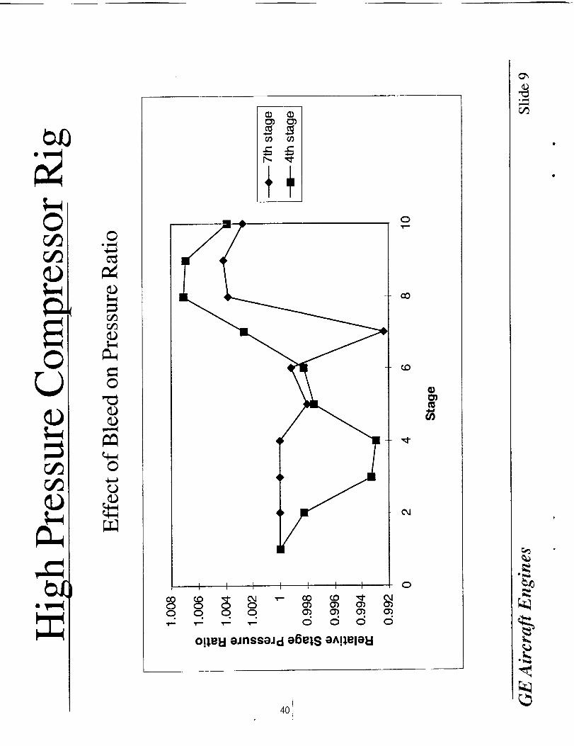
Figure (20) shows the relative difference in total pressure
at each stage based on the simulation used to generate the
results in Fig. (18) and (19) (i.e., best estimate of bleedrates, IGV and vane settings) and two other bleed rateschedules. The first of these bleed rate schedules, annotated
by shaded bars, corresponds to that used to generate the
results in Figs. (14) through (17). For this bleed schedule
the front end of the compressor becomes unloaded relative
to the back end. The next result, annotated _" open bars,
was generated by lowering the third stage bleed rate to thatmeasured. By drawing less third stage bleed air the pre-
dicted pressure ratio of the front stages increased to near
their measured values, while that of the back stages was
reduced. Finally, reducing the amount of bleed air being
dra_-n from the seventh stage bleed to that measured low-
ered the predicted pressure ratio of stages eight through tento near that measured. Stages one through four remained
unchanged as stage seven bleed was reduced; while stages
five through seven experienced an increase in pressure ra-
tio. The results shown in Fig. (20) are quite si_cant
for they clearly show how bleed can affect the matching of
stages _ithin a compressor. The initial simulation using
the a priori estimates of bleed rates was judged to be less
than satisfactory for design purposes. Clearly. in addition
to hax-ing sound models to account for the unsteady flow
field _-ithin axial flow multistage compressors, it i_ equally
important to have credible _-zimates of the leakage flowrates and the bleed flow rates.
A series of simulations were also performed to ascertain
APNASA's ability to compute the impact of throttling on
compressor performance. The wheel speed for these simula-
tions corresponds to that used in the previous simulations.
Figure (21) shows the percen_ difference in total pressure
ratio of individual stages relative to their predicted total
pressure ratio at the operating line (i.e., simulation results
used to generate the results in Fig. (18)). The pressure
ratio being defined from stator leading edge to rotor trail-
ing edge. For the tenth stage the pressure ratio is from
the leading edge of the ninth stage stator to compressor
discharge.
A series of simulations were executed for increasing back
pressure until the code failed to converge. The highest total
pressure ratio for which a converged solution was obtained
is less than the total pressure ratio at which the compressor
stalled. The first case labeled Case 1 is for a bark pressure
slightly greater than the value corresponding to Fig. (18),
while Case 4 is for a back pressure setting very close to
the numerical stall point. The other two cases are for back
pressure settings which lay ber_-een these two extremes.
For Case 1, the slight increase in back pressure caused
the last six stages to move slightly up their pressure charac-
teristic. The operating point of the first four stages remains
unchanged. Case 2 increased the back pressure further and
caused all of the stages with the exception of stage 1 to
respond. The mass flow, being set by the first stage, is un-
affected by this increase in bark pressure. The change in
the pressure ratio of stages fi_ through nine is significantly
greater than that for stage ten. Stage ten show a modest
change in pressure ratio which implies that it is operating
on the flat part of its characteristic. Raising the back pres-
sure still higher, Case 3, further increases the pressure ratio
of stages three through nine. Stages one and two remain
unchanged as does the mass flow, while the pressure ratio
across stage 10 decreases. Stage ten is operating on thepositive side of its pressure characteristic. Throttling the
compressor to near its numerical stall point, Case 4, causes
an increase in pressure ratio of stages two through eight.
The pressure ratio for stage one remains unchanged as does
the mass flow. The pressure ratio for stages nine and ten
has decreased. Both nine and ten are now operating on
the positive side of their characteristic. The decrease in
stage ten's pressure ratio from its previous value is quite
noticeable. It appears that the pressure characteristic forstage ten rolls over very abruptly after peak pressure. Ob-
taining a converged solution at still higher back pressuresproved difficult because of the extreme sensitivity to back
pressure setting. It is thought that stage eight is operat-
ing near peak pressure and that any slight increase in back
81
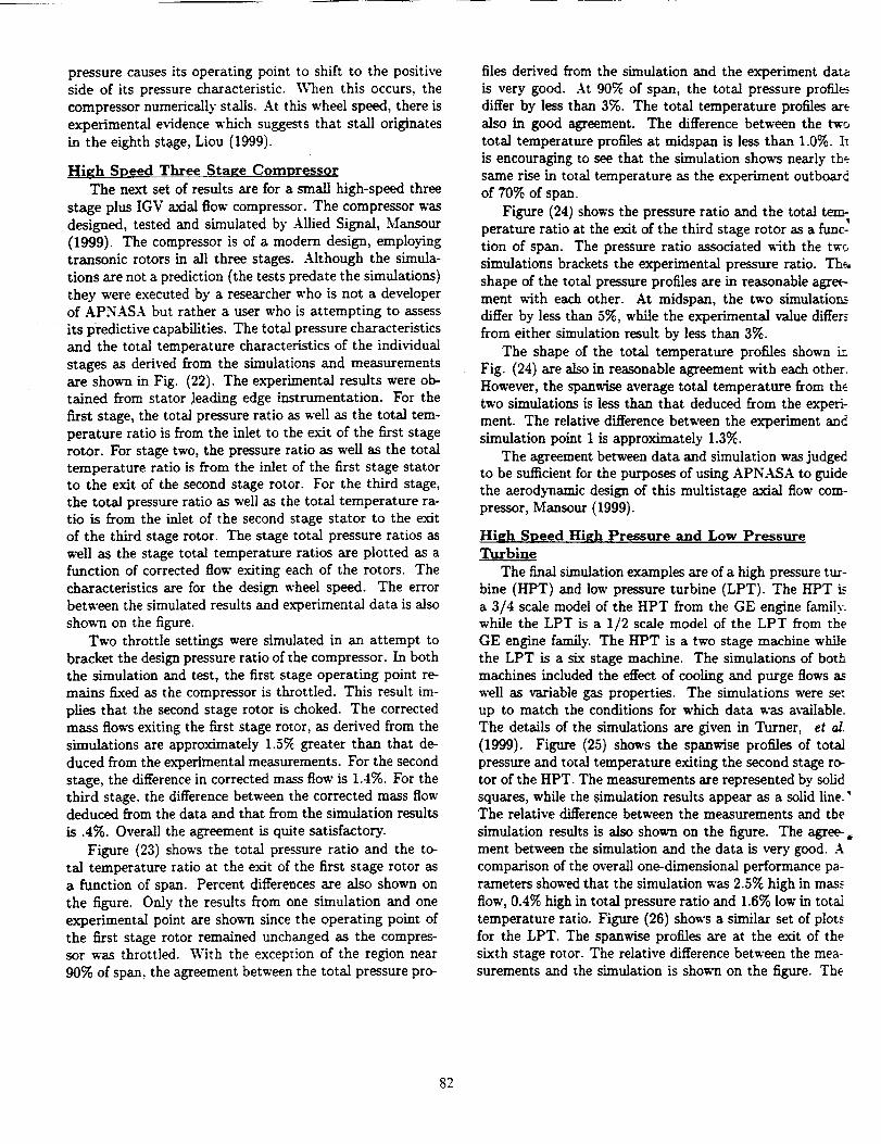
pressurecauses its operating point to shift to the positive
side of its pressure characteristic. I_Then this occurs, the
compressor numerically stalls. At this wheel speed, there is
experimental evidence which suggests that stall originates
in the eighth stage, Liou (1999).
High Speed Three Stage Compressor
The next set of results are for a small high-speed three
stage plus IGV axial flow compressor. The compressor was
designed, tested and simulated by Allied Signal, Mansour
(1999). The compressor is of a modern design, employing
transonic rotors in all three stages. Although the simula-
tions are not a prediction (the tests predate the simulations)
they were executed by a researcher who is not a developerof APNASA but rather a user who is attempting to assess
its predictive capabilities. The total pressure characteristicsand the total temperature characteristics of the individual
stages as derived from the simulations and measurementsare shown in Fig. (22). The experimental results were ob-
tained from stator :leading edge instrumentation. For the
first stage, the total pressure ratio as well as the total tem-
perature ratio is from the inlet to the exit of the first stage
rotor. For stage two, the pressure ratio as well as the totaltemperature ratio is from the inlet of the first stage stator
to the exit of the second stage rotor. For the third stage,
the total pressure ratio as well as the total temperature ra-
tio is from the inlet of the second stage stator to the exit
of the third stage rotor. The stage total pressure ratios as
well as the stage total temperature ratios are plotted as afunction of corrected flow exiting each of the rotors. The
characteristics are for the design wheel speed. The error
between the simulated results and experimental data is also
shown on the figure.
Two throttle settings were simulated in an attempt to
bracket the design pressure ratio of the compressor. In both
the simulation and test, the first stage operating point re-
mains fixed as the compressor is throttled. This result im-
plies that the second stage rotor is choked. The corrected
mass flows exiting the first stage rotor, as derived from the
simulations are approximately 1.5_ greater than that de-
duced from the experimental measurements. For the second
stage, the difference in corrected mass flow is 1.4%. For thethird stage, the difference between the corrected mass flowdeduced from the data and that from the simulation results
is .4%. Overall the agreement is quite satisfactory.
Figure (23) shows the total pressure ratio and the to-
tal temperature ratio at the exit of the first stage rotor as
a function of span. Percent differences are also shown on
the figure. Only the results from one simulation and one
experimental point are shown since the operating point of
the first stage rotor remained unchanged as the compres-
sor was throttled. With the exception of the region near
90% of span, the agreement between the total pressure pro-
files derived from the simulation and the experiment data
is very good. At 90% of span, the total pressure profil_
differ by less than 3%. The total temperature profiles are
also in good agreement. The difference between the tw_
total temperature profiles at midspan is less than 1.0%. I,.
is encouraging to see that the simulation shows nearly the
same rise in total temperature as the experiment outboardof 70% of span.
Figure (24} shows the pressure ratio and the total tem-
perature ratio at the exit of the third stage rotor as a func-'
tion of span. The pressure ratio associated with the tw_
simulations brackets the experimental pressure ratio. The.
shape of the total pressure profiles are in reasonable agree-ment with each other. At midspan, the two simulatiom
differ by less than 5%, while the experimental value differ._
from either simulation result by less than 3%.
The shape of the total temperature profiles shown i:
Fig. (24) are also in reasonable agreement with each other.
However, the spanwise average total temperature from the
two simulations is less than that deduced from the experi-
ment. The relative difference between the experiment and
simulation point 1 is approximately 1.3%.
The agreement between data and simulation was judgedto be sufficient for the purposes of using APNASA to guide
the aerodynamic design of this multistage axial flow com-
pressor, Mansour (1999).
High SoeedHi_h Pressure and Low Pressure
Turbine
The final simulation examples are of a high pressure tur-bine (HPT) and low pressure turbine (LPT). The HPT i_
a 3/4 scale model of the HPT from the GE engine family.while the LPT is a 1/2 scale model of the LPT from the
GE engine family. The HPT is a two stage machine while
the LPT is a six stage machine. The simulations of both
machines included the effect of cooling and purge flows as
well as variable gas properties. The simulations were se_
up to match the conditions for which data was a_-ailable.
The details of the simulations are given in Turner, et oi.
(1999). Figure (25) shows the spanwise profiles of total
pressure and total temperature exiting the second stage ro-
tor of the HPT. The measurements are represented by solid
squares, while the simulation results appear as a solid line."The relative difference between the measurements and the
simulation results is also shown on the figure. The agree-_ment between the simulation and the data is very good. A
comparison of the overall one-dimensional performance pa-
rameters showed that the simulation was 2.5% high in mas.,
flow, 0.4% high in total pressure ratio and 1.6% low in total
temperature ratio. Figure (26) show's a similar set of plots
for the LPT. The spanwise profiles are at the exit of the
sixth stage rotor. The relative difference between the mea-
surements and the simulation is shown on the figure. The
82

agreementbetweenthetwoisalsoverygood.FortheLPTstudy,a comparisonof theoverallone-dimensionalperfor-manceparametersshowedthatthesimulationwas2.5%lowinmassflow,0.3%highin totalpressureratio,and3.5%lowin total temperatureratio.
Themachineswhosesimulationresultswerepresentedin thissectioncovera broadrangeof multistageaxialflowturbomachineryconfigurations.Theobjectiveof thissec-tionwasto illustrateto theturbomachinerydesigncommu-nity what could be, and what could not be, predicted by a
code based on the average-passage flow model with the cur-
rent procedures to account for the effects of the unsteady
flow environment within multistage turbomachines. All thesimulations were executed without recourse to information
supplied by external models or data which prescribed the
aerodynamic matching of stages, this information being an
output of the simulations and not an input. Being able
to reliably establish the aerodynamic matching of stages in
a multistage configuration is critical to ensuring that ad-
vanced designs attain their aerodynamic goals in the firstbuild.
In the next section the current state of the art for sim-
ulating multistage axial flow turbomachines in support ofaerodynamic design using models which are uncoupled from
through-flow models is summarized. Suggestions for future
work are also presented.
Summary and Suggested Future Work
Before summarizing it is important to stress the need
to have correct geometry and correct inflow and outflow
boundary conditions before attempting any simulation.
This detail cannot be emphasized enough as evidenced
by the findings of Shabbir, et al. (1997), Escuret and
Veysseyre, (1997), Wellborn, et al. (1999). It is impor-
tant to know the geometry at the flow conditions being
simulated. This includes the blade geometry as well as the
hub and shroud geometry. Rotor tip clearance, stator hub
clearance, variable geometry setting, and variable geome-try button configuration must all be known. Blade fillet
geometry and surface finish must also be known. All cav-ities which are opened to the primary flow path must be
known. All leakage flows must be known including those
associated with shrouded blading, bleed flows, purge flows
and the cooling flows of cooled turbines. If any of these
details (geometD', inflow and outflow boundary, conditions)
are unknown, it is important to establish the sensitivity ofthe simulation results to their assumed values.
Table I is a bullet chart which summarizes the fluid me-
chanics addressed in this paper. At the top of the list is
spanwise transport of wake fluid particles which leads to a
redistribution of total temperature, and momentum. Al-
though not specifically addressed, the spanwise redistribu-
tion of entropy is also implied.
Next on the list is circumferential transport of wake fluid
particles which also leads to a redistribution of total tem-
perature and momentum. The flow physics associated with
this redistribution was shown to be equivalent to that as-
sociated with spanwise redistribution of total temperature.
Although circumferential redistribution of total tempera-
ture does not appear to impact aerodynamic performance,
it does lead to total temperature segregation resulting in the
formation of hot spots. These hot spots have a significant
impact on turbine blade life.
TABLE I
Summary of Unsteady Deterministic Flow ProcessesDiscussed Which Impact The Time-Average
Performance of Multistage Turbomachinery
• Spanwise transport of wake fluid particles.
• Circumferential transport of wake fluid particles.
• The strainingof wakes.
I
Circumferential redistribution of momentum also in-
volves the interaction between a blade and incoming wakes
and blade boundary layers. The impact of incoming wakes
interacting with turbulent blade boundary layers on aero-dynamic performance is not clear. There appears to be an
indication that the interaction of compressor rotor tip clear-ance flows with a downstream stator leads to increased loss.
However, when the interaction involves a transitional blade
boundary l_'er, evidence exists that aerodynamic perfor-
mance is impacted. This subject will be addressed later inthis section.
Next on the chart is the straining of wakes as they con-
vect through a blade row. This straining process leads to
wake recovery. Wake recovery results in the transfer of en-
ergy by a reversible flow process between the unsteady flow
generated by wakes and the time average flow field. Wake
recovery was sho_na to impact the mixing loss of wakes as
they pass through a do_aastream blade row. With respectto an axial flow compressor, the mi.-dng loss attributed to
2D wakes is significantly reduced by the wake recovery pro-
cess. For an axial flow turbine, the mixing loss attributed to2D wakes is increased by the wake recovery process. Thus,
there is a performance benefit to be gained in axial flow
compressors by having blade rows closely spaced, while the
opposite is true for axial flow turbines.
It was shown that the wake recovery process also im-
pacted the pressure rise across the blade row through which
the wakes are passing. The pressure rise was linked to flow
blockage defined in terms of an ener_" recovery thickness.
83

1.0 .
I!! ,,0.0 - m
I
I I ,= i i i I I I i i
-0.5 1 2 3 4 5 6 7 8 9 10
ROTOR TRAILINGEDGE STATION
Fig. 14a. Comparison of total temperature as predicted by
APNASA and CAFMIX II for the 10-stage GE90 compres-
sor.
lOO.O
80.0
L
60.0
D_ •
0_ 4oo _.37O/o]
0.0 • • •
P_RATIO
-- APNASA• CAFMIX II
Fig. 15a. Spanwise distribution of total pressure at the exit
of the stage 3 stator in the GEg0 compressor.
100 - = .
• -- APNASA
6080_ • [ •CAFMIXIIz
m
¢n 2"7% I
0
P, RATIO - "
Fig. 15c. SpanwJse distribution of total pressure at the exit
of the stage 7 stator in the GE90 compressor.
5,0
4.0
_ .0
_ 2.0
i.oio_
o.o
-1.oI i i i i I I i 1 I01 2 3 4 5 6 7 8 9 1
ROTOR TRAILING EDGE STATION
Fig. i4b. Comparison of total pressure as predicted by AP-
NASA and CAFMIX H for the 10-stage GE90 compressor.
,0oj
60 F-
140 F
I
j-
ol
lOO
I°°f40_
2O
--'O _PF_IISXI,
T,RATIO
Fig. 15b. Spanwise distribution of total temperature at the
exit of the stage 3 stator in the GEg0 compressor.
1-- APNASA .
• CAFMIX II
oT, RATIO
Fig. 15d. Spanwise distribution of total temperature at the
exit of the stage 7 stator in the GEg0 compressor.
84

Z
O.
too %
8O
-- APNASA
• CAFMIX II6O
4O
20
o #
P, RATIO
Fig. 15e. Spanwise distribution of total pressure at the
compressor exit in the GE90 compressor.
Z<(3_o)
0.95
APNASA
CAFMIX II
0.90
0.851 2 3 4 5 6 7 8 9 10
ROTOR TRAILING EDGE STATION
Fig. 16. Flow blockage distribution through the GE90 com-
pressor.
100
90
80
7O
6Oz<o. 5003
4O
30
20
10
05
-- APNASA
• CAFMIX II
i I I _ II
10 15 20 25 30 35
ABSOLUTE FLOW ANGLE (DEGS)
Fig. 171). Absolute flow angle at the exit of the stage 3
stator in the GE90 compressor.
100
80
6O
40
2O
-- APNASA
• CAFMIX II
0' _ " I _
T, RATIO
Fig. 15e. Spanwise distribution of total pressure at the
compressor exit in the GE90 compressor.
100
9O
80
70
60
50
40
30
20
10
025
L APIASA ' ' e__
' ' 4'0 '30 35 4 50 55
RELATIVE FLOW ANGLE (DEGS)
Fig. 17a. Relative flow angle at the exit of the stage 3 rotor
in the GE90 compressor.
100
,o!
80 F _APNASA •
I50
40
30
10
0 -- .....
20 25 30 35 40 45 50
RELATIVE FLOWANGLE(DEGS)
Fig. 17c. Relative flow angle at the exit of the stage 7 rotor
in the GE90 compressor.
85

100
90
80
70
60
5O
40
3O
20
z _ APNASA< •o.. • CAFMIX IIf.D
IP9 ,00 5 -10 15 20 25 30
ABSOLUTE FLOW ANGLE (DEGS)
Fig. 17d. Absolute flow angle at the exit of the stage 7stator in the GEg0 compressor.
3.0
_O 2.0 DIFFERENCE = 1 - Ptam_'sAI'- P_::,ATA
CC
UJO'-1.0 _
_ 0.0 _
_z
O -1.0
t,r
N -2.0
_3_0
0 1 2 3 4 5 6 7 8 9 10
STAGE NUMBER
Fig. 18. Percent difference in total pressure through theGE90 compressor near the design speed operating point.
100
z<
8O
60
4O
20
-- APNASA
•e/e e • • DATA
OO
100
Pt RATIO
Fig. lga. $panwise distribution of total pressure at the exit
of the stage 3 rotor in the GE90 near design speed.
100
80
6O
N 4O
2O
80
6OZ
4O
2O
100
-- APNASA
• • DATA 80
60
• 40
20
2"52°/' I_]
P_RATIO
Fig. 19c. Spanwise distribution of total pressure at the exitof the stage 7 rotor in the GE90 near design speed.
--APNASA
• DATA
T, RATIO
Fig. 19b. Spanwise distribution of total temperature at the
exit of the stage 3 rotor in the GE90 near design speed.
--. A
0
1-,RATIO
Fig. 19d. Spanwise distribution of total pressure at the exit
of the stage ? rotor in the GE90 near design speed.
86
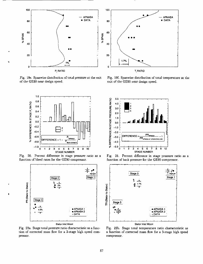
100 100J
Z<C(3.o')
80
60
4O
2O
-- APNASA
• DATA
P=RATIO
Fig. 19e. Spanwise distribution of total pressure at the exitof the GE90 near design speed.
8O
60Z
I1.o3
40
20
0 i
- APNASA
• DATA
T,RATIO
Fig. 19£ Spanwise distribution of total temperature at theexit of the GE90 near design speed.
1.0
O 0.8I--< 0.6rr
_'- 0.4UJ
c_< 0.2
f/)
z o.oILl
-0.2ZuJrr -0.4UJLL
-u- -0.6GI
-0.8
-1.00
½21
DIFFERENCE = 1
i I i i i
1 2 3 4 5
PtARNASA II
i i i i I
6 7 8 9 10
STAGE NUMBER
Fig. 20. Percent difference in stage pressure ratio as afunction of bleed rates for the GE90 compressor.
t__0
o
fD
E
___r_• 3%
_• -.I.-4.5% i •APNASA1
B APNASA2+ "-r-
÷ DATA
Stator Inlet Wcorr
Fig. 22a. Stage total pressure ratio characteristic as a func-tion of corrected mass flow for a 3-stage high speed com-pressor.
O 5.0
4.0W
rr 3.0cO(_ 2.0UJ
a. 1.0UJ(3< 0.0
_z -1.0LUo -2.0ZWrr -3.0UJtJ." -4.0
-5.00
Fig. 21.
1
DIFFERENCE- PR*_A - 1P R *_'_ASX AT OPERA'I3NG UNE
STAGE NUMBER
Percent difference in stage pressure ratio as afunction of back pressure for the GEg0 compressor.
0Io
fl:I--
; Stage 2
Stage 1
j 1.1%
Stage 3
4I• _t_ • APNASA 1+ 5.8% ' • APNASA 2
T i + DATA
, J , L , i , i , i ,
Stator Inlet Wcorr
Fig. 22b. Stage total temperature ratio characteristic asa function of corrected mass flow for a 3-stage high speedcompressor.
87
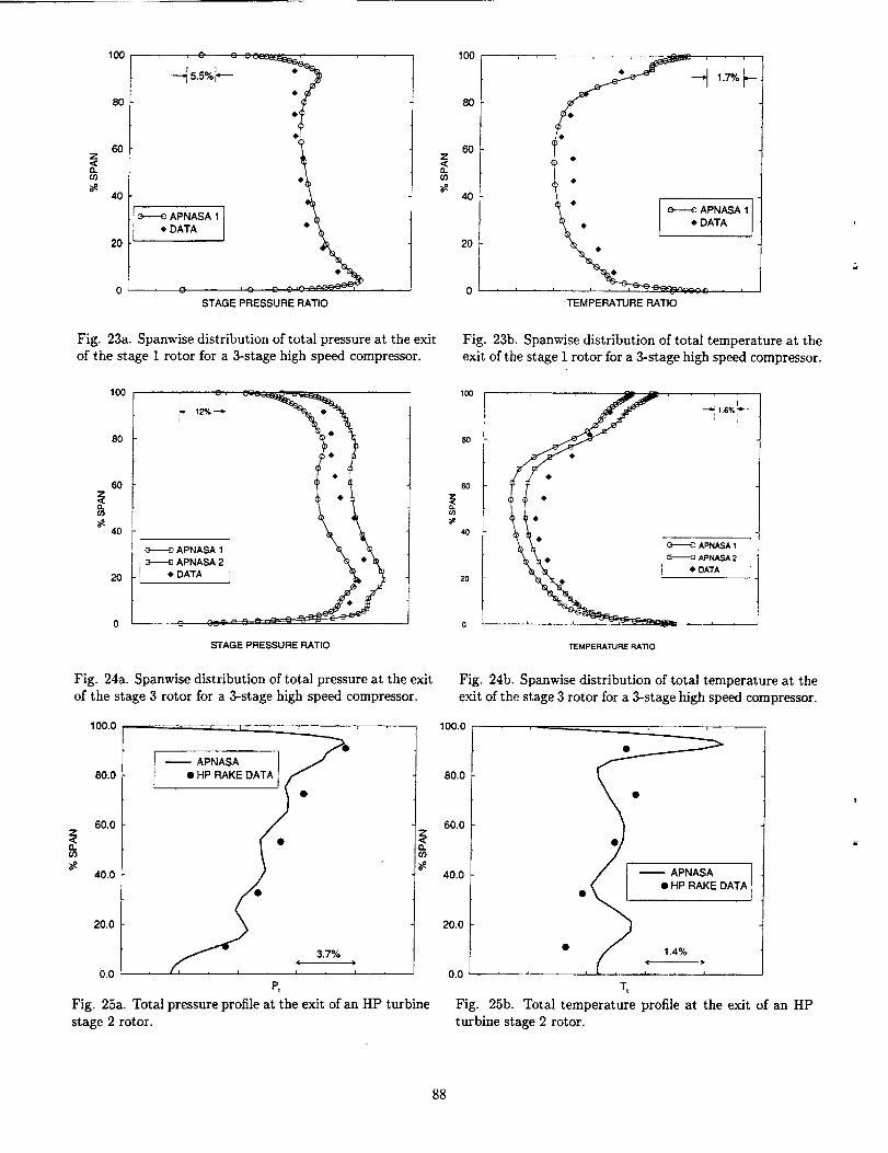
100
8O
6O
4O
20
, 0 0 ,C,- " , •
@
i
i
APNASA 1 t
• DATA
' C " ' C _ + -
STAGE PRESSURE RATIO
Fig. 23a. Spanwise distribution of total pressure at the exitof the stage 1 rotor for a 3-stage high speed compressor.
10o
80 _ PNASA
60
N40
20
0
STAGE PRESSURE RATIO
Fig. 24a. Spanwise distribution of total pressure at the exit
of the stage 3 rotor for a 3-stage high speed compressor.
z<(3.
100.0 .' , .............. ,
-- APNASA ] _"
80.0
60.0 ZCLO)
40.0
20.0
f ( •3.7°/,,
0.0 , J I i I i l i I i
Pt
Fig. 25a. Total pressure profile at the exit of an ttP turbine
stage 2 rotor.
z,<i"1
10o
80
60
4O
20
TEMPERATURE RATIO
Fig. 23b, Spanwise distribution of total temperature at the
exit of the stage 1 rotor for a 3-stage high speed compressor.
I00
80
60
4O
2O
80.0
60.0
40.0
20.0
i ["-_1.6% ""
APNASAI
APNASA2DATA !
TEMPERATURE RATIO
Fig. 24b. Spanwise distribution of total temperature at theexit of the stage 3 rotor for a 3-stage high speed compressor.
100.0 , ,
• •
• / 1.4+/o
0.0 ....
T,
Fig. 25b. Total temperature profile at the exit of an HPturbine stage 2 rotor.
88

100.0
80.0
60.0
40.0
20.0
0.0
' t •
2.3%(
, i ,
PN A• I__P.._KEOATA
PI
Fig. 26a. Total pressure profile at the exit of an LP turbine.
5
t
z<e_co
100.0
80.0
60.0
40.0
20.0
0.0
i<; _o
• °I j m AP.AsAoi t '""A_:::$oAT,
1.8% . • 0 0
Fig. 26b. Total temperature profile at the exit of an LP
turbine.
0.70
0.65
0.60
c
"2 0.55
0
o 0.50
0.45
0.40
0.350.25 0.30 0.35 0.40 0.45 0.50
Inlet Row Coefficient
Fig. 27. Steady flow through a cascade with blockage.
Fig. 28. Overall pressure coefficient as a function of inlet
flow coefficient for the NASA-Lewis four stage axial flow
compressor.
89

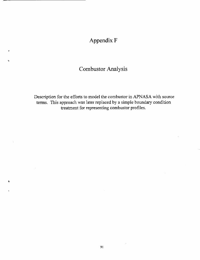
Appendix F
Combustor Analysis
Description for the efforts to model the combustor in APNASA with source
terms. This approach was later replaced by a simple boundary condition
treatment for representing combustor profiles.
91

GE90 Full Engine Simulation
COMBUSTOR ANALYSIS
An attempt was made to include the combustor in a reduced APC analysis of the
GE90. The reduced APC analysis included the outlet guide vane (OGV) of the high pressure
compressor, diffuser and combustor section, and first stage nozzle of the high pressure
turbine (HPT). The flowpath included the diffuser and the hot section of the combustor, as
illustrated by the heavy line in Fig. I. The APC analysis was for two blade rows, the OGV
and HPT nozzle, but the axisymmetric grid included the diffuser and combustor flowpaths, as
shown in Fig. 2. Typical blade-to-blade grids for the OGV and HPT nozzle are shown in Figs.
3 and 4, respectively. The effect of the combustor was modeled with average passage bodyforces.
,a
The body forces for the combustor section were obtained from a separate computa-
tion of the combustor flowfield using the program CONCERT3D, one of GE's combustion
CFD codes. The three-dimensional solution from CONCERT3D was circumferentially
averaged and interpolated onto the APC axisymmetric grid, as shown in Fig. 5. This
axisymmetric solution was used to compute APC body forces by running the solution through
the APC axisymmetric residual computation. With the body forces computed in this manner,
it was thought that this axisymmetric solution would be recovered in the APC solution
procedure. Part of the problem also stems from the fact that the governing equations,
discretization schemes, and solution procedures for CONCERT3D and APC are very differ-
ent, which makes it difficult to obtain consistent body forces to couple the solutions.
APC was subsequently used to compute the solution of the two blade row system
with the combustor body forces obtained as described above. Several shortcomings in this
approach were identified. Since the capability does not currently exist to model the diffuser,
the rate and distribution of the flow aft of the OGV was inaccurate. Consequently, the desired
effect of the body forces was not achieved. To obtain the proper effect with the body forces,
the mass flow rate distribution must be approximately the same as the original distribution
from the CONCERT3D analysis. Without modeling all the geometric details of the combus-
tor, this would be very difficult to achieve.
It is believed that the shortcomings in the above approach could be overcome with
much additional effort. The approach has the advantage of the combustor contribution com-
ing from a detailed computation with a combustion CFD code. A much simpler, yet less
desirable, methodology for coupling the compressor and turbine is currently being developed
until the problems with the first approach can be overcome. The simpler method involves
coupling the compressor and turbine by iteratively adjusting the OGV exit boundary condi-
tions and HPT nozzle inlet boundary conditions based on the most recent solutions of each.
92
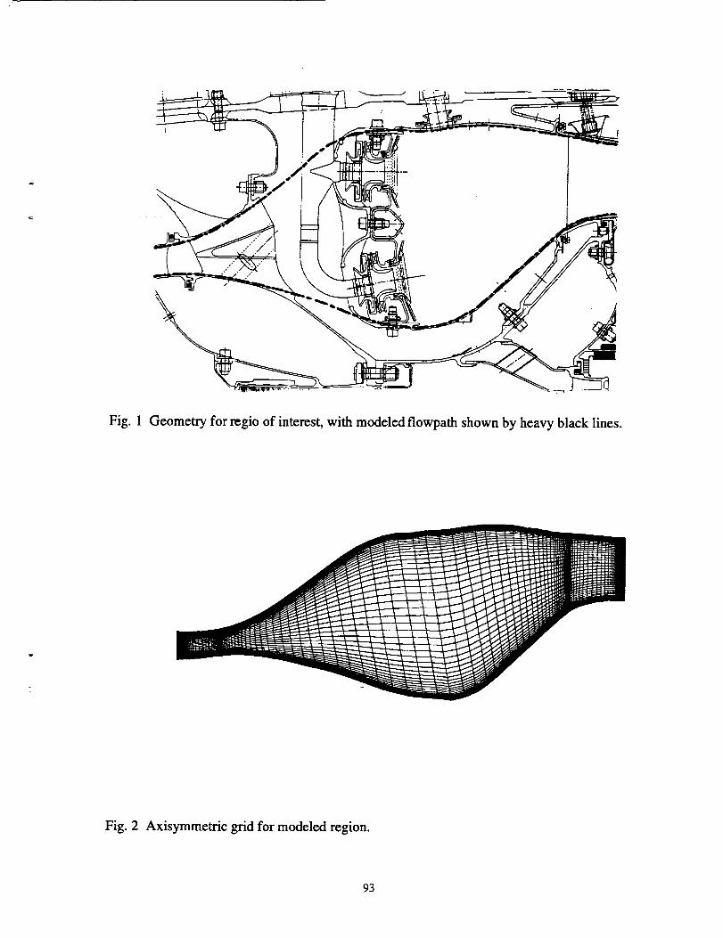
Fig. 1 Geometry for regio of interest, with modeled flowpath shown by heavy black lines.
Fig. 2 Axisymmetric grid for modeled region.
93

Fig. 3 Blade-to-bladegrid for compressorOGV.
Fig. 4 Blade-to-bladegrid for HPTnozzle.
94
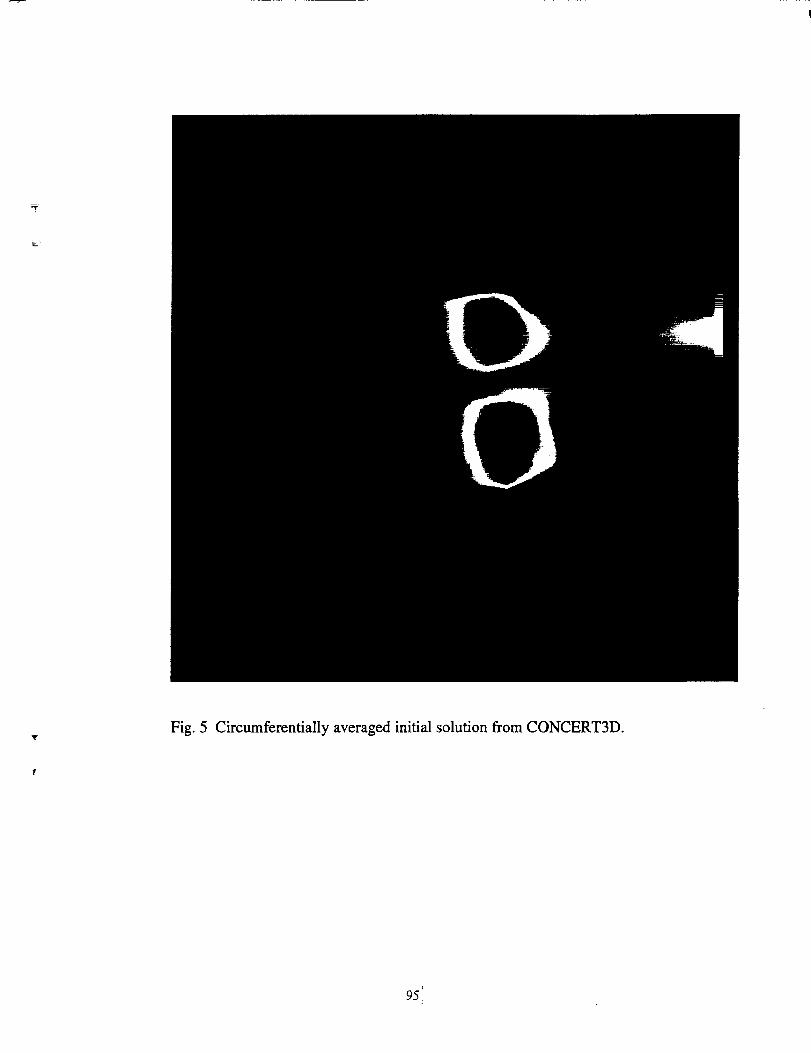
Fig. 5 Circumferentially averaged initial solution from CONCERT3D.
951

REPORT DOCUMENTATION PAGE FormApprovedOMB No. 0704-0188
Public reporting burden for this collection of information is estimated to average f hour per response, including the time for reviewing instructions, searching existing data sources,
gathering and maintaining the data needed, and completing and reviewing the collection of information. Send comments regarding this burden estimate or any other aspect of thiscollection of information, including suggestions for reducing this burden, to Washington Headquarters Services, Directorate for Information Operations and Reports. 1215 Jefferson
Davis Highway. Suite 1204, Arlington, VA 22202-4302, and to the Office of Management and Budget, Paperwork Reduction Project (0704-0188). Washington, DC 20503.
1, AGENCY USE ONLY (Leave blank)
4. TITLE AND SUBTITLE
2. REPORT DATE
March 2000
Full 3D Analysis of the GE90 Turbofan Primary Flowpath
6. AUTHOR(S)
Mark G. Turner
7. PERFORMING ORGANIZATION NAME(S) AND ADDRESS(ES)
GE Aircraft Engines
One Neumann Way
Cincinnati, Ohio 45215-6301
9. SPONSORING/MONITORING AGENCY NAME(S) AND ADDRESS(ES)
National Aeronautics and Space Administration
John H. Glenn Research Center at Lewis Field
Cleveland, Ohio 44135-3191
;3. REPORT TYPE AND DATES COVERED
Final Contractor Report
5. FUNDING NUMBERS
WU-509-10-11-130NAS 3-26617
Task Order 65
8. PERFORMING ORGANIZATIONREPORT NUMBER
E-12205
10. SPONSORING/MONITORINGAGENCY REPORT NUMBER
NASA CR--2000-209951
11. SUPPLEMENTARY NOTES
Pr_ectManager, Joseph P. Veres, Computing and Interdisciplinary Systems Office, organization code 2900,
(216)433--2436.
12a. DISTRIBUTION/AVAILABILITY STATEMENT
Unclassified - Unlimited
Subject Categories: 07, 02, and 34 Distribution: Nonstandard
This publication is available from the NASA Center for AeroSpace Information, (301) 62143390.
12b. DISTRIBUTION CODE
13. ABSTRACT (Maximum 200 words)
The multistage simulations of the GE90 turbofan primary flowpath components have been performed. The multistage
CFD code, APNASA, has been used to analyze the fan, fan OGV and booster, the 10-stage high-pressure compressor and
the entire turbine system of the GEg0 turbofan engine. The code has two levels of parallel, and for the 18 blade row full
turbine simulation has 87.3 percent parallel efficiency with 121 processors on an SGI ORIGIN. Grid generation is
accomplished with the multistage Average Passage Grid Generator, APG. Results for each component are shown which
compare favorably with test data.
14. SUBJECT TERMS
Turbofan; CFD; Modeling; Flow; Numerical; Compressor; Turbine
17. SECURITY CLASSIFICATION 18. SECURITY CLASSIFICATION 19. SECURITY CLASSIFICATIONOF REPORT OF THIS PAGE OF ABSTRACT
Unclassified Unclassified Unclassified
NSN 7540-01-280-5500
15, NUMBER OF PAGES
10t16. PRICE CODE
A0620, LIMITATION OF ABSTRACT
Standard Form 298 (Rev. 2-89)Prescribed by ANSI Std Z39-18
29B-102
#w
Recommended


