Financial Distress Prediction Model of Manufacturing
Industry Empirical Evidence from Shenzhen and Shanghai A-share Listed Firms
Lan Wu
Business School of Sichuan University
Chengdu, China
Pan Wan
Business School of Sichuan University
Chengdu, China
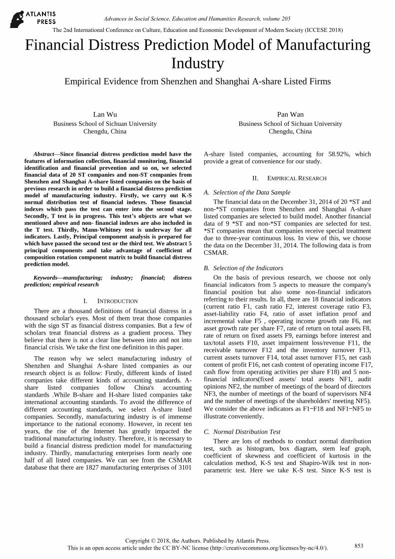
Abstract—Since financial distress prediction model have the
features of information collection, financial monitoring, financial
identification and financial prevention and so on, we selected
financial data of 20 ST companies and non-ST companies from
Shenzhen and Shanghai A-share listed companies on the basis of
previous research in order to build a financial distress prediction
model of manufacturing industry. Firstly, we carry out K-S
normal distribution test of financial indexes. Those financial
indexes which pass the test can enter into the second stage.
Secondly, T test is in progress. This test’s objects are what we
mentioned above and non- financial indexes are also included in
the T test. Thirdly, Mann-Whitney test is underway for all
indicators. Lastly, Principal component analysis is prepared for
which have passed the second test or the third test. We abstract 5
principal components and take advantage of coefficient of
composition rotation component matrix to build financial distress
prediction model.
Keywords—manufacturing; industry; financial; distress
prediction; empirical research
I. INTRODUCTION
There are a thousand definitions of financial distress in a thousand scholar's eyes. Most of them treat those companies with the sign ST as financial distress companies. But a few of scholars treat financial distress as a gradient process. They believe that there is not a clear line between into and not into financial crisis. We take the first one definition in this paper.
The reason why we select manufacturing industry of Shenzhen and Shanghai A-share listed companies as our research object is as follow: Firstly, different kinds of listed companies take different kinds of accounting standards. A-share listed companies follow China's accounting standards .While B-share and H-share listed companies take international accounting standards. To avoid the difference of different accounting standards, we select A-share listed companies. Secondly, manufacturing industry is of immense importance to the national economy. However, in recent ten years, the rise of the Internet has greatly impacted the traditional manufacturing industry. Therefore, it is necessary to build a financial distress prediction model for manufacturing industry. Thirdly, manufacturing enterprises form nearly one half of all listed companies. We can see from the CSMAR database that there are 1827 manufacturing enterprises of 3101
A-share listed companies, accounting for 58.92%, which provide a great of convenience for our study.
II. EMPIRICAL RESEARCH
A. Selection of the Data Sample
The financial data on the December 31, 2014 of 20 *ST and non-*ST companies from Shenzhen and Shanghai A-share listed companies are selected to build model. Another financial data of 9 *ST and non-*ST companies are selected for test. *ST companies mean that companies receive special treatment due to three-year continuous loss. In view of this, we choose the data on the December 31, 2014. The following data is from CSMAR.
B. Selection of the Indicators
On the basis of previous research, we choose not only financial indicators from 5 aspects to measure the company's financial position but also some non-financial indicators referring to their results. In all, there are 18 financial indicators (current ratio F1, cash ratio F2, interest coverage ratio F3, asset-liability ratio F4, ratio of asset inflation proof and incremental value F5 , operating income growth rate F6, net asset growth rate per share F7, rate of return on total assets F8, rate of return on fixed assets F9, earnings before interest and tax/total assets F10, asset impairment loss/revenue F11, the receivable turnover F12 and the inventory turnover F13, current assets turnover F14, total asset turnover F15, net cash content of profit F16, net cash content of operating income F17, cash flow from operating activities per share F18) and 5 non-financial indicators(fixed assets/ total assets NF1, audit opinions NF2, the number of meetings of the board of directors NF3, the number of meetings of the board of supervisors NF4 and the number of meetings of the shareholders' meeting NF5).
We consider the above indicators as F1—F18 and NF1—NF5 to
illustrate conveniently.
C. Normal Distribution Test
There are lots of methods to conduct normal distribution test, such as histogram, box diagram, stem leaf graph, coefficient of skewness and coefficient of kurtosis in the calculation method, K-S test and Shapiro-Wilk test in non-parametric test. Here we take K-S test. Since K-S test is
The 2nd International Conference on Culture, Education and Economic Development of Modern Society (ICCESE 2018)
Copyright © 2018, the Authors. Published by Atlantis Press. This is an open access article under the CC BY-NC license (http://creativecommons.org/licenses/by-nc/4.0/).
Advances in Social Science, Education and Humanities Research, volume 205
853
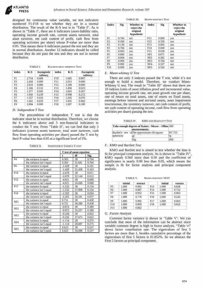
designed for continuous value variable, we test indicators numbered F1-F18 to see whether they are in a normal distribution. The result of the K-S test is in "Table I". As is shown in "Table I", there are 6 indicators (asset-liability ratio, operating income growth rate, current assets turnover, total asset turnover, net cash content of profit, cash flow from operating activities per share) whose P-value are more than 0.05. That means these 6 indicators passed the test and they are in normal distribution. Another 12 indicators should be culled because they do not pass the test and they are not in normal distribution.
TABLE I. KOLMOGOROV-SMIRNOV TEST
D. Independent T Test
The precondition of independent T test is that the
indicator must be in normal distribution. Therefore, we choose
the 6 indicators above and 5 non-financial indicators to
conduct the T test. From "Table II", we can find that only 3
indicators (current assets turnover, total asset turnover, cash
flow from operating activities per share) passed the T test by
their P-value less than 0.05 at a significant level of 5%.
TABLE II. INDEPENDENT SAMPLE T-TEST
T test of mean equation
t df Sig.
F4 the variance is equal 0.303 38 0.764
the variance isn’t equal 0.303 31.641 0.764
F6 the variance is equal -1.428 38 0.161
the variance isn’t equal -1.428 31.438 0.163
F14 the variance is equal -2.678 38 0.011
the variance isn’t equal -2.678 32.144 0.012
F15 the variance is equal -4.021 38 0.000
the variance isn’t equal -4.021 26.049 0.000
F17 the variance is equal -1.532 38 0.134
the variance isn’t equal -1.532 37.008 0.134
F18 the variance is equal -2.202 38 0.034
the variance isn’t equal -2.202 26.241 0.037
NF1 the variance is equal 0.751 38 0.458
the variance isn’t equal 0.751 36.289 0.458
NF2 the variance is equal -0.872 38 0.389
the variance isn’t equal -0.872 35.237 0.389
NF3 the variance is equal -0.226 38 0.822
the variance isn’t equal -0.226 37.675 0.822
NF4 the variance is equal -1.114 38 0.272
the variance isn’t equal -1.114 28.697 0.275
NF5 the variance is equal 0.623 38 0.537
the variance isn’t equal 0.623 36.088 0.537
TABLE III. MANN-WHITNEY TEST
Index Sig Whether to
reject the
original
hypothesis
Index Sig Whether to
reject the
original
hypothesis
F1 0.766 not F11 0.000 yes
F2 0.160 not F12 0.330 not
F3 0.130 not F13 0.003 yes
F4 0.766 not F14 0.040 yes
F5 0.003 yes F15 0.030 yes
F6 0.006 yes NF1 0.871 not
F7 0.004 yes NF2 0.382 not
F8 0.000 yes NF3 0.704 not
F9 0.000 yes NF4 0.337 not
F10 0.000 yes NF5 0.550 not
E. Mann-whitney U Test
There are only 3 indexes passed the T test, while it’s not enough to build a model. Therefore, we conduct Mann-Whitney U test. The result in "Table III" shows that there are 10 indexes (ratio of asset inflation proof and incremental value, operating income growth rate, net asset growth rate per share, rate of return on total assets, rate of return on fixed assets, earnings before interest and tax/total assets, asset impairment loss/revenue, the inventory turnover, net cash content of profit, net cash content of operating income, cash flow from operating activities per share) passing the test.
TABLE IV. KMO AND BARTLETT TEST
Take enough degrees of Kaiser - Meyer – Olkin
measurements.
.560
Bartlett's test of sphericity
The approximate chi-square 307.755
df 78
Sig. .000
F. KMO and Bartlett Test
KMO and Bartlett test is aimed to test whether the data is fit for principal component analysis. As is shown in "Table IV", KMO equals 0.560 more than 0.50 and the coefficient of significance is nearly 0.00 less than 0.05, which means the sample is fit for factor analysis and principal component analysis.
TABLE V. MANN-WHITNEY TEST
initial extract initial extract
F5 1.000 0.902 F13 1.000 0.836
F6 1.000 0.887 F14 1.000 0.732
F7 1.000 0.953 F15 1.000 0.863
F8 1.000 0.778 F16 1.000 0.542
F9 1.000 0.905 F17 1.000 0.665
F10 1.000 0.899 F18 1.000 0.816
F11 1.000 0.862
G. Factor Analysis
Common factor variance is shown in "Table V". We can conclude that most of the information can be abstract since variable common degree is high in factor analysis. “Table VI” shows factor contribution rate. The eigenvalues of first 5 factors are more than 1, besides cumulative percentage of the eigenvalues of first 5 factors is 81.852%. So we abstract the First 5 factors as principal component.
index K-S Asymptotic
saliency
index K-S Asymptotic
saliency
F1 2.754 0.000 F10 1.685 0.007
F2 2.458 0.000 F11 2.053 0.000
F3 2.619 0.000 F12 2.298 0.000
F4 1.166 0.132 F13 1.494 0.023
F5 1.377 0.045 F14 1.003 0.267
F6 1.030 0.239 F15 0.998 0.272
F7 1.557 0.016 F16 1.295 0.070
F8 1.432 0.033 F17 1.855 0.002
F9 2.884 0.000 F18 1.097 0.180
Advances in Social Science, Education and Humanities Research, volume 205
854
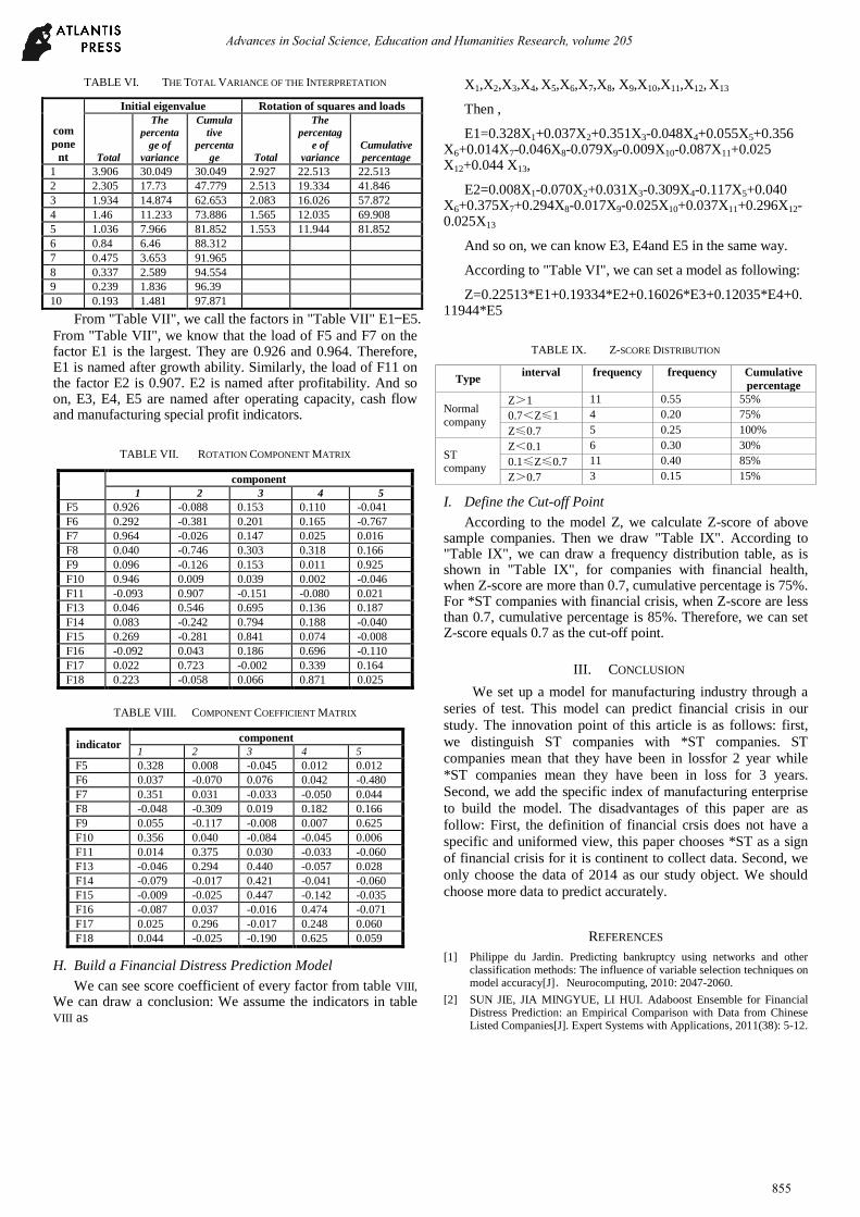
TABLE VI. THE TOTAL VARIANCE OF THE INTERPRETATION
com
pone
nt
Initial eigenvalue Rotation of squares and loads
Total
The
percenta
ge of
variance
Cumula
tive
percenta
ge Total
The
percentag
e of
variance
Cumulative
percentage
1 3.906 30.049 30.049 2.927 22.513 22.513
2 2.305 17.73 47.779 2.513 19.334 41.846
3 1.934 14.874 62.653 2.083 16.026 57.872
4 1.46 11.233 73.886 1.565 12.035 69.908
5 1.036 7.966 81.852 1.553 11.944 81.852
6 0.84 6.46 88.312
7 0.475 3.653 91.965
8 0.337 2.589 94.554
9 0.239 1.836 96.39
10 0.193 1.481 97.871
From "Table VII", we call the factors in "Table VII" E1—E5.
From "Table VII", we know that the load of F5 and F7 on the factor E1 is the largest. They are 0.926 and 0.964. Therefore, E1 is named after growth ability. Similarly, the load of F11 on the factor E2 is 0.907. E2 is named after profitability. And so on, E3, E4, E5 are named after operating capacity, cash flow and manufacturing special profit indicators.
TABLE VII. ROTATION COMPONENT MATRIX
component
1 2 3 4 5
F5 0.926 -0.088 0.153 0.110 -0.041
F6 0.292 -0.381 0.201 0.165 -0.767
F7 0.964 -0.026 0.147 0.025 0.016
F8 0.040 -0.746 0.303 0.318 0.166
F9 0.096 -0.126 0.153 0.011 0.925
F10 0.946 0.009 0.039 0.002 -0.046
F11 -0.093 0.907 -0.151 -0.080 0.021
F13 0.046 0.546 0.695 0.136 0.187
F14 0.083 -0.242 0.794 0.188 -0.040
F15 0.269 -0.281 0.841 0.074 -0.008
F16 -0.092 0.043 0.186 0.696 -0.110
F17 0.022 0.723 -0.002 0.339 0.164
F18 0.223 -0.058 0.066 0.871 0.025
TABLE VIII. COMPONENT COEFFICIENT MATRIX
indicator component
1 2 3 4 5
F5 0.328 0.008 -0.045 0.012 0.012
F6 0.037 -0.070 0.076 0.042 -0.480
F7 0.351 0.031 -0.033 -0.050 0.044
F8 -0.048 -0.309 0.019 0.182 0.166
F9 0.055 -0.117 -0.008 0.007 0.625
F10 0.356 0.040 -0.084 -0.045 0.006
F11 0.014 0.375 0.030 -0.033 -0.060
F13 -0.046 0.294 0.440 -0.057 0.028
F14 -0.079 -0.017 0.421 -0.041 -0.060
F15 -0.009 -0.025 0.447 -0.142 -0.035
F16 -0.087 0.037 -0.016 0.474 -0.071
F17 0.025 0.296 -0.017 0.248 0.060
F18 0.044 -0.025 -0.190 0.625 0.059
H. Build a Financial Distress Prediction Model
We can see score coefficient of every factor from table VIII,
We can draw a conclusion: We assume the indicators in table VIII as
X1,X2,X3,X4, X5,X6,X7,X8, X9,X10,X11,X12, X13
Then ,
E1=0.328X1+0.037X2+0.351X3-0.048X4+0.055X5+0.356 X6+0.014X7-0.046X8-0.079X9-0.009X10-0.087X11+0.025 X12+0.044 X13,
E2=0.008X1-0.070X2+0.031X3-0.309X4-0.117X5+0.040 X6+0.375X7+0.294X8-0.017X9-0.025X10+0.037X11+0.296X12-0.025X13
And so on, we can know E3, E4and E5 in the same way.
According to "Table VI", we can set a model as following:
Z=0.22513*E1+0.19334*E2+0.16026*E3+0.12035*E4+0.11944*E5
TABLE IX. Z-SCORE DISTRIBUTION
Type interval frequency frequency Cumulative
percentage
Normal
company
Z>1 11 0.55 55%
0.7<Z≤1 4 0.20 75%
Z≤0.7 5 0.25 100%
ST company
Z<0.1 6 0.30 30%
0.1≤Z≤0.7 11 0.40 85%
Z>0.7 3 0.15 15%
I. Define the Cut-off Point
According to the model Z, we calculate Z-score of above sample companies. Then we draw "Table IX". According to "Table IX", we can draw a frequency distribution table, as is shown in "Table IX", for companies with financial health, when Z-score are more than 0.7, cumulative percentage is 75%. For *ST companies with financial crisis, when Z-score are less than 0.7, cumulative percentage is 85%. Therefore, we can set Z-score equals 0.7 as the cut-off point.
III. CONCLUSION
We set up a model for manufacturing industry through a
series of test. This model can predict financial crisis in our
study. The innovation point of this article is as follows: first,
we distinguish ST companies with *ST companies. ST
companies mean that they have been in lossfor 2 year while
*ST companies mean they have been in loss for 3 years.
Second, we add the specific index of manufacturing enterprise
to build the model. The disadvantages of this paper are as
follow: First, the definition of financial crsis does not have a
specific and uniformed view, this paper chooses *ST as a sign
of financial crisis for it is continent to collect data. Second, we
only choose the data of 2014 as our study object. We should
choose more data to predict accurately.
REFERENCES
[1] Philippe du Jardin. Predicting bankruptcy using networks and other classification methods: The influence of variable selection techniques on model accuracy[J].Neurocomputing, 2010: 2047-2060.
[2] SUN JIE, JIA MINGYUE, LI HUI. Adaboost Ensemble for Financial Distress Prediction: an Empirical Comparison with Data from Chinese Listed Companies[J]. Expert Systems with Applications, 2011(38): 5-12.
Advances in Social Science, Education and Humanities Research, volume 205
855
[3] Maryam Sheikhi.Financial Distress Prediction Using Distress Score as a Predictor. International Journal of Business and Management, 2012: 169-187.
[4] Kyung-Shik Shin, Taik Soo Lee,Hyun-jung Kim. An application of support vector machines in bankruptcy prediction.Expert Systems with Applications, 2005 : 127-135.
[5] Jingtao Y, Joseph P, Herbert. Financial Time-series Analysis with Rough Sets[J]. Applied Soft Computing, 2009(9) : 1000-1007.
[6] Hyunchui A, Kyoung-jae K. Bankruptay Prediction Modeling with Hybrid Case-reasoning and Genetic Algorithm Approach[J]. Applied Soft computing,2009(3): 599-607.
Advances in Social Science, Education and Humanities Research, volume 205
856
Recommended