i
Faculty of Engineering, Computer &
Mathematical Sciences
Department of Mechanical Engineering
Level IV Project 2007
Final Report
Authors: Supervisors:
1119931 Bowels, Cullen Dr. Ben Cazzolato
1144049 Cheong, Calvin Dr. Steven Grainger
1120899 Cole, Nicholas
1113693 Do, Quynh
1120026 Harsono, Adi
1105663 Keong, Philip
1119886 Martin, Josiah
1118845 Miller, Peter
1090807 Runnals, Joshua

ii

Executive Summary
This report describes the development, from concept to realisation, of a full-scale autonomous
ground target vehicle called the Thales Autonomous Radio-controlled Ground-basEd Target
or its corresponding acronym, The TARGET. This challenging and innovative project was car-
ried out by a team of nine Undergraduate Mechatronic and Mechanical Engineering students
from The University of Adelaide in South Australia for the partial fullment of their nal year
Bachelor of Engineering study in 2007. The TARGET vehicle was designed to provide a safe,
tightly budgeted, unmanned moving ground target for an Unmanned Aerial Vehicle (UAV)
project being undertaken by Thales Australia, which is the Australian branch of a major in-
ternational defence corporation. In order to full this application, the TARGET project was
dened around the key objective of developing a safe ground target vehicle system that was
capable of switching between normal human driving, remote control and autonomous control
modes of operation.
The resulting TARGET solution comprises the core complementary elements of Actuation,
Radio Frequency (RF) Communications, State Measurement and Estimation, Onboard Com-
puter Systems, Autonomous Guidance Control, Motion Execution Control, Base Station and
Graphical User Interface (GUI), and Safety. These functional categories are discussed in detail
throughout the report. It should be noted that the implementation of autonomous obstacle
avoidance strategies was deemed to be beyond the scope of the project due to monetary and
time constraints, and though it would have been a welcome and desirable addition, it was not
necessary for the achievement of the project objectives or for the development of an eective
autonomous ground target vehicle suited to the specied application.
The scale and complexity of this project was substantial for a nal year Undergraduate En-
gineering project in the time-frame of a single year and an allocation of only a third of the
total nal year educational workload. Nevertheless, despite a myriad of unforeseen challenges
and an ambitious project contract of agreed goals and specications, the TARGET vehicle
achieved completion and its operation was proven through on-the-road testing representa-
tive of its intended application. Ultimately, this testing included verication of on-the-y
switching between normal human driving, remote control and autonomous control modes
of operation. To the team's satisfaction, all eleven primary project goals were achieved in
addition to one project extension goal.
iii

iv
The novel aspects of the project are summarised as the following:
• The development of a full-scale moving ground target vehicle system capable of switch-
ing between normal human driving, remote control and autonomous control modes of
operation;
• An automated system of actuating a vehicle's driving controls (steering, throttle, brake,
automatic transmission, and ignition) without inhibiting the normal human-driven op-
eration of the vehicle;
• The development of a dedicated real-time onboard computer system utilising a rapid
control systems prototyping package called xPC Target ;
• An Extended Kalman Filter that produces improved estimates of the vehicle states (posi-
tion, speed, and heading) by fusing GPS, IMU, speedometer, brake pressure transducer,
and steering angle potentiometer sensor data;
• A unique, multi-variable spatial Autonomous Guidance Controller founded on the prin-
ciples of the Virtual Vehicle Approach;
• A PID-based Motion Execution Controller for controlling vehicle steering, throttle, and
brake actuators
• A purpose-built graphical user interface (GUI) for path denition, mode control and
telemetry;
• A multifaceted safety system incorporating numerous emergency stop systems, a wide
range of automated fault detection and response mechanisms, and an audio-visual warn-
ing system.

Disclaimer
We, the authors of this project declare that all material in this report is our own work except
where there is an acknowledgment and reference to the work of others.
Bowels, Cullen (1119931)
Signature: Date:
Cheong, Calvin (1144049)
Signature: Date:
Cole, Nicholas (1120899)
Signature: Date:
Do, Quynh (1113693)
Signature: Date:
v
vi
Harsono, Adi (1120026)
Signature: Date:
Keong, Philip (1105663)
Signature: Date:
Martin, Josiah (119886)
Signature: Date:
Miller, Peter (1119945)
Signature: Date:
Runnals, Joshua (1090807)
Signature: Date:

Acknowledgments
The TARGET team would particularly like to express thanks to the project supervisors Dr
Ben Cazzolato and Dr Steven Grainger for their guidance and assistance throughout the year.
Thanks are also due to Thales Australia for providing nancial support and critical hardware
components which has been essential in the progress and sucess of the project thus far.
Also a special thanks to everyone in the Mechanical Engineering Department's electronic,
mechanical and computing workshops for their work and generous advice. Particularly:
• Robert Dempster, and
• Silvio De Ieso
Thanks to all the workshop sta for their contributions toward the project.
• Philip Schmidt
• Joel Walker
• Norio Itsumi
vii

viii
• Richard Craig
• Richard Pateman
• David Osborne
• Garth Denley
• Billy Constantine

Glossary
AC Alternating Current
AGD84 Australian Geodetic Datum
AM Amplitude Modulation
ASCII American Standard Code for Information Interchange
CL Closed Loop
CMR Compact Measurement Record
COG Centre of Gravity
COM Reference to a Serial Port
CPU Central Processing Unit
CRC Cyclic Redundancy Checking
CRO Cathode Ray Oscilloscope
DARPA Defense Advanced Research Projects Agency
DC Direct Current
DOS Disk Operating System
ECEF Earth - Centered, Earth - Fixed
EKF Extended Kalman Filter
FEC Forward Error Checking
FHSS Frequency Hopping Spread Spectrum
FIFO First In, First Out
FM Frequency Modulation
FMEA Failure Modes and Eects Analysis
FPID Feedforward Proportional Integral Derivative
ix

x
GPS Global Positioning System
GUI Graphical User Interface
HMI Human Machine Interface
I/O Input/Output
ICC Intelligent Cruise Control
IMU Inertial Measurement Unit
ISM Industrial Scientic and Medical frequency band
LSB Least Signicant Byte
MSB Most Signicant Byte
NMEA National Marine Electronics Association
OL Open Loop
PC Personal Computer
PCM Pulse Code Modulation
PD Proportional Derivative
PI Proportional Integral
PID Proportional Integral Derivative
PPM Pulse Position Modulation
PWM Pulse Width Modulation
RC Radio Control
RF Radio Frequency
RTK Real Time Kinematic
SCADA Supervisory Control And Data Acquisition
SOP Safe Operating Procedure
TARGET The Thales Autonomous Radio-controlled Ground-basEd Target
UAV Unmanned Aerial Vehicle
UTM Universal Transverse Mercator

Contents
Executive Summary iii
Disclaimer v
Acknowledgments vii
Glossary ix
Contents xi
List of Figures xxi
List of Tables xxix
1 Introduction 1
2 Project Goals and Specication 7
2.1 Project Specication . . . . . . . . . . . . . . . . . . . . . . . . . . . . . . . . 7
2.1.1 Vehicle Selection and Maintenance . . . . . . . . . . . . . . . . . . . . 7
2.1.2 Actuators and Actuator Control . . . . . . . . . . . . . . . . . . . . . 8
2.1.3 Phase One Communication . . . . . . . . . . . . . . . . . . . . . . . . 9
2.1.4 Phase Two Communication . . . . . . . . . . . . . . . . . . . . . . . . 9
2.1.5 Motion Execution Control . . . . . . . . . . . . . . . . . . . . . . . . . 10
2.1.6 Autonomous Guidance Control . . . . . . . . . . . . . . . . . . . . . . 11
xi

Contents xii
2.1.7 State Measurement and Estimation . . . . . . . . . . . . . . . . . . . . 12
2.1.8 HMI and GUI . . . . . . . . . . . . . . . . . . . . . . . . . . . . . . . . 13
2.1.9 Provision of Power . . . . . . . . . . . . . . . . . . . . . . . . . . . . . 14
2.2 Project Goals . . . . . . . . . . . . . . . . . . . . . . . . . . . . . . . . . . . . 14
2.3 Extension Goals . . . . . . . . . . . . . . . . . . . . . . . . . . . . . . . . . . . 17
3 Literature Review 19
3.1 Steering . . . . . . . . . . . . . . . . . . . . . . . . . . . . . . . . . . . . . . . 19
3.2 Brake Actuation . . . . . . . . . . . . . . . . . . . . . . . . . . . . . . . . . . 21
3.3 Transmission Actuation . . . . . . . . . . . . . . . . . . . . . . . . . . . . . . 23
3.4 State Estimation and Measurement . . . . . . . . . . . . . . . . . . . . . . . . 24
3.4.1 Sensor Functionality . . . . . . . . . . . . . . . . . . . . . . . . . . . . 24
3.4.2 Kalman Filter Comparison . . . . . . . . . . . . . . . . . . . . . . . . 33
3.4.3 Earth Coordinate systems . . . . . . . . . . . . . . . . . . . . . . . . . 33
3.5 Autonomous Guidance Control . . . . . . . . . . . . . . . . . . . . . . . . . . 37
3.5.1 Theme One: Hierarchical Control Structure . . . . . . . . . . . . . . . 38
3.5.2 Theme Two: Path Tracking Control Methodologies . . . . . . . . . . . 39
3.5.3 Theme Three: Path Tracking Control Parameters . . . . . . . . . . . . 42
3.5.4 Summary and Recommendations . . . . . . . . . . . . . . . . . . . . . 44
3.6 Motion Execution Control . . . . . . . . . . . . . . . . . . . . . . . . . . . . . 45
3.6.1 Steering Control . . . . . . . . . . . . . . . . . . . . . . . . . . . . . . 46
3.6.2 Throttle / Brake Switching Logic . . . . . . . . . . . . . . . . . . . . . 47
3.6.3 Throttle Control . . . . . . . . . . . . . . . . . . . . . . . . . . . . . . 48
3.6.4 Braking Controller . . . . . . . . . . . . . . . . . . . . . . . . . . . . . 50
3.7 Path Generation . . . . . . . . . . . . . . . . . . . . . . . . . . . . . . . . . . 50
3.7.1 Open Path . . . . . . . . . . . . . . . . . . . . . . . . . . . . . . . . . 52
xiii Contents
3.7.2 Closed Path . . . . . . . . . . . . . . . . . . . . . . . . . . . . . . . . . 53
3.8 Background Imagery . . . . . . . . . . . . . . . . . . . . . . . . . . . . . . . . 54
3.9 RF Communications . . . . . . . . . . . . . . . . . . . . . . . . . . . . . . . . 56
3.9.1 Handheld Remote-Control . . . . . . . . . . . . . . . . . . . . . . . . . 56
3.9.2 RF Modems . . . . . . . . . . . . . . . . . . . . . . . . . . . . . . . . . 58
4 Hardware Design 63
4.1 The Van . . . . . . . . . . . . . . . . . . . . . . . . . . . . . . . . . . . . . . . 63
4.2 TARGET Computer . . . . . . . . . . . . . . . . . . . . . . . . . . . . . . . . 65
4.2.1 xPC Target . . . . . . . . . . . . . . . . . . . . . . . . . . . . . . . . . 66
4.2.2 Computer Hardware . . . . . . . . . . . . . . . . . . . . . . . . . . . . 66
4.2.3 Program Deployment . . . . . . . . . . . . . . . . . . . . . . . . . . . 67
4.3 Communication Hardware . . . . . . . . . . . . . . . . . . . . . . . . . . . . . 68
4.3.1 Handheld Remote-Control . . . . . . . . . . . . . . . . . . . . . . . . 68
4.3.2 RF Modems . . . . . . . . . . . . . . . . . . . . . . . . . . . . . . . . . 69
4.4 Steering Actuation . . . . . . . . . . . . . . . . . . . . . . . . . . . . . . . . . 73
4.4.1 Steering Motor . . . . . . . . . . . . . . . . . . . . . . . . . . . . . . . 73
4.4.2 Mounting Arrangement . . . . . . . . . . . . . . . . . . . . . . . . . . 74
4.4.3 Steering Angle Measurement . . . . . . . . . . . . . . . . . . . . . . . 77
4.5 Throttle Actuation . . . . . . . . . . . . . . . . . . . . . . . . . . . . . . . . . 78
4.5.1 Vacuum Actuator Mounting . . . . . . . . . . . . . . . . . . . . . . . . 78
4.5.2 Vacuum Actuator Control . . . . . . . . . . . . . . . . . . . . . . . . . 78
4.6 Brake Actuation . . . . . . . . . . . . . . . . . . . . . . . . . . . . . . . . . . 79
4.6.1 Primary Brake Actuation System . . . . . . . . . . . . . . . . . . . . . 80
4.6.2 Emergency Brake System . . . . . . . . . . . . . . . . . . . . . . . . . 86
4.7 Transmission Actuation . . . . . . . . . . . . . . . . . . . . . . . . . . . . . . 89

Contents xiv
4.7.1 Solenoid . . . . . . . . . . . . . . . . . . . . . . . . . . . . . . . . . . . 90
4.7.2 Linear Actuator . . . . . . . . . . . . . . . . . . . . . . . . . . . . . . . 91
4.7.3 Gear Position Indicator . . . . . . . . . . . . . . . . . . . . . . . . . . 92
4.8 Electronics . . . . . . . . . . . . . . . . . . . . . . . . . . . . . . . . . . . . . 92
4.8.1 Power Electronics . . . . . . . . . . . . . . . . . . . . . . . . . . . . . . 92
4.8.2 Safety Electronics . . . . . . . . . . . . . . . . . . . . . . . . . . . . . . 97
4.8.3 Throttle Interface Board . . . . . . . . . . . . . . . . . . . . . . . . . . 97
4.8.4 Hall Eect Sensor Board . . . . . . . . . . . . . . . . . . . . . . . . . . 98
4.8.5 Tachometer Feedback Board . . . . . . . . . . . . . . . . . . . . . . . . 98
4.8.6 Ignition Board . . . . . . . . . . . . . . . . . . . . . . . . . . . . . . . 98
4.8.7 Steering and Brake Amplier . . . . . . . . . . . . . . . . . . . . . . . 98
5 State Estimation and Measurement 101
5.1 General Structure of the Kalman Filter . . . . . . . . . . . . . . . . . . . . . . 102
5.2 System States . . . . . . . . . . . . . . . . . . . . . . . . . . . . . . . . . . . . 104
5.3 System Model . . . . . . . . . . . . . . . . . . . . . . . . . . . . . . . . . . . . 106
5.3.1 Derivation of the System Model . . . . . . . . . . . . . . . . . . . . . . 106
5.3.2 System Model Implementation . . . . . . . . . . . . . . . . . . . . . . 110
5.3.3 Derivation of the Process Noise Covariance Matrix . . . . . . . . . . . 111
5.4 Sensors . . . . . . . . . . . . . . . . . . . . . . . . . . . . . . . . . . . . . . . 112
5.4.1 Global Positioning System (GPS) Sensor . . . . . . . . . . . . . . . . . 112
5.4.2 Inertial Measurement Unit Sensor . . . . . . . . . . . . . . . . . . . . . 135
5.4.3 Hall-Eect Sensor . . . . . . . . . . . . . . . . . . . . . . . . . . . . . 141
5.4.4 Potentiometer . . . . . . . . . . . . . . . . . . . . . . . . . . . . . . . . 145
5.5 Recap on the Entire Kalman Filter . . . . . . . . . . . . . . . . . . . . . . . . 145
5.6 Real Life Results . . . . . . . . . . . . . . . . . . . . . . . . . . . . . . . . . . 145
5.7 Conclusions and Recommendations for Future Work . . . . . . . . . . . . . . 145

xv Contents
6 Control Strategies 147
6.1 Onboard Computer Program . . . . . . . . . . . . . . . . . . . . . . . . . . . 147
6.1.1 I/O Signals . . . . . . . . . . . . . . . . . . . . . . . . . . . . . . . . . 147
6.1.2 Fault Detection . . . . . . . . . . . . . . . . . . . . . . . . . . . . . . . 154
6.1.3 Mode Control . . . . . . . . . . . . . . . . . . . . . . . . . . . . . . . . 158
6.1.4 Motor Comms . . . . . . . . . . . . . . . . . . . . . . . . . . . . . . . 160
6.1.5 Startup Routine . . . . . . . . . . . . . . . . . . . . . . . . . . . . . . 162
6.1.6 Sound Generation . . . . . . . . . . . . . . . . . . . . . . . . . . . . . 164
6.2 Autonomous Guidance Control . . . . . . . . . . . . . . . . . . . . . . . . . . 164
6.2.1 Autonomous Guidance Control Strategy . . . . . . . . . . . . . . . . . 166
6.2.2 Autonomous Controller Structure . . . . . . . . . . . . . . . . . . . . . 171
6.2.3 Simulation and Tuning . . . . . . . . . . . . . . . . . . . . . . . . . . . 180
6.3 Motion Execution Control . . . . . . . . . . . . . . . . . . . . . . . . . . . . . 187
6.3.1 Steering Control . . . . . . . . . . . . . . . . . . . . . . . . . . . . . . 187
6.3.2 Speed Control . . . . . . . . . . . . . . . . . . . . . . . . . . . . . . . . 191
7 Graphical User Interface 195
7.1 Software . . . . . . . . . . . . . . . . . . . . . . . . . . . . . . . . . . . . . . . 195
7.1.1 Software Requirements . . . . . . . . . . . . . . . . . . . . . . . . . . . 196
7.1.2 Design Solution . . . . . . . . . . . . . . . . . . . . . . . . . . . . . . . 196
7.1.3 Creating a Path . . . . . . . . . . . . . . . . . . . . . . . . . . . . . . . 199
7.1.4 Known Issues . . . . . . . . . . . . . . . . . . . . . . . . . . . . . . . . 200
7.2 Hardware . . . . . . . . . . . . . . . . . . . . . . . . . . . . . . . . . . . . . . 200
7.3 Final Design . . . . . . . . . . . . . . . . . . . . . . . . . . . . . . . . . . . . . 201

Contents xvi
8 Safety 203
8.1 Types of Emergency Stop . . . . . . . . . . . . . . . . . . . . . . . . . . . . . 203
8.1.1 Failure Mode . . . . . . . . . . . . . . . . . . . . . . . . . . . . . . . . 203
8.1.2 Dragon Stop . . . . . . . . . . . . . . . . . . . . . . . . . . . . . . . . 204
8.2 Safety Systems Summary . . . . . . . . . . . . . . . . . . . . . . . . . . . . . 206
8.2.1 The Van . . . . . . . . . . . . . . . . . . . . . . . . . . . . . . . . . . . 206
8.2.2 Communications . . . . . . . . . . . . . . . . . . . . . . . . . . . . . . 206
8.2.3 Actuators . . . . . . . . . . . . . . . . . . . . . . . . . . . . . . . . . . 206
8.2.4 Electronics . . . . . . . . . . . . . . . . . . . . . . . . . . . . . . . . . 207
8.2.5 Autonomous Guidance Control . . . . . . . . . . . . . . . . . . . . . . 208
8.2.6 Motion Execution Control . . . . . . . . . . . . . . . . . . . . . . . . . 208
8.3 Failure Modes and Eect Analysis . . . . . . . . . . . . . . . . . . . . . . . . 209
8.4 Safe Operating Procedure . . . . . . . . . . . . . . . . . . . . . . . . . . . . . 209
9 Final Testing and Analysis 211
9.1 Normal Operation . . . . . . . . . . . . . . . . . . . . . . . . . . . . . . . . . 211
9.2 Actuator and Actuator Control . . . . . . . . . . . . . . . . . . . . . . . . . . 211
9.2.1 Selection of suitable hardware . . . . . . . . . . . . . . . . . . . . . . 211
9.2.2 Installation of steering, throttle, brake, gear stick and ignition actuators 212
9.2.3 Design of local control loops for each actuator . . . . . . . . . . . . . 212
9.2.4 Safety . . . . . . . . . . . . . . . . . . . . . . . . . . . . . . . . . . . . 212
9.3 Radio Controlled Motion . . . . . . . . . . . . . . . . . . . . . . . . . . . . . . 212
9.3.1 Vehicle Steering and Speed Control . . . . . . . . . . . . . . . . . . . . 213
9.3.2 Steering Controller . . . . . . . . . . . . . . . . . . . . . . . . . . . . . 214
9.3.3 Speed Controller . . . . . . . . . . . . . . . . . . . . . . . . . . . . . . 214
9.3.4 Gearbox and Ignition Control . . . . . . . . . . . . . . . . . . . . . . . 216

xvii Contents
9.3.5 Safe Operation . . . . . . . . . . . . . . . . . . . . . . . . . . . . . . . 216
9.3.6 Selection, Installation and Maintenance of the Vehicle's Onboard Pro-
cessor . . . . . . . . . . . . . . . . . . . . . . . . . . . . . . . . . . . . 217
9.4 Autonomous Motion . . . . . . . . . . . . . . . . . . . . . . . . . . . . . . . . 218
9.5 Kalman Filter . . . . . . . . . . . . . . . . . . . . . . . . . . . . . . . . . . . . 218
9.5.1 Evaluation of the Accuracy of the System Model . . . . . . . . . . . . 218
9.6 Phase One Communication . . . . . . . . . . . . . . . . . . . . . . . . . . . . 219
9.6.1 Selection of a Suitable Communication System . . . . . . . . . . . . . 219
9.7 Phase Two Communication . . . . . . . . . . . . . . . . . . . . . . . . . . . . 219
9.7.1 Selection of a Suitable Communication System . . . . . . . . . . . . . 219
9.8 GUI . . . . . . . . . . . . . . . . . . . . . . . . . . . . . . . . . . . . . . . . . 219
9.8.1 Two-Way Communication . . . . . . . . . . . . . . . . . . . . . . . . . 220
9.8.2 Creation of a Simplied User Interface . . . . . . . . . . . . . . . . . . 220
9.8.3 Upgrade to a Graphical User Interface . . . . . . . . . . . . . . . . . . 221
10 Conclusion 223
10.1 Achievements to Date . . . . . . . . . . . . . . . . . . . . . . . . . . . . . . . 223
10.2 Future Work . . . . . . . . . . . . . . . . . . . . . . . . . . . . . . . . . . . . 224
10.2.1 Project Revisions . . . . . . . . . . . . . . . . . . . . . . . . . . . . . . 224
10.2.2 Future Development . . . . . . . . . . . . . . . . . . . . . . . . . . . . 224
References 225
A Using xPC Target 231
A.1 Hardware Setup . . . . . . . . . . . . . . . . . . . . . . . . . . . . . . . . . . . 231
A.1.1 I/O Cards . . . . . . . . . . . . . . . . . . . . . . . . . . . . . . . . . . 231
A.1.2 Computer . . . . . . . . . . . . . . . . . . . . . . . . . . . . . . . . . . 232
A.1.3 Communications . . . . . . . . . . . . . . . . . . . . . . . . . . . . . . 232
Contents xviii
A.1.4 Hard drive . . . . . . . . . . . . . . . . . . . . . . . . . . . . . . . . . . 232
A.2 Getting started . . . . . . . . . . . . . . . . . . . . . . . . . . . . . . . . . . . 232
A.3 RS232 serial communications . . . . . . . . . . . . . . . . . . . . . . . . . . . 233
A.3.1 Hardware . . . . . . . . . . . . . . . . . . . . . . . . . . . . . . . . . . 233
A.3.2 Serial blocks . . . . . . . . . . . . . . . . . . . . . . . . . . . . . . . . . 233
A.3.3 Sending data . . . . . . . . . . . . . . . . . . . . . . . . . . . . . . . . 233
A.3.4 Receiving data . . . . . . . . . . . . . . . . . . . . . . . . . . . . . . . 234
A.4 Sound generation . . . . . . . . . . . . . . . . . . . . . . . . . . . . . . . . . . 234
A.4.1 Triggered from workspace method . . . . . . . . . . . . . . . . . . . . 235
A.4.2 xPC Target From File method . . . . . . . . . . . . . . . . . . . . . . 235
A.5 Data logging . . . . . . . . . . . . . . . . . . . . . . . . . . . . . . . . . . . . 236
A.6 xPC Target Embedded Option . . . . . . . . . . . . . . . . . . . . . . . . . . 236
A.7 Measurement Computing PCI-CTR05 . . . . . . . . . . . . . . . . . . . . . . 236
A.7.1 PWM outputs . . . . . . . . . . . . . . . . . . . . . . . . . . . . . . . 237
A.7.2 FM inputs . . . . . . . . . . . . . . . . . . . . . . . . . . . . . . . . . . 237
A.8 Miscellaneous . . . . . . . . . . . . . . . . . . . . . . . . . . . . . . . . . . . . 237
B Budget 239
C Power Budget 241
D FMEA 243
E Safe Operating Procedure 245
F System Flow Charts 247
G CAD Drawings 251
H Electronic Schematic Diagrams 267

xix Contents
I Selection of Communication Hardware 269
J Base Station User Manual 271
J.1 Setting Up the Serial Port . . . . . . . . . . . . . . . . . . . . . . . . . . . . . 272
J.2 Setting the Vehicle Mode . . . . . . . . . . . . . . . . . . . . . . . . . . . . . 272
J.3 Using the Map Area . . . . . . . . . . . . . . . . . . . . . . . . . . . . . . . . 273
J.4 Logging Data . . . . . . . . . . . . . . . . . . . . . . . . . . . . . . . . . . . . 273
J.5 Generating Pictures from the Log File . . . . . . . . . . . . . . . . . . . . . . 273
J.6 Dening Background Images . . . . . . . . . . . . . . . . . . . . . . . . . . . . 274
K Manual Labour Hours 275
L Software CD 277

Contents xx
List of Figures
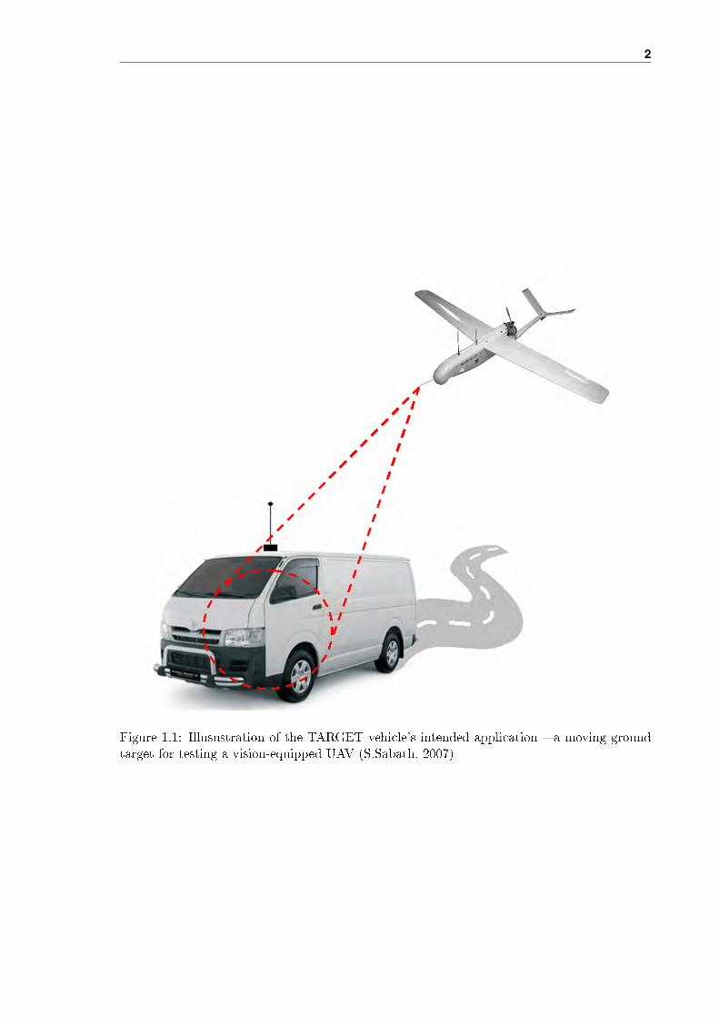
1.1 Illusustration of the TARGET vehicle's intended application a moving ground
target for testing a vision-equipped UAV (S.Sabath, 2007) . . . . . . . . . . . 2
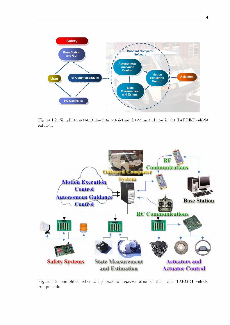
1.2 Simplied systems owchart depicting the command ow in the TARGET ve-
hicle solution . . . . . . . . . . . . . . . . . . . . . . . . . . . . . . . . . . . . 4
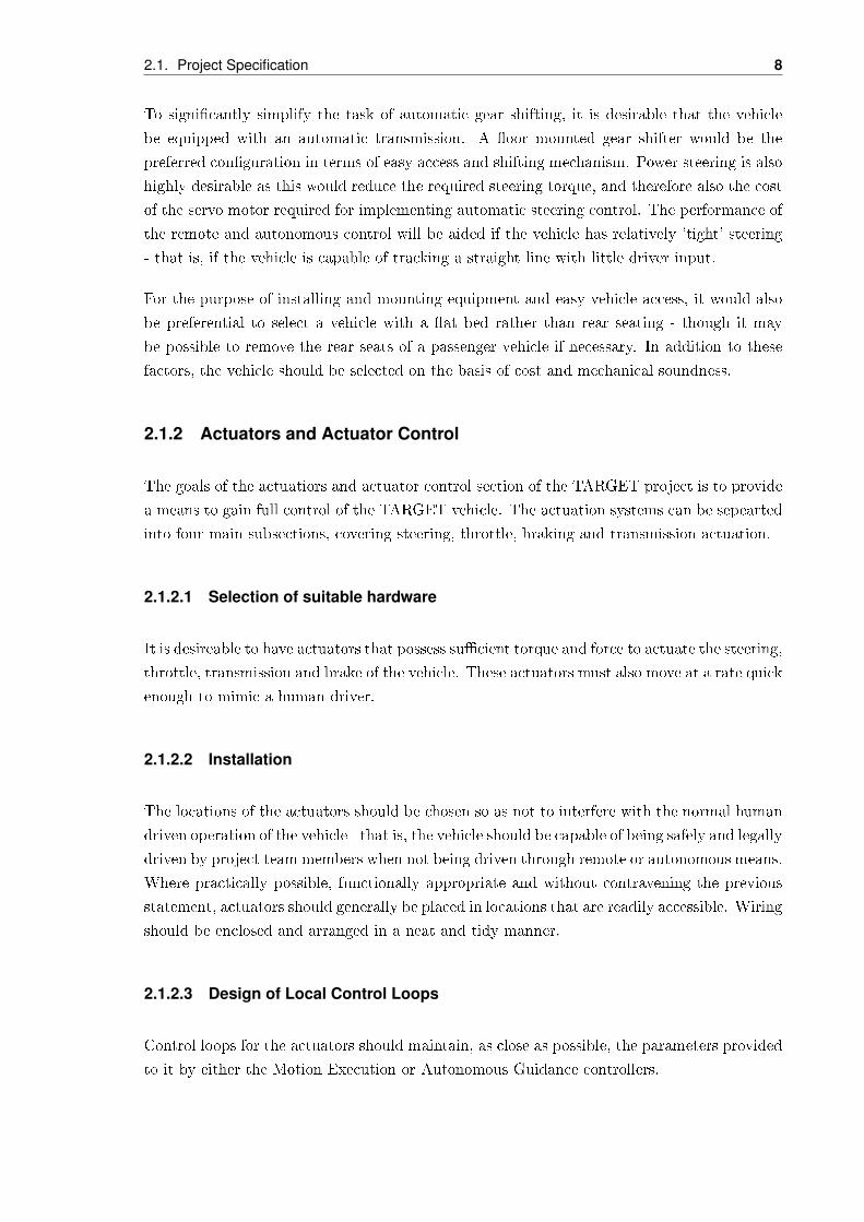
1.3 Simplied schematic / pictorial representation of the major TARGET vehicle
components . . . . . . . . . . . . . . . . . . . . . . . . . . . . . . . . . . . . . 4
3.1 Princeton University DARPA Grand Challenge vehicle (Atreya et al., 2005) . 20
3.2 Autonomous Vehicle Systems DARPA Grand Challenge vehicle (Vest, 2005) . 21
3.3 Steering actuation system (?) . . . . . . . . . . . . . . . . . . . . . . . . . . . 21
3.4 Brake actuation systems of Austin Robot Inc. (Brogdon et al., 2005) . . . . . 22
3.5 Possible arrangement connecting between the steel cable and the vehicle brake
pedal . . . . . . . . . . . . . . . . . . . . . . . . . . . . . . . . . . . . . . . . . 23
3.6 Possible mounting arrangement for the transmission actuation's linear actuator 24
3.7 The NAVSTAR GPS constellationGPS . . . . . . . . . . . . . . . . . . . . . . 25
3.8 The Novatel OEM4-G2 GPS processing card with accompanying Novatel GPS
AntennaTM Model 511 . . . . . . . . . . . . . . . . . . . . . . . . . . . . . . . 26
3.9 The Microstrain 3DM-GX1 IMU . . . . . . . . . . . . . . . . . . . . . . . . . 29
3.10 The gyroscope assemblyVerplaetse (1996) . . . . . . . . . . . . . . . . . . . . 30
3.11 The Honeywell GT1 Series 1GT101DC Solid State Hall-Eect Sensor(Honeywell) 31
3.12 The ETI Systems 10-Turn Wire-Wound 1 kΩ Rated Precision Potentiome-
ter(Systems, 2006) . . . . . . . . . . . . . . . . . . . . . . . . . . . . . . . . . 32
xxi

List of Figures xxii
3.13 The Earth-Centered Earth-Fixed Datum . . . . . . . . . . . . . . . . . . . . . 35
3.14 The Geodetic Datum . . . . . . . . . . . . . . . . . . . . . . . . . . . . . . . . 36
3.15 The Tangent Plane . . . . . . . . . . . . . . . . . . . . . . . . . . . . . . . . 37
3.16 Follow-the-carrot and pure pursuit path tracking control strategy (sourced from
Barton (2001)) . . . . . . . . . . . . . . . . . . . . . . . . . . . . . . . . . . . 40
3.17 Virtual Vehicle spatial guidance control strategy . . . . . . . . . . . . . . . . 41
3.18 Spatial guidance control parameters of cross-track error, d⊥, and heading error,
θe . . . . . . . . . . . . . . . . . . . . . . . . . . . . . . . . . . . . . . . . . . . 43
3.19 Simulated path following using a feedback controller (sourced from Barton (2001)) 44
3.20 Simulated path following using an additional feedforward term (sourced from
Barton (2001)) . . . . . . . . . . . . . . . . . . . . . . . . . . . . . . . . . . . 45
3.21 Tuned PID controller (Sourced from Qiu and Zhang (2003)) . . . . . . . . . . 46
3.22 Tuned FPID controller (Sourced from Qiu and Zhang (2003)) . . . . . . . . . 47
3.23 Throttle / brake switching logic as implemented (Sourced from Kwon et al.
(2001)) . . . . . . . . . . . . . . . . . . . . . . . . . . . . . . . . . . . . . . . . 48
3.24 PI throttle controller block diagram (Sourced from Kwon et al. (2001)) . . . . 49
3.25 PI throttle controller test results (Sourced from Kwon et al. (2001)) . . . . . . 49
3.26 PID plus feed forward performance characteristics (Sourced from Yi, et al. 2005) 50
3.27 Linear splines between waypoints (Lu, 2007) . . . . . . . . . . . . . . . . . . . 51
3.28 Inserting pseudo points to generate a path (Lu, 2007) . . . . . . . . . . . . . . 52
3.29 Natural cubic splines, identied as a suitable method of path generation . . . 52
3.30 The advantage of adding extra waypoints to construct a smooth and achieveable
path . . . . . . . . . . . . . . . . . . . . . . . . . . . . . . . . . . . . . . . . . 55
3.31 The rst, and easiest, method for dening a background image. Dene a ref-
erence point and specify the height and width of the image. The top of the
image is assumed to be north. . . . . . . . . . . . . . . . . . . . . . . . . . . . 55
3.32 The second, and more complicated method for dening a background image.
Place three points on the image. The location, orientation and skew can all be
dened by these points. . . . . . . . . . . . . . . . . . . . . . . . . . . . . . . 56
xxiii List of Figures
3.33 A typical handheld remote-control (RF Innovations Ltd Pty, 2007) . . . . . . 57
3.34 Caterpillar(TM) Trucks in open-pit mines (RF Innovations Ltd Pty, 2007) . . 59
3.35 An Automated Straddle control system by the Patrick Corporation (RF Inno-
vations Ltd Pty, 2007) . . . . . . . . . . . . . . . . . . . . . . . . . . . . . . . 59
4.1 The TARGET vehicle after being purchased and minor modications made . 65
4.2 Allocated frequency channels on the X2720 Remote-Control . . . . . . . . . . 69
4.3 The RFI-9256 RF Modem (RF Innovations Pty Ltd, 2006) . . . . . . . . . . . 70
4.4 Basic Hayes Dial-Up Network conguration (RF Innovations Pty Ltd, 2006) . 71
4.5 Data path operation of the RFI-9256 (RF Innovations Pty Ltd, 2006) . . . . . 71
4.6 Bisongear 348 Series PMDC Gearmotor (Bison Gear & Engineering Corp, 2007) 74
4.7 Steering column of TARGET vehicle . . . . . . . . . . . . . . . . . . . . . . . 75
4.8 TARGET Vehicle steering actuation system . . . . . . . . . . . . . . . . . . . 76
4.9 Steering potentiometer . . . . . . . . . . . . . . . . . . . . . . . . . . . . . . . 77
4.10 Instructions describing how to connect the actuator to the vehicle vacuum line
(Auscruise By Autron, 2007) . . . . . . . . . . . . . . . . . . . . . . . . . . . 78
4.11 TARGET throttle actuation system . . . . . . . . . . . . . . . . . . . . . . . . 79
4.12 A brief overview showing the sequential operation of the primary brake actua-
tion system . . . . . . . . . . . . . . . . . . . . . . . . . . . . . . . . . . . . . 80
4.13 Linear actuator's performance chart - Refer to 20:1 ratio for primary brake
actuation. This ratio represent the gear ratio embedded in the linear actuator.
(Firgelly Automation, 2007) . . . . . . . . . . . . . . . . . . . . . . . . . . . . 81
4.14 The TARGET vehicle's brake and transmission actuator assembly . . . . . . . 82
4.15 Pressure transducer GE Druck - PTX 1400 . . . . . . . . . . . . . . . . . . . 83
4.16 Modied circuit diagram of the pressure transducer to generate the desired
voltage output . . . . . . . . . . . . . . . . . . . . . . . . . . . . . . . . . . . 84
4.17 Mounting arrangement for the pressure transducer of the TARGET vehicle . . 84
4.18 Pictorial representations of individual components and the assembled compo-
nent for brake line modication purpose . . . . . . . . . . . . . . . . . . . . . 85

List of Figures xxiv
4.19 Detailed pictorial representation of the brake cable attachment . . . . . . . . 86
4.20 Brake pedal and brake cable link of the TARGET vehicle . . . . . . . . . . . 87
4.21 Emergency Brake System of the TARGET vehicle . . . . . . . . . . . . . . . . 88
4.22 Transmission actuation block diagram . . . . . . . . . . . . . . . . . . . . . . 89
4.23 Modied gear transmission lever of the TARGET vehicle. Mechanical lever
is indicated by the red circle in Subgure (a) and (b), modication to enable
linkage between the linear actuator and transmission lever is indicated by the
blue circle in Subgure (a) . . . . . . . . . . . . . . . . . . . . . . . . . . . . . 90
4.24 Linkage between transmission lever and actuator . . . . . . . . . . . . . . . . 90
4.25 Solenoid installation to the vehicle transmission lever. Highlighted in red-
coloured circle is the solenoid which connect the solenoid to the mechanical
lever . . . . . . . . . . . . . . . . . . . . . . . . . . . . . . . . . . . . . . . . . 91
4.26 Modied dash-board of the TARGET vehicle for gear position signal acquisi-
tions . . . . . . . . . . . . . . . . . . . . . . . . . . . . . . . . . . . . . . . . 93
4.27 Close-up view of the TARGET electronics. Highlighted in yellow circle is the
PCB board to accumulate gear position signal before connected to the TAR-
GET computer . . . . . . . . . . . . . . . . . . . . . . . . . . . . . . . . . . . 94
4.28 TARGET electronics . . . . . . . . . . . . . . . . . . . . . . . . . . . . . . . 95
4.29 Jaycar Electronics 1000 W pure sine wave inverter (Jaycar Electronics, 2007) 96
4.30 Capacitive Sensor . . . . . . . . . . . . . . . . . . . . . . . . . . . . . . . . . . 97
4.31 Roboteq AX1500 DC motor controller (Roboteq, 2007) . . . . . . . . . . . . . 100
5.1 The Extended Kalman Filter Algorithm . . . . . . . . . . . . . . . . . . . . . 105
5.2 A visual representation of the states to be determined . . . . . . . . . . . . . 106
5.3 GPS card (TBD) . . . . . . . . . . . . . . . . . . . . . . . . . . . . . . . . . . 112
5.4 GPS antenna (TBD) . . . . . . . . . . . . . . . . . . . . . . . . . . . . . . . . 113
5.5 The GPS data decoding program . . . . . . . . . . . . . . . . . . . . . . . . . 115
5.6 Subsystem to decode a four-byte single-precision oating-point number . . . . 117
5.7 Subsystem to decode an eight-byte double-precision oating-point number . . 118

xxv List of Figures
5.8 Subsystem to decode a four-byte long signed integer . . . . . . . . . . . . . . 118
5.9 Subsystem to decode a two-byte short unsigned integer . . . . . . . . . . . . . 118
5.10 ECEF to Geodetic datum conversion iteration . . . . . . . . . . . . . . . . . . 120
5.11 The datum transformation of the position standard deviation . . . . . . . . . 121
5.12 Vector visualisation of the longitudinal position standard deviation . . . . . . 122
5.13 Vector visualisation of the latitudinal position standard deviation . . . . . . . 123
5.14 Vector visualisation of the height position standard deviation . . . . . . . . . 123
5.15 The Northing . . . . . . . . . . . . . . . . . . . . . . . . . . . . . . . . . . . . 124
5.16 The Easting viewed looking down on the North Pole . . . . . . . . . . . . . . 124
5.17 The Easting viewed looking at the Earth from the side . . . . . . . . . . . . . 125
5.18 I need a caption...and a picture (TBD) . . . . . . . . . . . . . . . . . . . . . . 135
5.19 The IMU data decoding program . . . . . . . . . . . . . . . . . . . . . . . . . 136
5.20 Subsystem to decode a short signed integer . . . . . . . . . . . . . . . . . . . 137
5.21 Mounted hall eect sensor (TBD) . . . . . . . . . . . . . . . . . . . . . . . . . 141
5.22 Hall eect sensor setup (TBD) . . . . . . . . . . . . . . . . . . . . . . . . . . 142
6.1 Onboard computer program (top level) . . . . . . . . . . . . . . . . . . . . . . 148
6.2 I/O signals subsystem (top level) . . . . . . . . . . . . . . . . . . . . . . . . . 149
6.3 Steering potentiometer low-pass lter performance (TBD) . . . . . . . . . . . 151
6.4 Pressure transducer low-pass lter performance (TBD) . . . . . . . . . . . . . 151
6.5 Tachometer reading low-pass lter performance (TBD) . . . . . . . . . . . . . 152
6.6 Hall eect speed sensor low-pass lter performance (TBD) . . . . . . . . . . . 152
6.7 RC receiver channels 1 and 2 low-pass lter performance (TBD) . . . . . . . . 152
6.8 Fault detection subsystem top level . . . . . . . . . . . . . . . . . . . . . . . . 155
6.9 Mode chart top level . . . . . . . . . . . . . . . . . . . . . . . . . . . . . . . . 158
6.10 Normal Operation state top level . . . . . . . . . . . . . . . . . . . . . . . . . 160

List of Figures xxvi
6.11 Startup routine . . . . . . . . . . . . . . . . . . . . . . . . . . . . . . . . . . . 163
6.12 General autonomous control ow . . . . . . . . . . . . . . . . . . . . . . . . . 165
6.13 Autonomous control environment . . . . . . . . . . . . . . . . . . . . . . . . . 167
6.14 Speed guidance control scheme . . . . . . . . . . . . . . . . . . . . . . . . . . 170
6.15 Illustration of the importance of speed guidance control when operating on
bounded roads . . . . . . . . . . . . . . . . . . . . . . . . . . . . . . . . . . . 171
6.16 Autonomous controller structure . . . . . . . . . . . . . . . . . . . . . . . . . 171
6.17 Virtual vehicle search vectors . . . . . . . . . . . . . . . . . . . . . . . . . . . 173
6.18 Virtual vehicle point located behind current path segment . . . . . . . . . . . 173
6.19 Virtual vehicle point located beyond current path segment . . . . . . . . . . . 174
6.20 Vehicle located between path segments . . . . . . . . . . . . . . . . . . . . . . 175
6.21 Determining the orientation of the virtual vehicle path segment . . . . . . . . 176
6.22 Calculating the cross-track error, d⊥ . . . . . . . . . . . . . . . . . . . . . . . 176
6.23 Guidance Controller as implemented in Simulink . . . . . . . . . . . . . . . . 179
6.24 Autonomous control simulation model . . . . . . . . . . . . . . . . . . . . . . 181
6.25 Motion Execution Controller model . . . . . . . . . . . . . . . . . . . . . . . . 181
6.26 Unit step response of Motion Execution Controller model . . . . . . . . . . . 182
6.27 Simulink implementation of the Mathematical Vehicle Model . . . . . . . . . 183
6.28 Simulated open path-tracking performance of the Autonomous Guidance Con-
troller . . . . . . . . . . . . . . . . . . . . . . . . . . . . . . . . . . . . . . . . 185
6.29 Simulated closed-circuit path tracking performance of the Autonomous Guid-
ance Controller . . . . . . . . . . . . . . . . . . . . . . . . . . . . . . . . . . . 186
6.30 Steering Control System . . . . . . . . . . . . . . . . . . . . . . . . . . . . . . 188
6.31 Roll Prevention Saturation . . . . . . . . . . . . . . . . . . . . . . . . . . . . . 188
6.32 Roll Prevention Analysis 1 . . . . . . . . . . . . . . . . . . . . . . . . . . . . . 189
6.33 Roll Prevention Analysis 2 . . . . . . . . . . . . . . . . . . . . . . . . . . . . . 190
6.34 Steering Lock Saturation . . . . . . . . . . . . . . . . . . . . . . . . . . . . . . 191

xxvii List of Figures
6.35 Speed Control System . . . . . . . . . . . . . . . . . . . . . . . . . . . . . . . 192
6.36 Speed Switching Logic . . . . . . . . . . . . . . . . . . . . . . . . . . . . . . . 193
6.37 Closed Loop Throttle Controller . . . . . . . . . . . . . . . . . . . . . . . . . 194
6.38 Closed Loop Brake Controller . . . . . . . . . . . . . . . . . . . . . . . . . . 194
7.1 Various path types for the same ve waypoints. The vehicle is represented as
a blue dot. . . . . . . . . . . . . . . . . . . . . . . . . . . . . . . . . . . . . . . 197
7.2 Event sequence showing data inow, events and event recipients . . . . . . . . 198
7.3 Simplied ow diagram of the overall base station software. Blue represents an
internal manager, orange represents the visual objects on the monitor, yellow
represents data storage and green represents external objects. . . . . . . . . . 201
7.4 Screen shot of the current base station software . . . . . . . . . . . . . . . . . 202
8.1 Dragon Stop System . . . . . . . . . . . . . . . . . . . . . . . . . . . . . . . . 205
9.1 Steering step response (TBD) . . . . . . . . . . . . . . . . . . . . . . . . . . . 214
9.2 Braking step response (TBD) . . . . . . . . . . . . . . . . . . . . . . . . . . . 215
J.1 Screenshot of the base station software showing various dierent components
on the screen . . . . . . . . . . . . . . . . . . . . . . . . . . . . . . . . . . . . 271
J.2 The communication panel where the user can select the COM port and speed
of the serial connection . . . . . . . . . . . . . . . . . . . . . . . . . . . . . . . 272
J.3 The vehicle mode panel which is used to change the operating mode of the
TARGET vehicle . . . . . . . . . . . . . . . . . . . . . . . . . . . . . . . . . . 272
J.4 The zoom panel which provides tools for zooming the map area . . . . . . . . 273
J.5 The picture panel which allows graphs to be generated from the log le . . . . 274

List of Figures xxviii
List of Tables
3.1 Kalman Filter comparisons . . . . . . . . . . . . . . . . . . . . . . . . . . . . 34
3.2 Autonomous Guidance Control research criteria . . . . . . . . . . . . . . . . . 38
3.3 Comparison of PPM and PCM Systems for handheld remote-controls (Rother,
2007) . . . . . . . . . . . . . . . . . . . . . . . . . . . . . . . . . . . . . . . . 58
4.1 Comparison table between the required and actual performance of the linear
actuator . . . . . . . . . . . . . . . . . . . . . . . . . . . . . . . . . . . . . . . 82
4.2 Braking Conditions and the expected pressure range - Mitsubishi Express 1994 83
4.3 Specication for the electromagnet . . . . . . . . . . . . . . . . . . . . . . . . 88
4.4 Specication for the compressional spring . . . . . . . . . . . . . . . . . . . . 89
4.5 Comparison table between the expected performance of the linear actuator and
the selected specication of the actuator . . . . . . . . . . . . . . . . . . . . . 92
5.1 The header component of the BESTXYZB log . . . . . . . . . . . . . . . . . . 116
5.2 Format of the BESTXYZ log . . . . . . . . . . . . . . . . . . . . . . . . . . . 116
5.3 Transform errors . . . . . . . . . . . . . . . . . . . . . . . . . . . . . . . . . . 134
5.4 Response of the 3DM-GX1 to the 0x31 command . . . . . . . . . . . . . . . 136
6.1 Input and output signals list . . . . . . . . . . . . . . . . . . . . . . . . . . . . 150
6.2 Input signal scaling . . . . . . . . . . . . . . . . . . . . . . . . . . . . . . . . . 151
6.3 Faults monitored by onboard computer . . . . . . . . . . . . . . . . . . . . . . 155
6.4 Autonomous Guidance Control Performance Comparison . . . . . . . . . . . . 184
xxix

List of Tables xxx
7.1 A sample log le generated by the base station . . . . . . . . . . . . . . . . . 199
9.1 Steering controller step response characteristics . . . . . . . . . . . . . . . . . 214
9.2 Braking controller step response characteristics . . . . . . . . . . . . . . . . . 215
9.3 RF9256's Diagnostic and Statistics Results . . . . . . . . . . . . . . . . . . . . 220
K.1 Costing Parameters for labour hours . . . . . . . . . . . . . . . . . . . . . . . 275
K.2 Total manual labour hours (up to September 30th) and costs per team member 275
K.3 Total manual labour hours and costs per workshop . . . . . . . . . . . . . . . 276

Chapter 1
Introduction
This report describes the development, from concept to realisation, of a full-scale autonomous
ground target vehicle called the Thales Autonomous Radio-controlled Ground-basEd Tar-
get or its corresponding acronym, The TARGET. This challenging and innovative project
was carried out by a team of nine Undergraduate Mechatronic and Mechanical Engineering
students from The University of Adelaide in South Australia for the partial fullment of their
nal year Bachelor of Engineering study in 2007.
The TARGET vehicle at the centre of this undertaking is rst and foremost an unmanned
autonomous ground vehicle. The research eld of unmanned autonomous ground vehicles has
emerged as a growing area of technological pursuit and, despite its relatively young status,
such vehicles have already proved their signicant value in a surprisingly broad and expanding
range of applications in areas including defence, surveillance and security, mining, agriculture,
automotive transportation and space exploration. The utility of these vehicles essentially
arises from their potential to automatically and consistently follow a desired and recongurable
ground-based path to a high level of accuracy and without the need for a human driver. These
attributes advantageously predispose such vehicles to ground-based motion tasks which are
repetitive and monotonous, exposed to hazardous environments, and / or demand very precise
path tracking.
Through consultation with The University of Adelaide, the TARGET project was proposed
by Thales Australia, the Australian branch of a major international defence corporation, to
complement an Unmanned Aerial Vehicle (UAV) defence project that they were undertaking.
As illustrated in Figure 1.1, in order to test the tracking capabilities of their vision-equipped
UAV, Thales Australia required a tightly budgeted moving ground target vehicle. The po-
tential danger of the UAV colliding with the ground vehicle during testing created the need
for the moving ground target to be unmanned.
The TARGET project was therefore dened around the key objective of developing a safe
moving ground target vehicle system that was capable of switching between normal human
driving, remote control and autonomous control modes of operation. Such a vehicle would
1
2
Figure 1.1: Illusustration of the TARGET vehicle's intended application a moving groundtarget for testing a vision-equipped UAV (S.Sabath, 2007)

3 Chapter 1. Introduction
possess two modes of unmanned operation (remote control and autonomous control) in ad-
dition to the normal human-driven operation which would enable easy transportation to and
from testing grounds.
The implementation of autonomous obstacle avoidance strategies was deemed to be beyond the
scope of the project due to monetary and time constraints, and though it would have been
a welcome and desirable addition, it was not necessary for the achievement of the project
objectives or for the development of an eective autonomous ground target vehicle suited to
the specied application. With reference to the major project subsystems, Chapter 2 details
the general project scope and full assortment of project goals and specications that were
written into the project contract at the beginning of the project as a benchmark against
which to compare the nal project outcomes.
The TARGET vehicle developed in this project was therefore a unique solution to a very
specic problem, but nevertheless one that extended from the body of established knowledge
regarding autonomous ground vehicles.
The completed TARGET vehicle system comprises the core complementary elements of:
• Actuation,
• Radio Frequency (RF) Communications,
• State Measurement and Estimation,
• Onboard Computer Systems,
• Autonomous Guidance Control,
• Motion Execution Control,
• Base Station and Graphical User Interface (GUI), and
• Safety.
A basic overview of the implemented TARGET vehicle solution is illustrated in Figure 1.2 and 1.3.
With reference to Figures 1.2 and 1.3, the integrated vehicle system, built on a Mitsubishi
Express van, is equipped with an automated system of actuating the vehicle driving controls
(steering, throttle, brake, transmission, and ignition) without inhibiting its normal human-
driven operation. An embedded computer system onboard the vehicle interfaces with the ve-
hicle actuators and various sensors. This onboard computer also operates a software program
which, among many functions, facilitates Autonomous Guidance Control, Motion Execution
Control, State Measurement and Estimation, and an assortment of safety logic. In State
Measurement and Estimation, an Extended Kalman Filter fuses multiple sensor data into
improved estimates of the vehicle states (position, velocity, and heading). These estimates
are required for Autonomous Guidance Control, Motion Execution Control, and telemetry.
4
Figure 1.2: Simplied systems owchart depicting the command ow in the TARGET vehiclesolution
Figure 1.3: Simplied schematic / pictorial representation of the major TARGET vehiclecomponents

5 Chapter 1. Introduction
In Radio-Controlled (RC) mode, a remote user provides driving commands by operating a
handheld RC controller. These commands are wirelessly transmitted to the onboard com-
puter where they are executed by the Motion Execution Controller which controls the vehicle
actuators. In autonomous mode, an operator at a remote base station computer enters a
desired path into a graphical user interface. This path is converted into multiple waypoints
which are wirelessly transmitted to the onboard computer via a pair of RF modems. The
Autonomous Guidance Controller then determines the appropriate vehicle driving commands
required to achieve path tracking, and these commands are executed by the Motion Execution
Controller.
The TARGET vehicle solution also incorporates a broad range of safety features including
multiple emergency stop systems, a wide range of automated fault detection and response
mechanisms, and an audio-visual warning system.
The report addresses each of the major TARGET systems separately and in detail.
• Related works are discussed in Chapter 3 as a separate Literature Review which draws
upon various themes relating to the major functional categories used in the TARGET
project.
• Actuation design is discussed in Chapter 4 together with other hardware design aspects
such as vehicle selection, onboard computer components, and the RF communications
equipment.
• Chapter 5 is devoted to a detailed discussion of the State Measurement and Estima-
tion system, and the Onboard Computer software, Autonomous Guidance Control, and
Motion Execution Control systems have been presented together in Chapter 6 as com-
ponents of the unied TARGET control strategy.
• The Base Station and Graphical User Interface (GUI) and the TARGET Safety systems
have also been presented separately in Chapters 7 and 8 respectively.
• The results obtained from testing the integrated TARGET vehicle are presented in
Chapter 9, with specic analysis devoted to the performance of each major TARGET
system as well as a discussion of the overall eectiveness of vehicle's operation and mode
switching behaviour.
• The Conclusion (Chapter 5.7) summarises the report and presents the nal outcomes
and achievements of the TARGET project with reference to the contractual goals and
specications formulated at the beginning of the project. Some consideration is also
given to potential avenues for the projects expansion in future years.
• To facilitate (and indeed encourage) expansion of the TARGET project by nal year
Undergraduate Engineering students in future years, a project software CD has been
attached to Appendix L. This CD contains the complete Java code for the Base Sta-
tion GUI and the annotated Simulink / xPC Target block diagrams used to program

6
the vehicle's onboard computer. In addition, the TARGET's Safe Operating Proce-
dure is presented in Appendix E, and an outline of the various software-related issues
encountered during the project is provided in Appendix A.
Budget & costings / other Appendices?

Chapter 2
Project Goals and Specification
This section of the report deals with the specications of the nal vehicle and the measurable
goals to be reached by the conclusion of the project. A set of extension goals have also been
specied. These goals will not necessarily be implemented in the nal vehicle design however
they will be attempted, time permitting.
2.1 Project Specification
This is an outline of the project specications for each subgroup. It covers the specic tasks
which will need to be completed for each subgroup. Some groups have been split into phase
one and phase two sections. In this case, it roughly indicates which areas of the project should
be attempted rst (in phase one) and at a later stage (in phase two).
2.1.1 Vehicle Selection and Maintenance
To allow adequate targeting of the autonomous ground vehicle from the Thales UAV, the
projected area of the vehicle as 'seen' by the UAV vision systems and must be approximately
9 square metres and relatively rectangular in shape. As the projected area will be primarily
composed of the side of the vehicle, this specication implies height, length and shape require-
ments which most closely correspond to vans or people movers. The vehicle is intended to be
operated on sealed or well maintained unsealed surfaces, so rugged four wheel drive capacity
is nonessential. It is required that the vehicle be able to maintain speeds greater than 40
kilometres per hour and possess a minimum turning radius of 7.5 metres or less. The vehicle
should be free of unrelated insignia and signage and provide a protective environment for the
necessary electronic equipment that will be installed and carried onboard. The University
of Adelaide also requires that the vehicle be equipped with a suitable cargo barrier for the
protection of passengers, and be able to t within the allocated University parking bay.
7
2.1. Project Specification 8
To signicantly simplify the task of automatic gear shifting, it is desirable that the vehicle
be equipped with an automatic transmission. A oor mounted gear shifter would be the
preferred conguration in terms of easy access and shifting mechanism. Power steering is also
highly desirable as this would reduce the required steering torque, and therefore also the cost
of the servo motor required for implementing automatic steering control. The performance of
the remote and autonomous control will be aided if the vehicle has relatively 'tight' steering
- that is, if the vehicle is capable of tracking a straight line with little driver input.
For the purpose of installing and mounting equipment and easy vehicle access, it would also
be preferential to select a vehicle with a at bed rather than rear seating - though it may
be possible to remove the rear seats of a passenger vehicle if necessary. In addition to these
factors, the vehicle should be selected on the basis of cost and mechanical soundness.
2.1.2 Actuators and Actuator Control
The goals of the actuatiors and actuator control section of the TARGET project is to provide
a means to gain full control of the TARGET vehicle. The actuation systems can be sepearted
into four main subsections, covering steering, throttle, braking and transmission actuation.
2.1.2.1 Selection of suitable hardware
It is desireable to have actuators that possess sucient torque and force to actuate the steering,
throttle, transmission and brake of the vehicle. These actuators must also move at a rate quick
enough to mimic a human driver.
2.1.2.2 Installation
The locations of the actuators should be chosen so as not to interfere with the normal human
driven operation of the vehicle - that is, the vehicle should be capable of being safely and legally
driven by project team members when not being driven through remote or autonomous means.
Where practically possible, functionally appropriate and without contravening the previous
statement, actuators should generally be placed in locations that are readily accessible. Wiring
should be enclosed and arranged in a neat and tidy manner.
2.1.2.3 Design of Local Control Loops
Control loops for the actuators should maintain, as close as possible, the parameters provided
to it by either the Motion Execution or Autonomous Guidance controllers.

9 Chapter 2. Project Goals and Specification
2.1.2.4 Safety
A reliable, failsafe mechanism for manually overriding the actuators will be developed to
enable a person in the driving seat to either immediately and easily stop or regain manual
control of the vehicle at any time.
2.1.3 Phase One Communication
2.1.3.1 Selection of a Suitable Communication System
The Phase One activity is concerned with establishing a 'drive-by-wire' system to provide
the capacity to maneuver the target vehicle using a human operated remote control. This
task will require a hand operated, short range, multichannel radio control (RC) transmitter
to translate remote human inputs of vehicle control commands (heading and speed) to a
corresponding onboard receiver over a one way radio frequency (RF) communication system.
PWM decoders will be used to enable the onboard processor (necessary for control) to read
the incoming commands.
2.1.3.2 Installation and Commissioning of Hardware
The RF receiver of the command signals transmitted by the short range, handheld radio
controller will be installed onboard the vehicle and connected to the onboard processor. Its
antenna will be positioned on the vehicle in such a way as to obtain adequate reception of the
RC signal.
2.1.4 Phase Two Communication
2.1.4.1 Selection of a Suitable Communication System
The Phase Two communication system will support two way communication between the
vehicle's onboard processor and the remote base station computer allowing waypoint position
commands to be sent to the vehicle and vehicle status information to be received by the
remote base station for visual display and monitoring. High speed data transfers over an
approximate range of ten kilometres and at an adequate bandwidth would be desirable for
this purpose.
2.1.4.2 Selection of Capable Hardware
Phase Two communication will require the selection of a suitable RF transceiver and antenna
to be installed both at the remote base station and onboard the vehicle. A wide bandwidth
is desired to support high speed data transfer.

2.1. Project Specification 10
2.1.4.3 Installation and Commissioning of Hardware
The base station RF transceiver will be connected to the base station computer and an RF
antenna. This arrangement should be portable as the vehicle will be tested in a number of
locations. The other RF transceiver will be installed on the vehicle and connected to the
onboard processor. The onboard RF transceiver will be securely mounted on the vehicle
in such a way as to minimise interference with the GPS signal (accurate autonomous control
relies on a relatively uncorrupted GPS signal), whilst also obtaining adequate reception. When
placing all antennas, care should be taken to ensure that the vehicle maintains an adequate
height clearance to enable travel on standard underpasses and in undercover car parks.
2.1.5 Motion Execution Control
2.1.5.1 Vehicle Steering and Speed Control
The desired vehicle steering and speed are to be transmitted to the onboard processor from the
handheld, human operated radio control via the one way communication link as inputs to the
Motion Execution Control system. When operating in autonomous mode, the desired vehicle
steering and speed will be generated by the Autonomous Guidance Control system and passed
on to the Motion Execution Controller. Closed loop feedback of the 'actual' vehicle steering
and speed will be provided by a Kalman Filter / estimator via a fusion of measurements from
the GPS, IMU, and other available vehicle sensors. The Motion Execution Control system
will then regulate output commands to the throttle, steering and brake actuators and ensure
that the vehicle responsively tracks the desired steering and speed.
2.1.5.2 Gearbox and Ignition Control
The Motion Execution Control system should also produce and handle control commands to
the vehicle ignition and gearbox, though local control loops embedded in the gearbox and
ignition actuator systems should be used to implement the actual automatic operation of
these devices.
2.1.5.3 Safe Operation
The controller must include appropriate safety logic to ensure safe operation of the vehicle,
though the vehicle should only be operated in an environment where the hazards posed to
human safety are minimal. The safety logic should include the ability to reliably override
autonomous control with radio / remote control at any time, an emergency stop mechanism,
logic to halt the vehicle during a loss of radio communications, and a roll prevention scheme.
It is also desirable for audio and visual warnings to be activated upon critical systems failure.

11 Chapter 2. Project Goals and Specification
2.1.5.4 Selection, Installation and Maintenance of the Vehicle’s Onboard Processor
The vehicle's onboard processor will interface with many of the vehicle systems. It will however
be under the most load while processing the engagement of vehicle control, state estimation,
and communication. The onboard processor platform should have sucient memory and
ops (oating point operations per second) to handle these tasks, and should be equipped
with enough peripherals and I/O ports to allow the seamless integration and interconnection of
the necessary devices. The processor platform should be able to operate under the vibration,
temperature, and other environmental conditions inside the vehicle. It should therefore be
enclosed in a suitable housing and securely mounted in a protected location within the vehicle.
For the purposes of systems integration, servicing, and maintenance, it is also desirable for
the processor platform to have a modular design and be easily accessible.
2.1.6 Autonomous Guidance Control
2.1.6.1 Waypoint Based Navigation and Guidance Control
The aim of the Autonomous Guidance Controller is to achieve safe and robust autonomous
closed loop vehicle navigation and guidance control based on a path delineated by a set of
position waypoints commands which are to be issued to the vehicle through the remote base
station computer. From a 'black box' perspective, the Autonomous Guidance Control system
should accept the position waypoint commands from the remote base station together with
a full feedback of actual vehicle state information (position, speed and heading) as obtained
by the fusion of GPS, IMU and other vehicle sensory measurements in a Kalman Filter /
estimator, and as an output provide the Motion Execution Control system with the speed
and heading commands required to implement the desired motion. The intelligent internal
workings of this system should achieve a smooth and suciently rapid vehicle motion with
reasonably accurate conformity to the commanded waypoint locations. Vehicle speed should
be regulated to ensure the stability of the vehicle at all times. The design of this control system
will require the development of a mathematical model of the relevant vehicle dynamics.
2.1.6.2 Acceptance of Waypoint Commands
It is desirable for the vehicle navigation and guidance control system to be capable of accepting
waypoint commands from the remote base station in two modes: as a pre-programmed batch
of waypoints describing a xed course, or as waypoints entered 'on the y' describing a
dynamically changing path. In both cases, the vehicle should stop after the nal specied
waypoint has been reached.

2.1. Project Specification 12
2.1.6.3 Performance Criteria
The Autonomous Guidance Control system should provide accurate vehicle navigation at
a minimum ordinary operating speed of 40 kilometres per hour. Under normal autonomous
operation, it is desirable (though dependent on the performance characteristics of the available
hardware - particularly the GPS unit) that the vehicle not deviate from the desired path
by more than 2 metres, so as to allow the vehicle the capacity to maintain a road bound
course without exceeding its outer boundaries. The vehicle should also possess a minimum
autonomous turning radius of 7.5 metres or less and be capable of continuous autonomous
navigation over a distance of 1.125 kilometres or greater.
2.1.6.4 Logic to Handle Loss of Communications
In the event of a critical sensor failure (that is, a failure of either the GPS or IMU) or an
unexpected loss of communications with the remote base station, the vehicle must immediately
and reliably decelerate to a stop or until normal communications or sensor function is restored.
2.1.6.5 Feedback of Data Back to Ground Station
The measured vehicle state information and controller commands should be transmitted to
the remote base station for inclusion in a vehicle status display.
2.1.6.6 Hardware Selection and Systems Integration
The Autonomous Guidance Control system will need to be integrated with the Kalman Filter
/ estimator and the Motion Execution Control system, and be programmed into the vehicle's
onboard processor platform. The task of selecting this platform has been described above,
and will depend on the requirements of a variety of tasks.
2.1.7 State Measurement and Estimation
2.1.7.1 Hardware Selection and Installation
The state measurement and estimation task will require the selection of a suitable GPS, IMU
and any additional vehicle sensors. Both the GPS and IMU should be mounted inside the
vehicle and preferably located along its cent reline. All sensors (including the GPS and IMU)
will need to be connected to the onboard processor so that their measurements can be used
as inputs to the vehicle state estimator / Kalman Filter. A capable GPS antenna will also
have to be selected and this should be located to allow the unobstructed reception of the GPS
satellite signals. As previously mentioned, the GPS antenna should also be kept isolated from
the onboard RF transceiver antenna in order to avoid interference.
13 Chapter 2. Project Goals and Specification
2.1.7.2 State Estimator / Kalman Filter Design
A mathematical model of the sensors (describing information such as time delays and satura-
tion points) will be required to implement this stage. The knowledge of the sensor mathematics
will be used as a basis for the selection of an accurate and practically viable method of state
estimation (most likely a form of Kalman Filter). This state estimator should be able to fuse
the available sensor measurements into a single, more accurate set of 'actual' vehicle state
estimates including vehicle position, heading and velocity.
2.1.7.3 Systems Integration
The state estimator / Kalman Filter should be integrated with the Motion Execution and
Autonomous Guidance control systems (which are dependent on the state estimates for closed
loop operation) and programmed into the vehicle's onboard processor platform.
2.1.8 HMI and GUI
2.1.8.1 Two Way Communication with the Onboard Processor
Commands to all actuators should be tested, although the vehicle will not be running at this
early stage. Known data will be sent from the vehicle's onboard processor to the basestation
computer and the accuracy then veried. The accuracy of the data sent from the basestation
to the onboard processor will also be tested.
2.1.8.2 Creation of a Simplified User Interface
This interface should simply require the user to provide a list of GPS waypoints, at the
basestation computer, which will then be transmitted to the vehicle. Vehicle information
(including speed, heading and position) should also be fed back and displayed at the base
station.
2.1.8.3 Upgrade to a Graphical User Interface (GUI)
The GUI should consist of a graphical representation of the path to be taken by the vehicle (i.e.
a map displaying all waypoints). The position of the vehicle on this map should be displayed at
the highest attainable refresh rate (depending on the hardware available) using the information
relayed back from the vehicle. The remaining vehicle states should be displayed on the GUI.
2.2. Project Goals 14
2.1.8.4 Hardware Selection
This task requires the selection of a suitable base station computer (preferably a laptop) and
associated peripherals. The remote base station needs to be portable in order for the vehicle
to be tested in dierent locations. It is also unlikely that mains power will be available so the
selection of an appropriate power supply (such as a generator or a battery and inverter) will
also be necessary.
2.1.9 Provision of Power
All of the vehicle power requirements are to be tabulated and this information should be
used as the basis for selecting appropriate batteries, ampliers and inverters as necessary.
The steering servo motor will most likely consume the largest amount of power due to the
large torque required to physically steer the vehicle (particularly at low speeds). The power
ampliers and all other low current hardware should share a separate power supply.
2.1.9.1 General Hardware/Software Selection
At least three quotes should be obtained for every item that is to be purchased. Where
possible, it is advantageous to select equipment that is familiar to Thales Australia or the
University of Adelaide. All hardware and software should generally be selected on the basis
of performance (including accuracy and response time), cost, reliability, compatibility and
modularity, availability, power consumption, and size and weight.
2.2 Project Goals
Select a suitable vehicle platform
The suitability of the chosen vehicle platform will be evaluated against the criteria described
in Section 2.1.1.
Select a suitable onboard vehicle processor
The suitability of the chosen onboard vehicle processor will be evaluated against the criteria
described in Section 9.3.6 of the Project Specication.

15 Chapter 2. Project Goals and Specification
Establish an effective automated system of actuating the vehicle driving controlswithout interfering with the normal human driven operation of the vehicle
The performance of the actuation system will be veried in pre-installation testing, as well
as post-installation commissioning testing, and testing under remote controlled vehicle op-
eration. Functionality, response time, command following, and reliability will be important
benchmarks. The capacity for safe and unimpeded normal human driven vehicle operation
post-installation will also be assessed and veried as satisfactory.
Establish an effective short range oneway RF communication link between a hand-held radio control transmitter and the vehicle’s onboard processor
Progress in regards to establishing a short range one way RF communication link will be
measured via small scale laboratory tests that will verify when the performance required for
successful data transfers from the human operated handheld remote control to the target
vehicle is achieved. These Phase One tests will use a simplied version of the full scale
system to independently test the handheld remote control's operability factors such as range,
speed, stability, precision benchmarks (yet to be determined), and reliability. A Cathode Ray
Oscilloscope (CRO) will be used to analyse output signals and ensure that the PWM decoder
is capable of sending acceptable signals to operate parts of the vehicle such as the servo
motors. Testing will take place strategically at various stages throughout the construction of
the target vehicle.
Establish an effective two way RF communication link between the remote base sta-tion computer and the vehicle’s onboard processor
Progress in regards to establishing the two way RF communication link will be measured via
small scaled laboratory tests that will verify when the performance required for successful data
transfers between the target vehicle and the base station is achieved. These Phase Two tests
will use a simplied version of the full scale system to independently test the RF modems'
operability factors such as range (ten kilometres), speed, stability, precision, benchmarks (yet
to be determined), and data reliability. Desktop PCs will be used in the early testing stages to
replace the actual processors used in the full scale system. Temporary code running in Matlab
or Simulink (on a real time target) or C will be used to assess maximum data transfers and
highlight any potential for data dropouts or loss of communications. Further testing will take
place strategically at various stages throughout the construction of the target vehicle.
Derive an accurate mathematical model of the relevant vehicle dynamics
The accuracy of the vehicle control systems will rely to an extent on the accuracy of the math-
ematical modeling of the vehicle dynamics. It will be essential for the vehicle steering to be

2.2. Project Goals 16
modeled, and if time permits a model (either linear or nonlinear) of the vehicle's acceleration
and braking dynamics will also be incorporated. The accuracy of the mathematical model
can be ascertained by comparing the simulated vehicle behavior against the actual vehicle
behavior when both are exposed to the same stimuli.
Enable the effective fusion of all available sensor measurements into a single, moreaccurate set of ’actual’ vehicle states using a Kalman Filter / state estimator
Sensor fusion performance will be established from a comparison between raw sensor measure-
ments of vehicle states and fused measurements of vehicle states including vehicle position,
heading and velocity. This will involve logging the data entering the vehicle processor from
all sensors. The output states of the estimator will also be logged. A comparison will then
be made between the values of the estimated states and the raw sensor data, over time. The
performance of the estimator will be determined according to the continuity of the state data
and its derivatives (e.g. the position of the vehicle as sensed by the GPS unit may jump by
several meters within a split second, however the estimated position of the vehicle should not
do so).
Achieve successful remote controlled operation of the target vehicle
All of the predescribed safety mechanisms will be tested and their eective and consistent
dependability ensured before operating the vehicle by remote or autonomous means. The
performance of the remote control vehicle operation will be assessed in a number of trials.
The underlying Motion Execution Control system will also rst be tested in simulation before
being implemented in practice. Important criteria will include operability, responsiveness,
stability and reliability, and command following.
Provide a graphical user interface (GUI) for the visual display and monitoring of ve-hicle status at a portable remote base station, and allow the commanding of positionwaypoints both ’onthefly’ and as a preprogrammed batch
The graphical user interface (GUI) will be evaluated on the basis of functionality, utility,
ergonomics and reliability. The issuing and tracking of waypoint commands in both the
'onthey' and preprogrammed modes will be examined in separate tests during autonomous
vehicle operation.
Achieve successful autonomous control of the target vehicle
The autonomous vehicle navigation and guidance will be assessed against the performance
criteria described in Section 2.1.6. Before operating the vehicle in autonomous mode, the
17 Chapter 2. Project Goals and Specification
failsafe safety mechanisms must be ensured, and the navigation and control system will be
rst tested in simulation. The autonomous system should be shown to achieve a smooth
and suciently rapid intelligent vehicle motion with reasonably accurate conformity to the
commanded waypoint locations.
Enable intelligent and safe switching between normal human driving, remote controland autonomous modes of operation
The seamless switching of vehicle control between a human driver, the remote controller, and
the remote base station (in autonomous mode) will be veried in trials.
2.3 Extension Goals
The extension goals listed below are not specied as being required for the completed vehicle.
They are intended to be extra goals that should be met if possible, working around time and
budget constraints.
• Investigate the possibility of making the vehicle street legal for normal human driving.
• Enable teleoperation of the vehicle using a handheld controller connected to the remote
base station computer.
• Attach an onboard camera to stream video footage to the base station GUI.
• Develop a virtual reality model of the autonomous vehicle as a whole.
• Incorporate additional controlled states (such as pitch, roll or turn rate) to further
enhance and expand the dynamic vehicle control.
• Develop and test dierent and / or more advanced control strategies.
• Develop and test dierent and / or more advanced methods of state estimation.

2.3. Extension Goals 18
Chapter 3
Literature Review
A literature review was conducted to investigate the various ways in which other teams and
researchers have tackled the challenge of designing the dierent systems comprising an au-
tonomous vehicle. A number of dierent sources were investigated including the internet,
journal articles and books. The information gained during this research period helped to pro-
vide a starting point upon which the designs of the various systems of the TARGET vehicle
could be based.
The literature review was concentrated on 6 dierent areas of research and these will be
discussed further in this chapter:
1. Vehicle actuation systems
2. Motion execution control systems
3. Autonomous guidance control systems
4. State measurement and estimation
5. Vehicle path generation and imaging
6. Radio communications
3.1 Steering
Steering actuation, being the automated control of the steering of a motor vehicle, is a pivotal
element of the TARGET project. Although there is a paucity of relevant literature regarding
steering actuation, the current Literature Review aims to identify the strengths and weak-
nesses in the existing approaches in order to provide a rm basis for the development of a
steering actuation system in the TARGET project. As steering actuation is seldom utilized
19

3.1. Steering 20
in modern motor vehicles, the vast majority of the concerned literature is based upon vehicles
that participated in the DARPA Grand Challenge.
Analysis of steering systems found in reports from teams that participated in the DARPA
Grand Challenge found that there was no commonly adopted approach to actuate the steering
of an autonomous vehicle. However, there were common elements in many of the steering
actuation systems of vehicles of a similar age and layout to the vehicle platform being used
in the TARGET project. These common elements were to use an electric motor to provide a
driving force and couple this to the steering column using a linkage system.
A steering actuation system developed by the Princeton University DARPA challenge team
is shown in Figure 3.1. This steering system consists of a motor which is coupled with the
steering column by a series of gears. Bodywork surrounding the steering column behind the
steering wheel has been removed in order to expose sections of the steering column to attach
the gears. The motor is placed below and parallel to the steering column (Atreya et al., 2005).
Figure 3.1: Princeton University DARPA Grand Challenge vehicle (Atreya et al., 2005)
Similar to the team from Princeton University, the Autonomous Vehicle Systems DARPA
Grand Challenge team (Figure 3.2) actuated the steering behind the steering wheel. However,
the Autonomous Vehicle Systems team utilized a toothed belt and pulley arrangement, by
tting pulleys around the steering column and DC motor shaft, and running the belt around
these two pulleys. The use of a toothed belt by the Autonomous Vehicle Systems Team
eliminated the risk of the belt slipping from its desired location (Vest, 2005).
Figure 3.3 shows a DC motor, in which the output shaft of the motor is perpendicular to the
output shaft of the gear head. This allows the motor to be mounted in the position shown,
as opposed to the parallel mountings illustrated in Figures 3.1 and 3.2. In this example, the
output shaft of the motor is coupled to the steering column with a chain and sprockets to
provide steering actuation. The position of the motor only interferes with the foot rest to
the left of the brake pedal, and does not interfere with any manual use of the pedals of the
vehicle. Therefore, the vehicle can still be operated both manually and autonomously.

21 Chapter 3. Literature Review
Figure 3.2: Autonomous Vehicle Systems DARPA Grand Challenge vehicle (Vest, 2005)
Figure 3.3: Steering actuation system (?)
3.2 Brake Actuation
The main objective of the brake actuation system was to enable vehicle deceleration during
autonomous and emergency operation modes. Furthermore, the modication performed to
the selected vehicle must not interfere with the normal operation of the vehicle.

3.2. Brake Actuation 22
(a) Electromagnet dis-energized - emergency situation
(b) Electromagnet energized - autonomous operation
Figure 3.4: Brake actuation systems of Austin Robot Inc. (Brogdon et al., 2005)
The brake actuation system of the Austin Robot Inc. (a contestant for the DARPA Grand
Challenge) is achieved by two dierent means: the force produced by a linear actuator and
the force produced by a tensional spring. The linear actuator is used to actuate the vehicle
braking system during autonomous operation. On the other hand, the force produced by the
tensional spring is used to activate the vehicle braking system during emergency situations.
The installation set-up for the Austin Robot Inc. brake actuation system is shown in Figure
3.4. With reference to Figure 3.4, the electromagnet will be used to provide a holding force to
the tensional spring thus de-activating the emergency brake during autonomous and normal
human operation.
There are three main advantages associated with this type of actuation. Firstly, the possibility
to locate the linear actuator at a distance from the vehicle brake pedal. Secondly, enabling the
on-board driver to manually override the system at anytime with no interference. A highly
reliable emergency systems is the third main advantage because the secondary braking system
does not require any electrical power to be activated.
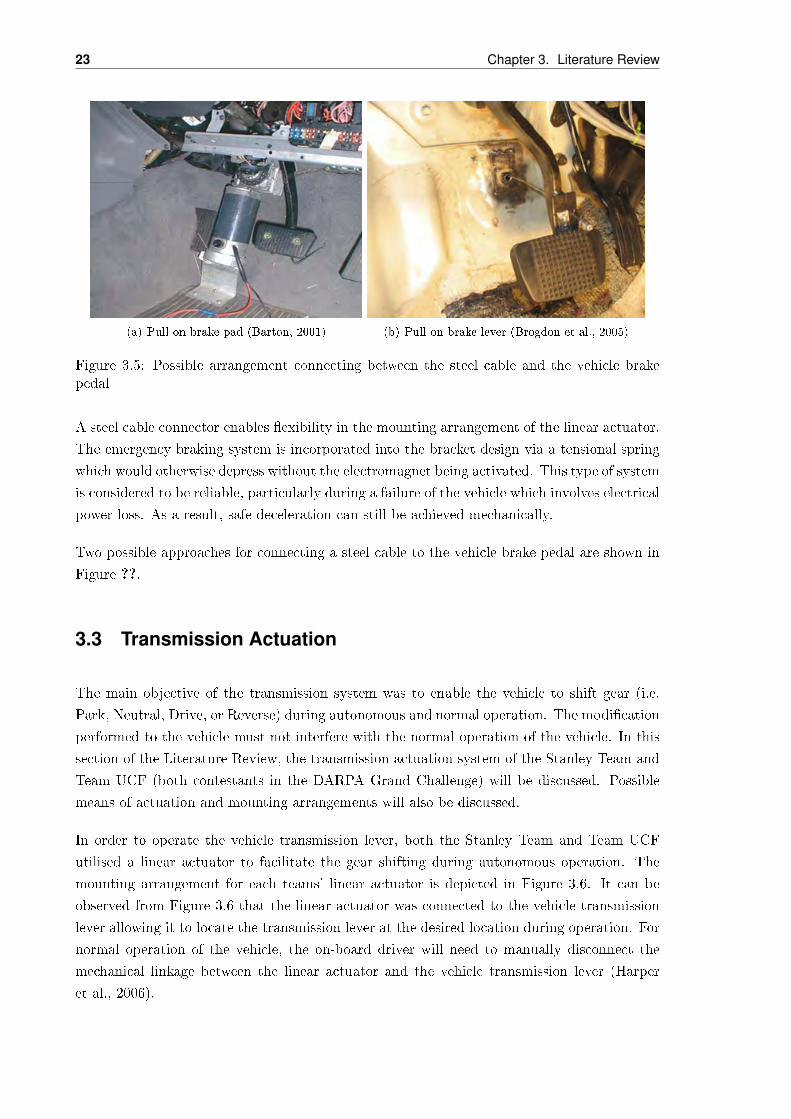
23 Chapter 3. Literature Review
(a) Pull on brake pad (Barton, 2001) (b) Pull on brake lever (Brogdon et al., 2005)
Figure 3.5: Possible arrangement connecting between the steel cable and the vehicle brakepedal
A steel cable connector enables exibility in the mounting arrangement of the linear actuator.
The emergency braking system is incorporated into the bracket design via a tensional spring
which would otherwise depress without the electromagnet being activated. This type of system
is considered to be reliable, particularly during a failure of the vehicle which involves electrical
power loss. As a result, safe deceleration can still be achieved mechanically.
Two possible approaches for connecting a steel cable to the vehicle brake pedal are shown in
Figure ??.
3.3 Transmission Actuation
The main objective of the transmission system was to enable the vehicle to shift gear (i.e.
Park, Neutral, Drive, or Reverse) during autonomous and normal operation. The modication
performed to the vehicle must not interfere with the normal operation of the vehicle. In this
section of the Literature Review, the transmission actuation system of the Stanley Team and
Team UCF (both contestants in the DARPA Grand Challenge) will be discussed. Possible
means of actuation and mounting arrangements will also be discussed.
In order to operate the vehicle transmission lever, both the Stanley Team and Team UCF
utilised a linear actuator to facilitate the gear shifting during autonomous operation. The
mounting arrangement for each teams' linear actuator is depicted in Figure 3.6. It can be
observed from Figure 3.6 that the linear actuator was connected to the vehicle transmission
lever allowing it to locate the transmission lever at the desired location during operation. For
normal operation of the vehicle, the on-board driver will need to manually disconnect the
mechanical linkage between the linear actuator and the vehicle transmission lever (Harper
et al., 2006).

3.4. State Estimation and Measurement 24
(a) Stanley's transmission system (Thrun et al., 2005) (b) Team UCF transmission system (Harper et al.,2005)
Figure 3.6: Possible mounting arrangement for the transmission actuation's linear actuator
3.4 State Estimation and Measurement
The process of State Estimation and Measurement, in relation to this project, involves the
real-time manipulation and improvement of data from a number of dierent vehicle sensors.
The result of this process is a set of vehicle states (or variables), which may be used to perform
automatic control of the vehicle motion and track a path. The aim of this literature review
section is to provide some of the background theory behind the practical processes presented in
the State Estimation and Measurement body section (Section ??). Firstly a breif description
of each of the sensors used in the State Estimation and Measurement process is given, followed
by a discussion of the advantages and dissadvantages of the main Kalman Filters currently
in existence; naly the three Earth coordinate systems utilised in the State Estimation and
Measurement body section are dened.
3.4.1 Sensor Functionality
The four sensors used in the State Estimation and Measurement process of the TARGET
vehicle are the Novatel OEM4-G2 Global Positioning System (GPS) processing card with
accompanying Novatel GPS AntennaTM Model 511 ; the Microstrain 3DM-GX1 Innertial
Measurement Unit ; the Honeywell GT1 Series 1GT101DC Solid State Hall-Eect Sensor
and the ETI Systems 10-Turn Wire-Wound 1 kΩ Rated Precision Potentiometer. A breif
description of the functional mechanism which governs each of these sensors, and the errors
which are likely to be encountered during their operation in the TARGET vehicle follows.
The GPS Unit
GPS units receive and process data from the GPS satelite constelation and output their own
position in space. The Navigation Satelite Timing and Ranging Global Positioning System
(NAVSTAR GPS) constelation comprises 24 satelites which orbit in 6 planes about the Earth
as shown in Figure3.7.

25 Chapter 3. Literature Review
Figure 3.7: The NAVSTAR GPS constellationGPS

3.4. State Estimation and Measurement 26
Figure 3.8: The Novatel OEM4-G2 GPS processing card with accompanying Novatel GPSAntennaTM Model 511
Each of these satelites transmitts a Navigation Message, consisting of ephemeris data, a pseu-
dorandom noise sequence and a variety of other data which is not relevant to this discussion.
The ephemeris data describes the current position of the transmitting satelite in its Keplarian
orbit and the pseudorandom noise sequence is used to determine the time of travel of the GPS
signal from the satelite to the receiver. These time dierences and the ephemeris data provide
sucient information for the receiver to trilaterate its own position in space of Defence (1995).
The main causes of GPS position errors are now listed and the correction method used by
the Novatel OEM4-G2, shown in Figure 3.8, is also described.
Atmospheric Delays The periodically varying density of the atmosphere causes the GPS
signal to slow down as it passes from the transmitting satelite to the GPS receiver unit.
Unaccounted for, atmospheric delays may cause position errors which vary from zero to forty
meters over the course of a year. However, an accurate model of the Earth's atmosphere
currently exists and may be used to drasticly reduce this error gure Herrington (1995). The
OEM4 family user manuals do not mention atmospheric delay corrections, however, since
the atmosphere model is well doumented, and since the typical position error range of the
OEM4 unit is stated to be in the order of two meters, it is assumed that the OEM4-G2 unit
encorporates the model into its position solution to correct for the majority of atmospheric
delays.
Ephemeris Errors Ephemeris errors occur when a satelite transmitts its own position er-
roneously Kelly (1994b). Since the receiver uses the satelite positions to determining its own
position, ephemeris errors result in a GPS receiver position error. This error is well described
by zero-mean, Gaussian noise with a standard deviation of the order of 0.5 meters Herrington
(1995). The OEM4-G2 has no means of correcting against ephemeris errors.

27 Chapter 3. Literature Review
Multipath Multipath errors occur when the signal transmitted from a GPS satelite bounces
o an object prior to reaching the receiver. This new transmission path incurs a time delay
which results in a position miscalculation by the receiver. To combat this unwanted phe-
nomenon, GPS signals are broadcast at frequencies of 1575.42MHz and 1227.6MHz (known
as the L1 and L2 bands) which tend to undergo diuse reection (i.e. the reection is dis-
persed), Herrington (1995), thus reducing the likelihood that the receiver will pick up a
multipath signal. In addition, the majority of multipath signals encountered in open areas
(such as the test grounds for the TARGET vehicle) approah the receiver antenna at an ele-
vation angle close to, or below, the horizontal. The Novatel GPS AntennaTM Model 511 has
the capacity to mask satelite signals below a user-dened elevation angle NovAtel Inc (2003),
p94, thereby eliminating the majority of multipath signals.
Receiver Noise Receiver noise is a product of quantisation and hardware inacuracies within
the GPS receiver Herrington (1995). The OEM4-G2 estimats the level of noise (especially
thermal noise) existent within its own hardware, and uses this gure to compute the standard
deviation of the position solution NovAtel Inc (2003), p198.
Dilution of Precision Dilution of precision (or DOP) of the GPS position solution occurs
when a signicant number of the satelites visble to the receiver antenna are closly spaced
Herrington (1995), p119. The eect of DOP is to amplify the other position solution errors,
at most by a factor of three. The OEM4-G2 recalculates the DOP status from ephemeris data
every 60 seconds and uses the resulting value to update its estimate of the standard deviation
of the position solution NovAtel Inc (2003), p193.
Signal Masking Signal masking, also known as signal dropout, occures when objects block
or distort the transmitted signals from a signicant number of GPS satelites, such that the
position solution becomes unavaliable Caron et al. (2006). Typical objects which are likely to
cause signal masking for the GPS receiver on the TARGET vehicle are trees, tall buildings,
power lines and the Earth itself. The Global Positioning System alone oeres no remedy
for signal masking, however other sensors may be used to provide position data during pe-
riods of GPS unavalibility. This technique forms a major part of the State Estimation and
Measurement process covered in this report.
The combined eect of the above errors on the OEM4-G2 receiver is a GPS position solution
with superimposed zero-mean Gaussian noise (due to the atmospheric delays, ephemeris data
and receiver noise), occasional position jumps (due to multipath eects) and ocasional total
position loss (due to signal masking). The position (containing multipath errors) and the
standard deviation of the Gaussian noise component of this signal are output by the OEM4-
G2.

3.4. State Estimation and Measurement 28
The IMU Sensor
The technology used in Inertial Measurement Units (IMUs) varies greatly accross the market,
with dierent brands sensing quantities as diverse as the inertial properties of light Herrington
(1995), and the nuclear propoerties of Cesium Ces to obtain the relevant data. Rather than
providing a review of the existing technologies, a forecast of the errors likely to be present in
the output signal of the IMU is simply attempted in this section. Therefore only the functional
mechanism of the Microstrain 3DM-GX1 IMU, used in the TARGET vehicle, is discussed.
The 3DM-GX1, shown in Figure 3.9, contains DC accelerometers, gyroscopes and magne-
tometers MicroStrain (2006). The DC accelerometers are mounted triaxially, i.e. parallel to
each of the three orthogonal axes. Each accelerometer consists of a capacitative plate xed to
the rigid structure of the IMU and separated from another capacitative plate by poslysilicon
springs. The springs are positioned such that they do not interfere with the capacitance.
The output of the capacitors is a voltage, whose change is proportional to acceleration Ana
(2004a). This setup enables measurement of positive and negative static acclerations along
the three orthogonal axes.
The gyroscopes within the 3DM-GX1 are also installed in a triaxial conguration MicroStrain
(2006). Each consists of two tines axed to a dither frame, as shown in Figure 3.10.The dither
frame vibrates and causes the tines to resonate antiphase, such that the center of gravity
of the assembly does not move. When the assembly is rotated, a Coriolis acceleration is
produced causing the tines to vibrate as indicated in Figure 3.10. The capacitance between
electrically conducting plates axed to the ends of the tines, and plates located between the
tines attached to the solid structure of the IMU, provides a measure of the angular rate of
rotaion Ana (2004b).
The 3DM-GX1 also contains three magnetometers mounted orthogonally, each utilising a
Fluxgate setup to determine the strength of the Earth's magnetic eld. The uxgate setup
consists of an iron core encircled by two conductive and electrically insulated wires. In the
absence of a magnetic eld, when an AC current is plassed through one wire, the other wire
is induced to output the same signal. However, in the presence of a magnetic eld, a phase
dierence, approximately proportional to the strength of the sensed magnetic eld, exists
between the input signal and the output signal Deak et al. (2000).
Each of the components which constitude the 3DM-GX1 have limitations and the 3DM-GX1
in some instances attempts to correct for these.
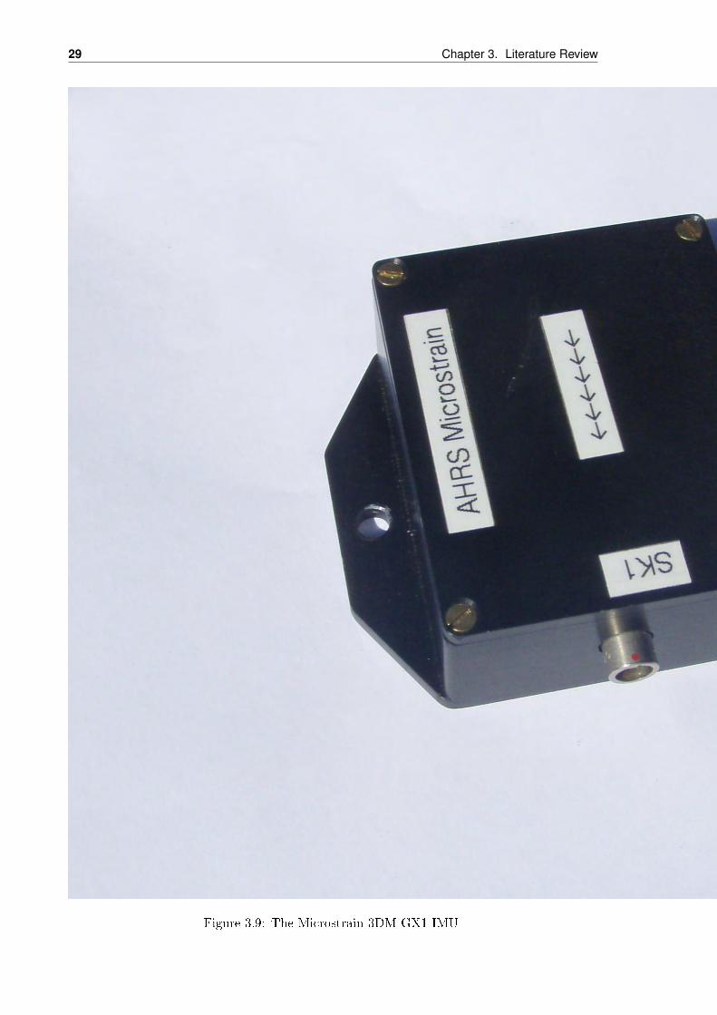
29 Chapter 3. Literature Review
Figure 3.9: The Microstrain 3DM-GX1 IMU

3.4. State Estimation and Measurement 30
Figure 3.10: The gyroscope assemblyVerplaetse (1996)
Accelerometer Errors The variation in temperature causes the properties of the polysili-
con springs in the accelerometers to change, thus introducing a bias. However, the 3DM-GX1
encorporates readings from an onboard thermometer which virtually eliminate these tempera-
ture eects MicroStrain (2006). Due to the natural resonances of the accelerometer structure,
the dynamic response of the accelerometers is poor. The 3DM-GX1 corrects for this (to a
limited extent) by passing the raw accelerometer data through a low-pass lter. Another er-
ror in the acceleration readings is due to non-orthogonality of the three accelerometers during
construction. The 3DM-GX1 quotes this bias at a maximum of 0.2% over a wide temperature
range, however no correction is provided for this error.
Gyroscope Errors The variation in temperature alters the stiness of the tines and dither
frame within the gyroscope (refer to Figure 3.10), thus introducing an error in the scale of
the angular rate reading. Again, the 3DM-GX1 encorporates readings from the onboard
thermometer to attempt to eliminate these temperature eects [3DM-GX1 2006]. In contrast
to the accelerometers, the gyroscopes provide accurate dynamic results, but an innacurate
static response. To improve the static response, the 3DM-GX1 fuses the gyroscope data with
the data from the magnetometers, which has a good static response. Non-orthogonality of
the three gyroscopes, caused during construction, is also an issue. The 3DM-GX1 quotes this
bias at a maximum of 0.2% over a wide temperature range, however no correction is provided
for this error. The nal error is due to saturation of the gyroscope angular rate reading. This
occures at 300 degress per second, however since it is impossible for a vehicle to rotate this

31 Chapter 3. Literature Review
Figure 3.11: The Honeywell GT1 Series 1GT101DC Solid State Hall-Eect Sensor(Honeywell)
quick, this facet is not seen as a problem.
Magnetometer Errors Temperature has no eect on Fluxgate magnetometers. Rather,
distortions on the local magnetic eld, such as those caused by rotating machinery and certain
stationary metals may cause any angle of magnetometer error bias. The 3DM-GX1 cannot
correct for these errors, therefore the inly solution is to ensure that the unit is kept away from
any such anomolies. Missalignment during conbstruction again accounts for an error of 0.4%
(MicroStrain, 2006).
The Hall-Effect Sensor
There are two broad categories of Hall-Eect sensors: those with magnetic pickups and those
with non-magnetic pickups. The Honeywell GT1 Series 1GT101DC Solid State Hall-Eect
Sensor, shown in Figure 3.11, uses non-magnetic pickups, therefore this design and any inher-
ent aws are discussed.
Non-magnetic pickup hall eect sensors create and monitor a magnetic eld. Any ferrrous
object in close proximity causes distortion of the eld and is therefore sensed. The Honeywell
GT1 Series 1GT101DC Solid State Hall-Eect Sensor uses this principal to trigger the rising

3.4. State Estimation and Measurement 32
Figure 3.12: The ETI Systems 10-Turn Wire-Wound 1 kΩ Rated Precision Potentiome-ter(Systems, 2006)
edge of the units output voltage. This sensor is installed facing the universal joint of the
tailshaft of the TARGET vehicle (discussed in greater detail in section [insert section]). The
sensor has a good low speed response and a bandwidth greater than 3600 RPM (Honeywell),
which corresponds to a much faster frequency than the tailshaft of the TARGET can spin at.
Therefore the sensor is predicted to be able to determine any speed that the hall eect sensor
outputs. It also bears mentioning that the pulse wave output from the sensor is converted to
an analogue voltage as this is the most convinient form to input to the TARGET computer.
A likely error, therefore, is analogue noise on the voltage signal due to sources such as the
vehicle distributor, starter motor and other power sources. This error may be modelled as
Gaussian noise with a zero-mean distribution.
The Potentiometer
The potentiometer is by far the simplest sensor required in the TARGET vehicle. The sensor
functions when a voltage is applied to the terminals. The output voltage from the sensor is
proportional to the angular position of the sensor. The sensor is an ETI Systems 10-Turn
Wire-Wound 1 kΩ Rated Precision Potentiometer, shown in Figure 3.12, and is mounted via
a belt connection to the steering column.
The potentiometer is capable of turning 10 times, which is envisaged to be sucient to sense
the TARGET steering column fully locked in both directions. Sensor fatigue is also not
envisaged to be an issue since the sensor has a 25000 cycle lifespan (Systems, 2006). However,
electrical noise on the analogue output voltage is likely to be the major source of error from the

33 Chapter 3. Literature Review
potentiometer, since the output cable runs through the TARGET vehicle cabin, near several
motors and the distributor. This error may be modelled as Gaussian noise with a zero-mean
distribution.
3.4.2 Kalman Filter Comparison
As has already been mentioned, the process of State Estimation and Measurement involves
improvement of sensor data in real-time, to produce a set of states which may be used to
perform automatic control. Based on the errors presented in Section 3.4.1 (in particular the
GPS dropout) the sensor data will require fusion if observability is to be maintained. Also
a form of ltering will be required, to remove the noise in virtually all of the signals. The
Kalman Filter, developed by Rudolph Kalman in 1960 Welch and Bishop (2001), acheives
all of these things. For these reasons vehicles which use the above sensor suite typically
employ Kalman Filters (Vest, 2005; Brogdon et al., 2005). Kalman Filters are essentially a
set of iterative equations which run in real-time and attempt to combine sensor data into an
optimal estimate of the vehicle states. Kalman lters come in many forms and these are listed
in table 3.1.
This table is used later for the purpose of selecting a Kalman Filter for implmentation in the
TARGET vehicle.
3.4.3 Earth Coordinate systems
The OEM4-G2 Global Poitioning System sensor avaliable to this project has the capacity to
output data in two coordinate systems, or datums: the Earth-Centered Earth-Fixed (ECEF)
datum and the Geodetic datum. If data, referenced to either of these datums, is required for
state updates by the Kalman Filter, then the datum of the data must rst be transformed to
the Tangent Plane datum. These three datums are now described.
The Earth Centered Earth Fixed (ECEF) Datum
The ECEF datum comprises three orthogonal axes whose origin is the Earth's center of
mass, as shown in Figure 3.13. The X-Axis passes through the intersection of the Greenwich
Meridian and the Equator, the Z-Axis is parallel to the rotational axis of the Earth and
passes through the North Pole, and the Y-Axis is dened such that the coordinate system is
right-handed. The locations at which the coordinate axes penetrate the surface of the Earth
remain constant for all orientations of the Earth, i.e. the coordinate axes turn as the Earth
turns Xu (2003).

3.4. State Estimation and Measurement 34
Table 3.1: Kalman Filter comparisonsKalman Filter Type Advantages Dissadvantages
Linear• Provides an optimalestimate of the states(minimising sensornoise) Kelly (1994a).
• Precalculation of ltermatrices reduces compu-tational burden Carlson(2004), Rezaei and R.(2003).
• Easily understood andimplemented
• Only applicale to sys-tems of purely linearrelationships Conner(2000), p31.
• Noise must be zero-mean, white andGaussian Rezaei andR. (2003), p2.
Extended
• Applicable to both linearand non-linear systemsConner (2000),p 32.
• Reletively easily under-stood and implemented
• Not a formally opti-mal solution Zhao et al.(2003).
• Only reliable for systemswhich are almost linearon the time scale of up-date intervals Julier andJK (1997).
• Noise errors accumulategradually over time Ma-tia et al. (2006).
Unscented
• Noise is not assumed tobe Gaussian Julier andJK (1997).
• Superior performance tothe Extended KalmanFilter Julier and JK(1997).
• The mean and covari-ance properties of thenoise are calculatedthrough the unscentedprocess and thereforeneed not be known inadvance
• Dicult to understandand implement
Fuzzy
• Noise is not assumed besymetrically distributedabout the mean Matiaet al. (2006).
• Noise errors may beforced not to accumu-late over timeMatia et al.(2006)
• The process is computa-tionally expensive

35 Chapter 3. Literature Review
Figure 3.13: The Earth-Centered Earth-Fixed Datum

3.4. State Estimation and Measurement 36
Figure 3.14: The Geodetic Datum
The Geodetic Datum
The Geodetic Coordinate System, shown in Figure 3.14, comprises three dimensions - Lati-
tude, φ, Longitude, λ, and Height, h. The denitions of these three Geodetic dimensions rely
on a construction line which passes through the point of interest at a normal to the surface
of the Earth. This line is hereby referred to as the Normal Line. Latitude is dened as the
angle between the plane of the Equator and the Normal Line and is positive for points which
lie above the Equator (i.e. the North Pole has a Latitude of 90o). Longitude is dened as the
angle between the projection of the Grenwich Meridian onto the plane of the Equator and the
projection of the Normal Line onto the plane of the Equator and spans −180o to 180o. TheGeodetic Height is dened as the distance from the surface of the earth (at mean sea level)
to the point of interest along the Normal Line Xu (2003).

37 Chapter 3. Literature Review
Figure 3.15: The Tangent Plane
The Tangent Plane
The Tangent Plane, shown in Figure 3.15, simply consists of a plane, tangential to the surface
of the Earth at the point of interest. Three axes dene the the Tangent Plane Datum, namely
the North axis, N , which points along the lines of constant latitude, the East axis, E, which
points along the lines of constant longitude and the Height, H, which is dened exactly
the same for the Tangent Plane Datum as for the Geodetic Datum Herrington (1995). The
Tangent Plane is useful since each of the axes are measured in meters, an SI unit which is
required for most calculations. If the Tangent Plane is continuously resolved for a moving
object then this coordinate frame simply maps the ellipsoid of the Earth to a plane.
3.5 Autonomous Guidance Control
The Autonomous Guidance Control section of the TARGET project encompasses the devel-
opment and systems-integration of an autonomous waypoint-based guidance controller for
the ground target vehicle. The following section presents the results and recommendations
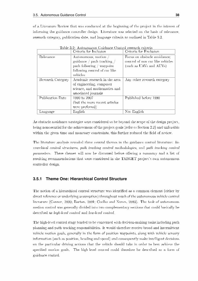
3.5. Autonomous Guidance Control 38
of a Literature Review that was conducted at the beginning of the project in the interest of
informing the guidance controller design. Literature was selected on the basis of relevance,
research category, publication date, and language criteria as outlined in Table 3.2.
Table 3.2: Autonomous Guidance Control research criteriaCriteria for Inclusion Criteria for Exclusion
Relevance Autonomous, motion /guidance / path tracking /path following / waypointfollowing control of car-likevehicles
Focus on obstacle avoidance;control of non-car-like vehicles(such as UAVs and AUVs)
Research Category Academic research in the areaof engineering, computerscience, and mathematics andassociated journals
Any other research category
Publication Date 1990 to 2007(but the more recent articleswere preferred)
Published before 1990
Language English Not English
As obstacle avoidance strategies were considered to be beyond the scope of the design project,
being nonessential for the achievement of the project goals (refer to Section 2.2) and unfeasible
within the given time and monetary constraints, this further reduced the eld of review.
The literature analysis revealed three central themes in the guidance control literature: hi-
erarchical control structures, path tracking control methodologies, and path tracking control
parameters. These themes will now be discussed before oering a summary and a list of
resulting recommendations that were considered in the TARGET project's own autonomous
controller design.
3.5.1 Theme One: Hierarchical Control Structure
The notion of a hierarchical control structure was identied as a common element (either by
direct reference or underlying assumption) throughout much of the autonomous vehicle control
literature (Conner, 2000; Barton, 2001; Coelho and Nunes, 2003). The task of autonomous
motion control was generally divided into two complementary sections that could basically be
described as high-level control and low-level control.
The high-level control stage tended to be concerned with decision-making tasks including path
planning and path tracking responsibilities. It would therefore receive broad and intermittent
vehicle motion goals, generally in the form of position waypoints, along with vehicle sensory
information (such as position, heading and speed) and consequently make intelligent decisions
on the particular driving actions that the vehicle should take in order to best achieve the
specied motion goals. The high-level control could therefore be described as a form of
guidance control.

39 Chapter 3. Literature Review
The low-level control stage, on the other hand, was generally responsible for implementing
the desired vehicle actions as determined by the high-level controller. Such action / motion
execution control would therefore regulate the control of the vehicle actuators (such as steering,
brake, and throttle motors) in order to safely, accurately and rapidly achieve the particular
vehicle motion setpoints provided by the high-level guidance controller (such as steering angle
and vehicle speed commands). Thus the high-level decision-based guidance control and the
low-level action-based motion execution control work together in series to provide a holistic
autonomous control of vehicle motion. Such hierarchical control architecture also clearly
reects a traditional conception of the general automatic control paradigm the perception
- decision - action philosophy (Fraichard, 2001). Thus for the purposes of the TARGET
vehicle project, the Autonomous Guidance Control section is concerned with the design of a
high-level decision-making guidance controller, whereas the lower-level action control is the
responsibility of the Motion Execution Control task (which is discussed in Sections 3.6 and
6.3).
3.5.2 Theme Two: Path Tracking Control Methodologies
Having identied the general architecture that underlies much of the autonomous vehicle
control literature, it is appropriate to enter into a discussion of the generic systems that have
been suggested and developed for such an application. Suárez et al. (2003) have loosely divided
path tracking control systems into two main categories which they refer to as temporal and
spatial. The temporal label has been used to designate autonomous motion control regimes
that are based on the direct application of standard control theory in which the goal is to
reach a specied location at a specied time. Spatial, on the other hand, refers to control
regimes which stem more from geometric relationships, in which the goal is to simply stay as
close as possible to a specied geometric path (Egerstedt et al., 2001). However, this is not
necessarily a strict separation as many strategies combine both spatial and temporal aspects
to varying degrees. In the proceeding discussion some of the common spatial and temporal
autonomous motion control regimes will be introduced.
3.5.2.1 Spatial Regimes
The spatial category incorporates a range of motion control strategies which are known broadly
as pursuit techniques. Many geometric pursuit techniques and variations have been developed
for path tracking control including (in increasing complexity):
• follow-the-carrot (Barton (2001); Golconda (2005)),
• pure pursuit (Kelly (1994a); Mörtberg (2006); Caravita et al. (2007); Barton (2001)),
• and vector pursuit (Wit et al. (2004); Mörtberg (2006); Barton (2001)).
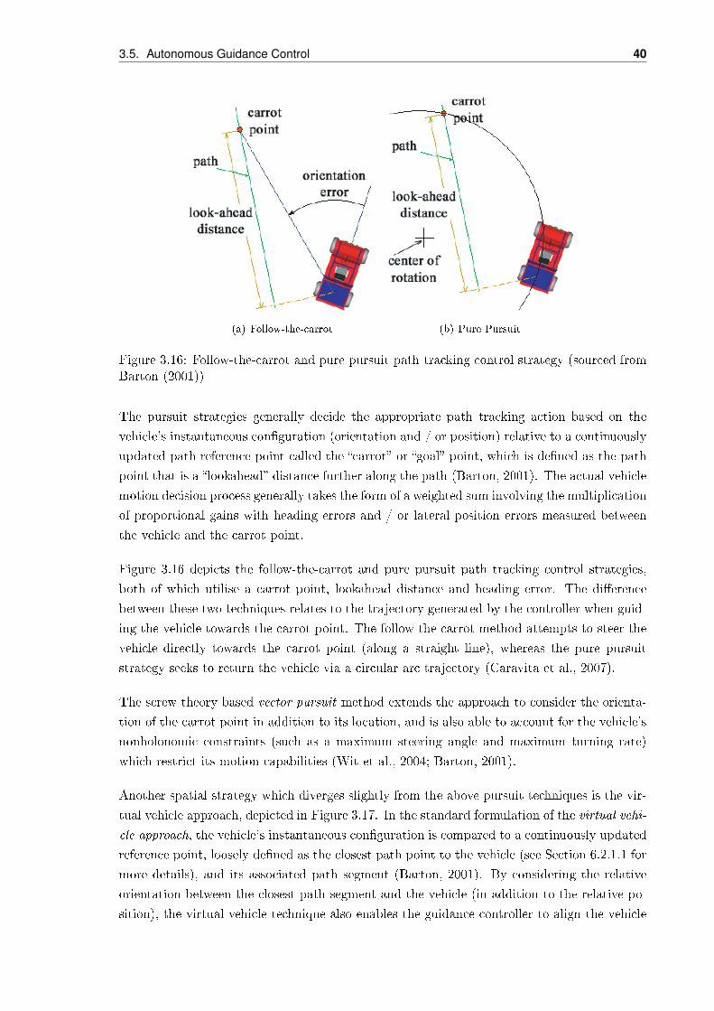
3.5. Autonomous Guidance Control 40
(a) Follow-the-carrot (b) Pure Pursuit
Figure 3.16: Follow-the-carrot and pure pursuit path tracking control strategy (sourced fromBarton (2001))
The pursuit strategies generally decide the appropriate path tracking action based on the
vehicle's instantaneous conguration (orientation and / or position) relative to a continuously
updated path reference point called the carrot or goal point, which is dened as the path
point that is a lookahead distance further along the path (Barton, 2001). The actual vehicle
motion decision process generally takes the form of a weighted sum involving the multiplication
of proportional gains with heading errors and / or lateral position errors measured between
the vehicle and the carrot point.
Figure 3.16 depicts the follow-the-carrot and pure pursuit path tracking control strategies,
both of which utilise a carrot point, lookahead distance and heading error. The dierence
between these two techniques relates to the trajectory generated by the controller when guid-
ing the vehicle towards the carrot point. The follow-the-carrot method attempts to steer the
vehicle directly towards the carrot point (along a straight line), whereas the pure pursuit
strategy seeks to return the vehicle via a circular arc trajectory (Caravita et al., 2007).
The screw theory based vector pursuit method extends the approach to consider the orienta-
tion of the carrot point in addition to its location, and is also able to account for the vehicle's
nonholonomic constraints (such as a maximum steering angle and maximum turning rate)
which restrict its motion capabilities (Wit et al., 2004; Barton, 2001).
Another spatial strategy which diverges slightly from the above pursuit techniques is the vir-
tual vehicle approach, depicted in Figure 3.17. In the standard formulation of the virtual vehi-
cle approach, the vehicle's instantaneous conguration is compared to a continuously updated
reference point, loosely dened as the closest path point to the vehicle (see Section 6.2.1.1 for
more details), and its associated path segment (Barton, 2001). By considering the relative
orientation between the closest path segment and the vehicle (in addition to the relative po-
sition), the virtual vehicle technique also enables the guidance controller to align the vehicle

41 Chapter 3. Literature Review
Figure 3.17: Virtual Vehicle spatial guidance control strategy
with the path orientation rather than simply guiding the vehicle directly towards a particular
position on the path (which inherently leads to overshoot problems). This essentially enables
much smoother and intuitive path following ability.
3.5.2.2 Temporal Regimes
The so-called temporal path tracking regimes can be loosely subdivided into control systems
that contain a kinematic or dynamic mathematical vehicle model and those which do not
(Castaño et al., 2004). Typically, temporal path tracking control systems, whether math-
ematical or non-mathematical, operate on errors between xed (waypoint-dened) vehicle
state commands and the actual measured states of the vehicle (such as position, heading,
and speed).
The mathematical category of temporal path tracking regimes describes a variety of state-
space techniques including the Linear Quadratic Regulator / LQR (Bevly et al. (2002); Naeem
et al. (2003)) and other linear (Coelho and Nunes, 2003) and non-linear (Switkes and Gerdes,
2005; Cordesses et al., 2000; Sharp et al., 2000) control laws. If provided with an accurate
mathematical vehicle model, such controllers are capable of very high precision path following
(Barton, 2001). However, building an accurate mathematical model of a non-linear, high
dimensional system can also be a dicult and labour-intensive task.
The other temporal category includes control systems based on the application of fuzzy logic
or neural networks, which do not require an explicit mathematical vehicle model and yet
are capable of providing control over highly non-linear processes including that of vehicle
guidance (Fraichard, 2001). Such systems tend to be based on rules formed from expert or
experiential knowledge of process behaviour, which in this case is vehicle driving behaviour.
These rule sets can become quite large for complex processes, and as a result the fuzzy control
styled approach can be relatively computationally expensive compared to some of the other
methods, though this varies depending on the choice of rule arbitration technique.

3.5. Autonomous Guidance Control 42
3.5.3 Theme Three: Path Tracking Control Parameters
While the literature's range of overarching path tracking control methodologies has been
reviewed, the discussion will now turn to the particular control parameters that have been
used within these strategies. It is worth rst noting that while high-level steering control has
been given extensive coverage throughout the autonomous motion control literature, high-
level speed guidance has received little attention. Rather, there seems to be a dominating
assumption that speed commands should simply be supplied along with position waypoints
(for example Holden (2004)). In some of the literature saturation / limiting has been described
as a means of ensuring that steering decisions are appropriate (and safe) given the vehicle's
speed (Kelly, 1994a; Sharp et al., 2000; Golconda, 2005). This is a gap in the current literature
that deserves to receive greater attention. Thus the control parameters presented in this
section are based on the steering component of autonomous guidance control alone, though
some may also prove to be useful for speed guidance.
In the case of typical temporal control strategies the control parameters tend to simply be
the errors between the desired and actual vehicle states (such as position, orientation, and
speed). The spatial control strategies, however, naturally extend the possibilities of parameter
selection beyond the pure vehicle states and have therefore been found to have a variety
of parameters represented within the autonomous motion control literature. A number of
common spatial control parameters include cross-track error, heading error, and various forms
of feedforward.
3.5.3.1 Cross-track Error
As identied in Figure 3.18, the cross-track error, d⊥, (with a number of synonyms including
lateral deviation) is a term for the perpendicular distance from the relevant path point or
segment to the origin of the vehicle coordinate frame (Holden, 2004; Elkaim et al., 2006).
It is therefore basically a measure of the position error between the vehicle and the path.
Consequently, a guidance controller equipped with a cross-track control parameter attempts
to minimise the cross-track error and thereby return the vehicle to the desired path.
Proportional control of the cross-track error was the most common (Holden, 2004; Sharp
et al., 2000), however PI (proportional plus integral) control was presented in Suárez et al.
(2003) and also Elkaim et al. (2006). The added integral control had the advantage (in typical
fashion) of alleviating any steady-state cross-track error which prevents the error from being
driven to zero even after the control signal has settled (Suárez et al., 2003).
3.5.3.2 Heading Error
Heading error (or orientation error '), θe, as indicated in Figure 3.18, was another control
parameter frequently incorporated into path tracking controller designs. The particular con-
struction of the heading error depended on the overarching control strategy. In all cases, the

43 Chapter 3. Literature Review
Figure 3.18: Spatial guidance control parameters of cross-track error, d⊥, and heading error,θe
rationale of heading control was to direct the vehicle to the desired path, but in some cases
(such as with the virtual vehicle approach and vector pursuit) the objective was extended
to also returning the vehicle with an orientation that matched that path that is, to ap-
proach the desired path asymptotically. Control of heading error tended to be implemented
as proportional control (Sharp et al., 2000; Elkaim et al., 2006). However, a PID controller
for producing steering direction setpoints based on heading error was described in Golconda
(2005).
3.5.3.3 Feedforward Terms
In a number of cases the guidance controllers in the literature incorporated a feedforward
component to their path tracking. In relation to path tracking, feedforward generally refers
to the variety of path preview strategies that can be used to provide anticipatory path follow-
ing motion commands. It can also be used to account for delays in the implementation of the
control signal (Mörtberg, 2006). Without a feedforward term, the autonomously controlled
vehicle will tend to lag behind the desired path (especially when cornering) as the control
system can only produce a control action once there is an error between the vehicle congura-
tion and the path point or path segment (Barton, 2001). Appropriate feedforward terms can
eliminate this lagging behaviour by ensuring that the appropriate corrective action is taken
before the vehicle actually deviates from the path.
A basic form of feedforward control is inherent in the pursuit techniques that were previ-
ously described (Section 3.5.2.1) since the control action is determined by reference to a path
point (carrot point) that is a lookahead path distance beyond the vehicle. However, more
complicated feedforward strategies were also present in the literature. Sharp et al. (2000);

3.5. Autonomous Guidance Control 44
Figure 3.19: Simulated path following using a feedback controller (sourced from Barton(2001))
Sharp and Valtetsiotis (2001); Castaño et al. (2004) and Switkes and Gerdes (2005) all utilise
a feedforward technique based on a projected cross-track error. Barton (2001), on the other
hand, oers a feedforward parameter which is an estimate of the average steering angle of an
upcoming number of path segments. Barton (2001) has recorded signicant improvements of
this feedforward approach over equivalent feedback systems, as can be seen from a comparison
of the simulated results depicted in Figure 3.19 and Figure 3.20.
3.5.4 Summary and Recommendations
The Autonomous Guidance Control Literature Review has identied and discussed three
main themes relating to the guidance control of a car-like vehicle. The rst was the use of
hierarchical control structures in which a high-level decision-making autonomous guidance
controller feeds vehicle motion setpoints into a lower-level motion execution controller which
in turn implements the motion setpoints by controlling the vehicle actuators. The second
theme was that of path tracking control methodologies which could be separated into spatial
(associated with geometry) and temporal (generated by standard control theory) strategies.
The nal theme introduced three commonly identied spatial path tracking control parameters
cross-track error, heading error, and various forms of feedforward.
In light of this review, the following recommendations were made for the TARGET project's
autonomous control task:
• The autonomous control be endowed with a hierarchical control structure in which a
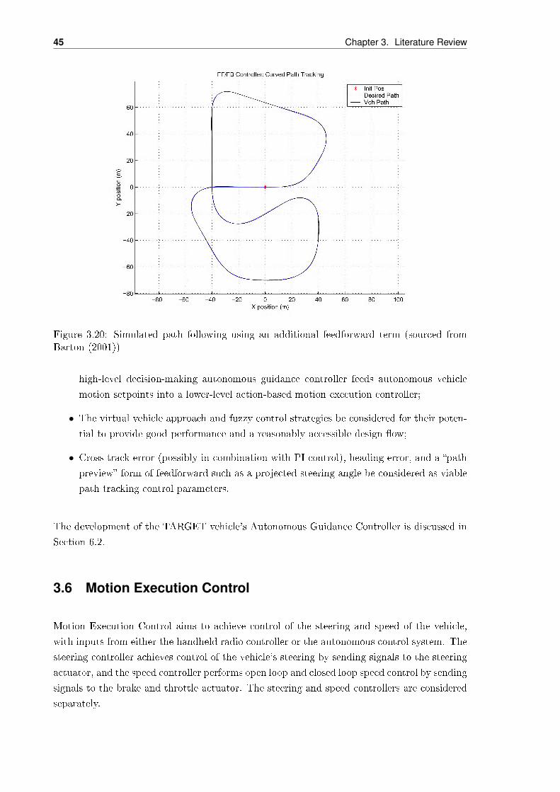
45 Chapter 3. Literature Review
Figure 3.20: Simulated path following using an additional feedforward term (sourced fromBarton (2001))
high-level decision-making autonomous guidance controller feeds autonomous vehicle
motion setpoints into a lower-level action-based motion execution controller;
• The virtual vehicle approach and fuzzy control strategies be considered for their poten-
tial to provide good performance and a reasonably accessible design ow;
• Cross-track error (possibly in combination with PI control), heading error, and a path
preview form of feedforward such as a projected steering angle be considered as viable
path tracking control parameters.
The development of the TARGET vehicle's Autonomous Guidance Controller is discussed in
Section 6.2.
3.6 Motion Execution Control
Motion Execution Control aims to achieve control of the steering and speed of the vehicle,
with inputs from either the handheld radio controller or the autonomous control system. The
steering controller achieves control of the vehicle's steering by sending signals to the steering
actuator, and the speed controller performs open loop and closed loop speed control by sending
signals to the brake and throttle actuator. The steering and speed controllers are considered
separately.
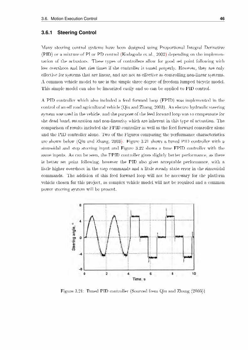
3.6. Motion Execution Control 46
3.6.1 Steering Control
Many steering control systems have been designed using Proportional Integral Derivative
(PID) or a mixture of PI or PD control (Kodagoda et al., 2002) depending on the implemen-
tation of the actuators. These types of controllers allow for good set point following with
low overshoot and fast rise times if the controller is tuned properly. However, they are only
eective for systems that are linear, and are not as eective at controlling non-linear systems.
A common vehicle model to use is the simple three degree of freedom lumped bicycle model.
This simple model can also be linearized easily and so can be applied to PID control.
A PID controller which also included a feed forward loop (FPID) was implemented in the
control of an o road agricultural vehicle (Qiu and Zhang, 2003). An electro-hydraulic steering
system was used in the vehicle, and the purpose of the feed forward loop was to compensate for
the dead band, saturation and non-linearity which are inherent in this type of actuation. The
comparison of results included the FPID controller as well as the feed forward controller alone
and the PID controller alone. Two of the Figures comparing the performance characteristics
are shown below (Qiu and Zhang, 2003). Figure 3.21 shows a tuned PID controller with a
sinusoidal and step steering input and Figure 3.22 shows a tune FPID controller with the
same inputs. As can be seen, the FPID controller gives slightly better performance, as there
is better set point following, however the PID also gives acceptable performance, with a
little higher overshoot in the step commands and a little steady state error in the sinusoidal
commands. The addition of this feed forward loop will not be necessary for the platform
vehicle chosen for this project, as complex vehicle model will not be required and a common
power steering system will be present.
Figure 3.21: Tuned PID controller (Sourced from Qiu and Zhang (2003))

47 Chapter 3. Literature Review
Figure 3.22: Tuned FPID controller (Sourced from Qiu and Zhang (2003))
3.6.2 Throttle / Brake Switching Logic
The speed controller will control the speed of the vehicle by actuating both the throttle and
brake pedal. The speed controller design requires that the throttle and brake are not actuated
simultaneously. This is to ensure that speed control is smooth, and extra wear and tear on
the braking system is avoided. So switching logic must be incorporated in the system. Speed
controller designs in literature have implemented switching logic by applying a boundary layer
to a switching line (Kwon et al., 2001). The switching line indicates the acceleration of the
vehicle when both actuators are in their minimum position, for any speed. Throttle control
is used when the desired acceleration is above the switching line, and brake control is used
when the desired acceleration is below. Switching between controllers only occurs when the
desired acceleration is not within the boundary layer. The boundary layer is a small area on
either side of the switching line. Controller switching does not occur while in the boundary
layer to prevent frequent switching between throttle and brake control. Figure 3.23 illustrates
the controller switching logic, with the switching line (line of minimum acceleration) and
boundary layer.
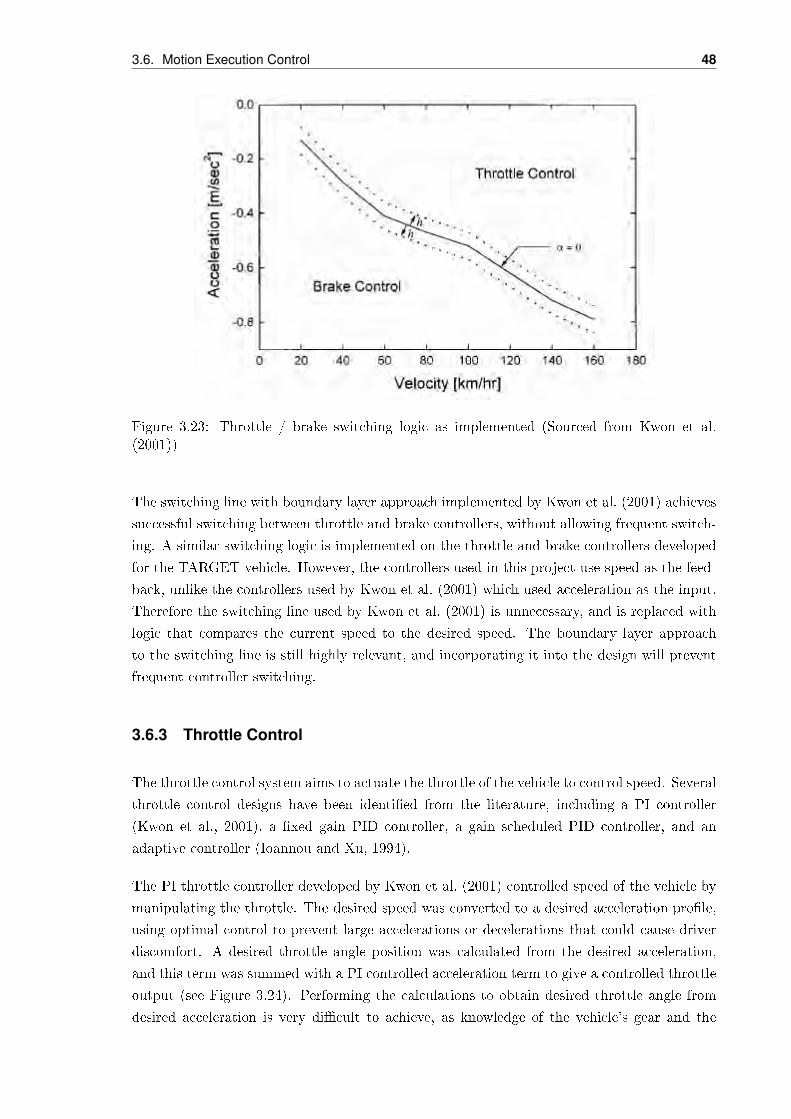
3.6. Motion Execution Control 48
Figure 3.23: Throttle / brake switching logic as implemented (Sourced from Kwon et al.(2001))
The switching line with boundary layer approach implemented by Kwon et al. (2001) achieves
successful switching between throttle and brake controllers, without allowing frequent switch-
ing. A similar switching logic is implemented on the throttle and brake controllers developed
for the TARGET vehicle. However, the controllers used in this project use speed as the feed-
back, unlike the controllers used by Kwon et al. (2001) which used acceleration as the input.
Therefore the switching line used by Kwon et al. (2001) is unnecessary, and is replaced with
logic that compares the current speed to the desired speed. The boundary layer approach
to the switching line is still highly relevant, and incorporating it into the design will prevent
frequent controller switching.
3.6.3 Throttle Control
The throttle control system aims to actuate the throttle of the vehicle to control speed. Several
throttle control designs have been identied from the literature, including a PI controller
(Kwon et al., 2001), a xed gain PID controller, a gain scheduled PID controller, and an
adaptive controller (Ioannou and Xu, 1994).
The PI throttle controller developed by Kwon et al. (2001) controlled speed of the vehicle by
manipulating the throttle. The desired speed was converted to a desired acceleration prole,
using optimal control to prevent large accelerations or decelerations that could cause driver
discomfort. A desired throttle angle position was calculated from the desired acceleration,
and this term was summed with a PI controlled acceleration term to give a controlled throttle
output (see Figure 3.24). Performing the calculations to obtain desired throttle angle from
desired acceleration is very dicult to achieve, as knowledge of the vehicle's gear and the

49 Chapter 3. Literature Review
engine map is required. The PI throttle controller achieved satisfactory control of vehicle
acceleration. Test results for step inputs to the controller are shown in Figure 3.25. Note that
the slow rise times of the vehicle's speed are desirable in this case to avoid driver discomfort.
Figure 3.24: PI throttle controller block diagram (Sourced from Kwon et al. (2001))
Figure 3.25: PI throttle controller test results (Sourced from Kwon et al. (2001))
The xed gain and gain scheduled PID controllers developed by Ioannou and Xu (1994) used
a slightly dierent approach to the PI throttle controller. The xed gain PID controller
simply introduced a derivative error term. The gain scheduled PID controller improved on
the performance of the xed gain controller by scheduling the gain for dierent operating
points. The method of gain scheduling was used to provide tuned gains for various operating
points, to overcome the problem of non-linearity. Test results for the two controllers found
in the literature show similar responses, and were considered satisfactory in both cases. The
xed gain controller was found to be slightly inferior to the gain scheduled controller, due to
oscillations in acceleration and driver discomfort at low speeds.
The adaptive controller developed by Ioannou and Xu (1994) was designed to provide a speed
controller that was self-adapting to the system parameters. The controller structure was too
complicated to be considered for use in the project. Test results for the controller showed a
response superior to the xed gain and gain scheduled PID controllers.
Four controller structures for the throttle were identied; a PI controller, a xed gain PID
controller, a gain scheduled PID controller, and an adaptive controller. As all controllers
achieved satisfactory control of the vehicle's speed, a classical control structure is clearly
adequate for the application.

3.7. Path Generation 50
3.6.4 Braking Controller
An intelligent cruise control (ICC) system was developed as a joint eort between Hanyang
University in South Korea and the Hyundai motor company using a feed forward plus PID
control for the braking system (Kwon et al., 2001). The aim of the system was to provide
for cruise control with sensors to measure the distance to the next vehicle in front of the
development vehicle. If the gap between the two vehicles grew too small, the ICC would act to
increase this gap to a safe distance. Hence, this provides an ICC system which maintains a safe
distance between the development vehicle and the next vehicle ahead. The PID controller is
used to provide good set point following and to allow for fast response and settling times. PID
control usually gives very good performance in linear systems, but do not work very eectively
in non-linear systems. The feed forward loop is used to overcome the non-linear nature of this
system. This type of controller is fairly easy to implement and has a good response, however
the system's dynamic response must be known accurately to create a nonlinear system model.
The performance characteristics of this controller are shown below in Figure 3.26. In this
situation, a vehicle traveling at 90 km/h is used to cut in front of the ICC vehicle traveling at
110 km/h at a distance of approximately 40 m. As can be seen, the braking controller works
to maintain the distance at 40 m. The performance of the controller is acceptable, with fast
set point tracking as seen in Figure 3.26 (c) and (e). The settling times are also fast, and
there is minimal overshoot.
Figure 3.26: PID plus feed forward performance characteristics (Sourced from Yi, et al. 2005)
3.7 Path Generation
Path generation for the vehicle is essential in maintaining good levels of control. The path
must be generated from a list of user specied waypoints. These calculations were originally

51 Chapter 3. Literature Review
Figure 3.27: Linear splines between waypoints (Lu, 2007)
to be carried out by the onboard target computer. However, path generation for the vehicle
was shifted into the base station computer for two reasons. The vehicle's onboard processor
will already be processing large amounts of data by running a Simulink model. Also, by
computing the path at the base station the path can be displayed to the user.
The method used must satisfy two conditions to be suitable for generating a path. Firstly,
the generated path should pass through every waypoint selected by the user. Some numerical
methods generate a function that does not directly pass through the specied points (Spath,
1974). Secondly, the path must be relatively smooth as the car cannot make instantaneous
turns. Any sharp points in the path will be dicult for the vehicle to navigate.
To create a path for the vehicle, splines must be dened between each point. There are
several dierent methods for dening splines and each method will produce a dierent result.
The simplest method is linear splines. Linear splines are simply straight lines drawn between
each point (see Figure 3.27). This method generates a path through every point, but is not
suitable in almost every other characteristic as the path is not dierentially continuous at
each waypoint. The generated path contains sharp deviations and would be dicult for the
vehicle to navigate.
An extension of this method is one which denes a set of linear splines, but then applies
curves between them. This method still generates a simple path but is getting closer to the
path shape required for the vehicle. This path however does not pass through the dened
waypoints. Another method xes this problem by applying pseudo points around the dened
waypoints (see Figure 3.28) before applying the curves. However, for this method to provide
a good path the pseudo points must be strategically placed to prevent a large overshoot. The
resulting path could be generated to give multiple solutions that are feasible but may not be
appropriate.
Two other methods investigated are more complicated requiring many iterations to nd a
solution. B Splines is one such method which uses successive cubic curves to generate a
smooth path. The resulting path is very smooth and continuous, but does not pass directly
through every waypoint dened by the user.

3.7. Path Generation 52
Figure 3.28: Inserting pseudo points to generate a path (Lu, 2007)
Figure 3.29: Natural cubic splines, identied as a suitable method of path generation
The nal method investigated is called Natural cubic splines. The path it generates is smooth,
continuous and passes through each of the dened waypoints. An example, with 12 waypoints
is shown below in Figure 3.29.
3.7.1 Open Path
To calculate natural cubic splines, each of the coordinates (longitude and latitude) must be
considered separately and a cubic polynomial is tted between each point. Each Yi (u) denesa cubic polynomial between waypoint coordinates yi and yi+1. This method is outlined in
Bartels et al. (1987), the solution for the coordinates can be found using Equation (3.1).

53 Chapter 3. Literature Review
Yi (u) = ai + biu+ ciu2 + diu
3
where
ai = yi
bi = Di
ci = 3 (yi+1 − yi)− 2Di −Di+1
di = 2 (yi − yi+1) +Di +Di+1
(3.1)
The values of Di are found by solving the system of Equations (3.2). The computational
technique for solving this system is also outlined in Bartels et al. (1987).
2 11 4 1
1 4 11 4 1
.... . .
. . .. . .
. . .. . .
. . .
1 4 11 2
D0
D1
D2
D3
...
Dn−1
Dn
=
3 (y1 − y0)3 (y2 − y0)3 (y3 − y1)
...
3 (yn−1 − yn−3)3 (yn − yn−2)3 (yn − yn−1)
(3.2)
The system must be solved twice to obtain a longitude and a latitude path approximation
between the given waypoints. The method produces n − 1 polynomials from n waypoints.
By repeating this process over the entire range of waypoints an array of cubic polynomials
can be obtained. When combined together these polynomials form the smooth path required.
Four boundary conditions must be satised to ensure each polynomial connects smoothly with
the next. These four boundary conditions are dened in Bartels et al. (1987) and shown in
Equations (3.3) to (3.6).
Yi (0) = yi (3.3)
Yi−1 (1) = yi (3.4)
Y′i−1 (1) = Y
′i (0) (3.5)
Y′′i−1 (1) = Y
′′i (0) (3.6)
3.7.2 Closed Path
One advantageous feature of the natural cubic splines is its ability to generate a closed path.
The majority of the automated driving competed by the vehicle will be done with a closed

3.8. Background Imagery 54
path.
A method outlined in Bartels et al. (1987) also allows a closed loop path for natural cubic
splines to be calculated. Computational techniques can be adapted from Spath (1974) and
are similar to the open path method (see Equation (3.2)). Instead the values of Di are found
by solving Equation (3.7).
4 1 11 4 1
1 4 11 4 1
.... . .
. . .. . .
. . .. . .
. . .
1 4 11 1 4
D0
D1
D2
D3
...
Dn−1
Dn
=
3 (y1 − yn)3 (y2 − y0)3 (y3 − y1)
...
3 (yn−1 − yn−3)3 (yn − yn−2)3 (y0 − yn−1)
(3.7)
Several factors can aect the overall path generated using the natural cubic splines. If long
distances are left between waypoints then a large overshoot can occur. Due to the methods
used in Equations (3.2) and (3.7) placing waypoints too close together will also produce a
path that is impossible for the vehicle to follow. By introducing extra, strategically placed,
waypoints into the system these problems can be overcome (illustrated in Figure (3.30)).
For the purposes of this application it is assumed the user can review the suitability of the
automatically generated path. If a path is not suitable, the user can redene waypoints until
a suitable path is generated.
3.8 Background Imagery
The background map is a critical part of the GUI. Without it the user would nd it very
dicult to input waypoints correctly and accurately. In order for a picture to appear cor-
rectly in the background the user must rst prepare the image, or at least know some crucial
information about the area in the picture.Several dierent processes can be used in order for
the base station to correctly display an image in the background.
Initially, only two dierent methods were identied for dening a background image. These
three methods are illustrated in Figures 3.31 and 3.32. The rst approach (see Figure 3.31)
requires the denition of just one point and two dimensions, two assumptions are also made.
The rst assumption is the position of the given point. It is assumed to be in the upper left
hand corner of the image. The second assumption is that north is at the top of the image.

55 Chapter 3. Literature Review
(a) The path is impossible for the vehicle to follow around waypoint number three and has a large overshootbetween waypoints 4 and 5 caused by the large distance between wayponts 5 and 1
(b) Introducing extra, strategically placed, waypoints improves the path prole. Waypoints 2, 4 and 8have been added.
Figure 3.30: The advantage of adding extra waypoints to construct a smooth and achieveablepath
Figure 3.31: The rst, and easiest, method for dening a background image. Dene a referencepoint and specify the height and width of the image. The top of the image is assumed to benorth.
The second approach (see Figure 3.32) requires the denition of three points and no requires
assumptions. The three points will be sucient to completely dene the location, orientation
and skew of the image on the screen.

3.9. RF Communications 56
Figure 3.32: The second, and more complicated method for dening a background image.Place three points on the image. The location, orientation and skew can all be dened bythese points.
Once the user has dened each background image and the conguration le has been gener-
ated, the images must be displayed onto the screen.
3.9 RF Communications
Wireless communications between the operator and the vehicle are by means of radio fre-
quencies. Short range RF communication is achieved by the use of handheld remote-controls
(handheld radio transmitters) operating at low frequencies while long range communications
require the use of RF modems operating at high frequencies. Details of both methods are
investigated to determine suitable devices that allow manual and autonomous operation of
the vehicle in short range and in long range respectively.
3.9.1 Handheld Remote-Control
The remote manual control operation of the vehicle can be compared to the way hobby aircraft
are controlled. The device for such control is the handheld remote-control (Figure 3.33) that
transmits data by emitting radio waves at low frequencies, typically in the range of 30 MHz
to 40 MHz. Further to the operation of the handheld remote-control is the transmission
of multiple sub-frequencies, also known as radio channels, where each channel is capable of
manipulating the dierent control surfaces of the hobby aircraft such as its ailerons, rudders
and elevators. The concept of controlling a number of control surfaces per radio channel may
be feasible in the project to manipulate the control aspects of the TARGET vehicle such
as speed, steering, transmission and possibly more, and hence achieving the goal of remote
manual control operations.

57 Chapter 3. Literature Review
Figure 3.33: A typical handheld remote-control (RF Innovations Ltd Pty, 2007)
3.9.1.1 AM vs FM
RC systems send data signals using either frequency modulation (FM) or amplitude modula-
tion (AM). FM systems encode a signal by varying the frequency of the carrier wave causing
compressions and rarefactions. The receiving end will decode the modulated frequency to
obtain the original signal. AM systems operate using a similar concept with the exception of
varying the amplitude instead of the frequency. Both FM and AM systems are susceptible
to interference that cause changes in amplitude; however the AM signals are further aected
as it relies on correct amplitude readings. However, since FM signals are independent of
amplitude variations, interference levels are minimal for FM signals. For this reason, modern
RC transmitters employ the FM system as it better rejects interference than AM systems.
Therefore it is recommended to select a frequency modulated hand held remote-control.
3.9.1.2 PPM vs PCM
Further to the frequency modulation system there are two ways of transmitting data signals.
These are Pulse Position Modulation (PPM) and Pulse Code Modulation (PCM). Although
PPM uses older technology than PCM, both are still readily used in today's market. The
dierences, advantages and disadvantages between PPM and PCM are summarised in Table
3.3. Despite signicant dierences between PPM and PCM, it is a matter of personal pref-
erence when deciding which system to operate; which is better determined with experience.
Some handheld remote-controls give options of both of the FM protocols (PPM and PCM)
and is recommended for the project.
3.9.1.3 Frequency Channels
A handheld remote-control has a number of radio channels that are used to send dierent
signals to its receiver. Instead of using these signals to control a model aircraft, the signals
can be manipulated to enable full access to the vehicle controls such as steering, speed, and

3.9. RF Communications 58
Table 3.3: Comparison of PPM and PCM Systems for handheld remote-controls (Rother,2007)
PPM PCM
inherently compact, simplecircuitry
Advantage: inexpensive
Can be small, complexcircuitry
Disadvantage: expensive
Analog technologyAdvantage: inexpensive andreceivers may be compatible
with dierent brandedtransmitters
Digital Technology(microprocessors)
Advantage: SophisticatedDisadvantage: must usereceiver of the same brandtype as its transmitter
Representation of signals arenot altered
Advantage: Servo motorswill move erratically at end oftransmission range, giving
early warning tot he operator.
Extremely accurate datasignals
Advantage: undisturbedservo movement
Disadvantage: lack of earlywarning signs can lead to
increased dilemmas
Momentary signal losses are'ironed out' due to inertia of
the physical system.Disadvantage: cannot
detect error hence false datais present
Has error checking(checksum) and fail safe
proceduresAdvantage: prevents falsedata signals and will stop too
short/long pulses fromdamaging servos as PPM
would
ignition. Each of these control aspects require a separate channel in order for it to operate
independently. After some experimentation in the laboratory, it was concluded that handheld
remote-controls transmit frequency channels of two dierent types: proportional and switch.
Proportional channels are represented by movable control sticks that are on the transmitter
where the frequencies are modulated continuously and in proportion to the positions of the
control sticks. The switch channel is represented by mechanical switches which manipulate
discrete data values. Today's market manufactures a multitude of handheld remote-controls
that typically has four proportional channels where any additional channels would be switch
channels.
3.9.2 RF Modems
Research shows that industrial applications which require long ranged wireless communica-
tions between their vehicles and base stations, nd their solution with RF modems. RF
modems are transceiver devices that modulate an analogue carrier signal to encode digital
information, and also demodulate such a carrier signal to decode the transmitted information
Nagrath (2007). RF modems are readily available on the market and are already being used to

59 Chapter 3. Literature Review
provide wireless communication solutions to such industries as mining and agriculture. A se-
lection of a suitable RF modem for the project requires sucient data transfer rate, reliability
and long range.
Figure 3.34: Caterpillar(TM) Trucks in open-pit mines (RF Innovations Ltd Pty, 2007)
The common requirement between the project and industrial applications is the need of wire-
less communications from a control base station to a mobile platform. Caterpillar(TM)trucks
(Figure 3.34), employed by mining companies, use RF modems to establish an eective com-
munication link from the mining area to the control station for critical vehicle status and
diagnostics. This establishes remote-control over dangerous mining operations in hostile en-
vironments.
Another use for RF modems is for autonomous control in automated processing industries, for
example, Patrick Corporation who implements an automated straddle carrier (Figure 3.35)
using RF modems. In this application RF modems provide a reliable wireless communication
link which was critical to moving cranes eectively and autonomously when required.
Figure 3.35: An Automated Straddle control system by the Patrick Corporation (RF Innova-tions Ltd Pty, 2007)
The two examples given here form the basis of the use of RF modems of similar features of the

3.9. RF Communications 60
project. Mining companies use RF modems to constantly monitor mining vehicles' statistics
and perform diagnostics which is very useful when implementing the TARGET vehicle. Since
the project also requires autonomous control of the TARGET vehicle, successful applications
such as the automated straddle control system gives condence that RF modems are most
suitable and reliable for the wireless communications in this project.
3.9.2.1 Modem Features
Most RF modems essentially have the same features that provide eective wireless communi-
cations. These include use of a spreading code, error checking, network protocols, data rates
and more. The more costly modems provide better quality in these features however there
are other dierences in RF modems that can be considered when selecting the most suitable
modem for the application. For example, the frequency range at which the modem operates
in.
The spreading code of RF modems refers to the way data signals are transmitted. RF modems
dier from the ordinary radio transmitting device by using modern technology known as the
Frequency Hopping Spread Spectrum (FHSS). Unlike ordinary radio transmitters, the FHSS
signal does not stay on one frequency but 'hops' between frequencies that only the dedicated
receiver can recognise and sync with the signals hopping pattern. The FHSS signals are then
resistant to interference and can prevent monitoring or jamming by third parties. Therefore
FHSS modems oer secure and robust communication links.
Error checking is another import feature of the RF modem. It contributes to the reliability
of the communication link because it attempts to prevent data packets from being lost or
corrupted. Due to the nature of radio communications, it is inevitable that some data can
be lost or corrupted, especially in hostile environments where other radio equipment is in
close proximity. Error checking procedures include Cyclic Redundancy Checking (CRC) that
constantly monitor the data trac for any abnormalities, and packet retransmissions for any
lost or corrupted data bits.
RF modems support a range of network protocols that allow exibility in its use in many
applications. Common protocols include point-to-point, point-to-multipoint, Hayes dial-up
and repeater. The point-to-point protocol only allows communications between two modems
(master and slave) whereas the point-to-multipoint protocol, also known as broadcasting,
allows communication from one master (the synchroniser) modem to multiple slave modems.
Hayes dial-up protocol oers a more powerful method of operation than the previous two
protocols as it allows dedicated communication between a master and one of many slaves.
RF modems mainly operate in the Industrial Scientic and Medical (ISM) band which includes
the typical 900 MHz and 2.4 GHz range. Operating at 900 MHz yields signicantly longer
range (approximately two times) than that is possible at 2.4 GHz (Maxstream Inc, 2007). In
comparison with the 900 MHz system, the 2.4 GHz system tends to readily malfunction in the

61 Chapter 3. Literature Review
vicinity of other 2.4 GHz devices and particularly in rainy conditions. It has some advantages
over the 900 MHz band as it only requires small antennas, making the system compact. Also,
the 2.4 GHz system is globally license-free whereas the 900 MHz systems are only permissible
in fewer countries. The 900 MHz band are utilised by radio modems in Supervisory Control
And Data Acquisition (SCADA) applications which provide high reliability, interference re-
jection and the longest range in hostile, industrial environments. Fortunately, Australia is
one of the few countries that provide license-free operations of 900 MHz systems hence this
is a viable option for the project.

3.9. RF Communications 62

Chapter 4
Hardware Design
4.1 The Van
Before work could begin on design and purchasing of any actuators a suitable vehicle plat-
form must be selected. The selection criteria was split into two sections. The rst detailed
requirements and the other detailed desired features. Each criteria was given a weighting
where required features were weighted most heavily with 10. The following weightings were
determined:
• Power steering (10) - Power steering was a denite requirement for the vehicle. It
allowed smaller actuators that would consume less power and be much cheaper than
larger actuators.
• Automatic gear shift (10) - The automatic gear shifter was also a denite requirement
as it would greatly reduce the complexity of gear shifting actuators.
• Correct price (10) - The allocated budget for the vehicle was $5000 so no vehicles beyond
this range should have been investigated.
• Adequate interior space for hardware (10) - To t the hardware (which is mainly stored
on the computer rack) adequate space is required. Vehicles with insucient space were
not investigated.
• Adequate exterior area (10) - To allow targeting of the vehicle by a UAV, an exterior area
of approximately nine square meters was required. Vehicles with inadequate exterior
area were not investigated.
• Good suspension (9) - Good suspension should ensure that the onboard hardware is not
damaged while driving on any rough roads the vehicle may encounter.
63
4.1. The Van 64
• Tight steering (8) - Tight steering will ensure the vehicle can be controlled as desired and
maintain its commanded course. However, as the absolute position of the vehicle can
be sensed, corrections for loose steering can be made, so this criterion was not critical,
hence the score of eight.
• Cargo barrier (8) - The cargo barrier will ensure that the equipment in the rear of the
vehicle will not harm the occupants of the cabin in a crash. If the vehicle did not already
come with a cargo barrier, then one could be purchased separately at signicant cost,
so a weighting of eight was appropriate.
• Low mileage (5) - Low mileage was desirable since a vehicle which has not traveled far
will be less likely to break down. However, breakdowns are quite unlikely based on this
criterion alone, so a weighting of ve was given.
• Good tires (8) - Good tires will ensure that the vehicle has a good grip on the road and
therefore can be controlled as commanded. However if the vehicle does not already have
good tires these can be purchased at signicant cost, therefore a weighting of eight was
given.
• No rust (9) - Rust, particularly on the mechanical components, causes weakening which
leads to breakages, thereby compromising the functionality of the vehicle. As it was
crucial for the success of the project that the vehicle runs, nine was allocated.
• Low electrical noise (4) - Low electrical noise will ensure that the electrical signals pass-
ing between hardware are not distorted. However if the vehicle does produce electrical
noise, particularly from the distributor, this could be compensated for by electrical
shielding of wires and components. Since electrical isolation will be implemented re-
gardless of the vehicle (i.e. the vehicle noise should incur no extra cost), this criterion
is weighted at four.
• Air conditioning (8) - Air conditioning should ensure that the control hardware remains
at a good temperature. This is quite important in rural Australia where high tempera-
tures are common.
• No logo decals (5) - The project does not wish to advertise by using the vehicle, so no
decal were permitted. However, decals could always be removed, after which repainting
is generally required, therefore a score of ve is allocated for the extra cost and eort
required.
• Valid registration (4) - To be driven on roads the vehicle must be registered. If the
vehicle did not come with registration, it must be purchased at a small cost. Therefore
a weighting of four was given.
While searching for a suitable vehicle these criteria were taken into consideration. After many
weeks of searching the range of possible vehicles identied was very small. Many vehicles
did not match one of the required (weighted 10) categories, with price being a major hurdle.

65 Chapter 4. Hardware Design
However, one vehicle was found that satised all of the required categories and was determined
to be suitable for the TARGET project's needs.
The identied vehicle was a Mitsubishi Express van. It had power steering, an automatic
transmission, adequate interior space and exterior area, no logo decals and air conditioning.
Several modications had made on the van for it to be fully functional. Figure 4.1 shows the
TARGET vehicle after these modications were made. The modications included:
• a service to remedy some minor smoke issues
• the installation of a cargo barrier
• the addition of the project and university insignia
Figure 4.1: The TARGET vehicle after being purchased and minor modications made
Once the vehicle was purchased the design, construction and installation of actuator could
begin.
4.2 TARGET Computer
The onboard computer is required to perform all of the computation required for control of
the van. A computer system compatible with MathWorks xPC Target was assembled to allow
the development of the program using this software package. The system includes four data
acquisition cards, a desktop computer, and other hardware.

4.2. TARGET Computer 66
4.2.1 xPC Target
MathWorks xPC Target is a rapid prototyping and hardware in the loop simulation environ-
ment. It enables Simulink models to be created on a host computer, and run in real time
on a target computer (the vehicle's onboard computer) with real input and output signals.
The xPC real time kernel handles the real time execution of the program, and is capable of
running the onboard computer program discussed in Section 6.1 at 50Hz. xPC Target has
been used in this project to enable the rapid development of all control systems for the vehicle
without requiring any programming in a low level language. The use of xPC Target imposes
several restrictions on the computer system hardware. The most signicant restriction is that
all data acquisition cards must be chosen from a relatively small list of supported devices.
To enable the deployment of the program on the vehicle's onboard computer, the xPC Target
Embedded Option was purchased. This is an extension to the xPC Target software, which
enables programs to be deployed as a stand-alone system. The stand-alone program created
with the embedded option boots from DOS, and runs without requiring a link to the host
computer.
4.2.2 Computer Hardware
The computer hardware consists of the computer itself and four peripheral I/O devices.
4.2.2.1 Computer
The onboard computer is a Pentium 4 desktop PC provided by Thales Australia. The com-
puter has a 2.8GHz Pentium 4 processor, and provides I/O expandability with ve PCI slots.
MathWorks xPC Target supports several form factors of computer hardware, including PCI,
compactPCI, and PC104. A PCI form factor has been used in this project predominantly
because a PCI computer was provided in-kind, but the form factor is also the fastest available
solution, and is supported with the cheapest and largest range of peripheral devices. A disad-
vantage of using a desktop PC is that it is not a particularly rugged platform. This has been
overcome by mounting the computer onboard the vehicle with foam for vibration damping.
4.2.2.2 Peripheral I/O devices
To meet the I/O requirements of the system, four peripheral I/O devices were purchased.
The I/O requirements comprises thirty nine signals - seven analogue inputs and one analogue
output, ve PWM inputs, twenty one lines of digital I/O, and four ports of RS232 serial
communications. A detailed list of the I/O signals is shown in Table 6.2. The four devices
purchased to meet these requirements are an analogue I/O card, a counter card, a digital I/O
card, and a RS232 serial communications card. The devices were chosen such that there is
room to interface more of each type of signal if the need arises.
67 Chapter 4. Hardware Design
• Analogue I/O card - PCI-6040E
A National Instruments PCI-6040E was chosen to fulll the analogue input and output re-
quirements of the system. This card has sixteen analogue inputs, two analogue outputs, two
counters, and eight lines of digital I/O. The PCI-6040E was chosen as it was the lowest cost
card that could provide an 8kHz analogue output for sound generation (see Section 6.1.6),
and could provide decoding for at least one PWM signal.
• Counter card - PCI-6601
A National Instruments PCI-6601 was chosen to provide decoding for four of the ve PWM
inputs to the computer. It has four counters with 32 bit resolution, each of which can decode
a single PWM. The PCI-6601 was chosen as it provided the cheapest solution for PWM
decoding - cheaper cards with more than four counters were available, but used two counters
to decode each PWM signal. This card also provides eight lines of digital I/O.
• Digital card - PCI-6053
A National Instruments PCI-6053 provides twenty four lines of digital I/O for the computer.
The PCI-6053 was chosen for its low cost and high number of I/O lines.
• RS232 serial card - ESC-100
A Quatech ESC-100 was chosen to provide four ports of RS232 serial communications. The
card has eight ports, and was chosen as it provides expansion room for devices which may be
added to the system later, such as the RF modem auxiliary port or a second GPS unit.
4.2.3 Program Deployment
The onboard computer program has been deployed as an embedded system using the xPC
Target Embedded Option. An embedded program created by xPC Target requires the com-
puter to boot to DOS, from which the program is launched. A conventional hard drive could
not be used to boot to DOS due to the vibration present in the vehicle, so a solid state com-
pact ash card was installed. Installing DOS on the compact ash card was achieved using
instructions from the Northwestern University Mechatronics (Wiki, 2007).

4.3. Communication Hardware 68
4.3 Communication Hardware
4.3.1 Handheld Remote-Control
The communication hardware design process that assisted in the remote manual control oper-
ations of the vehicle simply involved selecting a handheld remote-control which was capable of
providing independent control of the vehicle's control aspects. The handheld remote-control
was required to have enough frequency channels and type of frequency channels that could
independently control speed, steering, transmission, ignition and emergency stop activation.
The chosen handheld remote-control was JR Propo's X2720, a seven-channel digital pro-
portional radio control system. Most seven-channel handheld remote-controls in the market
have many and very similar features however for the purpose of the project's application, a
well-known manufacturer of radio transmitters with the appropriate number of channels were
suced.
As with all seven-channel handheld remote-controls, four channels are dedicated to propor-
tional control (proportional channels) and the remaining three are dedicated for discrete
control (switch channels). All channels are digitally transmitted using Pulse Width Modula-
tion (PWM) signals to manipulate voltage levels at the receiving end. For the purpose of the
project, only two proportional channels were occupied by the speed and steering control of the
vehicle. These are represented by the control sticks as shown in red of Figure 4.2. This was
most appropriate because the control sticks could move directly proportional to the output
voltage at the receiver. In this way, the speed of the vehicle was easily increased or decreased
by moving its control stick up or down, and the steering of the vehicle changed by moving
the direction of its control stick left to right.
The remaining three channels that provided discrete control gave discrete output voltages at
the receiver. These discrete values were used for the vehicle's discrete control surfaces such
as transmission, ignition and emergency stop activation. These discrete channels are also
shown in green of Figure 4.2 and are represented by mechanical switches. Initially, when
programming the switch channel that was used for the transmission of the vehicle, diculty
arised because the incremental output voltage levels could not easily be distinguish from
each other. This was mostly likely be due to noise. The solution to this was to use the
base station software and RF modem to control the vehicle's transmission. The ignition and
emergency stop activation switches were simply controlled by the two-state (on/o) switches
on independent frequency channels.
The X2720 remote-control is a very sophisticated device which provided further exibility in
manipulating the seven frequency channels. It provided both PPM and PCM systems as was
discussed in the Literature Review section of handheld remote-control. The PPM system is
currently in use because it assisted in the detection of out-of-range communication. They
way out-of-range communication was detected is explained further in Section 6.1.2.3. The
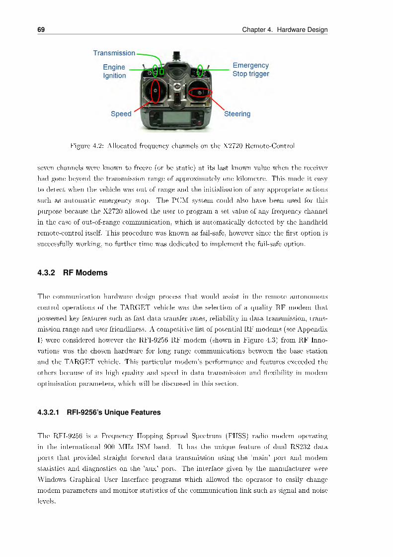
69 Chapter 4. Hardware Design
Figure 4.2: Allocated frequency channels on the X2720 Remote-Control
seven channels were known to freeze (or be static) at its last known value when the receiver
had gone beyond the transmission range of approximately one kilometre. This made it easy
to detect when the vehicle was out of range and the initialisation of any appropriate actions
such as automatic emergency stop. The PCM system could also have been used for this
purpose because the X2720 allowed the user to program a set value of any frequency channel
in the case of out-of-range communication, which is automatically detected by the handheld
remote-control itself. This procedure was known as fail-safe, however since the rst option is
successfully working, no further time was dedicated to implement the fail-safe option.
4.3.2 RF Modems
The communication hardware design process that would assist in the remote autonomous
control operations of the TARGET vehicle was the selection of a quality RF modem that
possessed key features such as fast data transfer rates, reliability in data transmission, trans-
mission range and user friendliness. A competitive list of potential RF modems (see Appendix
I) were considered however the RFI-9256 RF modem (shown in Figure 4.3) from RF Inno-
vations was the chosen hardware for long range communications between the base station
and the TARGET vehicle. This particular modem's performance and features exceeded the
others because of its high quality and speed in data transmission and exibility in modem
optimisation parameters, which will be discussed in this section.
4.3.2.1 RFI-9256’s Unique Features
The RFI-9256 is a Frequency Hopping Spread Spectrum (FHSS) radio modem operating
in the international 900 MHz ISM band. It has the unique feature of dual RS232 data
ports that provided straight forward data transmission using the 'main' port and modem
statistics and diagnostics on the 'aux' port. The interface given by the manufacturer were
Windows Graphical User Interface programs which allowed the operator to easily change
modem parameters and monitor statistics of the communication link such as signal and noise
levels.

4.3. Communication Hardware 70
Figure 4.3: The RFI-9256 RF Modem (RF Innovations Pty Ltd, 2006)
The way that the RFI-9256 handled its data transmission showed that the established com-
munication link was robust. Contributing to this was the large 32-bit Cyclic Redundancy
Checking (CRC) error checking operation (most other modems on the market have only
16-bit CRC). In addition to the RFI-9256's CRC, was the Forward Error Checking (FEC)
operation which was also not present in other industrial modems. This feature detected if
there were any errors in a packet transmission that were amendable and would automatically
make the appropriate adjustments.
4.3.2.2 Protocol Operations
Protocol operations are modes that determine how the serial port data is interpreted and
converted in to data packets for transmission over the air (RF Innovations Pty Ltd, 2006).
The RFI-9256 supported four dierent protocol operations: Point-to-Point, Broadcast, Hayes
Dial-Up and SCADA. The project's application only involved two modems at two locations
which meant the Broadcast and SCADA protocols were not applicable. Although the Point-
to-point protocol could have been used, Hayes Dial-up was chosen because more exibility and
support was given regarding that protocol. In Hayes Dial-Up there exists a 'master' modem
which is the one that sets the parameters of any other modem that it connects to. The master
modem is also responsible for synchronising with the remote or 'slave' modem that it wishes
to connect to. Hence the most appropriate location to place the master modem was at the
base station computer where the operator had easy access to. The conguration of the master
and slave modem in a Hayes Dial-Up network was congured such that:
• They both had the same hopping pattern, network address, and security code
• The master and slave had dierent local addresses
• Both the master and slave had the Hayes Dial-Up protocol selected on the their main/aux
serial port

71 Chapter 4. Hardware Design
• The point-to-point destination address on the slave is set to the master's local address,
while the destination address on the master is set to the slave's local address (RF
Innovations Pty Ltd, 2006).
An example of such congurations is shown in Figure 4.4.
Figure 4.4: Basic Hayes Dial-Up Network conguration (RF Innovations Pty Ltd, 2006)
4.3.2.3 Overview of the RFI-9256’s Operation
The operation of the RFI-9256 modem is summarised in Figure 4.5. This shows the data
path of information being transmitted from one end to another in full duplex operation. The
transmission of one frame of data is divided into two packets where one carries the payload
of the master modem and the other carries the payload from the slave modem.
Figure 4.5: Data path operation of the RFI-9256 (RF Innovations Pty Ltd, 2006)
It is inevitable to have latency in any wireless communication system. There are three types
of latencies that the RFI-9256 modem inicts. The rst is the Serialisation Delay which is
caused by the time taken for the incoming RS232 bit stream to be converted back into bytes.
The second type of latency is called Framing Delays, which are caused when data packets
arrive at the start or end of frame times. Packets arriving half way through a frame will have
to wait until the start of the next frame is ready. The maximum latency caused by framing
4.3. Communication Hardware 72
delays is equal to the frame time which is the default, but user selectable, 20ms. Finally,
the third type of latency is due to the quality of the wireless communication link. A bad
link, usually due to RF interference, will cause the modem to resend any corrupted packets.
This is known as packet retries. The more retries that are required to send a packet through,
the greater the latency time. The overall latency can be somewhat minimised by setting the
appropriate conguration parameters as discussed in the next sub-section.
4.3.2.4 RFI-9256 Configuration Parameters
Transmit Power
The transmit power of the RFI-9256 (device only) can range from +0dBm to +30dBm. Cables
introduced loss and the antenna introduced gain, hence the transmitting power of the modem
was congured such that the power at the antenna's locations was as close to +30dBm as
possible.
Frame Time
The frame time is the amount of time that the RFI-9256 will spend on each channel in the
hopping pattern. A decrease in frame time caused a decrease in latency but also decreased
the data throughput and vice versa. Hence the frame time was set to a reasonable 20ms to
optimise data throughput while not causing too much latency in data transmission.
Directional Bias
The directional bias setting was enabled so that it allowed the user to conduct the majority
of data ow between the master and slave modem. This was achieved by increasing the data
packet sizes of either the master or slave modem. Having this feature was benecial to project
as most transmitted data would ow from the TARGET vehicle to the base station.
Packet Retries
Packet retries is the procedure of resending data packets that were detected lost or corrupted
during the rst attempt. The maximum number of retries per frame can be congured between
zero and two hundred and fty ve. Setting this number low caused the communication link
to be vulnerable to interference but would minimise latency. A high number of retries would
increase the robustness of the link however it would also increase signicant latency in the
presence of interference. The environment that the vehicle was tested in showed moderate
interference (+115dBm) as shown by the modem statistics menu, hence the number of packet
retries was set in the mid-range (200 retries).
RSSI Trigger Level
The Receive Signal Strength Indication (RSSI) trigger level sets the lowest RSSI that the
modem is to attempt to acquire data (RF Innovations Pty Ltd, 2006). In a noisy environment,

73 Chapter 4. Hardware Design
the background noise may rise above the modem's sensitivity of -108dBm. In this case the
RSSI trigger level must be set higher to allow the master and slave modems to communicate.
However, setting the RSSI trigger level too high will articially deafen the modem. For
previous testing, the the RSSI trigger level was set to -108dBm.
4.4 Steering Actuation
The steering actuation system of the TARGET project has the role of providing full steering
control to the vehicle platform. The steering actuation system can be separated into three
subsections, covering the steering motor, mounting arrangement and measurement of the
steering angle. The design of the overall steering system used in the TARGET project has
been based on the steering actuation systems discussed in Section 3.1. These systems, as well
as the steering actuation system used in the TARGET project, consist of an electric motor
coupled to the steering column of the vehicle. A chain and two sprockets have been used to
provide the linkage between the electric motor and steering column, and are shown in Figure
4.8.
4.4.1 Steering Motor
A motor was chosen to actuate the steering of the TARGET vehicle based on two design
considerations. These design considerations were the torque required to turn the steering
wheel and the speed at which the steering wheel needed to be turned. Measurements were
taken of the torque required to steer the vehicle when it was stationary, as this is where the
maximum amount of torque is required to turn the steering wheel. It was found that an
approximate torque of 5 Nm was required to steer the vehicle.
Selection of an electric motor to drive the steering was based on the measured torque as well
as a design factor. A design factor of 4 was chosen as this is regarded a critical design factor,
and the steering system of the vehicle is a critical system where errors could result in serious
safety issues. Using a design factor of 4 implied that an electric motor capable of providing a
20 Nm of torque was required to actuate the steering of the vehicle.
Selection of the speed of the motor was done by measuring how fast a driver needed to turn
the wheel to complete a track similar to that described in Chapter 2. The maximum speed
required to turn the steering wheel was found to be approximately 1 rev/s.
The motor selected for use in the steering actuation system was the 'Bison 348 Series PMDC'
gearmotor (shown in Figure 4.6). This motor is capable of providing 17 Nm of continuous
torque and can approach torques of up to 23 Nm for a limited amount of time. Averaging the
intermittent and continuous value yields an average torque provided of 20 Nm. This torque
corresponds to a design factor of 4 relative to the measured torque of 5 Nm. The speed of
the motor is 64 rev/min which is slightly greater than the required speed of 1 rev/s. Control

4.4. Steering Actuation 74
Figure 4.6: Bisongear 348 Series PMDC Gearmotor (Bison Gear & Engineering Corp, 2007)
of the motor is covered in Section 6.3.1 and the electrical connections are covered in Section
4.8.7. Some of the main features of the 'Bison 348 Series PMDC' gearmotor are listed in the
following points:
• Maximum current draw of 14 A
• Continuous output torque of 17 Nm
• Intermittent output torque of 23 Nm
• Shaft rotational speed of 64 rev/min
• Gear ratio of 28:1
4.4.2 Mounting Arrangement
Mounting of the steering system needed to be implemented in a fashion that did not interfere
with the regular operation of the vehicle as outlined in Chapter 2. An extension goal of the
TARGET project was to approve the vehicle to be road legal (see Chapter 2). To make the
vehicle road legal, the steering system needed to be mounted so that it was in compliance
with requirements set by Transport SA regarding safety of the vehicle. Transport SA's only
requirement for the steering system, was that it needed be positioned behind the steering
column, so that in the event of a collision, the existing safety collapsing mechanism of the
steering column was not interfered with.
Considerations were also made in deciding the mounting position of the steering system with
regard to the position of the linkage system between the gearmotor and the steering column.
The section of the steering column shown in Figure 4.7 that is highlighted in red was chosen
to be the linkage point between the gearmotor and the steering. This was considered to be a
suitable linkage position as it is a large and easily accessible area of the steering column.

75 Chapter 4. Hardware Design
Figure 4.7: Steering column of TARGET vehicle
The mounting position of the motor was chosen to be directly behind the section of the
steering column, shown by the yellow area in Figure 4.7. This position allows a regular driver
of the vehicle to place their feet either side of the actuation system where they would normally
be placed without interference. The accelerator and brake pedals are also not interfered with
by mounting the actuation system in this location.
Selection of the linkage system between the gearmotor and the steering column was largely
based on Section 3.1. From the three linkage systems found in Section 3.1, which were gears,
belt and chain, a chain was found to be the most suitable. This is due to the relative simplicity
of the chain and sprocket system, where the chain can easily be removed from the system when
needed by using a chain breaker. The other linkage methods discussed in section 3.1 would
require the steering column to be dismantled to remove the linkage system.
The sprockets used on the steering column and on the motor shaft have a gear ratio of 1:1,
with both sprockets having 17 teeth. This ratio was chosen as the Bison gearmotor already
had a gear ratio of 28:1, and supplied the required level of torque at the desired shaft speed,
so no further gear reduction was necessary. The installed chain is shown in Figure 3.3 (b).
To mount the gearmotor, a bracket and plate were used as shown in Figure 4.8. The bracket
is designed to hold the output shaft of the gearmotor parallel to the steering column so that
the sprockets are in the same plane. The bracket may also be moved backward and forward to
tighten or loosen the chain and can also be completely removed by removing bolts that hold
the bracket in place. The plate mounted on the oor of the vehicle provides extra support to
the oor of the vehicle so that it does not buckle when subjected to indirect loads applied to
it from the gearmotor.

4.4. Steering Actuation 76
(a) Steering system location
(b) Motor and steering column chain linkage
Figure 4.8: TARGET Vehicle steering actuation system

77 Chapter 4. Hardware Design
Figure 4.9: Steering potentiometer
4.4.3 Steering Angle Measurement
Feedback on the steering wheel angle was also required for the control of the vehicle's steering
(see Section 6.3.1). Due to the high accuracy of the on-board computers analogue inputs (see
Section 6.1.1), and also for simplicity of the system a potentiometer was used to generate
feedback for the steering position by coupling it to the steering column using a toothed belt
and pulleys (shown in Figure 4.9).
The potentiometer used was an 'ETI Systems, 10 Turn Wire wound Precision Potentiometer'
rated at 1 kΩ. Although the steering column only needs 3.5 revolutions to travel from lock
to lock, a 10 turn potentiometer was used as they are easily accessible. A gear ratio was used
on the pulleys connecting the steering column to the potentiometer to utilize a greater range
of the potentiometer. The gear ratio was 25 teeth on the steering column to 15 teeth on the
potentiometer. This gear ratio resulted in the potentiometer utilizing 5.8 revolutions of the
available 10 revolutions, producing a high quality signal output to the onboard computer.
Coupling the potentiometer directly to the steering column rather than the motor resulted in
the potentiometer only being required to be calibrated once, rather than every time the motor
is disconnected from the steering column. Another advantage of having the potentiometer
connected directly to the steering column is that in the unlikely event of the motor becoming
uncoupled from the steering column, the potentiometer reading will still be correct as it is
not dependent on the motor being connected.
To ensure the potentiometer shaft was not subjected to excessive force, a exible coupling
was installed into the system as shown in Figure 4.9. This was done as excessive force on
the potentiometer shaft can cause the potentiometer to ware, and over time fail. The exible
coupling is able to deform whilst still allowing the shaft of the potentiometer to rotate.

4.5. Throttle Actuation 78
4.5 Throttle Actuation
The throttle actuation system of the TARGET project has the objective of providing full
throttle control of the vehicle platform whilst allowing for a regular driver to operate the
throttle. This system has been implemented by using an actuator from a cruise control
system to actuate the throttle valve of the vehicle. The actuation is done in a similar manner
to how the cable connected to the foot pedal of the vehicle moves the throttle valve.
4.5.1 Vacuum Actuator Mounting
The actuator used from the cruise control system is a vacuum actuator. This actuator is
connected to the vacuum hose of the vehicle, and by controlling a series of valves with solenoids
a diaphragm inside the actuator can be moved in and out. This diaphragm is then connected
to a cable, which is connected to the throttle valve of the vehicle. The connection with the
vacuum hose is illistrated in Figure 4.10.
Figure 4.10: Instructions describing how to connect the actuator to the vehicle vacuum line(Auscruise By Autron, 2007)
The actuator itself was then mounted to the engine bay of the vehicle as shown in Figure 4.11
(a), with the cable connected to the throttle valve as shown in Figure 4.11 (b).
4.5.2 Vacuum Actuator Control
Control of the vacuum actuator is achieved by operating four pins, which control three
solenoids inside the actuator. The pins are usually connected to the electronics designed
by the cruise control manufacturer. However, in order to integrate the actuator for the re-
quired purpose of the TARGET project, the standard manufactures electronics were not used

79 Chapter 4. Hardware Design
(a) Vacuum actuator mounted inside the engine bay
(b) Throttle valve connection
Figure 4.11: TARGET throttle actuation system
and instead the actuator was controlled by digital lines from the on-board computer system
(see Section 6.1.4.2). The pins of the vacuum actuator are classied as follows:
Pin 1: Vacuum inlet solenoid. Activating this pin opens a valve that allows the vacuum line
of the vehicle to pull the diaphragm of the vacuum actuator in.
Pin 2: Control dump solenoid. Activating this pin allows a free ow of air through the
actuator. Activating pin 1 has no eect when pin 2 is activated.
Pin 3: +12 V supply to the actuator.
Pin 4: Safety dump solenoid. Activating this pin causes the actuator to completely release
the throttle in case of an emergency.
Activating the safety dump solenoid needs to be done from the capacitive brake sensor (see
Section 4.8.2) and the dragon safety system (see Section 8.1.2). Therefore electronics were
made so that when either of these signals were activated the throttle was released.
4.6 Brake Actuation
The brake actuation system of the TARGET project has the purpose of providing full brake
control of the vehicle platform. The brake system is designed to provide a controlled means

4.6. Brake Actuation 80
Figure 4.12: A brief overview showing the sequential operation of the primary brake actuationsystem
of decceleration of the TARGET vehicle during autonomous and remote controlled operation.
Design of the brake system has also taken into consideration a secondary brake system to be
activated in the event of an emergency. Achieving successful implementation of these systems
was also carried out with regard to the extension goal (see Section 2) to not interfere with
the normal operations of the TARGET vehicle.
4.6.1 Primary Brake Actuation System
The primary brake actuation system of the TARGET vehicle has been implemented by using a
linear actuator, linked to the brake pedal of the vehicle with a cable, to provide a pulling force
on the brake pedal. This brake actuation system design was used because its implementation
had very low interference with the normal operation of the brake pedal.
The ow of the primary brake actuation system for the TARGET vehicle si illustrated in
Figure 4.12. The system consists of an amplier, linear actuator, pressure transducer, brake
cable and brake pedal. Each of these components will be further discussed in Sections 4.6.1.1
to 4.6.1.4.
4.6.1.1 Amplifier
The TARGET vehicle primary brake actuation system is controlled by the on-board computer
through the Roboteq AX1500 Amplier (see Section 4.8.7). With reference to Figure 4.12,
the amplier allows the on-board computer to position control the brake pedal through the
linkage with the linear actuator, and achieve vehicle deceleration.
4.6.1.2 Linear Actuator
A linear actuator was chosen for use in the primary brake actuation system of the TARGET
vehicle based on two design considerations. These design considerations include the force
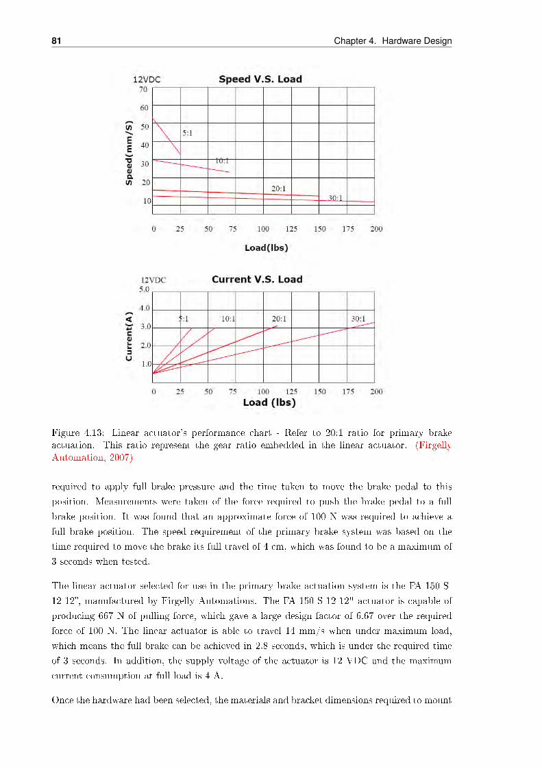
81 Chapter 4. Hardware Design
Figure 4.13: Linear actuator's performance chart - Refer to 20:1 ratio for primary brakeactuation. This ratio represent the gear ratio embedded in the linear actuator. (FirgellyAutomation, 2007)
required to apply full brake pressure and the time taken to move the brake pedal to this
position. Measurements were taken of the force required to push the brake pedal to a full
brake position. It was found that an approximate force of 100 N was required to achieve a
full brake position. The speed requirement of the primary brake system was based on the
time required to move the brake its full travel of 4 cm, which was found to be a maximum of
3 seconds when tested.
The linear actuator selected for use in the primary brake actuation system is the FA-150-S-
12-12, manufactured by Firgelly Automations. The FA-150-S-12-12" actuator is capable of
producing 667 N of pulling force, which gave a large design factor of 6.67 over the required
force of 100 N. The linear actuator is able to travel 14 mm/s when under maximum load,
which means the full brake can be achieved in 2.8 seconds, which is under the required time
of 3 seconds. In addition, the supply voltage of the actuator is 12 VDC and the maximum
current consumption at full load is 4 A.
Once the hardware had been selected, the materials and bracket dimensions required to mount

4.6. Brake Actuation 82
Table 4.1: Comparison table between the required and actual performance of the linear actu-ator
Description Required Performance Actual Performance
Pulling Force 100 N 667 N
Speed 13.3 mm/s 14 mm/s
Figure 4.14: The TARGET vehicle's brake and transmission actuator assembly
the hardware were selected. After consultation with both supervisors and an engineering
workshop assistant, the linear actuator was installed inside the TARGET vehicle as shown in
the Figure 4.14. The current installation was set up was to maintain an easy access to the
linear actuator to simplify maintenance and inspection processes.
The mounting brackets consist of four major components (Refer to Figure 4.14): the alu-
minum plate, U-shaped bracket, squared-blocked bracket, and the L-shaped bracket. An
aluminum plate with a thickness of 3mm was selected as a platform to mount the linear
actuator. Aluminum was used to mount the actuators for aesthetic purposes, whilst it still
providing sucient strength. The U-shaped and squared-block brackets were implemented
for the purpose of preventing the linear actuator from lateral and translational motions. The
L-shaped bracket was installed to hold the outer casing of brake cable in place.
4.6.1.3 Pressure Transducer
The pressure transducer was implemented into the brake pressure line of the braking system
to provide a feedback signal from the brake to the on-board computer (Refer to Figure 4.12).
The pressure transducer selected was the GE Druck - PTX 1400 (Refer to Figure 4.15) man-
ufactured by General Electric. The GE Druck - PTX 1400 was selected based on the pressure
range in the brake lines, given by the vehicle manual, which are listed in the Table 4.2. The

83 Chapter 4. Hardware Design
Figure 4.15: Pressure transducer GE Druck - PTX 1400
Table 4.2: Braking Conditions and the expected pressure range - Mitsubishi Express 1994Braking Condition Pressure Range Impact to the vehicle
Low 0 - 300 Psi None
Moderate 300 - 400 Psi Moderate deceleration
High 800 - 900 Psi Fast deceleration
Extreme 1200 - 1500 Psi All wheels locked up(Emergency Braking)
maximum amount of breaking pressure required to lock the brakes is approximately 60bar.
The range of the pressure transducer was chosen to be 0 - 60 bar (0 - 870.23 psi) for this
reason. This places the transducer in the fast deceleration pressure range of Table 4.2. It
ensures dangerously high pressures are not obtained and the wheels do not lock.
It is necessary to convert the output current into an output voltage that it can be interpreted
by the analogue card, discussed in Section 4.2.2.2 of the on-board computer (i.e. receiving
0-5 V, not 4-20 mA). Using Ohm's Law, it was calculated that a 270Ω resistor will need to be
added to the pressure transducer to produce the desired output voltage. The circuit diagram
used to convert the current output to a voltage output is shown in Figure 4.16.
The pressure transducer was installed inside the vehicle, close to master cylinder, as illustrated
in Figure 4.17. The pressure transducer was installed inside the vehicle to prevent exposure
to excessive dust, dirt, and moisture.
Installation of the pressure transducer required modications to be made to the vehicle brake
pressure line. The components required for the installation were (Refer to Figure 4.18 (a) from
the top left): 10/1MM DPS 3-WAY Connector, 1/2x20 - 3/8x24 Adapter, 3/16 10x1MM Tube
Nut, and 3/16-1/4 Straight PI. These components were then installed as shown in Figure 4.18
(b).
4.6.1.4 Brake Cable and Brake Pedal
The brake cable was used to enable the linear actuator to transmit the mechanical pulling
force from the actuator to the vehicle brake pedal. With reference to Figure 4.14, the L-shaped

4.6. Brake Actuation 84
Figure 4.16: Modied circuit diagram of the pressure transducer to generate the desiredvoltage output
Figure 4.17: Mounting arrangement for the pressure transducer of the TARGET vehicle

85 Chapter 4. Hardware Design
(a) Individual components
(b) Assembled components
Figure 4.18: Pictorial representations of individual components and the assembled componentfor brake line modication purpose
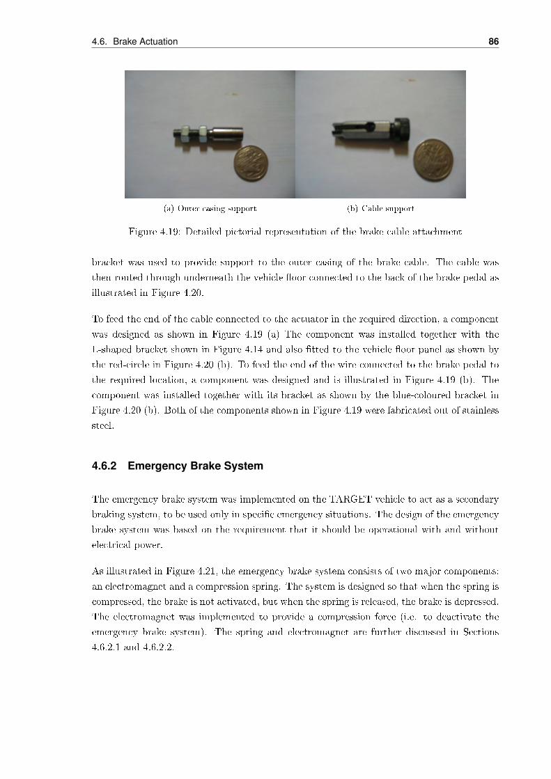
4.6. Brake Actuation 86
(a) Outer casing support (b) Cable support
Figure 4.19: Detailed pictorial representation of the brake cable attachment
bracket was used to provide support to the outer casing of the brake cable. The cable was
then routed through underneath the vehicle oor connected to the back of the brake pedal as
illustrated in Figure 4.20.
To feed the end of the cable connected to the actuator in the required direction, a component
was designed as shown in Figure 4.19 (a) The component was installed together with the
L-shaped bracket shown in Figure 4.14 and also tted to the vehicle oor panel as shown by
the red-circle in Figure 4.20 (b). To feed the end of the wire connected to the brake pedal to
the required location, a component was designed and is illustrated in Figure 4.19 (b). The
component was installed together with its bracket as shown by the blue-coloured bracket in
Figure 4.20 (b). Both of the components shown in Figure 4.19 were fabricated out of stainless
steel.
4.6.2 Emergency Brake System
The emergency brake system was implemented on the TARGET vehicle to act as a secondary
braking system, to be used only in specic emergency situations. The design of the emergency
brake system was based on the requirement that it should be operational with and without
electrical power.
As illustrated in Figure 4.21, the emergency brake system consists of two major components:
an electromagnet and a compression spring. The system is designed so that when the spring is
compressed, the brake is not activated, but when the spring is released, the brake is depressed.
The electromagnet was implemented to provide a compression force (i.e. to deactivate the
emergency brake system). The spring and electromagnet are further discussed in Sections
4.6.2.1 and 4.6.2.2.

87 Chapter 4. Hardware Design
(a) Brake cable and brake pedal link
(b) Brake cable and brake pedal Link - Side view
Figure 4.20: Brake pedal and brake cable link of the TARGET vehicle

4.6. Brake Actuation 88
Figure 4.21: Emergency Brake System of the TARGET vehicle
Table 4.3: Specication for the electromagnetMagnet Armature Size 65 mm
Holding Force 1300 N
Voltage Supply 12 VDC
Power Consumption 9.8 Watts
4.6.2.1 Electromagnet
The electromagnet was selected based on its holding force. The electromagnet was required
to sustain more than 100 N of force (i.e. more than required to operate the brake pedal of
the TARGET vehicle). The electromagnet used was a 65 MM 12VDC holding electromagnet,
manufactured by Magnet - Schultz Ltd. The specications for the magnet are listed in Table
4.3.
4.6.2.2 Compressional Spring
The compression spring was selected based on the braking pressure listed in Table 4.2. It was
selected so that during the activation of the emergency brake, the braking pressure will not
be too great (i.e. greater than 900 Psi). This is to prevent the wheels from locking up.
The calculations for the required spring characteristics was done by using the amount of force
required to produce the desired brake pressure combined with the desired deformation of the

89 Chapter 4. Hardware Design
Table 4.4: Specication for the compressional springForce 100N
Deformation 55mm
Spring Constant 1.81× 10³N/m
Length 103mm
Figure 4.22: Transmission actuation block diagram
spring (F = kx). The pressure reading was obtained from the installed pressure transducer
using a multimeter, whilst applying the desired force to the vehicle brake pedal with the
assistance of a digital force gauge. The selected spring characteristics are listed in Table 4.4.
4.7 Transmission Actuation
The transmission actuation was implemented to allow the on-board computer to change gears
during autonomous and remote controlled operation. The system was implemented using a
linear actuator linked to transmission lever. A block diagram of the transmission actuation
operation is illustrated in Figure 4.22.
In order to actuate the transmission, modications were made to the vehicle's transmission
lever. To move the transmission lever, an un-lock button is required to release the transmission
lever lock. An additional lever was attached to the unlock button in order for electronics
actuation to take place. Figures 4.23 (a) and (b) show the manufactured lever mechanism
(highlighted by the red-coloured circles). Figure 4.23 (a) also shows the modications made
to the transmission lever to allow for the linkage between the actuator and transmission
(highlighted by the blue-colored circle). The linkage between the transmission lever and
linear actuator is shown in Figure 4.24. The mechanical linkage was fabricated so that the
length of the linkage could be adjusted.
The transmission actuation is activated by the on-board computer. The computer will ac-
tivates a series of relays to enable the actuator to be moved forwards, backwards or held in
place. A solenoid has been used to depress the manufactured lever to unlock the transmission
lever. This solenoid automatically depresses the manufactured lever whenever the actuator
moves to unlock the transmission. As a result, gear shifting operation is achieved. In Figure

4.7. Transmission Actuation 90
(a) Transmission Lever - Side view (b) Transmission Lever - Front view
Figure 4.23: Modied gear transmission lever of the TARGET vehicle. Mechanical lever isindicated by the red circle in Subgure (a) and (b), modication to enable linkage betweenthe linear actuator and transmission lever is indicated by the blue circle in Subgure (a)
Figure 4.24: Linkage between transmission lever and actuator
4.22, it should be noted that the feedback signals were acquired from the gear position indi-
cator of the vehicle. The feedback allows the on-board computer to determine the position of
the transmission lever.
In the following subsections the solenoid, linear actuator and gear position indicators are
discussed in further detail.
4.7.1 Solenoid
The solenoid was implemented with the intention of locking and unlocking the vehicle's trans-
mission lever during autonomous and remote-controlled operations. This operation will then
permit the linear actuator to select between gears (i.e. Park, Drive, or Lower Gear). The

91 Chapter 4. Hardware Design
Figure 4.25: Solenoid installation to the vehicle transmission lever. Highlighted in red-coloured circle is the solenoid which connect the solenoid to the mechanical lever
selected solenoid, LR8814 (obtained from Jaycar Electronics), is commonly used to actuate
car central locking systems. It is capable of providing 3kg of pulling force against the required
force (of 1kg) to operate the lever-mechanism of the transmission lever. Furthermore, the life
time for this type of solenoid is 100,000 cycles. For the specied application the listed life
time was considered suitable. The installed solenoid is illustrated in Figure 4.25.
4.7.2 Linear Actuator
The linear actuator chosen for use in the transmission system is the FA-35-S-12-12, manufac-
tured by Firgelly Automations. The FA-35-S-12-12" actuator is capable of producing 16kg of
pulling force using 12 VDC . With reference to Figure 4.25, 3 Ampere of current will be used
by the linear actuator at its maximum load (35lbs≈16kgf). Furthermore, the linear actuatorwill be able to operate at a speed of approximately 25 mm/s at its maximum load.
For the actual applications of the transmission actuation system, the linear actuator will only
be required to provide a pull/push force of 25 Newtons (≈ 5.62lbs). Hence, it should be
noted that the actual performance required from the linear actuator is approximately 6 times
lower than the force that the linear actuator is capable of producing. This is due to the
design factor (as advised by our supervisor) which was taken into consideration during the
selection process. Hence, the comparison between the required performance and the actual
performance for the linear actuator can be summarized as shown in the Table 4.5. The values
in Table 4.5 were obtained from gear ratio 5:1 of Figure 4.13. The mounting arrangement for
the linear actuator is shown in Figure 4.14.

4.8. Electronics 92
Table 4.5: Comparison table between the expected performance of the linear actuator andthe selected specication of the actuator
Description Required Performance Actual Specication
Pulling Force 5.62 lbs 35 lbs
Speed 48 mm/s 25 mm/s
4.7.3 Gear Position Indicator
The gear position indicator is used to provide a positional feedback to the on-board computer
hence allowing the on-board computer to place the gear transmission lever to the desired
position. In order to assist the specied applications, minor modications were performed to
the dash-board of the TARGET vehicle (Refer to Figure 4.26). The cable was extended and
connected to an electronics board as indicate by the yellow-circle depicted in Figure 4.27.
4.8 Electronics
The electronics of the TARGET project are a separate system to the existing electronics
of the vehicle platform. There are some systems however that do overlap with the existing
electronics. This section will cover the major areas of the electronics, but will not go into
a high level of detail discussing the layout of the boards manufactured by the Mechanical
Engineering Workshop.
The electronic boards mounted inside the target vehicle are shown in Figure 4.28. Many of
the boards have multiple functions incorporated into their design, and therefore the labels in
Figure 4.28 refer to the main function of that particular board. The schematics of the boards
manufactured by the Mechanical Engineering Workshop can be found in Appendix H.
4.8.1 Power Electronics
To provide power to the additional systems installed in the vehicle, a secondary battery was
installed into the vehicle. This battery was added using a dual battery isolator (shown in
Figure 4.28), which directs the current from the alternator to charge both battery's when the
vehicle is running. When the vehicle is o the isolator allows the secondary battery to be
drained with no eect on the main battery.
The secondary battery is rated at 100 AHr. After testing the battery, it was found that the
systems running o of the battery took approximately 10 hours to completely run down the
battery.
Components used in the TARGET project require a range of dierent supply voltages. The
required supply voltages, and the components that require that supply voltage are listed as
follows:

93 Chapter 4. Hardware Design
(a) Dash board - Front End
(b) Dash board - Rear End
Figure 4.26: Modied dash-board of the TARGET vehicle for gear position signal acquisitions

4.8. Electronics 94
Figure 4.27: Close-up view of the TARGET electronics. Highlighted in yellow circle is thePCB board to accumulate gear position signal before connected to the TARGET computer

95 Chapter 4. Hardware Design
Figure 4.28: TARGET electronics
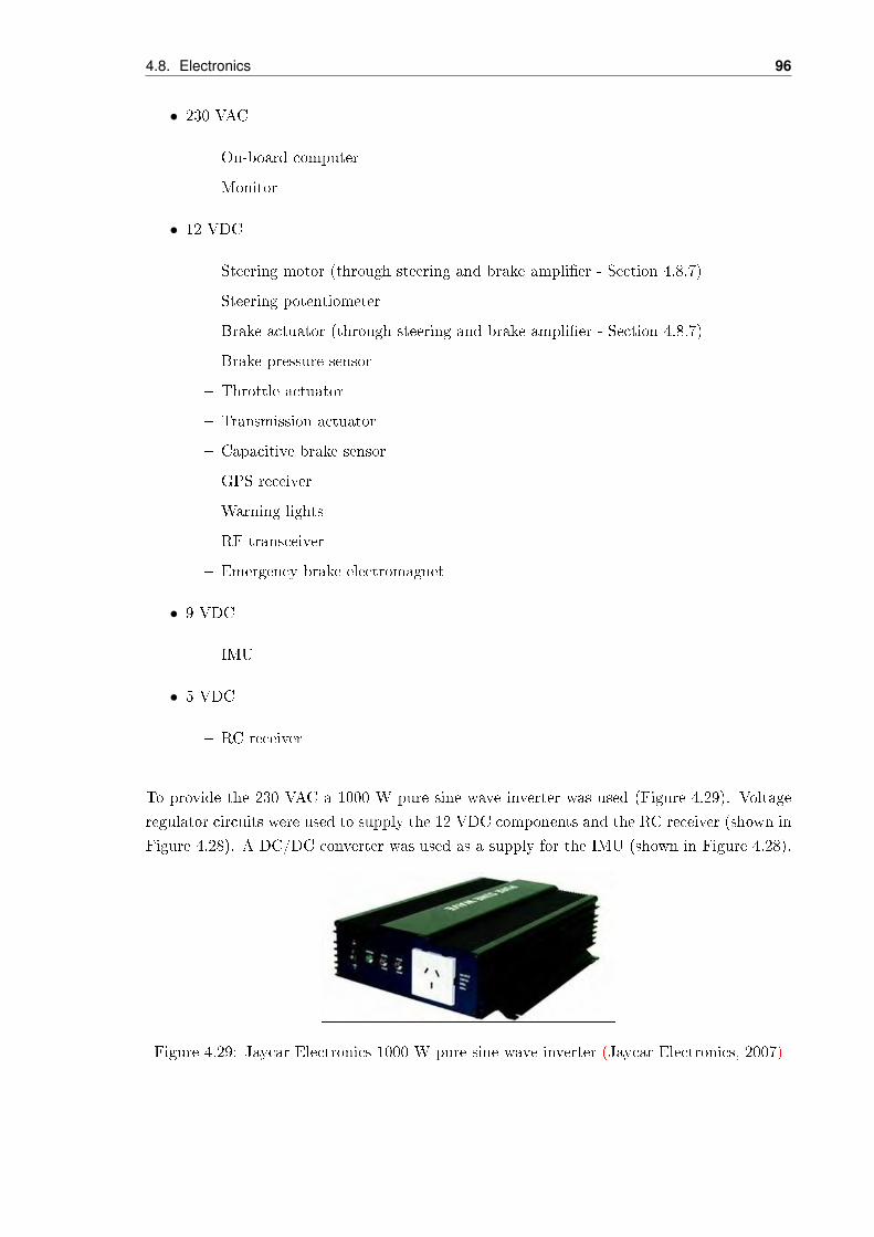
4.8. Electronics 96
• 230 VAC
On-board computer
Monitor
• 12 VDC
Steering motor (through steering and brake amplier - Section 4.8.7)
Steering potentiometer
Brake actuator (through steering and brake amplier - Section 4.8.7)
Brake pressure sensor
Throttle actuator
Transmission actuator
Capacitive brake sensor
GPS receiver
Warning lights
RF transceiver
Emergency brake electromagnet
• 9 VDC
IMU
• 5 VDC
RC receiver
To provide the 230 VAC a 1000 W pure sine wave inverter was used (Figure 4.29). Voltage
regulator circuits were used to supply the 12 VDC components and the RC receiver (shown in
Figure 4.28). A DC/DC converter was used as a supply for the IMU (shown in Figure 4.28).
Figure 4.29: Jaycar Electronics 1000 W pure sine wave inverter (Jaycar Electronics, 2007)
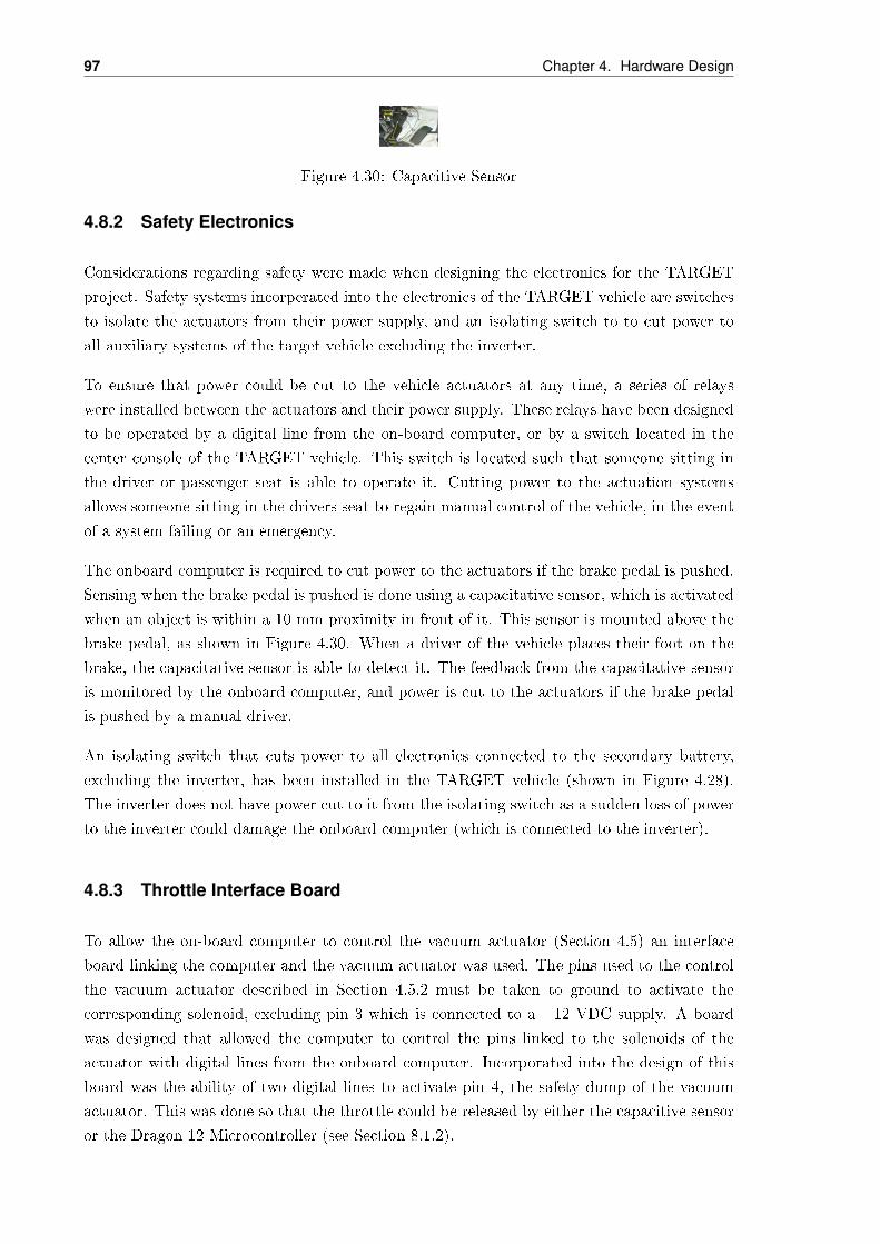
97 Chapter 4. Hardware Design
Figure 4.30: Capacitive Sensor
4.8.2 Safety Electronics
Considerations regarding safety were made when designing the electronics for the TARGET
project. Safety systems incorperated into the electronics of the TARGET vehicle are switches
to isolate the actuators from their power supply, and an isolating switch to to cut power to
all auxiliary systems of the target vehicle excluding the inverter.
To ensure that power could be cut to the vehicle actuators at any time, a series of relays
were installed between the actuators and their power supply. These relays have been designed
to be operated by a digital line from the on-board computer, or by a switch located in the
center console of the TARGET vehicle. This switch is located such that someone sitting in
the driver or passenger seat is able to operate it. Cutting power to the actuation systems
allows someone sitting in the drivers seat to regain manual control of the vehicle, in the event
of a system failing or an emergency.
The onboard computer is required to cut power to the actuators if the brake pedal is pushed.
Sensing when the brake pedal is pushed is done using a capacitative sensor, which is activated
when an object is within a 10 mm proximity in front of it. This sensor is mounted above the
brake pedal, as shown in Figure 4.30. When a driver of the vehicle places their foot on the
brake, the capacitative sensor is able to detect it. The feedback from the capacitative sensor
is monitored by the onboard computer, and power is cut to the actuators if the brake pedal
is pushed by a manual driver.
An isolating switch that cuts power to all electronics connected to the secondary battery,
excluding the inverter, has been installed in the TARGET vehicle (shown in Figure 4.28).
The inverter does not have power cut to it from the isolating switch as a sudden loss of power
to the inverter could damage the onboard computer (which is connected to the inverter).
4.8.3 Throttle Interface Board
To allow the on-board computer to control the vacuum actuator (Section 4.5) an interface
board linking the computer and the vacuum actuator was used. The pins used to the control
the vacuum actuator described in Section 4.5.2 must be taken to ground to activate the
corresponding solenoid, excluding pin 3 which is connected to a +12 VDC supply. A board
was designed that allowed the computer to control the pins linked to the solenoids of the
actuator with digital lines from the onboard computer. Incorporated into the design of this
board was the ability of two digital lines to activate pin 4, the safety dump of the vacuum
actuator. This was done so that the throttle could be released by either the capacitive sensor
or the Dragon 12 Microcontroller (see Section 8.1.2).

4.8. Electronics 98
4.8.4 Hall Effect Sensor Board
Digital feedback from the Hall eect sensor described in Section 5.4.3, was originally intended
to be interpreted by the digital cards of the on-board computer. However, the signal processing
required to interpret the feedback from the Hall eect sensor was using a large amount of CPU
processiong power, and resulted in CPU overloads. To avoid the possibility of a CPU overload,
it was decided to manufacture a board to convert the digital signal from the Hall eect sensor
to an analogue voltage output. This board was manufactured so that the output voltage
related to speed, and the relationship is dened in Equation 4.1.
speed = 78.4× voltage (4.1)
4.8.5 Tachometer Feedback Board
Feedback on the engine speed was required to control the throttle when the vehicle was in
park or neutral, as described in Section 6.3. To do this a board was made that provided an
analogue feedback to the on-board computer, by using the signal from the tachometer display
of the vehicle.
4.8.6 Ignition Board
Control of the ignition of the TARGET vehicle was a requirement of the TARGET project,
covered in Chapter 2. A board was made that was able to control the ignition from the
on-board computer. This board still allowed the vehicle to be started normally with a key.
To operate the ignition from the computer, the accessory electronics of the vehicle were still
required to be turned on with the vehicle key. Control of the ignition is covered in Section
??.
4.8.7 Steering and Brake Amplifier
A DC motor controller was required to convert commands from the on-board computer to
the required outputs to the steering motor (see Section 4.4.1) and brake actuator (see Section
??). The controller selected for use was the 'Roboteq AX1500' and is shown in Figure 4.31
(a). The features that suited the AX1500 to the TARGET project are listed as follows:
• 2 output channels
• 30 A maximum current output
• Serial (RS232), analogue or PWM command modes

99 Chapter 4. Hardware Design
• 12 - 40 V operation
• Up to 60 Hz operation speed
The 2 output channels of the AX1500 are shown in Figure 4.31 (b), where the 'motor 1'
output is connected to the steering motor and the 'motor 2' output is connected to the brake
actuator. The current output from the motor controller is far greater than required by the
steering motor or brake actuator. The maximum current required by the steering motor is
14 A, and a maximum current of 3 A is required for the brake actuator. Previous experience
with similar products inuenced the decision to purchase a controller with a greater current
capacity than required. This was done as problems had been experienced with previous
projects where the controller could not supply the current claimed by the manufacturer.
The AX1500 is capable of serial, analogue and PWM control. For the TARGET project
serial control was used. Serial control was chosen as it is very accurate, and easy to integrate
with the on-board computers serial board. Both the brake actuator and steering motor are
controlled through a single serial port. Commands to the controller are streamed at 50 Hz
which is the same rate as the motor control loops are run, as covered in Section 6.1.
In addition to the serial commands recievied from the on-board computer, the brake and
steering systems need to be controlled by the Dragon 12 microcontroller. To do this an
RS232 switching board was manufactured by the Mechanical Engineering Workshop (shown
in Figure 4.28). If a digital line connected to the RS232 switching board from the Dragon
12 microcontroller is set to high, commands to the Roboteq AX1500 are recieved from the
Dragon 12 microcontroller. If the digital line connected to the Dragon 12 microcontroller is
set to low the Roboteq AX1500 responds to commands sent from the on-board computer.
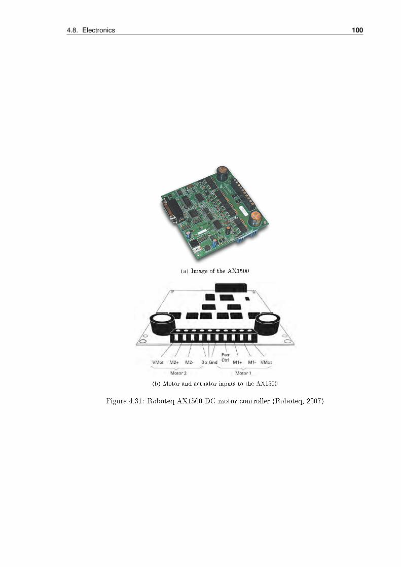
4.8. Electronics 100
(a) Image of the AX1500
(b) Motor and actuator inputs to the AX1500
Figure 4.31: Roboteq AX1500 DC motor controller (Roboteq, 2007)

Chapter 5
State Estimation and Measurement
Before commencing this Chapter, it must be noted that much of the terminology used here
is explained in the the State Estimation and Measurement Literature Review (Section 3.4).
Before reading on, the reader is strongly advised to return to this section of the Literature
Review to refresh their knowledge of the upcoming concepts.
This chapter focuses on the process of determining accurate estimates of the TARGET vehicle
states. As was discussed in the Literature Review, system states are often either not directly
available from sensors, or are corrupted with errors from these sensors. The purpose of the
state estimation process is to improve these corrupt measurements. The Kalman Filter, for
reasons outlined in the Literature Review, is selected as the primary tool for the state estima-
tion process. The Kalman Filter is implemented in software on the TARGET computer. It
runs in real-time and fuses the incoming sensor data into optimal state estimates. The main
focus of the state measurement and estimation section is on the suite of sensors onboard the
TARGET vehicle and the method of integrating them into the Kalman Filter. Section 5.1
describes the general structure and requirements of the Kalman Filter. Section 5.2 then dis-
cusses the required system states and Section 5.3 describes the system model. The individual
sensor inputs into the Kalman Filter are described in Section 5.4 where an overview is given
of each sensor, followed by the procedure for conguration of the device specically for use
in the TARGET vehicle. The Simulink subsystem which performs the sensor data decoding
is also described, and the method of integrating this decoded sensor data into the Kalman
Filter is discussed. Any tests which are required to complete the integration of the individual
sensors into the Kalman Filter are described, along with their results, at the end of each
sensor section. The focus is then brought back to a higher level by Section 5.5 which gives an
overview of the entire state estimation and measurement Simulink model. The performance of
this software in determining the vehicle states is then evaluated by a series of tests, described
and discussed in Section 5.6. Finally, some concluding remarks and recommendations for
future work are given in Section 5.7.
101
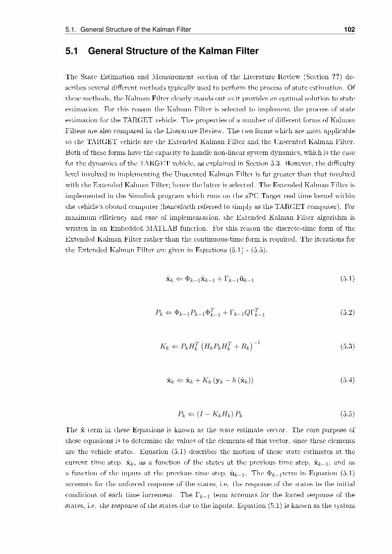
5.1. General Structure of the Kalman Filter 102
5.1 General Structure of the Kalman Filter
The State Estimation and Measurement section of the Literature Review (Section ??) de-
scribes several dierent methods typically used to perform the process of state estimation. Of
these methods, the Kalman Filter clearly stands out as it provides an optimal solution to state
estimation. For this reason the Kalman Filter is selected to implement the process of state
estimation for the TARGET vehicle. The properties of a number of dierent forms of Kalman
Filters are also compared in the Literature Review. The two forms which are most applicable
to the TARGET vehicle are the Extended Kalman Filter and the Unscented Kalman Filter.
Both of these forms have the capacity to handle non-linear system dynamics, which is the case
for the dynamics of the TARGET vehicle, as explained in Section 5.3. However, the diculty
level involved in implementing the Unscented Kalman Filter is far greater than that involved
with the Extended Kalman Filter; hence the latter is selected. The Extended Kalman Filter is
implemented in the Simulink program which runs on the xPC Target real-time kernel within
the vehicle's oboard computer (henceforth referred to simply as the TARGET computer). For
maximum eciency and ease of implementation, the Extended Kalman Filter algorithm is
written in an Embedded MATLAB function. For this reason the discrete-time form of the
Extended Kalman Filter rather than the continuous-time form is required. The iterations for
the Extended Kalman Filter are given in Equations (5.1) - (5.5).
xk ⇐ Φk−1xk−1 + Γk−1uk−1 (5.1)
Pk ⇐ Φk−1Pk−1ΦTk−1 + Γk−1QΓTk−1 (5.2)
Kk ⇐ PkHTk
(HkPkH
Tk +Rk
)−1(5.3)
xk ⇐ xk +Kk (yk − h (xk)) (5.4)
Pk ⇐ (I −KkHk)Pk (5.5)
The x term in these Equations is known as the state estimate vector. The core purpose of
these equations is to determine the values of the elements of this vector, since these elements
are the vehicle states. Equation (5.1) describes the motion of these state estimates at the
current time step, xk, as a function of the states at the previous time step, xk−1, and as
a function of the inputs at the previous time step, uk−1. The Φk−1term in Equation (5.1)
accounts for the unforced response of the states, i.e. the response of the states to the initial
conditions of each time increment. The Γk−1 term accounts for the forced response of the
states, i.e. the response of the states due to the inputs. Equation (5.1) is known as the system

103 Chapter 5. State Estimation and Measurement
model Equation and is the focus of Section 5.3. Note the use of the ⇐sign, rather than the
=sign in the equations. This species that the term on the left hand side for the equation
is to be replaced by the evaluation of the terms on the right hand side. This formality is
more accurate when describing the implementation of the Extended Kalman Filter iteration
in software.
Equation (5.2) provides a measure of the accuracy of the system model before any corrections
are made by the sensors in later Equations. For this reason Equation (5.2) is known as
the a-priori state covariance Equation and Pk, at this point in the Extended Kalman Filter
iteration, is known as the a-priori state covariance matrix. The a-priori state covariance matrix
is a function of the unfamiliar a-posteriori state covariance matrix, Pk−1, and process noise
covariance matrix, Q. The process noise covariance matrix describes the level of process noise
present in the system. In the case of the TARGET, this matrix describes the magnitude of the
eect of bumps in the road, gusts of wind and any other noise sources on the system states.
This process noise matrix is discussed in full detail in Section 5.3. The a-posteriori state
covariance matrix in Equation (5.2), Pk−1, provides a measure of the accuracy of the states
upon correction by the sensors. Note that in the rst iteration of the Extended Kalman Filter
Equations, the sensors have not had the chance to correct the states, therefore this matrix is
typically initialised to the identity matrix.
Equation (5.3) denes the instantaneous Kalman gain matrix, Kk, the vital component in
correcting the states with the sensor measurements (which is essentially the entire purpose
of the Kalman Filter). The unfamiliar terms in the calculation of the Kalman gain matrix
(Equation (5.3)) are the measurement matrix, Hk and the sensor noise covariance matrix,
Rk. The measurement matrix relates the states to the sensor measurements in the absence
of measurement noise and the sensor noise covariance matrix, Rk, describes this sensor noise,
which must be Gaussian if the lter is to function correctly. One or more Kalman gain
matrices are required for each individual sensor, implying that one or more measurement
matrices and one or more sensor noise covariance matrices are also required for each sensor.
The exact implementation of this Equation is covered in detail for each sensor in Section 5.4.
As has already been mentioned, the purpose of the Extended Kalman Filter is to correct
the state estimates with the available sensors. This is achieved using Equation (5.4) which
is known as the state update Equation and essentially calculates the dierence, or error,
between the sensor measurement vector, yk, and the transformed state estimates vector,
h (xk), multiplies it by the Kalman gain matrix and adds the resulting matrix to the current
state estimates. This correction stage is implemented for every sensor and is described in
greater detail in Section 5.4.
Finally, Equation (5.5) provides the method of updating the state a-posteriori covariance
matrix, Pk. As mentioned earlier, this matrix provides a measure of the accuracy of the
states after they have been corrected by the sensors.
Equation (5.1) must be implemented at a xed time period, T , and Equation (5.2) must
be implemented once for each time Equation (5.1) is executed. Equations (5.3) through

5.2. System States 104
(5.5) need only be implemented every time new information is available from a sensor. The
Kalman Filter Equations are relatively complex and the process is hard to visualise, therefore
a owchart has been created, given as Figure 5.1, to better visualise its iterative nature. This
ow chart only gives the EKF structure for two sensors, however it is clear how more sensors
would be incorporated.
5.2 System States
The states to be estimated by the Kalman Filter are dictated by the requirements of the
motion-execution controller, which is discussed in detail in Section 6.3, and the Autonomous
Guidance Controller, which is discussed in detail in Section 6.2. These controllers both require
accurate knowledge of certain vehicle states, so that the errors between the commanded state
value and the actual (or very accurate) state value may be minimised through actuation of
the TARGET vehicle. The Motion Execution Controller requires accurate knowledge of the
vehicle speed, v, and steering angle, φ; and the Autonomous Guidance Controller requires
accurate knowledge of the vehicle position, given in terms of Easting, E, and Northing, N ,
and the heading, θ. These states are dened visually in Figure (5.2).
The Kalman Filter requires that the states are placed in a vector, known as the state vector,
which is given as Equation (5.6)
x =
E
N
θ
v
a
φ
=
x1
x2
x3
x4
x5
x6
(5.6)
Note that the forward acceleration state, a, is also included in this vector although it is
not directly required by the vehicle controllers. This state is included as a means to relate
acceleration data, given by the inertial measurement unit, to the Kalman Filter. Every state
which is to be corrected by the Kalman Filter must be a function of a sensed quantity, which
clearly places requirements on the choice of sensors. Refer to Section 5.4.
In addition to the state vector, a vector of inputs is also required. The purpose of this vector
is to ensure that the system model, which is discussed in detail in Section 5.3, mimics the
true vehicle. The only requirement on the vector of inputs is that it must provide sucient
information to control the system model. The obvious solution is to set the system model
input states to be similar to the inputs which a driver typically uses to control a car, i.e. the
traction force at the four wheels generated by torque from the engine, the torque from the
brakes on the wheels and the steering angle of the front wheels (controlled by the accelerator
pedal, the brake pedal and the steering wheel respectively). It must be noted that within these
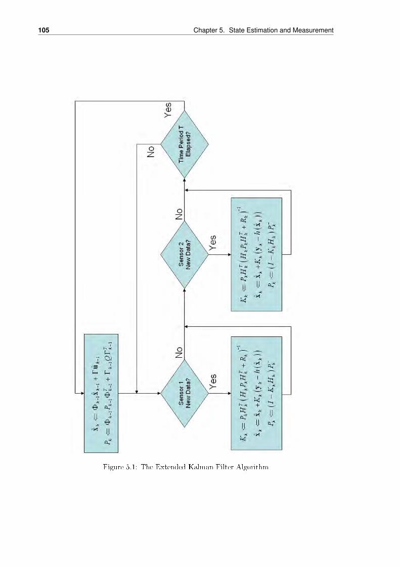
105 Chapter 5. State Estimation and Measurement
Figure 5.1: The Extended Kalman Filter Algorithm

5.3. System Model 106
Figure 5.2: A visual representation of the states to be determined
three inputs, the engine torque and the braking torque work cooperatively to eect a single
quantity, the vehicle forward acceleration. Therefore the engine torque and the braking torque
may be condensed to a single quantity, the vehicle forward acceleration, a. This acceleration
is dened as positive when the vehicle is accelerating forward and negative when the vehicle is
decelerating. The remaining input is the steering angle, φ, which does not require any further
simplication. Therefore the input vector is Equation (5.7).
u =
[a
φ
](5.7)
The system model, derived in Section 5.3, explains the process of relating the input vector to
the state vector Equation (5.6).
5.3 System Model
This section primarily focuses on deriving a mathematical model of the TARGET vehicle in a
form which is easily utilised in the Kalman Filter. When the model formulation is completed,
the model inputs, which ensure that the model states roughly match the true TARGET vehicle
states, are dened. The results of a number of tests, designed to determine the accuracy of
the system model in comparison to the true system, are presented and discussed in Section
9.5.1. Finally, Section 5.3.3 draws upon the results of the tests in Section 9.5.1 to determine
the process noise covariance matrix, which is required by the the Kalman Filter.
5.3.1 Derivation of the System Model
The model of the system consists of a matrix Equation which describes how the system
inputs, u, drive the system states, x, over time. Equation (5.8), also known as the system
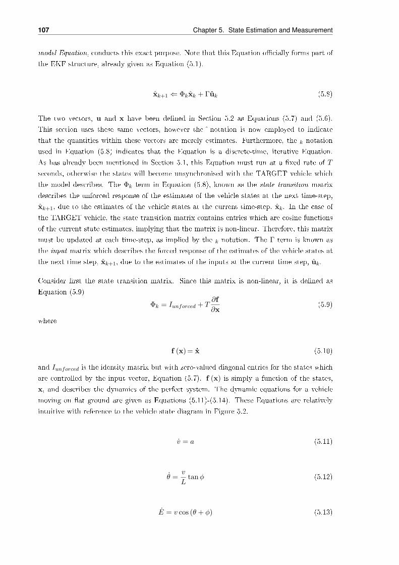
107 Chapter 5. State Estimation and Measurement
model Equation, conducts this exact purpose. Note that this Equation ocially forms part of
the EKF structure, already given as Equation (5.1).
xk+1 ⇐ Φkxk + Γuk (5.8)
The two vectors, u and x have been dened in Section 5.2 as Equations (5.7) and (5.6).
This section uses these same vectors, however the ˆ notation is now employed to indicate
that the quantities within these vectors are merely estimates. Furthermore, the k notation
used in Equation (5.8) indicates that the Equation is a discrete-time, iterative Equation.
As has already been mentioned in Section 5.1, this Equation must run at a xed rate of T
seconds, otherwise the states will become unsynchronised with the TARGET vehicle which
the model describes. The Φk term in Equation (5.8), known as the state transition matrix
describes the unforced response of the estimates of the vehicle states at the next time-step,
xk+1, due to the estimates of the vehicle states at the current time-step, xk. In the case of
the TARGET vehicle, the state transition matrix contains entries which are cosine functions
of the current state estimates, implying that the matrix is non-linear. Therefore, this matrix
must be updated at each time-step, as implied by the k notation. The Γ term is known as
the input matrix which describes the forced response of the estimates of the vehicle states at
the next time-step, xk+1, due to the estimates of the inputs at the current time-step, uk.
Consider rst the state transition matrix. Since this matrix is non-linear, it is dened as
Equation (5.9)
Φk = Iunforced + T∂f∂x
(5.9)
where
f (x) = x (5.10)
and Iunforced is the identity matrix but with zero-valued diagonal entries for the states which
are controlled by the input vector, Equation (5.7). f (x) is simply a function of the states,
x, and describes the dynamics of the perfect system. The dynamic equations for a vehicle
moving on at ground are given as Equations (5.11)-(5.14). These Equations are relatively
intuitive with reference to the vehicle state diagram in Figure 5.2.
v = a (5.11)
θ =v
Ltanφ (5.12)
E = v cos (θ + φ) (5.13)

5.3. System Model 108
N = v sin (θ + φ) (5.14)
Here L is the vehicle wheelbase length and all of the other variables are dened in detail in
Section (5.2). Equations (5.11)-(5.14) are put into the same form as Equation (5.10) to give
Equation (5.15).
E
N
θ
v
a
φ
=
v cos (θ + φ)v sin (θ + φ)
vL tanφa
00
(5.15)
This implies that
f (x) =
v cos (θ + φ)v sin (θ + φ)
vL tanφa
00
=
f1f2f3f4f5f6
(5.16)
All the vectors and matrices required by Equation (5.9) have now been dened. Firstly the
Jacobian term in Equation (5.9) is expanded out as Equations (5.17)
∂f (x)∂x
=
∂f1∂x1
∂f1∂x2
∂f1∂x3
∂f1∂x4
∂f1∂x5
∂f1∂x6
∂f2∂x1
∂f2∂x2
∂f2∂x3
∂f2∂x4
∂f2∂x5
∂f2∂x6
∂f3∂x1
∂f3∂x2
∂f3∂x3
∂f3∂x4
∂f3∂x5
∂f3∂x6
∂f4∂x1
∂f4∂x2
∂f4∂x3
∂f4∂x4
∂f4∂x5
∂f4∂x6
∂f5∂x1
∂f5∂x2
∂f5∂x3
∂f5∂x4
∂f5∂x5
∂f5∂x6
∂f6∂x1
∂f6∂x2
∂f6∂x3
∂f6∂x4
∂f6∂x5
∂f6∂x6
=
∂v cos(θ+φ)∂E
∂v cos(θ+φ)∂N
∂v cos(θ+φ)∂θ
∂v cos(θ+φ)∂v
∂v cos(θ+φ)∂a
∂v cos(θ+φ)∂φ
∂v sin(θ+φ)∂E
∂v sin(θ+φ)∂N
∂v sin(θ+φ)∂θ
∂v sin(θ+φ)∂v
∂v sin(θ+φ)∂a
∂v sin(θ+φ)∂φ
∂ vL
tanφ
∂E
∂ vL
tanφ
∂N
∂ vL
tanφ
∂θ
∂ vL
tanφ
∂v
∂ vL
tanφ
∂a
∂ vL
tanφ
∂xφ∂a∂E
∂a∂N
∂a∂θ
∂a∂v
∂a∂a
∂a∂φ
∂0∂E
∂0∂N
∂0∂θ
∂0∂v
∂0∂a
∂0∂φ
∂0∂E
∂0∂N
∂0∂θ
∂0∂v
∂0∂a
∂0∂φ
=
0 0 −v sin (θ + φ) cos (θ + φ) 0 −v sin (θ + φ)0 0 v cos (θ + φ) sin (θ + φ) 0 v cos (θ + φ)0 0 0 1
L tanφ 0 vL cos−2 φ
0 0 0 0 1 00 0 0 0 0 00 0 0 0 0 0
(5.17)
Now, implementation of Equation (5.9) on the TARGET computer requires Equation (5.17)

109 Chapter 5. State Estimation and Measurement
to be transformed into the discrete-time domain and Equation (5.17) to be written in terms
of the most accurate states available to the TARGET computer, i.e. the estimated states.
Therefore, Equation (5.9) becomes Equation (5.18).
Φk = Iunforced + T∂f∂x
]x=xk
=
1 0 0 0 0 00 1 0 0 0 00 0 1 0 0 00 0 0 1 0 00 0 0 0 0 00 0 0 0 0 0
+T
0 0 −vk sin(θk + φk
)cos(θk + φk
)0 −vk sin
(θk + φk
)0 0 vk cos
(θk + φk
)sin(θk + φk
)0 vk cos
(θk + φk
)0 0 0 1
L tan φk 0 vkL cos−2 φk
0 0 0 0 1 00 0 0 0 0 00 0 0 0 0 0
=
1 0 −T vk sin(θk + φk
)T cos
(θk + φk
)0 −T vk sin
(θk + φk
)0 1 T vk cos
(θk + φk
)T sin
(θk + φk
)0 T vk cos
(θk + φk
)0 0 1 T
L tan φk 0 T vkL cos−2 φk
0 0 0 1 T 00 0 0 0 0 00 0 0 0 0 0
(5.18)
Now that the state transition matrix, Φk has been fully dened (as Equation (5.18)), the
system model (Equation (5.8)) is complete, except for the input matrix, Γ, which remains
to be identied. The inputs to the system model are dened in Section 5.2 as the forward
acceleration and the steering angle. Consequently, the input matrix, Γ, is dened as Equation(5.19).
Γ =
0 00 00 00 01 00 1
(5.19)
This concludes the derivation of the system model. The model is given in complete form as
Equation (5.20).
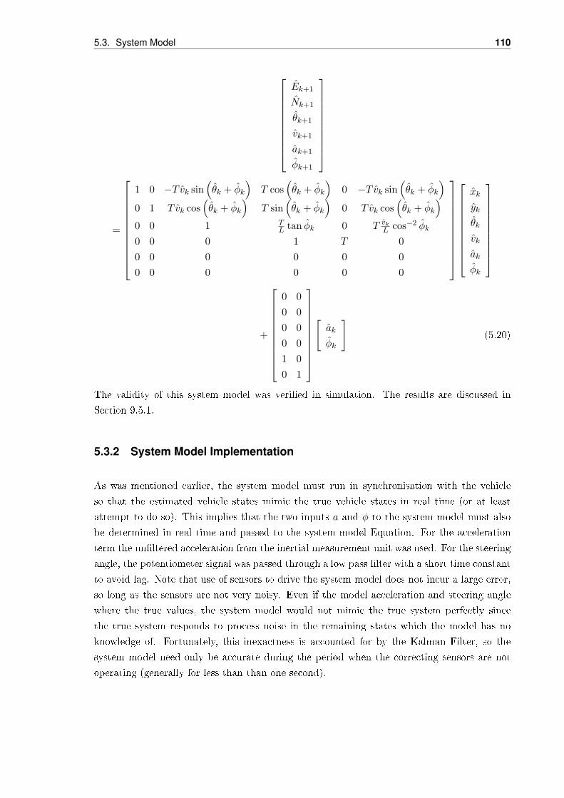
5.3. System Model 110
Ek+1
Nk+1
θk+1
vk+1
ak+1
φk+1
=
1 0 −T vk sin(θk + φk
)T cos
(θk + φk
)0 −T vk sin
(θk + φk
)0 1 T vk cos
(θk + φk
)T sin
(θk + φk
)0 T vk cos
(θk + φk
)0 0 1 T
L tan φk 0 T vkL cos−2 φk
0 0 0 1 T 00 0 0 0 0 00 0 0 0 0 0
xk
yk
θk
vk
ak
φk
+
0 00 00 00 01 00 1
[ak
φk
](5.20)
The validity of this system model was veried in simulation. The results are discussed in
Section 9.5.1.
5.3.2 System Model Implementation
As was mentioned earlier, the system model must run in synchronisation with the vehicle
so that the estimated vehicle states mimic the true vehicle states in real time (or at least
attempt to do so). This implies that the two inputs a and φ to the system model must also
be determined in real time and passed to the system model Equation. For the acceleration
term the unltered acceleration from the inertial measurement unit was used. For the steering
angle, the potentiometer signal was passed through a low pass lter with a short time constant
to avoid lag. Note that use of sensors to drive the system model does not incur a large error,
so long as the sensors are not very noisy. Even if the model acceleration and steering angle
where the true values, the system model would not mimic the true system perfectly since
the true system responds to process noise in the remaining states which the model has no
knowledge of. Fortunately, this inexactness is accounted for by the Kalman Filter, so the
system model need only be accurate during the period when the correcting sensors are not
operating (generally for less than than one second).

111 Chapter 5. State Estimation and Measurement
5.3.3 Derivation of the Process Noise Covariance Matrix
The process noise covariance matrix is dened as the matrix product of the process noise
vector, w, and its own transpose, as per Equation (5.21).
Q = wwT (5.21)
The process noise vector is dened as the standard deviation of each of the vehicle states, due
to physical disturbances (as opposed to sensor disturbances), from the perfect system model.
This vector is given by Equation(5.22).
w =
σE
σN
σθ
σv
σa
σφ
(5.22)
The tests to determine the values of each of these standard deviations are listed in Section
9.5.1. The process noise covariance matrix (Equation (5.21)) is expanded out as Equation
(5.23).
Q =
σ2EE σ2
EN σ2Eθ σ2
Ev σ2Ea σ2
Eφ
σ2NE σ2
NN σ2Nθ σ2
Nv σ2Na σ2
Nφ
σ2θE σ2
θN σ2θθ σ2
θv σ2θa σ2
θφ
σ2vE σ2
vN σ2vθ σ2
vv σ2va σ2
vφ
σ2aE σ2
aN σ2aθ σ2
av σ2aa σ2
aφ
σ2φE σ2
φN σ2φθ σ2
φv σ2φa σ2
φφ
(5.23)
Any two noise standard deviations in this matrix that are uncorrelated must be set to zero.
For example, if the noise in the steering angle emanates from a dierent source than the noise
in the vehicle forward speed, then the σ2φv and σ
2vφterms cancel to zero. The tests conducted
in Section 9.5.1, provide the maximum values of the process noises [reference results when
available]. These values are used to complete the process noise vector, given in Equation
(5.24):
w =
σE
σN
σθ
σ‖v‖
σa
σφ
=
??????
(5.24)
(waiting on results)
5.4. Sensors 112
Figure 5.3: GPS card (TBD)
The process noise covariance matrix is then dened as Equation (5.25).
Q =
(5.25)
5.4 Sensors
It was noted in Section 5.2 that the particular choice of states dictates to a certain extent the
sensors required in the State Estimation and Measurement process. The states are corrected
by the sensors in the Kalman Filter, so each state and its corresponding sensor(s) must be
transformed into the same datum. The sensors used in the state estimation process for the
TARGET vehicle are a Global Positioning Unit (GPS), an Inertial Measurement Unit (IMU),
a Hall-Eect sensor and a potentiometer on the steering column. The GPS unit outputs data
which is used to correct the Easting and Nothing and speed states; the IMU outputs data to
correct the heading and acceleration states; the Hall-Eect sensor outputs data to correct the
vehicle speed and the potentiometer corrects the steering angle. To incorporate these sensors
into the Kalman Filter, the sensor signals are rst decoded (this is generally only required for
signals from a serial port), transformations are then performed to convert the decoded values
into a more meaningful datum, the transformed data is then placed in the appropriate vectors
and matrices required by the Kalman Filter to perform corrections.
5.4.1 Global Positioning System (GPS) Sensor
The chosen GPS sensing system consists of a Novatel OEM4-G2 processing card and a Novatel
GPS AntennaTM Model 511. The GPS processing card is housed within a sealed enclosure
that protects it from dust, water and other elements. This enclosure is xed to the rack of
the TARGET vehicle as shown in Figure 5.3.
The GPS processing card receives ephemeris data from the GPS satellite constellation via the
antenna. The antenna is mounted on a stand attached to the front roof-rack of the TARGET
vehicle, as shown in Figure 5.4. The stand is higher than the strobe lights and loudspeaker,
which are situated on the same roof-rack, to ensure that the antenna has an unrestricted view
of the sky.
113 Chapter 5. State Estimation and Measurement
Figure 5.4: GPS antenna (TBD)
The GPS processing card interfaces with the antenna via a coaxial cable. The ephemeris data
(refer to the Literature Review Section 3.4) received from the antenna is decoded and output
to the TARGET computer via a serial RS232 connection.
5.4.1.1 Device Configuration
The rst step in conguring the GPS card was to set up the GPS card serial port to match
the TARGET computer serial port. This was achieved by connecting the GPS unit to the
serial port of yet another PC running the Windows operating system. The current baud rate
of the GPS unit was determined as the baud rate which displayed the message:
[COM1]
on the hyper terminal display upon resetting the GPS card. The command:
COM COM1,115200,N,8,1,N,OFF,ON
followed by the Enter key was sent to the GPS card via the hyperterminal to congure the
GPS card serial port to 115200 bits per second with no parity, eight data bits, one stop bit,
no handshaking, and break detection.
In the event that there are insucient satellites to compute a three-dimensional position
solution, the Novatel OEM4-G2 receiver card may either revert to a two-dimensional position
solution or simply not calculate the position solution. The two dimensional position solution
option is not selected by default, however it may be enabled with the command:
FIX HEIGHT AUTO
followed by the Enter key. This command eectively informs the receiver that the antenna
will be at a constant height above sea level during period of insucient satellite observability.
This option was selected, since it was known that the TARGET vehicle will be moving on
relatively at ground (and hence that the mean height above sea level will be constant).
The settings were then saved to the receiver's non-volatile memory by entering the command:
SAVECONFIG

5.4. Sensors 114
followed by the Enter key. The GPS card was then disconnected from the PC and connected
to the TARGET computer.
The Novatel OEM4 family are capable of outputting data in three formats: abbreviated
ASCII, ASCII and binary. The ASCII and abbreviated ASCII formats are well suited for
viewing by a user since the output information is either returned as character strings or
numerical values following the protocol laid out in the second volume of the OEM4 family
user manual. However, since the individual output elds vary in length (for example the
latitude position eld may have a dierent number of decimal places each time it is output)
it is unnecessarily dicult for a computer to retrieve the individual elds from the data.
The binary format, on the other hand, is impossible for the user the understand at a glance,
however each eld has a pre-dened number of bytes which enables a computer to retrieve
the individual elds from the data with ease. Furthermore, all binary messages output by
the OEM4 family begin with three Sync bytes which may be used to determine the start of
a new message. Since the data is required for processing by the TARGET computer and not
the user, the binary output format was selected for use.
The basic requirement of the GPS unit is to output the current position of the antenna. The
Novatel OEM4 family instruction set has many commands which will do this; the most note-
worthy of which are the GPGGA, GPGLL, RTKPOS, BESTPOS and BESTXYZ logs. The
GPGGA and GPGLL logs both output the position in the Geodetic Datum (refer to Sec-
tion 3.4 for a description of this datum) in accordance with the National Marine Electronics
Association (NMEA) standards. The BESTPOS and RTKPOS logs conforms to the com-
pact measurement record (CMR) message format developed for real time kinematic (RTK)
applications by Trimble Navigation Ltd. This log enables a GPS base station to provide
dierential corrections to the vehicle GPS receiver for improved accuracy. The log outputs
position and the position error, in the form of position standard deviations, in the geodetic
coordinate system. Finally, the BESTXYZ log outputs both position and velocity and their
respective standard deviations in the Earth-Centered, Earth-Fixed (ECEF) coordinate system
(described in Section 3.4).
As will be discussed in Section 5.4.1.3, the GPS unit data is used by the Kalman Filter to
correct the position estimates. This requires the position to be referenced to the Tangent
Plane in units of meters. Unfortunately none of the logs output by the Novatel GPS card
give a measure of the position in this datum, therefore the data must be transformed into
this frame. The transformation from the Geodetic Datum to the Tangent Plane is far simpler
than the transformation from the ECEF datum to the tangent plane, however none of the
Geodetic Datum referenced logs output the velocity. Although the velocity measurement
by the GPS unit is not essential since the combination of speed from the Hall-eect sensor
and heading from the IMU essentially comprises velocity; it seems a waste not to use every
available update of the vehicle states. Therefore the BESTXYZ log is selected for output by
the GPS unit. The log is entered in the form:
LOG BESTXYZB ONTIME 0.1

115 Chapter 5. State Estimation and Measurement
Figure 5.5: The GPS data decoding program
followed by a carriage return character (equivalent to the Enter key) from the TARGET
computer. The LOG command indicates to the OEM4 unit that it will need to return data in
response to the given input. BESTXYZB species that the BESTXYZ data must be output
in the binary format breiy described above. ONTIME 0.1 instructs the unit to output data
with a period of 0.1 seconds. The specic data which results from this log is described in
detail in Section 5.4.1.2.
5.4.1.2 The Data Decoding Program
The high-level structure of the GPS data decoding program and its interface to the Kalman
Filter is shown in the ow diagram of Figure 5.5.
Figure 5.5 indicates that the GPS data emerges from the serial port as a vector of bytes
which is then decoded into decimal values by the Data Conversion subsystem. The decimal
values output from this subsystem, which are related to the position and velocity, are then
transformed from the ECEF Datum into the Tangent Plane Datum by the Datum Transfor-
mations and Logic subsystem. This subsystem also uses the solution status (extracted by
various dierent means from the GPS data) to determine if the GPS position and velocity
solutions are valid. If they are not, then the transformation of the relevant data from ECEF
to the Tangent Plane is prevented and the position and velocity values are set to arbitrary
constants; also a series of error ags are set according to the specic error. The Tangent plane
data and error ags are then passed to the Kalman Filter. How the Kalman Filter utilises
this transformed data is the topic of Section 5.4.1.3. This section will discuss the function of
the Data Conversion and Datum Transformations and Logic subsystems.
The Data Conversion Subsystem To best explain the functioning of the Data Conversion
subsystem it is necessary to discuss the incoming data from the serial port. As has been
mentioned, this data corresponds to the response of the OEM4 unit to the BESTXYZB
command and is organised as a set of individual bytes. In total the BESTXYZB log returns
144 bytes, however only 101 of these are required - the reminder are terminated. The specic
elds of the BESTXYZ log and their corresponding lengths are shown in Tables 5.1 and 5.2.
Note that the elds which provide useful data are highlighted, the other elds are ignored in
this discussion. The purpose of the Data Conversion subsystem is merely to transform the
data within each eld into values which are meaningful to Simulink. The meanings of the
individual elds are the focus of later discussions.

5.4. Sensors 116
Table 5.1: The header component of the BESTXYZB logField Name Field Data Type Field Size (Bytes)
Sync Char 1
Sync Char 1
Sync Char 1
Header Length Uchar 1
Message ID Ushort 2
Message Type Char 1
Port Address Char 1
Message Length Ushort 2
Sequence Ushort 2
(highlight)Idle Time Ushort 2
(highlight)Time Status Enum 1
(highlight)Week Ushort 2
(highlight)Milliseconds Long 4
(highlight)Receiver Status Ulong 4
Reserved Ushort 2
Receiver Software Version Ushort 2
Table 5.2: Format of the BESTXYZ logField Name Field Data Type Field size
(highlight)Position Solution Status Enum 4
Position Type Enum 4
(highlight)x Double 8
(highlight)y Double 8
(highlight)z Double 8
(highlight)σx Float 4
(highlight)σy Float 4
(highlight)σz Float 4
(highlight)Velocity Solution Status Enum 4
Velocity Type Enum 4
(highlight)x Double 8
(highlight)y Double 8
(highlight)z Double 8
(highlight)σx Float 4
(highlight)σy Float 4
(highlight)σz Float 4
Base Station ID Char 4
(highlight)Velocity Latency Float 4
Dierential Age Float 4
Solution Age Float 4
Number of Satellites Currently Observed Uchar 1
(highlight)Number of GPS L1 Ranges in Use Uchar 1
L1 Ranges Above Mask Angle Uchar 1
L2 Ranges Above Mask Angle Uchar 1
Reserved Char 4× 132-bit Checksum Hex 4

117 Chapter 5. State Estimation and Measurement
Figure 5.6: Subsystem to decode a four-byte single-precision oating-point number
From Tables 5.1 and 5.2 it is clear that the types of data to be decoded are Ushort, Enum,
Long, Ulong, Double, Float and Uchar. The only eld with a Ulong data type in use is
the Receiver Status eld. However, as is discussed in the following section, the information
required from this eld is only required in the form of individual bits rather than a single
value, therefore the conversion for a Ulong is not required. Furthermore, the elds in use
which require an Enum data type conversion, namely the Time Status eld, the Position
Solution Status and the Velocity Status eld only ever contain data in the least signicant
byte (LSB). Therefore the remaining bytes which constitute these elds are simply terminated
and the conversion is complete. The Uchar data type is, by denition, a single unsigned byte,
therefore this data type requires no conversion. For the remaining data types, namely Ushort,
Long, Double and Float there are currently no Simulink blocks which perform data conversions
on multiple input bytes. Therefore it was necessary to create subsystems which perform the
conversions into signed values intelligible by Simulink.
The rst of the four conversion subsystems follows the IEEE745 protocol [reference] when per-
forming the transformation from a four-byte oating-point single-precision value (referenced
simply as Float in the OEM4 manual) to a double precision value intelligible by Simulink.
This subsystem is shown in Figure 5.6.
Note that the Extract Bit blocks output unbiased integers, for example, if the third bit alone
is extracted and is found to be a 1 then the output of the block is the number 1 and not the
number 8d (= 1000b). The gain triangular blocks are used to perform bit shifting in Simulink
double precision for greater accuracy. It is unnecessary to discuss the IEEE745 protocol at this
point since the reference given is readily available on the internet and is very comprehensive.
A similar subsystem is created to transform eight-byte double-precision oating-point values
(referenced simply as Double in the OEM4 manual) into a single value intelligible by Simulink.
This subsystem is shown in Figure 5.7.
The remaining two decoding subsystems translate integers to intelligible values and so are
more intuitive than the oating-point numbers. Figure 5.8 shows the subsystem used to
decode a four-byte long signed integer (referenced simply as Long in the OEM4 manual). It
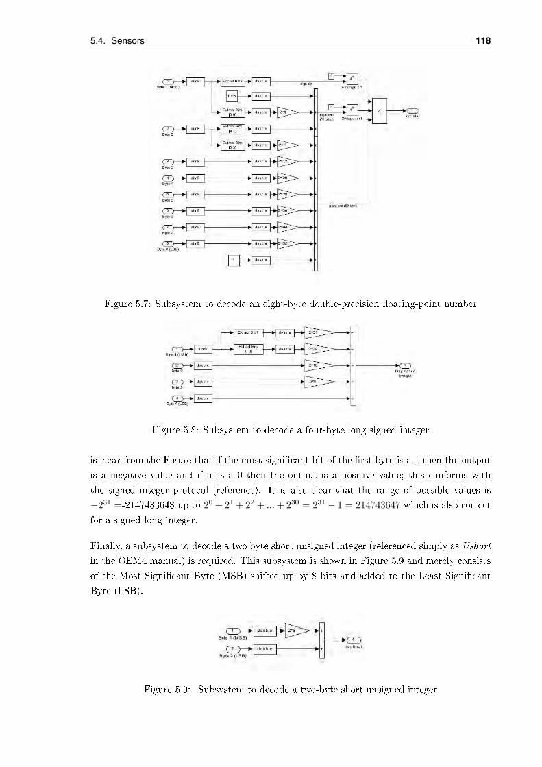
5.4. Sensors 118
Figure 5.7: Subsystem to decode an eight-byte double-precision oating-point number
Figure 5.8: Subsystem to decode a four-byte long signed integer
is clear from the Figure that if the most signicant bit of the rst byte is a 1 then the output
is a negative value and if it is a 0 then the output is a positive value; this conforms with
the signed integer protocol (reference). It is also clear that the range of possible values is
−231 =-2147483648 up to 20 + 21 + 22 + ...+ 230 = 231 − 1 = 214743647 which is also correct
for a signed long integer.
Finally, a subsystem to decode a two byte short unsigned integer (referenced simply as Ushort
in the OEM4 manual) is required. This subsystem is shown in Figure 5.9 and merely consists
of the Most Signicant Byte (MSB) shifted up by 8 bits and added to the Least Signicant
Byte (LSB).
Figure 5.9: Subsystem to decode a two-byte short unsigned integer

119 Chapter 5. State Estimation and Measurement
In future these four subsystems will be referred to as Float, Double, Long and Ushort respec-
tively, as per the OEM4 family manual [Novatel vol2 p12].
The Datum Transformations and Logic Subsystem The data passing out from the Data
Conversion subsystem then ows into the Datum Transformation and Logic subsystem. At
this stage the data contained in the individual elds, listed in Tables 5.1 and 5.2, are available
in a form directly compatible with Simulink. The Datum Conversion and Logic subsystem
performs the coordinate transformations to a datum which is directly compatible with the
Kalman Filter as well as performing logical operations to determine the validity of the position
and velocity solutions.
The process of transforming the coordinate system is now discussed. As has already been
mentioned, the BESTXYZ log outputs the position and velocity and their respective stan-
dard deviations in the ECEF coordinate system. However, the states dened in the state
matrix of the Kalman Filter, Equation (5.6), are referenced to the UTM coordinate system.
Clearly the necessary transformation then is from the ECEF coordinate system to the UTM
coordinate system. This conversion requires an intermediate conversion to the Geodetic co-
ordinate system and may therefore be described symbolically as
P (x, y, z)ECEF → P (λ, φ, h)GEO → P (E,N, h)UTM
where
P is the position
x, y and z are the ECEF coordinate axes as shown in Figure [ECEF picture in the lit review
(does not exist yet)]
λ is the longitude angle
φ is the latitude angle
h is the height above sea level
E is the Easting and
N is the Northing
Since the Earth is not a perfect sphere, the process of transforming the ECEF coordinate
system to the Geodetic coordinate system is not simple. The method of approximating the
Earth as an ellipsoid is widespread and so is selected for use. The ow of this process is shown
in Figure 5.10.
The inputs to the iteration are the vehicle position on the ECEF coordinate axes, (x, y, z),the semi-major axis of the Earth, a, and the semi-minor axis of the Earth, b. The earth model

5.4. Sensors 120
Figure 5.10: ECEF to Geodetic datum conversion iteration
which best approximates the region of interest (Adelaide, South Australia) is the Australian
Geodetic Datum (AGD84) which denes the ellipsoidal axes as
a = 6378160.0m
b = 6356774.719195289m
The algorithm of Figure 5.10 is written in an embedded MATLAB le within the Datum
Transformations and Logic subsystem shown in Figure 5.5. The arctan2 (y, x) function in
Figure 5.10 is a MATLAB-specic function similar to the conventional arctan yx . Note however
that if y < 0 and x < 0 then arctan2 (y, x) ∈ (−90,−180)o whereas arctan yx ∈ (0, 90)o - i.e.the arctan2 function outputs the angle in the correct quadrant, whereas the arctan function
does not.
The solution convergence of the algorithm is dened by the hk+1 ≈ hk and φk+1 ≈ φk criteriawithin the diamond shaped query block in Figure 5.10. These conditions basically state that
the iteration is complete once the solution does not change from one iteration step to the
next. This process is implemented in MATLAB code by determining the errors in height and
latitude from one iteration step to the next, i.e. eh = hk+1 − hk and eφ = φk+1 − φk. Oncethese errors fall below the user dened bounds, i.e. once eh < herror bound and eφ < φerror bound,
the solution has been solved. Data collected from the BESTXYZB log of the OEM4 GPS
unit indicated that an average of 8 iterations where necessary for the solution to converge

121 Chapter 5. State Estimation and Measurement
Figure 5.11: The datum transformation of the position standard deviation
below the bounds herror bound = 10−20m and φerror bound = 10−20rad, i.e. to virtually no
error. Implementation of the remainder of the algorithm is intuitive and therefore will not be
explained.
The next step is to transform the ECEF position standard deviations, (σx, σy, σz), velocities,(x, y, z, ), and velocity standard deviations, (σx, σy, σz), to the Geodetic datum. Unfortu-
nately, these data sets cannot simply be passed through the transformation algorithm in
Figure 5.10, since they are referenced to the current position, (x, y, z) , and not to the center
of the earth. One solution to this problem is to simply add the data set in question to the
current position in the ECEF datum, convert the new data set to the Geodetic datum using
the transformation algorithm and then subtract the Geodetic current position. This process
is described symbolically as
T (x2, y2, z2) = T (x1 + x2, y1 + y2, z + z2)− T (x1, y1, z1)
where (x1, y1, z1) is the ECEF position
(x2, y2, z2) is the ECEF position standard deviation, velocity, or velocity standard deviation
and the T () notation refers to datum transformation
To gain a better understanding, consider the case where the position standard deviation in
this case denoted, σP , is to be transformed from the ECEF datum to the Geodetic datum.
As shown in Figure 5.11 the position standard deviation is added vectorially to the position,
P1, still in the original ECEF coordinate frame, resulting in a new position vector, P2.
Both the new position, P2, and the original position, P1, are then transformed to the Geodetic
datum. Note that the position standard deviation, σP , is not transformed. The magnitude

5.4. Sensors 122
Figure 5.12: Vector visualisation of the longitudinal position standard deviation
of the position standard deviation in each of the three Geodetic dimensions is determined as
∆φσ = φ2 − φ1, ∆λσ = λ2 − λ1 and ∆hσ = h2 − h1, as depicted in Figures 5.12, 5.13 and
5.14.
The velocity and velocity standard deviations are computed identically to the position stan-
dard deviation. Note that this method involves treating the velocity and velocity standard
deviation as distance variables during the transformations and then re-interpreting these dis-
tances as velocities following the transformation.
Now that the procedure for converting the required variables from the ECEF datum to the
Geodetic datum has been fully described, the procedure for converting the variables from the
Geodetic datum to the Universal Transverse Mercator (UTM) is described. The Equations
which convert data in the Geodetic datum into data in the UTM datum are well documented.
However, it was found that when a set of Geodetic position-data was transformed with these
Equations into UTM data, the resulting plot was inexplicably rotated. Therefore a more sim-
plistic and intuitive approach, in which the earth is approximated as a sphere, was conceived.
Consider the Northing. Figure 5.15 shows a side view of the earth. The Northing, which is
the circumferential distance in the North direction is marked as N.
The Northing, N , relies on the radius of the Earth, R, and the change in Latitude, ∆φ.Mathematically it is calculated as the distance around the circumference of a sphere of radius
R, i.e.
N = R∆φ (5.26)
Due to the approximation of the Earth as a sphere, the smaller the change in Latitude which is
used, the more accurate the Northing value. The accuracy may also be improved by constantly

123 Chapter 5. State Estimation and Measurement
Figure 5.13: Vector visualisation of the latitudinal position standard deviation
Figure 5.14: Vector visualisation of the height position standard deviation

5.4. Sensors 124
Figure 5.15: The Northing
Figure 5.16: The Easting viewed looking down on the North Pole
updating the value of the radius which is dened as
R =√x2 + y2 + z2 (5.27)
where x, y and z are available from the ECEF coordinate system.
The derivation of the Easting is very similar to that of the Northing. Figure 5.16 shows a
Earth viewed looking down on the North Pole.
The Easting, E, relies on the change in longitude, ∆λ, and the projection of the radius of the
Earth at the current location onto the equatorial plane, Req, i.e.
E = Req∆λ

125 Chapter 5. State Estimation and Measurement
Figure 5.17: The Easting viewed looking at the Earth from the side
The projection of the radius of the Earth onto the equatorial plane is best determined from
the side view of the Earth, shown in Figure 5.17.
From Figure 5.17 it is clear that the projection of the radius of the Earth onto the equatorial
plane is dened as
Req = R cosφ
Therefore the Easting is dened as
E = R cosφ∆λ (5.28)
Due to the approximation of the Earth as a sphere, the smaller the change in Longitude which
is used, the more accurate the Easting value.
The height in the Geodetic datum requires no transformation into the UTM datum as the
denition of height in both datums is synonymous.
Equations (5.26) and (5.28), therefore fully dene the conversion from the Geodetic datum to
the UTM datum. To convert the Geodetic position to the UTM datum using these Equations,
an origin point, (λo, φo, ho), is determined. For the TARGET this point is selected as the
beginning of the vehicle path. The change in Latitude, ∆φ, required for Equation 5.15, is
calculated as the dierence between the current Latitude and origin Latitude, ie ∆φ = φ−φo.Similarly the change in Longitude, ∆λ, required for Equation (5.28), is calculated as the
dierence between the current Longitude and the origin longitude ∆λ = λ− λo.
The transformations of the position standard deviation, velocity and velocity standard devi-
ations are much more simple. Since these quantities have no specied location on the face of
the Earth and since the terms already refer to incremental changes in the Geodetic datum
axes, the change in Latitude term in Equation (5.26) is simply replaced by the Latitudinal
position standard deviation, Latitudinal velocity or Latitudinal velocity standard deviation.

5.4. Sensors 126
Similarly the change in Longitude term in Equation (5.28) is simply replaced by the Longi-
tudinal position standard deviation, Longitudinal velocity or Longitudinal velocity standard
deviation.
This completes the transformation from the ECEF datum to the UTM datum for the four
required variables. The stages of this conversion may be summarised as
1 Convert the ECEF position into the Geodetic datum, i.e.
(x, y, z)→ (λP , φP , hP )
2 Form ECEF pseudo position vectors for the position standard deviation, veloc-
ity and velocity standard deviations by adding them to the ECEF position and
transform these into the Geodetic datum, i.e.
(x+ σx, y + σy, z + σz)→ (λP+σP , φP+σP , hP+σP )
(x+ x, y + y, z + z)→ (λP+V , φP+V , hP+V )
(x+ σx, y + σx, z + σz)→ (λP+σV , φP+σV , hP+σV )
3 Subtract the Geodetic position from the Geodetic position standard-deviation, ve-
locity and velocity standard-deviation vectors to form the true position standard-
deviation, velocity and velocity standard deviation in the Geodetic datum, i.e.
(λσP = λP+σP − λP , φσP = φP+σp − φP , hσP = hP+σP − hP
)(λV = λP+V − λP , φV = φP+V − φP , hV = hP+V − hV )
(λσV = λP+σV − λP , φσV = φP+σV − φP , hσV = hP+σV − hP )
4 Transform the Geodetic position, position standard-deviation, velocity and veloc-
ity standard-deviations into the UTM datum using Equations (5.26) and (5.28),
i.e.
(λP , φP , hP )→ (EP , NP , hP )
(λσP , φσP , hσP )→ (EσP , NσP , hσP )

127 Chapter 5. State Estimation and Measurement
(λV , φV , hV )→ (EV , NV , hV )
(λσV , φσV , hσV )→ (EσV , NσV , hσV )
As implied by the name, the Datum Transformations and Logic subsystem contains code for
performing datum transformations and logical switching. The process of datum transforma-
tions, described in detail above, is reasonably complex and so is implemented with Embedded
MATLAB code for increased eciency. This code utilises the x, y, z, σx, σy, σz, x, y, z, σx,
σy and σz elds from Table 5.2. The remainder of the highlighted elds in Tables 5.1 and 5.2
are required for the switching logic. A brief overview of each of these elds and their use in
the Datum Transformations and Logic subsystem follows.
Idle Time The Idle Time eld indicates the percentage of the GPS card's Central Processing
Unit (CPU) in use. The Datum Transformations and Logic subsystem has the
option to log this quantity onto the TARGET computer so that, in the unlikely
event of GPS failure, the log le may be consulted to determine if the failure was
due to an overload of the GPS CPU.
Time Status The Time Status eld indicates the accuracy of the receiver's clock in relation to
the time decoded from the satellite ephemeris data. To provide an accurate posi-
tion solution, the satellite time must match the receiver clock, which is constantly
being steered to follow the satellite time. If the time error is too great then the
Time Status is set to the binary value equivalent to 20d or 130d. 20d occurs whenno ephemeris data has been decoded (generally only at startup) and 130d occurswhen the time error grows beyond a certain bound. The Datum Transformations
and Logic subsystem constantly compares the Time Status to these two values.
If either value is detected then the datum transformations (of all position and
velocity related quantities) are halted, and the current data set is not calculated.
However, Simulink requires subsystems to produce output quantities, therefore
the position and velocity quantities are arbitrarily set to 0 and output.
Milliseconds The Milliseconds eld provides the current number of milliseconds since the
beginning of the GPS week. The Datum Transformations and Logic subsystem
uses this value to ensure that one set of GPS position data is only ever trans-
formed once. This ensures that TARGET CPU does not overload by attempting
to execute the datum transformations more frequently than necessary.
Receiver Status The Receiver Status eld contains information on 32 dierent hardware and
software errors which the GPS unit may suer. Only two of these errors are deemed
critical - the temperature error and the voltage supply error. The temperature
error indicates that the OEM4 card has either overheated or underheated, and
the voltage supply error indicates that the voltage to the OEM4 card is either
too high or too low. If the Datum Transformations and Logic subsystem detects

5.4. Sensors 128
either of these critical errors, the failure-mode ag is set and the TARGET vehicle
comes to a halt. The GPS unit may then be inspected for damage, hopefully
before the damage becomes too severe. Other Receiver Status indicators which
provide information on errors which are non-critical are the (GPS card) CPU
overload ag, the (GPS card) COM1 buer overrun ag, the almanac ag and the
position solution ag. If any of these errors occurs the datum transformations on
the data are temporarily prevented and the position and velocity error ags are
set. The CPU overload ag is set when the GPS card CPU attempts to process
to much data at too high a rate; the eect of a CPU overload is random loss
of data. Consequently, the position or velocity related terms output from the
unit may be incorrect if the CPU overloads. If this is the case then it is a waste
of the TARGET CPU to perform the datum conversions; hence the conversions
are prevented and the position and velocity error ags are set. The eect of an
OEM4 COM1 buer overrun (this is the serial port on the OEM4 card which
is connected to the TARGET computer) is identical to when the CPU overloads,
hence the logic deals with these two errors in the same manner. The almanac error
and the position solution error both essentially mean that the position solution
cannot be calculated by the OEM4 unit. It is therefore appropriate to cancel the
datum conversions and set the position error ag. As discussed in the Literature
Review, the GPS unit calculates velocity using doppler measurements which rely
on the position; if the position is not available then the velocity cannot be correct
and so for the alamanac error and the position solution error the velocity error ag
within the Datum Transformations and Logic subsystem is also set. The entire
Receiver Status eld is also logged to the TARGET computer so that the hardware
and software errors which occurred with the OEM4 unit during the run may be
inspected.
Position Solution Status The Position Solution Status eld indicates the level of accuracy of
the position solution as calculated by the OEM4. The Position Solution Status is
set to 0 to indicates that the position solution is acceptable. Other values in this
eld correspond to position solutions which may not give position errors in the
Receiver Status eld but which may be unpredictable in terms of their accuracy.
Therefore if the value of the position solution status eld is not zero then the
position error ag within the Datum Transformations and Logic subsystem is set
and the datum transformation process is temporarily halted.
Velocity Solution Status The Velocity Solution Status eld is equivalent the position solution
status eld, except that it relates only to the velocity. If this eld returns any value
other than 0 it indicates that the velocity is not valid. Note that it is possible for
the position to be valid and the velocity invalid (for example if only one position
measurement is taken then the doppler velocity cannot be known), therefore if
this eld is a non-zero value then only the velocity error ag within the Datum
Transformations and Logic subsystem is set and only the velocity-related terms
are prevented from entering the datum transformation process.

129 Chapter 5. State Estimation and Measurement
Number of GPS L1 Ranges in Use This eld states the number of GPS satellites which are
currently visible and who's ephemeris data is being used to compute the position
solution. The eld is logged to the TARGET computer for interest's sake.
Velocity Latency This eld provides the exact number of seconds since the velocity solution
was calculated (to single precision oating point accuracy). This value is used to
determine if the velocity solution is current or not. If it is not current then the
datum of the velocity related terms is not transformed since this would simply
involve re-transforming the same data. Also, if the velocity is current, the Datum
Transformations and Logic subsystem velocity error ag is set.
Note that all position error ags mentioned above are AND'ed together, as are the veloc-
ity error ags. These error ags always occur in conjunction with the appropriate datum
transformation being canceled (i.e. the position related variables are canceled in the case of
a position error ag and the velocity-related variables are canceled in the case of a velocity
error ag). These ag are then passed to the Kalman Filter, along with the UTM-referenced
position and velocity data.
5.4.1.3 Integrating the GPS Sensor into the Kalman Filter
Section 5.4.1.2 describes the inner workings of the GPS data decoding program. The pur-
pose of this program is to transform the geometric GPS data into a form which may be
eciently integrated into the Kalman Filter. The geometric data which ows out of the de-
coding program and into the Kalman Filter consists of the position, the velocity, the position
standard deviation and the velocity standard deviation, all referenced to the UTM datum,
i.e.[(E,N, h) ,
(E, N , h
), (σE , σN , σh) ,
(σE , σN , σh
)]. Since it is possible that the position
data will be available when the velocity data is not, the state update Equations are divided
into two sets of Equations - GPS position updates and GPS velocity updates. Each of these
sets of Equations contains a measurement vector, a measurement matrix and a sensor noise
covariance matrix. These matrices and vectors are required to form the Kalman gain matrix
which in turn will update the states vector and state covariance matrix.
Velocity State Updates from the GPS Unit The measurement vector for the GPS velocity,
yGPS−V , is dened as Equation (5.29).
yGPS−V =
[E
N
](5.29)
Note that the vertical speed, h, is omitted from this vector since the vehicle is assumed to
travel only on at ground. The rst step in deriving the measurement matrix for the velocity
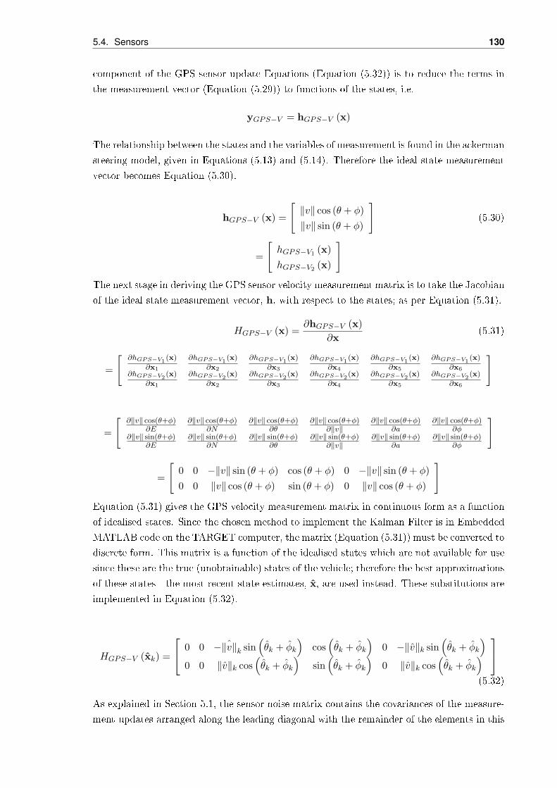
5.4. Sensors 130
component of the GPS sensor update Equations (Equation (5.32)) is to reduce the terms in
the measurement vector (Equation (5.29)) to functions of the states, i.e.
yGPS−V = hGPS−V (x)
The relationship between the states and the variables of measurement is found in the ackerman
steering model, given in Equations (5.13) and (5.14). Therefore the ideal state measurement
vector becomes Equation (5.30).
hGPS−V (x) =
[‖v‖ cos (θ + φ)‖v‖ sin (θ + φ)
](5.30)
=
[hGPS−V1 (x)hGPS−V2 (x)
]The next stage in deriving the GPS sensor velocity measurement matrix is to take the Jacobian
of the ideal state measurement vector, h, with respect to the states; as per Equation (5.31).
HGPS−V (x) =∂hGPS−V (x)
∂x(5.31)
=
[∂hGPS−V1
(x)
∂x1
∂hGPS−V1(x)
∂x2
∂hGPS−V1(x)
∂x3
∂hGPS−V1(x)
∂x4
∂hGPS−V1(x)
∂x5
∂hGPS−V1(x)
∂x6∂hGPS−V2
(x)
∂x1
∂hGPS−V2(x)
∂x2
∂hGPS−V2(x)
∂x3
∂hGPS−V2(x)
∂x4
∂hGPS−V2(x)
∂x5
∂hGPS−V2(x)
∂x6
]
=
[∂‖v‖ cos(θ+φ)
∂E∂‖v‖ cos(θ+φ)
∂N∂‖v‖ cos(θ+φ)
∂θ∂‖v‖ cos(θ+φ)
∂‖v‖∂‖v‖ cos(θ+φ)
∂a∂‖v‖ cos(θ+φ)
∂φ∂‖v‖ sin(θ+φ)
∂E∂‖v‖ sin(θ+φ)
∂N∂‖v‖ sin(θ+φ)
∂θ∂‖v‖ sin(θ+φ)
∂‖v‖∂‖v‖ sin(θ+φ)
∂a∂‖v‖ sin(θ+φ)
∂φ
]
=
[0 0 −‖v‖ sin (θ + φ) cos (θ + φ) 0 −‖v‖ sin (θ + φ)0 0 ‖v‖ cos (θ + φ) sin (θ + φ) 0 ‖v‖ cos (θ + φ)
]Equation (5.31) gives the GPS velocity measurement matrix in continuous form as a function
of idealised states. Since the chosen method to implement the Kalman Filter is in Embedded
MATLAB code on the TARGET computer, the matrix (Equation (5.31)) must be converted to
discrete form. This matrix is a function of the idealised states which are not available for use
since these are the true (unobtainable) states of the vehicle; therefore the best approximations
of these states - the most recent state estimates, x, are used instead. These substitutions are
implemented in Equation (5.32).
HGPS−V (xk) =
0 0 − ˆ‖v‖k sin(θk + φk
)cos(θk + φk
)0 −‖v‖k sin
(θk + φk
)0 0 ‖v‖k cos
(θk + φk
)sin(θk + φk
)0 ‖v‖k cos
(θk + φk
) (5.32)
As explained in Section 5.1, the sensor noise matrix contains the covariances of the measure-
ment updates arranged along the leading diagonal with the remainder of the elements in this

131 Chapter 5. State Estimation and Measurement
square matrix set to zero. The measurement noise matrix for the velocity component of the
GPS sensor update is given as Equation (5.33).
RGPS−Vk =
σ2EGPSk
0
0 σ2NGPSk
(5.33)
The current Easting-rate covariance, σ2EGPSk
, and Northing-rate covariance, σ2NGPSk
, are sim-
ply the square of the standard deviations which are output from the Datum Transformations
and Logic subsystem to the Kalman Filter subsystem within the TARGET computer pro-
gram. As the GPS unit provides a measure of the accuracy of its own velocity solution, in the
form of velocity standard deviations, the GPS velocity sensor noise matrix may be constantly
updated. This ensures that the Kalman Filter correctly updates the states, such that the best
possible state estimates are returned.
Note that the Kalman Filter is designed under the assumption that the sensor measurements
of the elements of the velocity measurement vector (5.29) are randomly distributed with zero-
mean. Essentially this means that both the Easting velocity and the Northing velocity as
output from the GPS sensor may have noise, providing that it is distributed such that the
mean lies on the true Easting and Northing velocities. Section 5.4.1.4 will show from test
data that this is approximately the case.
All of the matrices required to calculate the instantaneous Kalman gain matrix, given as
Equation (5.34), have now been determined. The 6× 6 matrix of state estimate covariances,
P−k , used to calculate this matrix, is available either from the vehicle model a-priori covariance
(see Equation (5.2)) or from the posteriori covariance of any of the sensors which may have
been used to correct the states of the vehicle model (Equations (5.36), (5.43) and [waiting for
hall eect sensor]).
KGPS−Vk = P−k HTGPS−Vk
(HGPS−VkP
−k H
TGPS−Vk +RGPS−Vk
)−1(5.34)
The error between the current GPS velocity sensor states , yGPS−Vk , and the current state
estimates transformed into the same dimensions as the GPS velocity sensor states, h (xk), isthen multiplied by the Kalman gain matrix and added to the previous estimate of the vehicle
states. This process, given as Equation (5.35), optimally updates the states based on the
most recent velocity data from the GPS unit.
xk = x−k +KGPS−Vk (yGPS−V − h (xk)) (5.35)
The state covariance matrix, P , dened as Equation (5.36), is also updated to give a measure
of the accuracy of the state update which just occurred.
Pk = (I −KGPS−VkHGPS−Vk)P−k (5.36)
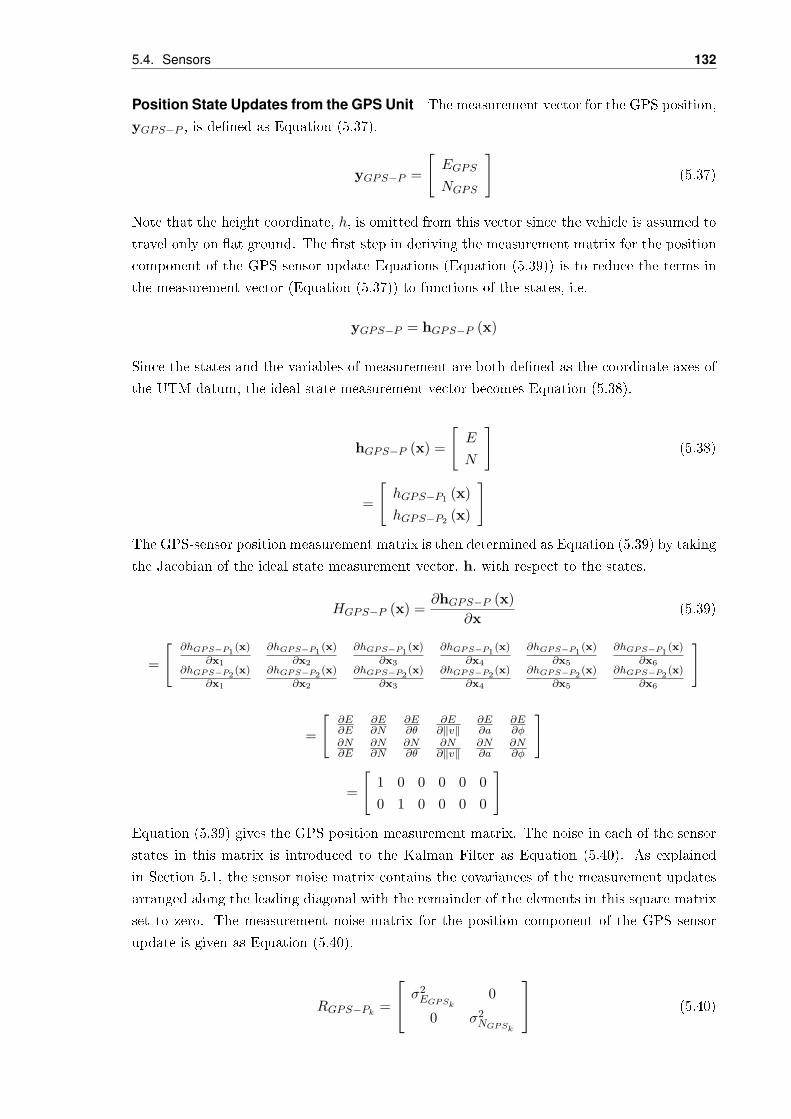
5.4. Sensors 132
Position State Updates from the GPS Unit The measurement vector for the GPS position,
yGPS−P , is dened as Equation (5.37).
yGPS−P =
[EGPS
NGPS
](5.37)
Note that the height coordinate, h, is omitted from this vector since the vehicle is assumed to
travel only on at ground. The rst step in deriving the measurement matrix for the position
component of the GPS sensor update Equations (Equation (5.39)) is to reduce the terms in
the measurement vector (Equation (5.37)) to functions of the states, i.e.
yGPS−P = hGPS−P (x)
Since the states and the variables of measurement are both dened as the coordinate axes of
the UTM datum, the ideal state measurement vector becomes Equation (5.38).
hGPS−P (x) =
[E
N
](5.38)
=
[hGPS−P1 (x)hGPS−P2 (x)
]The GPS-sensor position measurement matrix is then determined as Equation (5.39) by taking
the Jacobian of the ideal state measurement vector, h, with respect to the states.
HGPS−P (x) =∂hGPS−P (x)
∂x(5.39)
=
[∂hGPS−P1
(x)
∂x1
∂hGPS−P1(x)
∂x2
∂hGPS−P1(x)
∂x3
∂hGPS−P1(x)
∂x4
∂hGPS−P1(x)
∂x5
∂hGPS−P1(x)
∂x6∂hGPS−P2
(x)
∂x1
∂hGPS−P2(x)
∂x2
∂hGPS−P2(x)
∂x3
∂hGPS−P2(x)
∂x4
∂hGPS−P2(x)
∂x5
∂hGPS−P2(x)
∂x6
]
=
[∂E∂E
∂E∂N
∂E∂θ
∂E∂‖v‖
∂E∂a
∂E∂φ
∂N∂E
∂N∂N
∂N∂θ
∂N∂‖v‖
∂N∂a
∂N∂φ
]
=
[1 0 0 0 0 00 1 0 0 0 0
]Equation (5.39) gives the GPS position measurement matrix. The noise in each of the sensor
states in this matrix is introduced to the Kalman Filter as Equation (5.40). As explained
in Section 5.1, the sensor noise matrix contains the covariances of the measurement updates
arranged along the leading diagonal with the remainder of the elements in this square matrix
set to zero. The measurement noise matrix for the position component of the GPS sensor
update is given as Equation (5.40).
RGPS−Pk =
σ2EGPSk
0
0 σ2NGPSk
(5.40)
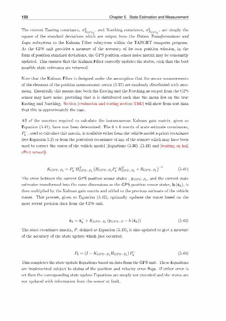
133 Chapter 5. State Estimation and Measurement
The current Easting covariance, σ2EGPSk
, and Northing covariance, σ2NGPSk
, are simply the
square of the standard deviations which are output from the Datum Transformations and
Logic subsystem to the Kalman Filter subsystem within the TARGET computer program.
As the GPS unit provides a measure of the accuracy of its own position solution, in the
form of position standard deviations, the GPS position sensor noise matrix may be constantly
updated. This ensures that the Kalman Filter correctly updates the states, such that the best
possible state estimates are returned.
Note that the Kalman Filter is designed under the assumption that the sensor measurements
of the elements of the position measurement vector (5.37) are randomly distributed with zero-
mean. Essentially this means that both the Easting and the Northing as output from the GPS
sensor may have noise, providing that it is distributed such that the mean lies on the true
Easting and Northing. Section [evaluation and testing section TBD] will show from test data
that this is approximately the case.
All of the matrices required to calculate the instantaneous Kalman gain matrix, given as
Equation (5.41), have now been determined. The 6× 6 matrix of state estimate covariances,
P−k , used to calculate this matrix, is available either from the vehicle model a-priori covariance
(see Equation 5.2) or from the posteriori covariance of any of the sensors which may have been
used to correct the states of the vehicle model (Equations (5.36) ,(5.43) and [waiting on hall
eect sensor]).
KGPS−Pk = P−k HTGPS−Pk
(HGPS−PkP
−k H
TGPS−Pk +RGPS−Pk
)−1(5.41)
The error between the current GPS position sensor states , yGPS−Pk , and the current state
estimates transformed into the same dimensions as the GPS position sensor states, h (xk), isthen multiplied by the Kalman gain matrix and added to the previous estimate of the vehicle
states. This process, given as Equation (5.42), optimally updates the states based on the
most recent position data from the GPS unit.
xk = x−k +KGPS−Pk (yGPS−P − h (xk)) (5.42)
The state covariance matrix, P , dened as Equation (5.43), is also updated to give a measure
of the accuracy of the state update which just occurred.
Pk = (I −KGPS−PkHGPS−Pk)P−k (5.43)
This completes the state update Equations based on data from the GPS unit. These Equations
are implemented subject to status of the position and velocity error ags. If either error is
set then the corresponding state update Equations are simply not executed and the states are
not updated with information from the sensor at fault.
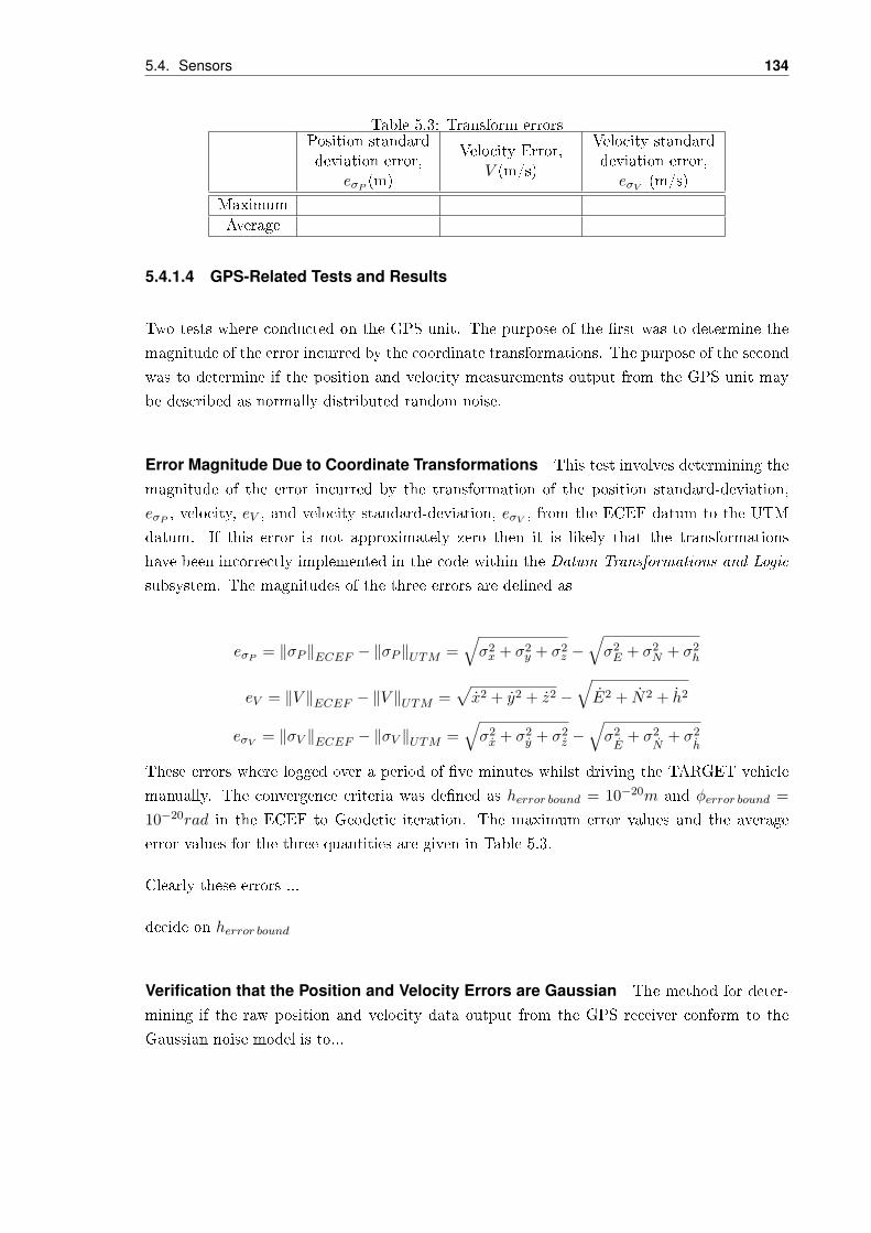
5.4. Sensors 134
Table 5.3: Transform errorsPosition standarddeviation error,
eσP (m)
Velocity Error,V (m/s)
Velocity standarddeviation error,eσV (m/s)
Maximum
Average
5.4.1.4 GPS-Related Tests and Results
Two tests where conducted on the GPS unit. The purpose of the rst was to determine the
magnitude of the error incurred by the coordinate transformations. The purpose of the second
was to determine if the position and velocity measurements output from the GPS unit may
be described as normally distributed random noise.
Error Magnitude Due to Coordinate Transformations This test involves determining the
magnitude of the error incurred by the transformation of the position standard-deviation,
eσP , velocity, eV , and velocity standard-deviation, eσV , from the ECEF datum to the UTM
datum. If this error is not approximately zero then it is likely that the transformations
have been incorrectly implemented in the code within the Datum Transformations and Logic
subsystem. The magnitudes of the three errors are dened as
eσP = ‖σP ‖ECEF − ‖σP ‖UTM =√σ2x + σ2
y + σ2z −
√σ2E + σ2
N + σ2h
eV = ‖V ‖ECEF − ‖V ‖UTM =√x2 + y2 + z2 −
√E2 + N2 + h2
eσV = ‖σV ‖ECEF − ‖σV ‖UTM =√σ2x + σ2
y + σ2z −
√σ2E
+ σ2N
+ σ2h
These errors where logged over a period of ve minutes whilst driving the TARGET vehicle
manually. The convergence criteria was dened as herror bound = 10−20m and φerror bound =10−20rad in the ECEF to Geodetic iteration. The maximum error values and the average
error values for the three quantities are given in Table 5.3.
Clearly these errors ...
decide on herror bound
Verification that the Position and Velocity Errors are Gaussian The method for deter-
mining if the raw position and velocity data output from the GPS receiver conform to the
Gaussian noise model is to...
135 Chapter 5. State Estimation and Measurement
Figure 5.18: I need a caption...and a picture (TBD)
5.4.2 Inertial Measurement Unit Sensor
The chosen Inertial Measurement Unit (IMU) sensor is a Microstrain 3DM-GX1, Firmware
Version 3.1.02. The IMU processing card is housed within a sealed enclosure which protects it
from dust, water and other elements. This enclosure is xed to the oor pan of the TARGET
vehicle vertically above the rear dierential, as shown in Figure 5.18.
The 3DM-GX1 combines the data from three angular rate gyroscopes, three orthogonal ac-
celerometers and three orthogonal magnetometers to output the attitude, the attitude rate
and the acceleration in the three orthogonal axes. The IMU interfaces with the TARGET
computer via a serial RS232 connection.
5.4.2.1 Device Configuration
The speed of the serial port of the 3DM-GX1 was determined by plugging the unit into a
PC running Windows XP and running the Data Acquisition and Display software designed
specically for the 3DM-GX1. The serial port speed was found to be 115200 baud. For the
purposes of calibration, Section 5.4.4.2 requires the values which lie in registers 130 and 230
in the 3DM-GX1's EEPROM. These values where found to be 8500 and 13000 by again using
the Data Acquisition and Display software to read the EEPROM addresses. The 3DM-GX1
was then disconnected from the PC and connected to the TARGET computer, which was set
up to match the rate of the serial port.
Data is retrieved from the 3DM-GX1 by sending it one of the byte-sized commands listed
in the instruction set through the serial connection. Depending on the command, the re-
sponse may consist of the raw data from the accelerometers, gyros and magnetometers, the
temperature of the unit, the orthogonalised acceleration, the instantaneous Euler angles, the
gyro-stabilised Euler angles, the instantaneous angular rates and the compensated angular
rates. The command selected for use in the TARGET vehicle project was command 0x31.
In response to this command the 3DM-GX1 outputs the gyro-stabilised Euler angles, the
orthogonalised acceleration, the compensated angular rates, a time stamp and a checksum.
These values are output in the form of signed or unsigned short integers (i.e. two bytes each)
and must be scaled by the appropriate gains to transform the data into the correct units.
The checksum is useful for ensuring that the data transmitted from the 3DM-GX1 to the
TARGET computer is complete and the timstamp is used to determine if new data has been
received.
5.4.2.2 Data Decoding Program
The high-level structure of the IMU data decoding program and its interface to the Kalman
Filter is shown in the ow diagram of Figure 5.19.

5.4. Sensors 136
Figure 5.19: The IMU data decoding program
Table 5.4: Response of the 3DM-GX1 to the 0x31 commandField Name Field Data Type
Header Byte Short Uint
Roll MSB Short Uint
Roll LSB Short Uint
Pitch MSB Short Uint
Pitch LSB Short Uint
Yaw MSB Short Uint
Yaw LSB Short Uint
X acceleration MSB Short Int
X acceleration LSB Short Int
Y acceleration MSB Short Int
Y acceleration LSB Short Int
Z acceleration MSB Short Int
Z acceleration LSB Short Int
Roll rate MSB Short Int
Roll rate LSB Short Int
Pitch rate MSB Short Int
Pitch rate LSB Short Int
Yaw rate MSB Short Int
Yaw rate LSB Short Int
Timer ticks MSB Short Uint
Timer ticks LSB Short Uint
Checksum MSB Short Uint
Checksum LSB Short Uint
Figure 5.19 indicates that the IMU data emerges from the serial port as a vector of individual
bytes which is then decoded into decimal values by the IMU Data Conversion subsystem.
This subsystem both scales the data into the correct units for the Kalman Filter and performs
logical checks on the data to determined its validity.
To best explain the functioning of the IMU Data Conversion and Logic subsystem it is nec-
essary to discuss the incoming data from the serial port. As has been mentioned, this data
corresponds to the response of the 3DM-GX1 to the 0x31 command and is organised as a
set of 23 individual bytes. The specic bytes resulting from the 0x31 command are shown in
Table 5.4.
The rst entry of Table 5.4, the header byte, is used by the TARGET computer to determine

137 Chapter 5. State Estimation and Measurement
Figure 5.20: Subsystem to decode a short signed integer
the beginning of the response. Since this byte always has the same value as the command
value (31H = 49d) the TARGET computer simply waits for this value before reading the
entire response into the program. Once the response enters the program, only the elds which
are highlighted are used and the remainder of the elds are terminated. The elds of data
type short Uint are combined into a form more intelligible to Simulink by simply multiplying
the most signicant byte (MSB) by 28 (i.e.shifting it up by 8 bits) and adding it to the
least signicant byte (LSB). This subsystem has already been implemented in the GPS data
decoding program and is given as Figure [Figure: short uint]. The conversion from two bytes
to a single signed value is similar, except that the most signicant bit of the most signicant
byte is used to determine the sign of the nal value. The subsystem used to implement this
procedure is shown in Figure 5.20.
Once all of the individual bytes have been decoded, the normalisation and transformation
process is executed. This process involves multiplying the decoded values by a given constant
to transform them into the desired units, and ensuring that the denitions of the values
matches that expected by the Kalman Filter. Note that only the highlighted values in Table
5.4 are required and hence are normalised and transformed.
The yaw is transformed into degrees by multiplying the decoded value by 36065535 . The value of
the yaw is then biased to ensure that zero is output when the unit is racing due East. This
is the denition of the yaw (which up until this point has been called the heading) as given
in Figure 5.2. The yaw is also subtracted from the value 360 to ensure that rotations in the
anticlockwise direction yield positive values. The yaw enters the Kalman Filter in degrees
where it is promptly converted to radians.
The accelerations are transformed into the units of meters per second per second by multi-
plying the decoded values by 9.81Reg23032768000 , where Reg230 = 13000 was determined in Section
5.4.4.1. No modications to the accelerations are required before passing them to the Kalman
Filter.
The yaw rate is transformed into the units of degrees per second by multiplying the decoded
values by Reg13032768000 , where Reg130 = 8500 was determined in Section 5.4.4.1. This value
5.4. Sensors 138
requires multiplication by −1 to ensure that anticlockwise rotations yield positive yaw rate
values, the convention used in the Kalman Filter.
Scaling is not performed on the Checksum eld, since this eld is used to determine if the
incoming data is valid. The checksum must be equal to the sum of all the previous bytes
(determined as the LSBs added together and then added the sum of the MSBs shifted up by
8 bits). If this checksum fails then an error ag is set within the IMU data decoding program.
This error ag may also be set if any of the yaw, x acceleration, y acceleration and yaw rate
are out of their predened ranges or move at an unacceptable rate from one time step to the
next. The values of these ranges and rates are determined with the tests described in Section
5.4.3.4.
As will be discussed in Section 5.4.4.3, the timer-ticks are merely required by the Kalman
Filter to determine if the incoming data is new, therefore the timer ticks are left unscaled,
rather than scaling them to the same units as time.
5.4.2.3 Integrating the IMU Data into the Kalman Filter
Under the assumption that the TARGET vehicle drives only on at ground, the pitch, roll,
z-acceleration, pitch rate and roll rate are always zero and so are of no assistance in relation
to the vehicle states. The measurement vector for the IMU, \mathbfy_IMU, is therefore
dened to include the states which do vary as the vehicle drives on at ground, namely those
given in Equation (5.44).
yIMU =
xIMU
yIMU
θIMU
θIMU
(5.44)
where x is the x-acceleration or forward acceleration, y is the y-acceleration normal accelera-
tion, θ is the yaw or heading and θ is the yaw rate or heading rate. The rst step in deriving
the measurement matrix for the IMU sensor update Equations (Equation (5.51)) is to reduce
the terms in the measurement vector (Equation (5.44)) to functions of the states, i.e.
yIMU = hIMU (x)
The IMU forward acceleration, xIMU , and the heading, θIMU , terms are directly equivalent
to the states a and θ . However the normal acceleration, yIMU , and the heading rate, θIMU ,
are not so easily obtained. The heading rate may be written as a function of the states using
a property of the Ackerman steering model given by Equation (5.45), [reference].
θ =‖v‖L
tanφ (5.45)

139 Chapter 5. State Estimation and Measurement
For the tangential acceleration, the Equation of motion for a body under rotation, Equation
(5.46) is used.
y =‖v‖2
R(5.46)
where R is the radius of the instantaneous circular path. This radius may be determined from
the Ackerman steering model as Equation (5.47).
R =‖v‖θ
(5.47)
Substituting Equation (5.45) into Equation (5.47), yields Equation (5.48).
R =L
tanφ(5.48)
Then substituting Equation (5.48) into Equation (5.46) gives Equation(5.49).
y =‖v‖2 tanφ
L(5.49)
An ideal IMU sensor would therefore be expressible as a function of the states, as given by
Equation (5.50).
xIMU
yIMU
θIMU
θIMU
=
a
‖v‖2 tanφL
θ‖v‖ tanφ
L
(5.50)
=
hIMU1 (x)hIMU2 (x)hIMU3 (x)hIMU4 (x)
The IMU sensor measurement matrix is then determined as Equation (5.51) by taking the
Jacobian of the ideal state measurement vector, h, with respect to the states.
HIMU (x) =∂hIMU (x)
∂x(5.51)
=
∂hIMU1
(x)
∂x1
∂hIMU1(x)
∂x2
∂hIMU1(x)
∂x3
∂hIMU1(x)
∂x4
∂hIMU1(x)
∂x5
∂hIMU1(x)
∂x6∂hIMU2
(x)
∂x1
∂hIMU2(x)
∂x2
∂hIMU2(x)
∂x3
∂hIMU2(x)
∂x4
∂hIMU2(x)
∂x5
∂hIMU2(x)
∂x6∂hIMU3
(x)
∂x1
∂hIMU3(x)
∂x2
∂hIMU3(x)
∂x3
∂hIMU3(x)
∂x4
∂hIMU3(x)
∂x5
∂hIMU3(x)
∂x6∂hIMU4
(x)
∂x1
∂hIMU4(x)
∂x2
∂hIMU4(x)
∂x3
∂hIMU4(x)
∂x4
∂hIMU4(x)
∂x5
∂hIMU4(x)
∂x6
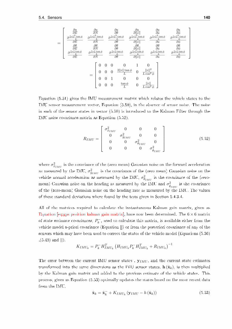
5.4. Sensors 140
=
∂a∂E
∂a∂N
∂a∂θ
∂a∂‖v‖
∂a∂a
∂a∂φ
∂‖v‖2 tanφ
L∂E
∂‖v‖2 tanφ
L∂N
∂‖v‖2 tanφ
L∂θ
∂‖v‖2 tanφ
L∂‖v‖
∂‖v‖2 tanφ
L∂a
∂‖v‖2 tanφ
L∂φ
∂θ∂E
∂θ∂N
∂θ∂θ
∂θ∂‖v‖
∂θ∂a
∂θ∂φ
∂‖v‖ tanφ
L∂E
∂‖v‖ tanφ
L∂N
∂‖v‖ tanφ
L∂θ
∂‖v‖ tanφ
L∂‖v‖
∂‖v‖ tanφ
L∂a
∂‖v‖ tanφ
L∂φ
=
0 0 0 0 1 0
0 0 0 2‖v‖ tanφL 0 ‖v‖2
L cos2 φ
0 0 1 0 0 00 0 0 tanφ
L 0 ‖v‖L cos2 φ
Equation (5.51) gives the IMU measurement matrix which relates the vehicle states to the
IMU sensor measurement vector, Equation (5.50), in the absence of sensor noise. The noise
in each of the sensor states in vector (5.50) is introduced to the Kalman Filter through the
IMU noise covariance matrix as Equation (5.52).
RIMU =
σ2xIMU
0 0 00 σ2
yIMU0 0
0 0 σ2θIMU
00 0 0 σ2
θIMU
(5.52)
where σ2xIMU
is the covariance of the (zero-mean) Gaussian noise on the forward acceleration
as measured by the IMU, σ2yIMU
is the covariance of the (zero-mean) Gaussian noise on the
vehicle normal acceleration as measured by the IMU, σ2θIMU
is the covariance of the (zero-
mean) Gaussian noise on the heading as measured by the IMU and σ2θIMU
is the covariance
of the (zero-mean) Gaussian noise on the heading rate as measured by the IMU. The values
of these standard deviations where found by the tests given in Section 5.4.3.4.
All of the matrices required to calculate the instantaneous Kalman gain matrix, given as
Equation [eq:gps position kalman gain matrix], have now been determined. The 6× 6 matrix
of state estimate covariances, P−k , used to calculate this matrix, is available either from the
vehicle model a-priori covariance (Equation []) or from the posteriori covariance of any of the
sensors which may have been used to correct the states of the vehicle model (Equations (5.36)
,(5.43) and []).
KIMUk = P−k HTIMUk
(HIMUkP
−k H
TIMUk
+RIMUk
)−1
The error between the current IMU sensor states , yIMU , and the current state estimates
transformed into the same dimensions as the IMU sensor states, h (xk), is then multiplied
by the Kalman gain matrix and added to the previous estimate of the vehicle states. This
process, given as Equation (5.53) optimally updates the states based on the most recent data
from the IMU.
xk = x−k +KIMUk (yIMU − h (xk)) (5.53)

141 Chapter 5. State Estimation and Measurement
Figure 5.21: Mounted hall eect sensor (TBD)
The state covariance matrix, P, dened as Equation (5.54), is also updated to give a measure
of the accuracy of the state update which just occurred.
Pk = (I −KIMUkHIMUk)P−k (5.54)
This completes the state update Equations based on data from the IMU sensor. These
Equations are implemented if the error ag output by the IMU Data Conversion and Logic
subsystem is zero and if the timestamp output from this same subsystem has changed since
the previous IMU sensor update. If either of these is zero then the state update Equations are
simply not executed and the vehicle states are not updated with information from the IMU
sensor.
5.4.2.4 IMU-Related Tests and Results
determine σ2xIMU
, σ2yIMU
, σ2θIMU
, σ2θIMU
.
5.4.3 Hall-Effect Sensor
A Hall-eect sensor is a device which measures magnetic elds. For the purposes of vehicle
state estimation, Hall-eect sensors are generally placed over some component of the drive
train mechanism to measure the vehicle speed (or a multiple thereof). [motivation for use in
lter] The Hall-eect sensor therefore provides data which may be used to update the vehicle
speed in the Kalman Filter.
5.4.3.1 Device Configuration
The Hall-eect sensor installed in the Target vehicle is a Honeywell GT1 series 1GT101DC
solid state Hall-eect sensor. The sensor is mounted on the underside of the vehicle facing
the drive shaft. As shown in Figure 5.21, four evenly-spaced steel lobes are attached to the
drive shaft beneath the sensor. As the vehicle moves forward, the drive shaft turns and the
steel lobes pass under the sensor.
During the time period when the lobe is under the sensor the voltage of the signal line is
pulled up to 5 volts thorough a 1kΩ resistor. Once the lobe has moved from under the sensor
the voltage drops back to ground again, eectively resulting in a pulse wave. The high time
of the output pulse wave is equal to the duration of time that each lobe is beneath the sensor
and the period of the wave is equal to the time between two successive lobes passing under

5.4. Sensors 142
Figure 5.22: Hall eect sensor setup (TBD)
the sensor. The signal line is connected to the Measurement Computing PCI-CTR05 card of
the XPC Target computer, a diagram of this setup is shown in Figure 5.22.
The CTR05 card detects each rising edge of the incoming pulse wave. The card measures the
time period between these riding edges and converts this to the frequency which is available as
an output from the FM TEST Simulink block in the XPC library. For most accurate results
the FM TEST Simulink block must be congured with the expected incoming frequency
range. This range will vary from 0Hz when the drive shaft is not turning to a maximum fre-
quency corresponding to the maximum vehicle speed. This maximum frequency is determined
from Equation 5.55
f =nlobeskDiff‖v‖
2πR(5.55)
where
nlobes is the number of lobes axed to the shaft beneath the sensor (in the case of the TARGET
this is 4).
kDiff is the di-ratio specic to the vehicle (in the case of the TARGET this is 4.875 - ie for
every 4.875 rotations of the driveshaft the rear wheels rotate once)
‖v‖is the vehicle speed
R is the average radius of the wheels (0.32m is suciently accurate for this estimate)
If the maximum vehicle speed to be monitored by the Hall-eect sensor is 60km/hr ie
16.67m/s then f = 161.6Hz. The FM TEST block is therefore set up for a frequency
rage of f ∈ [0, 170]Hz.
5.4.3.2 Data Decoding Program
5.4.3.3 Integrating the IMU Data into the Kalman Filter
As always it is necessary to model the data from the sensing system so that any errors may
be predicted and corrected either by the Kalman Filter or by some other error checking
and correcting program. The faults existent in this subsystem under normal operation (ie
excluding failure modes) are listed from most severe to least severe:
1 The PCI-CTR05 card lower bound rounding
2 Variation in wheel radius
3 Refresh rates

143 Chapter 5. State Estimation and Measurement
4 The PCI-CTR05 card upper bound rounding
5 Driveshaft movement in relation to the Hall-eect sensor
6 The PCI-CTR05 card quantisation error
The rst fault results when a pulse wave of too low a frequency is input into the PCI-CTR05
card. With the conguration described in Section 4.2.2.2, the minimum frequency which may
be accurately measured is 0.2Hz. Frequencies below this limit will result in an output value
of 50000Hz. If this frequency is allowed to enter the Kalman Filter then the speed estimate
and all states which rely on the speed will be erroneous. Fortunately it is a simple matter to
monitor the frequency signal before it enters the lter and shut o the state corrections due
to the Hall-eect sensor when the frequency is above 200Hz say.
The second fault results when the pressure of the air within the tyres expands or contracts
over time causing the average wheel radius to vary. Say the initial wheel radius is Ri and the
wheel radius then changes to Rf = Ri + Rb, where Rb is the radius bias or variation. The
speed error incurred by assuming that the radius is still at its original value is determined as
‖v‖error = ‖v‖correct − ‖v‖incorrect (5.56)
substituting in Equation (5.55):
∴ ‖v‖error =2πRff
nlobeskDiff− 2πRifnlobeskDiff
(5.57)
∴ ‖v‖error =2πRbf
nlobeskDiff(5.58)
substituting Equation (5.55) into (5.58):
‖v‖error =RbRf‖v‖correct
Therefore the speed error due to miscalculated wheel radius is proportional to the vehicle
speed. For example a speed of 40km/hr with a radius bias of 1cm and an actual radius of
30cm would incur an error of 1.33km/hr. There are three main ways of dealing with this
error:
2.1 model the error as frequency noise and allow the Kalman Filter to correct the
velocity
2.2 calculate the radius during periods when the highly accurate sensors (ie the GPS
unit) are available and then use the most recent radius value to determine the
velocity
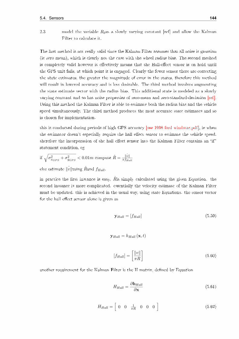
5.4. Sensors 144
2.3 model the variable Rbas a slowly varying constant [ref] and allow the Kalman
Filter to calculate it.
The rst method is not really valid since the Kalman Filter assumes that all noise is gaussian
(ie zero mean), which is clearly not the case with the wheel radius bias. The second method
is completely valid however it eectively means that the Hall-eect sensor is on hold until
the GPS unit fails, at which point it is engaged. Clearly the fewer sensor there are correcting
the state estimates, the greater the magnitude of error in the states, therefore this method
will result in lowered accuracy and is less desirable. The third method involves augmenting
the state estimate vector with the radius bias. This additional state is modeled as a slowly
varying constant and so has noise properties of zero-mean and zero-standard-deviation [ref].
Using this method the Kalman Filter is able to estimate both the radius bias and the vehicle
speed simultaneously. The third method produces the most accurate state estimates and so
is chosen for implementation.
this is conducted during periods of high GPS accuracy [see 1998 ford windstar.pdf], ie when
the estimator doesn't especially require the hall eect sensor to estimate the vehicle speed.
therefore the incorporation of the hall eect sensor into the Kalman Filter contains an if
statement condition, eg
if√σ2xGPS
+ σ2yGPS
< 0.01m compute R =ˆ‖v‖
πfHall
else estimate ˆ‖v‖using Rand fHall.
in practice the rst instance is easy, Ris simply calculated using the given Equation. the
second instance is more complicated. essentially the velocity estimate of the Kalman Filter
must be updated. this is achieved in the usual way, using state Equations. the sensor vector
for the hall eect sensor alone is given as
yHall = [fHall] (5.59)
yHall = hHall (x, t)
[fHall] =[‖v‖πR
](5.60)
another requirement for the Kalman Filter is the H matrix, dened by Equation
HHall =∂hHall∂x
(5.61)
HHall =[
0 0 1πR 0 0 0
](5.62)

145 Chapter 5. State Estimation and Measurement
5.4.3.4 Hall-Effect Sensor Related Tests and Results
5.4.4 Potentiometer
the steering angle sensor is useful as it provides an absolute measure of the vehicle steering
angle (never unavailable).
5.4.4.1 Device Configuration
note that σvpot = σVwiring + σquantisation. σquatisationis dened as:
σquant =∥∥∥∥Vmax − V min
(L− 1)√
12
∥∥∥∥(MSA notes)
Here Vmaxand Vmin are the maximum voltage values output from the pot, and L is the
number of quantisation levels. since the analogue to digital converter card is ????16-bit????
then L = 216. as discussed in the Literature Review, quantisation noise has zero mean and
so may simply be added to the random voltage noise which also has zero mean.
5.4.4.2 Data Decoding Program
5.4.4.3 Integrating the Potentiometer Data into the Kalman Filter
5.5 Recap on the Entire Kalman Filter
5.6 Real Life Results
5.7 Conclusions and Recommendations for Future Work

5.7. Conclusions and Recommendations for Future Work 146
Chapter 6
Control Strategies
The control systems of the TARGET vehicle are all software based applications. These con-
trol strategies, consisting of the Motion Execution and Autonomous Guidance Controllers,
were both developed using Mathworks Matlab and Simulink software. The purpose of the
Autonomous Guidance Controller is to provide steering and speed commands in order for the
vehicle to follow a dened path. The purpose of the Motion Execution Controller is to ensure
that steering and speed commands (given by the Autonomous Control System in autonomous
mode or the handheld controller in RC mode) are implemented onto the vehicle by sending
signals to the vehicle's actuators.
These two controllers have been integrated together along with many other smaller systems
(such as the I/O signals and fault detection systems) in the Onboard Computer Program.
This chapter will discuss the structure and operation of all software components that are run
on the onboard computer system in greater detail.
6.1 Onboard Computer Program
The onboard computer program is the software running on the vehicle's onboard computer.
The program interfaces with various inputs and outputs of the system, integrates the Kalman
Filter, autonomous control, and motion execution control systems together, and performs
mode control and fault monitoring. The program is structured using four main subsystems -
I/O signals, fault detection, mode control, and motor comms. Sound generation is also dis-
cussed in this section despite not being included in the nal program. The onboard computer
program runs at 50Hz, except where specied otherwise. Figure 6.1 shows the top level of the
onboard computer program.
6.1.1 I/O Signals
The I/O signals subsystem is where input and output signals are administered. Input signals
are sampled from peripheral devices, conditioned, and distributed to other parts of the pro-
147

6.1. Onboard Computer Program 148
Figure 6.1: Onboard computer program (top level)

149 Chapter 6. Control Strategies
gram. Output signals are collected and sent to peripheral output devices. There are six types
of input and output (I/O) signals - analogue inputs, counter inputs, digital inputs, digital
outputs, analogue outputs, and RS232 serial communications. These signals are handled by
the peripheral I/O devices discussed in Section 4.2.2.2, which are interfaced to the program
using xPC Target I/O blocks. Figure 6.2 shows the top level of the I/O signals subsystem.
Table 6.1 provides a list of all input and output signals of the system.
Figure 6.2: I/O signals subsystem (top level)
6.1.1.1 Input Signals and Signal Conditioning
The input signals to the program are sampled in the Analogue Inputs, Counter Inputs, and
Digital Inputs subsystems. The analogue and counter inputs are then passed to the Signal
Conditioning subsystem. This subsystem scales the signal to a useful range, and applies
low-pass lters to remove noise. After being conditioned, the signals are distributed around
the program using Goto tags in the blocks titled Get to (analogue, counter, and digital) in.
The Signal Conditioning subsystem treats dierent types of inputs dierently. The analogue
inputs not used for control (battery 1 and 2 levels and current consumption) are ignored.
Analogue inputs that are used for control are scaled to a working range, and low-pass ltered.
These signals are the steering potentiometer, brake pressure transducer, tachometer, and hall
eect speed sensor readings. Scaling for these signals is performed by rst multiplying the
signal by a gain, and then removing a bias. Table 6.2 lists the ranges for each signal after
scaling. Low-pass ltering of the signals is performed using discrete low-pass lters. These
lters were converted from continuous low-pass lters using Tustin's approximation. The
general form of the discrete low-pass lter is shown in Equation (6.1) where τ is the inverse
of the lter's bandwidth.
F (z) =z + 1
z(200τ + 1)− 200τ + 1(6.1)

6.1. Onboard Computer Program 150
Table 6.1: Input and output signals listAnalogue Inputs Board Channel
Battery 1 level PCI-6040E 1
Battery 2 level PCI-6040E 2
Current consumption PCI-6040E 3
Steering potentiometer PCI-6040E 4
Pressure transducer PCI-6040E 5
Tachometer PCI-6040E 6
Hall eect speed sensor PCI-6040E 7
Counter Inputs Board Counter
RC receiver Ch1 - Steering command PCI-6040E 1
RC receiver Ch2 - Speed command PCI-6601 1
RC receiver Ch3 - Gear command PCI-6601 2
RC receiver Ch4 - Ignition command PCI-6601 3
RC receiver Ch5 - Emergency stop command PCI-6601 4
Digital Inputs Board Port/Channel
Capacitive brake sensor PCI-6053 A.1
Transmission position - PARK PCI-6053 A.2
Transmission position - DRIVE PCI-6053 A.3
Transmission position - LOW PCI-6053 A.4
GPS error strobe PCI-6053 A.5
GPS position valid strobe PCI-6053 A.6
Motor running feedback PCI-6053 A.7
Heartbeat pulse from dragon board PCI-6053 A.8
E-brake microswitch PCI-6040E N/A
Digital Outputs Board Port/Channel
Warning light 1 PCI-6053 B.1
Warning light 2 PCI-6053 B.2
Warning light 3 PCI-6053 B.3
Transmission FORWARDS PCI-6053 B.4
Transmission BACKWARDS PCI-6053 B.5
Emergency brake PCI-6053 B.6
Car power PCI-6053 B.7
Starter motor PCI-6053 B.8
Heartbeat pulse to dragon board PCI-6053 C.1
Throttle control 1 PCI-6053 C.2
Throttle control 2 PCI-6053 C.3
Actuator relays PCI-6053 C.4
Analogue Outputs Board Channel
Siren PCI-6040E 1
RS232 Serial Communications Board Port
Roboteq amplier ESC-100 1
Base station computer ESC-100 2
GPS unit ESC-100 3
IMU ESC-100 8
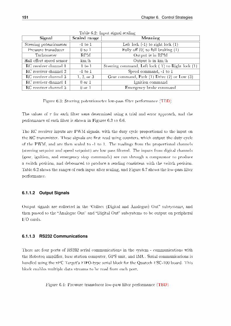
151 Chapter 6. Control Strategies
Table 6.2: Input signal scalingSignal Scaled range Meaning
Steering potentiometer -1 to 1 Left lock (-1) to right lock (1)
Pressure transducer 0 to 1 Fully o (0) to full braking (1)
Tachometer RPM Output is in RPM
Hall eect speed sensor km/h Output is in km/h
RC receiver channel 1 -1 to 1 Steering command, Left lock (-1) to Right lock (1)
RC receiver channel 2 -1 to 1 Speed command, -1 to 1
RC receiver channel 3 1, 2, or 3 Gear command, Park (1) Drive (2) or Low (3)
RC receiver channel 4 0 or 1 Ignition command
RC receiver channel 5 0 or 1 Emergency brake command
Figure 6.3: Steering potentiometer low-pass lter performance (TBD)
The values of τ for each lter were determined using a trial and error approach, and the
performance of each lter is shown in Figures 6.3 to 6.6.
The RC receiver inputs are PWM signals, with the duty cycle proportional to the input on
the RC transmitter. These signals are rst read using counters, which output the duty cycle
of the PWM, and are then scaled to -1 to 1. The readings from the proportional channels
(steering setpoint and speed setpoint) are low-pass ltered. The inputs from digital channels
(gear, ignition, and emergency stop commands) are run through a comparator to produce
a switch position, and debounced to produce a reading consistent with the switch position.
Table 6.2 shows the ranges of each input after scaling, and Figure 6.7 shows the low-pass lter
performance.
6.1.1.2 Output Signals
Output signals are collected in the Collect (Digital and Analogue) Out subsystems, and
then passed to the Analogue Out and Digital Out subsystems to be output on peripheral
I/O cards.
6.1.1.3 RS232 Communications
There are four ports of RS232 serial communications in the system - communications with
the Roboteq amplier, base station computer, GPS unit, and IMU. Serial communications is
handled using the xPC Target's FIFO-type serial block for the Quatech ESC-100 board. This
block enables multiple data streams to be read from each port.
Figure 6.4: Pressure transducer low-pass lter performance (TBD)
6.1. Onboard Computer Program 152
Figure 6.5: Tachometer reading low-pass lter performance (TBD)
Figure 6.6: Hall eect speed sensor low-pass lter performance (TBD)
Roboteq Amplifier Communications
The Roboteq amplier is used to control the steering and brake motors, as discussed in Section
4.8.7. The input to the amplier is an ASCII character string containing information about
the motor command. The message is streamed at 50Hz, chosen to be 10Hz lower than the
maximum rate allowed by the amplier. The output of this port is simply an echo of the
input, which is read at 100Hz and then terminated to prevent FIFO overow error messages.
Base Station Communications
This is the communications link between the base station computer and the onboard computer.
It handles data exchange comprising data to be logged at the base station, control messages
from the base station GUI, and waypoints. Data is sent at 2Hz, as this was found to be the
fastest possible rate at which the base station can receive the data stream. Data is received
at 10Hz, which has been found to be more than adequate for the system.
• Sent data
Data to be sent from the onboard computer to the base station is predominantly for logging
purposes. Logged data mostly comprises measured vehicle states, such as position, speed,
heading, and brake pressure. Other variables transmitted are a heartbeat pulse for monitoring
the RF link, the current control mode of the vehicle, the fault type (if any), and a sound ag
to generate sounds on the base station.
• Control messages
The control messages are inputs from the base station GUI that are used to control the
operation of the vehicle. There are six in total:
1. Control Mode. This species the desired mode of operation of the vehicle, as discussed
in Section 6.1.3.
2. OL or CL Selector. This switches the desired mode of control when in RC mode between
open loop and closed loop, as discussed in Sections 6.1.3 and 6.3.2.
Figure 6.7: RC receiver channels 1 and 2 low-pass lter performance (TBD)
153 Chapter 6. Control Strategies
3. Stop or Go Flag. This acts as both a go button to commence operation of the vehicle,
and as an emergency stop button to halt the vehicle as soon as possible. The go
command is discussed in Section 6.1.3.2, and the emergency stop command is discussed
in Section 6.1.2.2.
4. Heartbeat Pulse. A heartbeat pulse is sent from the onboard computer to the base
station, and is then echoed and sent back to the onboard computer. The pulse is
monitored, and if it stops for more than six seconds the communications loss ag is
taken high.
5. Failure Recover Flag. This ag is taken high to recover the vehicle from failure mode
without requiring re-starting the vehicle, as discussed in Section 6.1.3.4.
6. Connect to Base Station Flag. This ag is taken high when the base station rst connects
to the onboard computer. It is used to prevent any information being sent to the base
station before the base station is ready to accept it; thereby avoiding FIFO overows on
the onboard computer. It is also used to prevent a communications dropout type error
being generated before the base station has connected to the onboard computer. The
implementation of this ag allows the base station, modems, and onboard computer to
be started in any order without generating errors on the onboard computer.
7. Driver Present Flag. This ag is set to 1 to indicate that a driver is present in the vehicle,
and to 2 to indicate that no driver is present. The ag is used to ignore the capacitive
brake sensor when no driver is present, to prevent accidentally entering manual mode
when there is no driver to control the vehicle.
• Waypoints
Waypoints for autonomous control are sent from the base station to the onboard computer,
and stored in a matrix which allows for a maximum of 200 waypoints. The waypoints are
read at 10Hz and are sent from the base station at ????Hz, which ensures that all values are
received. In addition to the waypoints, the base station sends a number which indicates the
total number of waypoints to be sent. This number is used to take a done ag high, which
in turn starts autonomous mode (see Section 6.1.3.2).
GPS Communications
The GPS communications uses a GPS ready ag to handle the order of operation. The order
of operation is as listed in the following section. This method used allows for a completely
non-specic start-up order of the system.
• Power-on

6.1. Onboard Computer Program 154
The GPS is powered from the electronics board that is turned on at the commencement of
initialisation mode (see Section 6.1.3). The unit is ready to receive a log command approx-
imately 10 seconds after being turned on. When it is ready, the GPS unit sends the ASCII
message [COM1].
• GPS ready
The onboard computer initially uses an ASCII read block to read [COM1] message. When it
is received, the GPS ready ag is set high.
• Log command and binary read
The GPS ready ag is used to both send a log command, and change the read method. On
a rising edge of the ag, the ASCII message log bestxyzb ontime 0.1\r is sent once. This
commands the GPS to send a binary type log of position data at 10Hz. When the GPS ready
ag is high, the ASCII read block used to search for the [COM1] message is disabled, and a
binary read block used to read the GPS log is enabled.
IMU Communications
The IMU communications is straightforward. On receiving a command message, the IMU
returns a log in the form of a vector of bytes. The command message is sent at 20Hz, and
data is also received at this rate.
6.1.2 Fault Detection
Fault detection is performed as a safety precaution, to determine when a potentially hazardous
fault in the system has occurred. Faults monitored predominantly comprise hardware and
communications failures. The fault detection routine initially passes all of the continuous
input signals (analogue and PWM duty cycle readings) through a rate and range checker.
Other faults are also collected from various parts of the program. The output of the rate and
range checker is placed along with the other faults onto a vector. This vector is nally passed
through the fault nder, to produce the output variables fault ag and fault type. Table
6.3 lists all of the faults monitored by the program. Figure 6.8 shows the top level of the fault
detection subsystem.

155 Chapter 6. Control Strategies
Table 6.3: Faults monitored by onboard computerFault
NumberFault name Description
1 Battery 1 level range Sensor reading out of desired range
2 Battery 2 level range Sensor reading out of desired range
3 Current consumption range Sensor reading out of desired range
4 Steering potentiometer range Sensor reading out of desired range
5 Pressure transducer range Sensor reading out of desired range
6 Tachometer range Sensor reading out of desired range
7 Hall eect speed sensor range Sensor reading out of desired range
8 RC receiver Ch.1 range Sensor reading out of desired range
9 RC receiver Ch.2 range Sensor reading out of desired range
10 RC receiver Ch.3 range Sensor reading out of desired range
11 RC receiver Ch.4 range Sensor reading out of desired range
12 RC receiver Ch.5 range Sensor reading out of desired range
13 Battery 1 level rate Sensor reading exceeding desired rate limit
14 Battery 2 level rate Sensor reading exceeding desired rate limit
15 Current consumption rate Sensor reading exceeding desired rate limit
16 Steering potentiometer rate Sensor reading exceeding desired rate limit
17 Pressure transducer rate Sensor reading exceeding desired rate limit
18 Tachometer rate Sensor reading exceeding desired rate limit
19 Hall eect speed sensor rate Sensor reading exceeding desired rate limit
20 RC receiver Ch.1 rate Sensor reading exceeding desired rate limit
21 RC receiver Ch.2 rate Sensor reading exceeding desired rate limit
22 RC receiver Ch.3 rate Sensor reading exceeding desired rate limit
23 RC receiver Ch.4 rate Sensor reading exceeding desired rate limit
24 RC receiver Ch.5 rate Sensor reading exceeding desired rate limit
25 Emergency stop activation (GUI) Emergency stop request from base station computer
26 GPS error strobe assertion GPS hardware failure
27 Kalman lter type error Error reported from Kalman lter
28 Modem communication dropout RF link with base station computer failure
29 RC communications loss RC communications loss
30 Emergency stop activation (RC) Emergency stop request from RC transmitter
31 Heartbeat failure (dragon) Heartbeat pulse from dragon board failure
32 Multiple simultaneous faults Multiple simultaneous faults present in system
Figure 6.8: Fault detection subsystem top level

6.1. Onboard Computer Program 156
6.1.2.1 Range and Rate Checker
The range and rate checker monitors the rate and range of the continuous input signals.
These signals are the analogue inputs and the PWM duty cycle values. The output of the
rate and range checker is a vector, with two elements for each signal monitored. One of these
elements is taken high if the signal is outside its desired static range, and the other element
is taken high if the signal is moving faster than its maximum desired rate. Signals must be
outside their static range limit for more than ten time steps to produce a range error. Signals
produced by the RC receiver are not monitored unless the desired operation mode is set to
RC by the base station user. The range and rate errors comprise entries 1 to 24 of Table 6.3.
6.1.2.2 Other Faults
The subsystem Other faults collects eight ags from other parts of the program indicating
faults. These faults are listed in entries 25 to 31 of Table 6.3. The Other faults subsystem
also includes a routine for detecting a loss of RC communications.
• Fault 25 - Emergency Stop Activation (GUI)
This fault is generated when the emergency stop button is pressed by the user on the base
station computer.
• Fault 26 - GPS error strobe
The GPS error strobe is a digital output of the GPS unit. The strobe is taken high in the
event of a hardware failure.
• Fault 27 - Kalman Filter type error
The Kalman Filter includes its own routine for monitoring faults. If the Kalman Filter detects
a critical fault, a Kalman Filter type error is generated.
• Fault 28 - Modem communication dropout
This fault is generated if the heartbeat pulse sent from the base station to the onboard
computer is inactive for more than six seconds.
• Fault 29 - RC communications loss

157 Chapter 6. Control Strategies
This fault is generated when RC communications are oine, and is discussed in greater detail
later in this section.
• Fault 30 - Emergency stop activation (RC)
This fault can be generated by the user pressing the emergency stop activation switch on the
RC transmitter.
• Fault 31 - Dragon board heartbeat failure
The dragon board is linked to the onboard computer by a two-way heartbeat pulse. This
pulse is monitored on both ends. If the onboard computer detects that the heartbeat pulse
generated by the dragon board has stopped, a fault ag is set high.
• Fault 32 - Multiple simultaneous faults
This fault is generated when multiple faults occur in a single time step. Using this fault allows
the output of the fault detection system to be a scalar whose value corresponds to a specic
fault type.
6.1.2.3 RC Communications Loss Monitoring
The Other faults subsystem includes a routine for monitoring RC communications. This
routine exploits the fact that when the RC receiver cannot detect a transmitted signal, its
output is completely static. The communications loss monitor requires that the output of the
receiver is static for at least twenty time steps. There are two outputs of this routine. The
rst is a ag to indicate that RC communications have failed while the vehicle is in RC mode.
This output is treated as a fault. The second output of the routine is a ag to indicate that
RC communications are operating normally (RC comms OK). The RC comms OK ag is used
along with the emergency stop activation from the RC transmitter to determine if it is appro-
priate to generate a fault; i.e. a fault can be generated from the RC transmitter regardless of
the mode of operation, providing that RC communications are operating normally.
6.1.2.4 Fault Finder
The fault nder monitors the ags produced by the range and rate checker and by the other
faults subsystem. There are two outputs - fault ag and fault type. The fault ag is taken
high whenever any of the previously discussed faults occurs, and the fault type is a scalar
whose value corresponds to one of the faults. The fault ag is used by the mode chart, to
determine when failure mode must be activated. The fault type variable is latched to the
current fault each time the fault ag goes high. Its value is shown by the fault type entry
in Table 6.3.
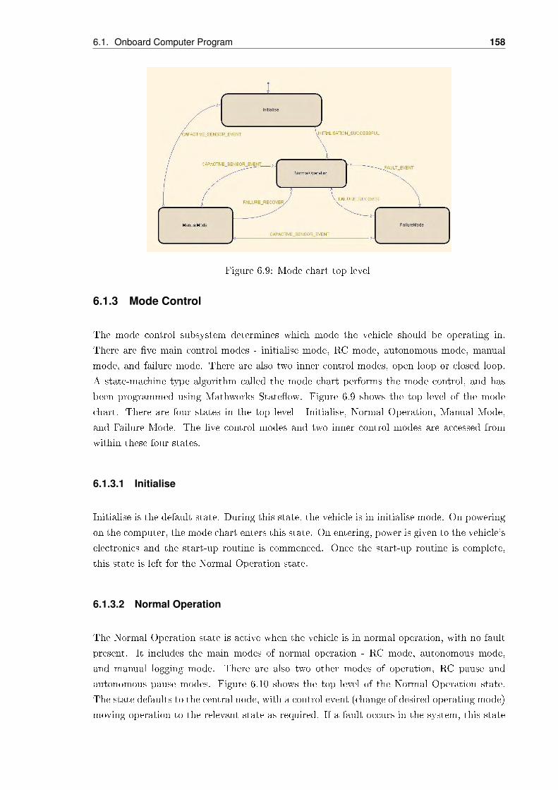
6.1. Onboard Computer Program 158
Figure 6.9: Mode chart top level
6.1.3 Mode Control
The mode control subsystem determines which mode the vehicle should be operating in.
There are ve main control modes - initialise mode, RC mode, autonomous mode, manual
mode, and failure mode. There are also two inner control modes, open loop or closed loop.
A state-machine type algorithm called the mode chart performs the mode control, and has
been programmed using Mathworks Stateow. Figure 6.9 shows the top level of the mode
chart. There are four states in the top level - Initialise, Normal Operation, Manual Mode,
and Failure Mode. The ve control modes and two inner control modes are accessed from
within these four states.
6.1.3.1 Initialise
Initialise is the default state. During this state, the vehicle is in initialise mode. On powering
on the computer, the mode chart enters this state. On entering, power is given to the vehicle's
electronics and the start-up routine is commenced. Once the start-up routine is complete,
this state is left for the Normal Operation state.
6.1.3.2 Normal Operation
The Normal Operation state is active when the vehicle is in normal operation, with no fault
present. It includes the main modes of normal operation - RC mode, autonomous mode,
and manual logging mode. There are also two other modes of operation, RC pause and
autonomous pause modes. Figure 6.10 shows the top level of the Normal Operation state.
The state defaults to the central node, with a control event (change of desired operating mode)
moving operation to the relevant state as required. If a fault occurs in the system, this state

159 Chapter 6. Control Strategies
is left for Failure Mode. Similarly, if the capacitive brake sensor is pressed, this state is left
for Manual Mode.
• RC mode
During RC mode, the vehicle is controlled by the handheld RC transmitter. During RC mode
the inner control mode can be changed between open loop and closed loop at any time, by
pressing a button on the base station computer.
• Autonomous mode
During autonomous mode, the vehicle is controlled by waypoints entered on the base station
computer. The inner control mode is set to speed control, as required by the autonomous
control system.
• Manual logging mode
Manual logging mode can be activated if the user wishes to drive the vehicle manually, when
not in an emergency situation. The primary purpose for this is to drive a test path, which is
logged, and then reproduced as waypoints for autonomous operation. During this mode all
actuators are turned o to give the user full control of the vehicle.
• RC pause and autonomous pause modes
When RC mode or autonomous mode is activated, the mode initially defaults to RC pause
or autonomous pause mode. In the pause mode the respective mode is activated, but the
vehicle is unable to move until the 'Go' button is pressed on the base station computer. This
prevents sudden and unpredictable vehicle operation when users are not ready. Autonomous
mode pause mode will also be activated until a done ag is received indicating that all
waypoints have been received, see Section 6.1.1.3.
6.1.3.3 Manual Mode
This state is always entered when the capacitive brake sensor is pressed. In this state, manual
mode is active. This mode is a safety precaution, which allows a driver to take control of the
vehicle at any time. During this mode all actuators are turned o to give the user full control
of the vehicle. Manual mode is not left unless the failure recover button is pressed on the
base station computer. This mode diers from manual logging mode only in the conditions
for entering and leaving.

6.1. Onboard Computer Program 160
Figure 6.10: Normal Operation state top level
6.1.3.4 Failure Mode
This state is entered when the vehicle is in one of the normal modes of operation (RC,
autonomous, or manual logging mode), and the fault ag is asserted. Entering this mode
causes the throttle to be released, brakes set to 75% pressure, and steering wheel latched to
its last position. After eight seconds of Failure Mode, the emergency brake system is activated
(see Section ??) to stop the vehicle in the case of a braking system failure. Once the vehicle
is stopped, the transmission is put into park, and nally the vehicle is turned o. Failure
Mode is left for Normal Operation if the failure recover button is pressed on the base station
computer.
6.1.3.5 Inner Control Mode
In addition to the modes of operation discussed previously, the vehicle can be set to operate
in closed loop or open loop mode. During closed loop mode, the throttle and brake actuators
are used alternately to make the vehicle follow a desired speed. Closed loop mode is always
active in autonomous mode, and can be set to active in RC mode. During open loop mode,
the speed command provides open loop control of the cruise control unit (when the command
is greater than 1) and pressure control of the brake actuator (when the command is less than
1). Open loop mode is always active during failure mode and initialise mode, and can be set
to active in RC mode.
6.1.4 Motor Comms
The motor comms subsystem handles communications with the various actuators in the system
- the steering and brake motors, the cruise control unit, transmission motor, and ignition. This

161 Chapter 6. Control Strategies
subsystem takes actuator commands from the motion execution control system, and converts
these commands into the format required by the actuators.
6.1.4.1 Steering and Brake Motors
The steering and brake motors are controlled by the Roboteq amplier via RS232 serial
communications. A desired speed for each of these motors enters the motor comms subsystem
as a value from -1 to 1. This command is then converted to the ASCII string required by the
Roboteq amp using an embedded m-le.
6.1.4.2 Cruise Control Unit
The cruise control unit has three inputs - an inlet valve, outlet valve, and dump. The dump
is not controlled by the computer, and is discussed in Sections 8.1.2 and 4.8.2. The inlet and
outlet valves are controlled by digital outputs of the onboard computer. By manipulating the
inlet and outlet valves, the throttle can be moved either in (increase throttle), out (decrease
throttle), or held in place. The unit is operated as follows:
• To increase throttle, the inlet valve is open and the outlet closed.
• To decrease throttle the inlet valve is closed and the outlet valve is open.
• To hold the throttle in place both valves are held closed.
The throttle control routine receives a command between -1 and 1, where -1 releases the
throttle at full speed and 1 increases the throttle at full speed. The routine generates a
PWM whose duty cycle is proportional to the magnitude of the command. This PWM is
used to switch between increasing or decreasing the throttle (depending on the sign of the
command), and holding it still. This approach allows the throttle to be moved at a variable
rate, depending on the magnitude of the command. The throttle control routine is run at
100Hz to achieve adequate resolution of the control signal.
6.1.4.3 Transmission Control
Control of the vehicle's transmission is achieved using a bang-bang (on-o) style approach.
The transmission control routine is capable of moving the transmission motor either forwards
or backwards using digital outputs. The routine uses feedback on the transmission position
to determine whether to move the transmission forwards, backwards, or not at all. There is
also a speed input to the routine, which is used to prevent changing gears unless the speed of
the vehicle is very low. A required speed for gear changing of zero could not be used as the
Kalman Filter will never return a speed of exactly zero.

6.1. Onboard Computer Program 162
6.1.4.4 Ignition Control
Ignition control is achieved using a command from either the mode chart when in autonomous
mode, or from the RC transmitter when in RC mode. When the command is received, the
starter motor digital output is taken high until the program receives feedback that the engine
has started.
6.1.5 Startup Routine
Succesful operation of the TARGET vehicle relies on all actuators, sensors and communica-
tions equipment operating as expected. To check that these systems are operating as required
prior to testing, an automated startup routine has been implemented. The startup routine
carries out a series of tests which are listed in the following points, and are executed in the
numbered order:
1. Ensure the vehicle transmission is in park
2. Check that the communications are working by sending and then receiving data
3. Check a ag from the GPS to ensure it is in working order
4. Check a ag from the IMU to ensure it is in working order
5. Get a user to place their foot on the brake to ensure the capacitive sensor is operational
6. Move the transmission lever from park to drive and back again
7. Start the vehicle ignition
8. Test that the brake pressure transducer feedback is in an acceptable range
9. Test that the steering potentiometer feedback is in an acceptable range
10. Test the steering by moving it to its limits, then returning to the center position
11. Ensure the brake actuator is operational by applying the brakes
12. Test the throttle using feedback from the tachometer
When all of these tests have been performed succesfully the vehicle is able to be operated.
However, if errors are found in the system testing cannot commence untill these errors are
resolved, and the startup routine has been completed succesfully.
The startup routine has been implemented using the Stateow package of Simulink. The
highest level of the startup routine Stateow program is shown in Figure 6.11. The startup
routine consists of two states at the highest level , which are 'STARTUP' and 'STOP'. The
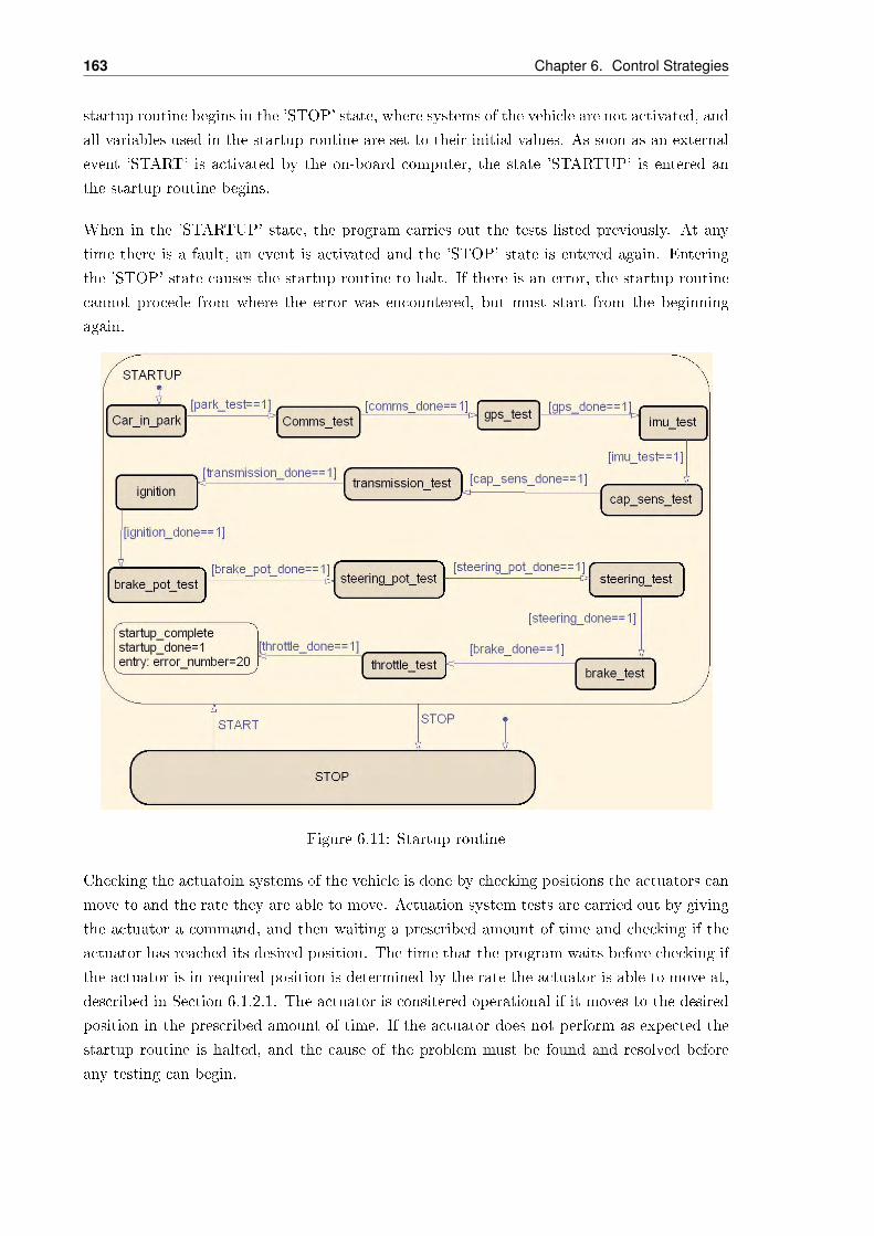
163 Chapter 6. Control Strategies
startup routine begins in the 'STOP' state, where systems of the vehicle are not activated, and
all variables used in the startup routine are set to their initial values. As soon as an external
event 'START' is activated by the on-board computer, the state 'STARTUP' is entered an
the startup routine begins.
When in the 'STARTUP' state, the program carries out the tests listed previously. At any
time there is a fault, an event is activated and the 'STOP' state is entered again. Entering
the 'STOP' state causes the startup routine to halt. If there is an error, the startup routine
cannot procede from where the error was encountered, but must start from the beginning
again.
Figure 6.11: Startup routine
Checking the actuatoin systems of the vehicle is done by checking positions the actuators can
move to and the rate they are able to move. Actuation system tests are carried out by giving
the actuator a command, and then waiting a prescribed amount of time and checking if the
actuator has reached its desired position. The time that the program waits before checking if
the actuator is in required position is determined by the rate the actuator is able to move at,
described in Section 6.1.2.1. The actuator is consitered operational if it moves to the desired
position in the prescribed amount of time. If the actuator does not perform as expected the
startup routine is halted, and the cause of the problem must be found and resolved before
any testing can begin.
6.2. Autonomous Guidance Control 164
6.1.6 Sound Generation
The TARGET vehicle includes a siren intended for playing warning messages. Two techniques
for generating sounds using the onboard computer have been developed, but unfortunately
have not been included in the nal program due to the demanding amount of processing
power required. The most promising technique is discussed here, and is included in smaller
versions of the program such as the one that will be running during the project exhibition.
Both methods of sound generation are discussed in greater detail in Appendix A.
The most promising method of sound generation involves reading a stored sound data le from
the onboard computer's hard drive, and playing the sound as an analogue output driving the
vehicle's siren. The sounds are rst read in Matlab from a wave le recorded at 8kHz. They
are then put into a single data le in matrix form, with each row corresponding to a single
sound. Multiple les cannot be used, as xPC Target can only handle eight individual les.
To play a sound, all rows of this data le are read at 8kHz, and a single row is selected and
written to the analogue output device at each time step. This method requires too much
processing power to run along with the rest of the program, and therefore sound generation
has been excluded.
6.2 Autonomous Guidance Control
Autonomous guidance control forms the high level decision-making control in the TARGET
vehicle system and is responsible for ensuring that the autonomous vehicle is able to safely,
accurately, smoothly, rapidly and consistently follow a desired waypoint-dened path. The
autonomous guidance control has been implemented as an embedded software component of
the vehicle's onboard computer, and is executed in real time during the vehicle's autonomous
operation.
The Autonomous Guidance Controller essentially determines the appropriate vehicle motion,
in the form of steering angle and speed setpoints. This vehicle motion decision is based on
a comparison of the current vehicle information obtained from the Kalman Filter (actual
vehicle position and heading) and the path waypoints commanded from a remote base station
computer (describing desired vehicle position and speed). A diagram depicting the general
ow of the overall autonomous control system and the centralised role of the Autonomous
Guidance Controller is presented in Figure 6.12.
In autonomous mode, an operator at a remote base station computer enters a desired path
into a graphical user interface (GUI), as described in detail in Chapter 7. This path is
converted into multiple waypoints that are wirelessly transmitted to the vehicle's onboard
computer via Radio Frequency (RF) modems. The complete list of waypoints is supplied to
the Autonomous Guidance Controller together with the current vehicle state estimates (vehicle
position and heading) acquired from the Kalman Filter following its fusion of various sensor

165 Chapter 6. Control Strategies
Figure 6.12: General autonomous control ow

6.2. Autonomous Guidance Control 166
data. The Autonomous Guidance Controller then determines the appropriate vehicle driving
commands (steering angle and speed) in the interest of achieving optimal path tracking, and
these commands are executed by the Motion Execution Controller which controls the vehicle
actuators in order to achieve the desired steering, acceleration and / or braking behaviour.
The autonomous guidance control task is closely linked to the following specic project goals:
• Derive an accurate mathematical model of the relevant vehicle dynamics
• Achieve successful autonomous control of the TARGET vehicle
• Enable intelligent and safe switching between normal human driving, remote control
and autonomous modes of operation
The detailed exposition of the Autonomous Guidance Control presented in Section 6.2 de-
scribes the autonomous steering and speed guidance strategies, explains the structure of the
controller and associated control parameter calculations, and discusses the simulation and
tuning of the controller and the required mathematical vehicle model.
6.2.1 Autonomous Guidance Control Strategy
The Autonomous Guidance Controller comprises the two separate but related functions of
vehicle steering and speed guidance control, with steering guidance responsible for generating
a steering angle command, and speed guidance responsible for generating a vehicle speed
command, both of which are in the interest of achieving optimal and safe path tracking
performance.
This section will deconstruct the overall autonomous guidance control strategy into its sepa-
rate steering and speed guidance components, but before launching into this detailed discus-
sion it is rst necessary to outline the general control environment and reference structures.
For the purpose of autonomous guidance control, the TARGET vehicle is considered to be
located on a 2D spatial plane designated by the coordinate axes of Easting, E (or metres
East), and Northing, N (or metres North), as indicated in Figure 6.13.
Relative to this coordinate plane, the vehicle can be described by its position, [Ev, Nv], as
dened at the midpoint of the rear axle; heading, θv, dened as the vehicle orientation relative
to East; and steering angle, φ, as dened relative to the forward centreline axis of the vehicle.
The path waypoints sent from the remote base station computer, [Ew, Nw, vw], each contain a
desired vehicle position, [Ew,Nw], and a desired vehicle speed, vw. The Autonomous Guidance
Controller interprets the waypoints as being connected by straight line segments to form a
piece-wise continuous path. Each straight line connecting a pair of consecutive waypoints is
known as a path segment. Although curved line segments would have yielded a smoother path,
they would have also severely increased the diculty of the control parameter calculations

167 Chapter 6. Control Strategies
Figure 6.13: Autonomous control environment
(see Section 6.2.2.1) and placed a signicantly greater load on the vehicle's real-time onboard
computer system.
Having designated the autonomous control environment and reference structure, the discussion
will now progress to the specic control strategies used in steering and speed guidance control,
beginning with steering guidance.
6.2.1.1 Steering Guidance Strategy
The steering guidance uses the general principles of a spatial control technique known as the
Virtual Vehicle Approach to produce the required steering angle setpoint. While there are
many variations of this path tracking control technique (Egerstedt et al., 2001; Barton, 2001),
the Virtual Vehicle Approach basically compares the vehicle to a continuously updated path
reference point and its associated path segment. This continuously updated path reference
point is called the virtual vehicle point, and is dened as the closest point on the path to
the current vehicle position (that is, the position of the midpoint of the vehicle's real axle)
such that a line drawn between the virtual vehicle point and the vehicle position would be
perpendicular to the path. Referring to Figure 6.13, the virtual vehicle path segment is
highlighted in orange, while the virtual vehicle point is portrayed in red. This autonomous
guidance control technique is called the Virtual Vehicle Approach because the reference point,
which moves along the path as the real vehicle moves, is a virtual representation of the ideal
motion of the vehicle. Hence, if the vehicle were to follow the path perfectly, the vehicle's
position would at all times coincide with the virtual vehicle point.
With reference to the Literature Review in Section 3.5.2.1, the Virtual Vehicle Approach was
selected as the foundational strategy of the guidance controller because it had demonstrated

6.2. Autonomous Guidance Control 168
strong path-tracking potential a relatively accessible / ecient (as opposed to arduous) design
ow. Fuzzy control was also originally considered on a similar basis, but in order to provide
eective guidance for the complex nature of vehicle behaviour, this strategy would have placed
a signicantly greater burden on the vehicle's real-time onboard computer system.
Using the principles of the Virtual Vehicle Approach (Barton, 2001), the steering guidance
incorporates three control parameters:
1. Cross-track error, d⊥
2. Heading error, θe
3. Projected steering angle, φproj
The rst steering guidance control parameter, cross-track error, d⊥, is the perpendicular
distance (measured in metres) between the virtual vehicle point and the actual vehicle position,
and hence gives a measure of the position error (between the desired and actual vehicle
position). By minimising the cross-track error the controller returns the vehicle to the desired
path.
The second control parameter, heading error, θe (measured in degrees), is the dierence be-
tween the orientation of the virtual vehicle path segment and the vehicle heading, both mea-
sured relative to East. By minimising the heading error the controller seeks to align the
vehicle heading with the path orientation. If properly tuned, this causes the vehicle to ap-
proach the path asymptotically rather than simply guiding the vehicle directly towards the
virtual vehicle point which can lead to signicant overshoot.
The third steering guidance control parameter, projected steering angle, φproj , is the approx-
imate steering angle (measured in degrees) required to track the average curvature of an
upcoming number of path segments (refer to Section 6.2.2.1 for the mathematical denition).
The steering guidance controller uses this control parameter to anticipate corners and adjust
the vehicle steering angle accordingly. Whilst the cross-track error and heading error are
purely reactive control parameters, that is they only produce control action once the vehi-
cle has actually deviated from the desired path (in terms of position and orientation), the
projected steering angle term adds an important feedforward element to the controller which
eectively helps the TARGET vehicle to track the curvature of the path without actually
deviating from it.
Thus the steering angle setpoint generated by the steering guidance control is a function of
the cross-track error, heading error, and projected steering angle. For the mathematical de-
nition and calculation of these steering guidance control parameters, the reader is referred to
Section 6.2.2.1. The other side to the autonomous guidance control strategy, speed guidance,
will now be discussed.

169 Chapter 6. Control Strategies
6.2.1.2 Speed Guidance Strategy
The speed guidance component of the TARGET vehicle's autonomous guidance control system
also uses the general principles of the Virtual Vehicle Approach, but in a more liberal fashion.
A lack of engagement with speed guidance concepts in the available academic literature led
to the need for some creativity in the development of the TARGET's speed guidance control.
Like the steering guidance control, the speed guidance uses three control parameters to pro-
duce an appropriate vehicle speed setpoint:
1. Desired speed, vw, as dened in the waypoints
2. Projected curvature, κproj
3. Cross-track error, d⊥
A ow diagram of the speed guidance control scheme is shown in Figure 6.14.
The desired speed, vw, dened in the waypoints provides the benchmark speed that the guid-
ance controller seeks to attain in the autonomous vehicle. Nevertheless, in the interests of
safety and eective path-tracking, it is also desirable to have some intelligent backup speed
reduction mechanisms in place that are able to automatically reduce the vehicle speed to an
appropriate level in particular circumstances, such as when the vehicle is approaching a rel-
atively sharp corner or signicantly deviating from the desired path. Essentially, the desired
vehicle speed dened in the waypoints forms the vehicle speed setpoint unless the projected
curvature or cross-track error lead to a slower speed recommendation.
The projected curvature, κproj , which is the average curvature across a number of upcoming
path segments (and is therefore related to the aforementioned projected steering angle), is
used to produce an alternative speed recommendation called the approach speed, which is
based on maintaining a comfortable lateral acceleration of 0.3g (see Section 6.2.2.2). This
alternative speed recommendation forms the basis for the autonomous speed setpoint if it is
slower than the speed specied in the waypoints. This control mechanism helps to prevent
the vehicle from overshooting sharp corners due to excessive speed.
The speed guidance controller thus selects the slower of the two recommended speeds (that
is, either the desired speed dened in the waypoints and the recommended approach speed
determined from the projected curvature) and this recommended speed is then multiplied
and eectively ltered by a function related to the cross-track error, which is the third speed
guidance control parameter. The logic behind this lter function is that the vehicle should
experience a decrease in speed proportional to its deviation (cross-track error) once it has
drifted from the path beyond an allowable bound. This behaviour is desirable both as a safety
precaution, since the vehicle will ultimately stop once it has deviated beyond a maximum limit,
and as a control feature, since slowing the vehicle down allows the controller more time to
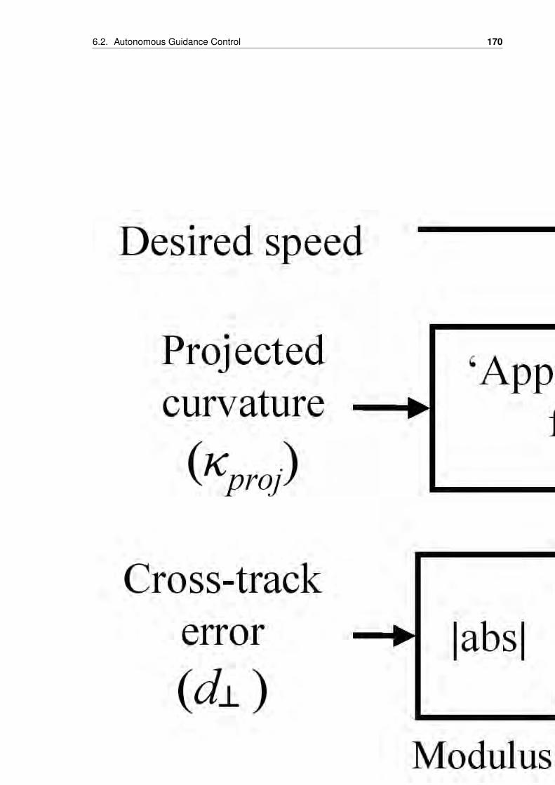
6.2. Autonomous Guidance Control 170
Figure 6.14: Speed guidance control scheme
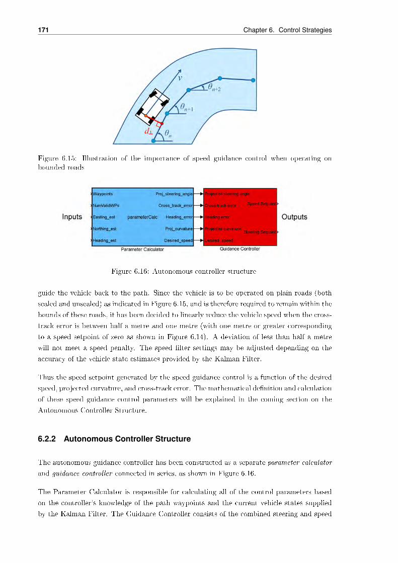
171 Chapter 6. Control Strategies
Figure 6.15: Illustration of the importance of speed guidance control when operating onbounded roads
Figure 6.16: Autonomous controller structure
guide the vehicle back to the path. Since the vehicle is to be operated on plain roads (both
sealed and unsealed) as indicated in Figure 6.15, and is therefore required to remain within the
bounds of these roads, it has been decided to linearly reduce the vehicle speed when the cross-
track error is between half a metre and one metre (with one metre or greater corresponding
to a speed setpoint of zero as shown in Figure 6.14). A deviation of less than half a metre
will not meet a speed penalty. The speed lter settings may be adjusted depending on the
accuracy of the vehicle state estimates provided by the Kalman Filter.
Thus the speed setpoint generated by the speed guidance control is a function of the desired
speed, projected curvature, and cross-track error. The mathematical denition and calculation
of these speed guidance control parameters will be explained in the coming section on the
Autonomous Controller Structure.
6.2.2 Autonomous Controller Structure
The autonomous guidance controller has been constructed as a separate parameter calculator
and guidance controller connected in series, as shown in Figure 6.16.
The Parameter Calculator is responsible for calculating all of the control parameters based
on the controller's knowledge of the path waypoints and the current vehicle states supplied
by the Kalman Filter. The Guidance Controller consists of the combined steering and speed
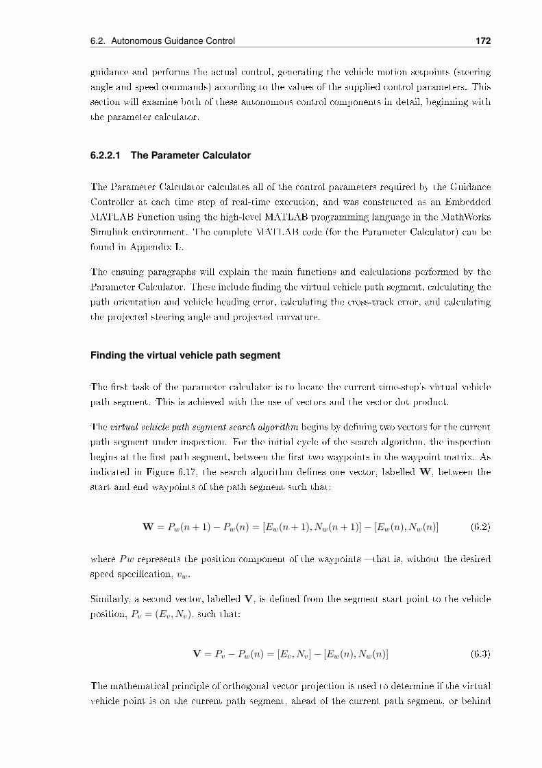
6.2. Autonomous Guidance Control 172
guidance and performs the actual control, generating the vehicle motion setpoints (steering
angle and speed commands) according to the values of the supplied control parameters. This
section will examine both of these autonomous control components in detail, beginning with
the parameter calculator.
6.2.2.1 The Parameter Calculator
The Parameter Calculator calculates all of the control parameters required by the Guidance
Controller at each time step of real-time execution, and was constructed as an Embedded
MATLAB Function using the high-level MATLAB programming language in the MathWorks
Simulink environment. The complete MATLAB code (for the Parameter Calculator) can be
found in Appendix L.
The ensuing paragraphs will explain the main functions and calculations performed by the
Parameter Calculator. These include nding the virtual vehicle path segment, calculating the
path orientation and vehicle heading error, calculating the cross-track error, and calculating
the projected steering angle and projected curvature.
Finding the virtual vehicle path segment
The rst task of the parameter calculator is to locate the current time-step's virtual vehicle
path segment. This is achieved with the use of vectors and the vector dot product.
The virtual vehicle path segment search algorithm begins by dening two vectors for the current
path segment under inspection. For the initial cycle of the search algorithm, the inspection
begins at the rst path segment, between the rst two waypoints in the waypoint matrix. As
indicated in Figure 6.17, the search algorithm denes one vector, labelled W, between the
start and end waypoints of the path segment such that:
W = Pw(n+ 1)− Pw(n) = [Ew(n+ 1), Nw(n+ 1)]− [Ew(n), Nw(n)] (6.2)
where Pw represents the position component of the waypoints that is, without the desired
speed specication, vw.
Similarly, a second vector, labelled V, is dened from the segment start point to the vehicle
position, Pv = (Ev, Nv), such that:
V = Pv − Pw(n) = [Ev, Nv]− [Ew(n), Nw(n)] (6.3)
The mathematical principle of orthogonal vector projection is used to determine if the virtual
vehicle point is on the current path segment, ahead of the current path segment, or behind

173 Chapter 6. Control Strategies
Figure 6.17: Virtual vehicle search vectors
Figure 6.18: Virtual vehicle point located behind current path segment
the path segment, by considering the orthogonal projection of the waypoint-to-vehicle vector
V onto the path segment vector W.
The orthogonal projection of V onto W is given by the equation:
|V| cos(α) =W •V|W|
(6.4)
where the vector dot product:
W •V = [w1, w1] • [v1, v2] = w1× v1 + w2× v2 (6.5)
Following from these relationships it can be shown that W •V < 0 implies that the projection
of V onto W extends backwards behind the start waypoint of the current path segment as
indicated in Figure 6.18, and hence the search algorithm must look behind the current path
segment in order to nd (or at least get closer to) the virtual vehicle point.

6.2. Autonomous Guidance Control 174
Figure 6.19: Virtual vehicle point located beyond current path segment
Otherwise, if W •V > 0 and V •V < V •W, then the projection of V onto W extends
beyond the current path segment as shown in Figure 6.19, and hence the search algorithm
must look beyond the current path segment in order to nd the virtual vehicle point.
Thus the search algorithm appropriately increments or decrements through the path segments
until the virtual vehicle path segment is discovered. This occurs when neither W •V > 0 nor
V •V < V •W is true for the current path segment, indicating that the projection of V onto
W, and hence the virtual vehicle point, is between the segments start and end waypoints.
Some additional logic has been included to handle the special case of autonomously negotiating
a closed circuit path, for which the beginning and end waypoints are connected. In this
situation, the last segment precedes the rst segment, and the rst segment follows on from
the last segment.
There are also some situations, such as the one indicated in Figure 6.20, when the vehicle (and
hence the projection of V onto W) is between path segments. In this case, the forward of the
two segments is treated as the virtual vehicle path segment, and this segment is eectively
extended to the virtual vehicle point. Similarly, if the vehicle starts behind the rst waypoint
in an open path, for which the beginning and end waypoints do not share the same location,
the rst path segment is treated as the virtual vehicle segment and extended back to the
virtual vehicle point. It should be noted that for both open and closed circuit paths, the
initial virtual vehicle path segment is not necessarily the rst path segment in the specied
path but approximately the closest path segment to the vehicle's starting position.
The virtual vehicle path segment search algorithm is an application and expansion of the
equations and algorithms described in Mörtberg (2006), Sunday (2006) and Kreyszig (1999).
Calculating the path orientation and vehicle heading error
Once the virtual vehicle path segment has been found, the guidance control parameters that
were introduced in Section 6.2.1 can begin to be calculated. These control parameters include
the vehicle heading error used in steering guidance.

175 Chapter 6. Control Strategies
Figure 6.20: Vehicle located between path segments
The heading error, θe (measured in degrees), is the dierence between the orientation of the
virtual vehicle path segment and the vehicle heading, both measured relative to East. Thus,
with reference to Figure 6.13, the heading error is given by:
θe = θn + θv (6.6)
Which follows the generic form:
error = desired value − actual value (6.7)
The vehicle heading, θv, is supplied by the Kalman Filter via GPS and IMU measurements
(see Chapter 5), but the orientation of the virtual vehicle path segment, θn, is calculated using
the following equation, with reference to Figure 6.21:
θn = arctan(y step
x step
)= arctan
(Nw(n+ 1)−Nw(n)Ew(n+ 1)− Ew(n)
)(6.8)
The heading error can then be calculated using Equation (6.8) to give values in the range
−180 < θe < 180, but manipulated such that a negative heading error corresponds to the
vehicle moving towards the left of the track, and a positive heading corresponds to the vehicle
moving towards the right of the track. Note that the left and right directions are referenced
according to the vehicle's perspective.

6.2. Autonomous Guidance Control 176
Figure 6.21: Determining the orientation of the virtual vehicle path segment
Figure 6.22: Calculating the cross-track error, d⊥
Calculating the cross-track error
The cross-track error control parameter is required for both the steering and speed compo-
nents of autonomous guidance control. Recall that the cross-track error is dened as the
perpendicular distance (measured in metres) between the virtual vehicle point and the actual
vehicle position.
Using the two vectors established in the virtual vehicle search algorithm as shown in Fig-
ure 6.22, the cross-track error calculation process is initiated by evaluating the orthogonal
projection of V onto W to determine the distance from the start waypoint of the virtual
vehicle path segment to the virtual vehicle point using the previously stated Equation (6.9):
dvv = |V| cos(α) =W •V|W|
(6.9)
The parametric equation of a line (Sunday, 2006) is then used to determine the location of the
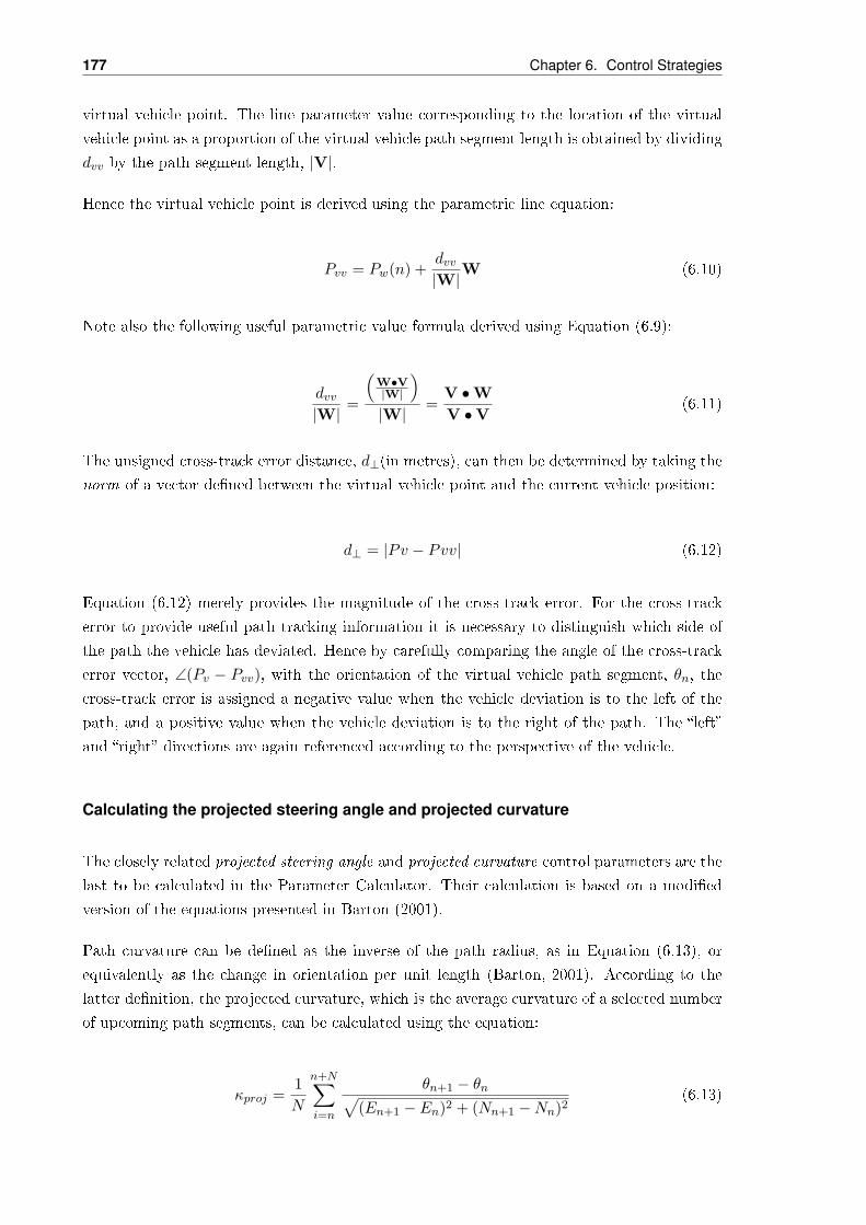
177 Chapter 6. Control Strategies
virtual vehicle point. The line parameter value corresponding to the location of the virtual
vehicle point as a proportion of the virtual vehicle path segment length is obtained by dividing
dvv by the path segment length, |V|.
Hence the virtual vehicle point is derived using the parametric line equation:
Pvv = Pw(n) +dvv|W|
W (6.10)
Note also the following useful parametric value formula derived using Equation (6.9):
dvv|W|
=
(W•V|W|
)|W|
=V •WV •V
(6.11)
The unsigned cross-track error distance, d⊥(in metres), can then be determined by taking the
norm of a vector dened between the virtual vehicle point and the current vehicle position:
d⊥ = |Pv − Pvv| (6.12)
Equation (6.12) merely provides the magnitude of the cross-track error. For the cross-track
error to provide useful path tracking information it is necessary to distinguish which side of
the path the vehicle has deviated. Hence by carefully comparing the angle of the cross-track
error vector, ∠(Pv − Pvv), with the orientation of the virtual vehicle path segment, θn, the
cross-track error is assigned a negative value when the vehicle deviation is to the left of the
path, and a positive value when the vehicle deviation is to the right of the path. The left
and right directions are again referenced according to the perspective of the vehicle.
Calculating the projected steering angle and projected curvature
The closely related projected steering angle and projected curvature control parameters are the
last to be calculated in the Parameter Calculator. Their calculation is based on a modied
version of the equations presented in Barton (2001).
Path curvature can be dened as the inverse of the path radius, as in Equation (6.13), or
equivalently as the change in orientation per unit length (Barton, 2001). According to the
latter denition, the projected curvature, which is the average curvature of a selected number
of upcoming path segments, can be calculated using the equation:
κproj =1N
n+N∑i=n
θn+1 − θn√(En+1 − En)2 + (Nn+1 −Nn)2
(6.13)

6.2. Autonomous Guidance Control 178
where N is the total number of path segments being projected or averaged. The projected
curvature has been congured to use a total of eight upcoming path segments.
By substituting Equation (6.13) into Equation (6.24), which is the heading angle formula
of the mathematical vehicle model described in Section 6.2.3.1, the projected steering angle
equation can be derived. The reader is referred to Section 6.2.3.1 for an explanation of the
mathematical vehicle model.
θ =v
Ltanφ (6.14)
δθ
δt=v
Ltanφ (6.15)
φ = arctan(L
v· δθδt
) (6.16)
∴ φ = arctan(L · δθδs
) (6.17)
since v = dsdt , where s is vehicle displacement. Thus since curvature κ = δθ
δl , for an l length of
path, the following approximate relationship can be obtained:
φ ≈ arctan(L · κ) (6.18)
Thus the equation for projected steering angle can be written as:
φproj = arctan(L · κproj) (6.19)
The projected steering angle has been congured to use a total of four upcoming path segments
in its calculation.
A signicant amount of additional manipulation is required in order to ensure that positive
and negative path orientations, and also path segments near the end of the path, are handled
appropriately in Equations (6.13) and (6.19). The Parameter Calculator nally passes all of
the derived control parameter values to the Guidance Controller where the appropriate vehicle
motion guidance setpoints are determined.
6.2.2.2 The Guidance Controller
The Guidance Controller consists of the combined steering and speed guidance controllers. At
every time step it accepts the control parameters provided by the Parameter Calculator and

179 Chapter 6. Control Strategies
Figure 6.23: Guidance Controller as implemented in Simulink
outputs the steering angle and speed setpoints that are to guide the autonomous vehicle along
the desired path. The structure of Guidance Controller as implemented in the MathWorks
Simulink environment is presented in Figure 6.23.
The control parameters provided by the Parameter Calculator are shown in light blue on the
left-hand-side as inputs to the controller, and the controller outputs of steering angle and
speed setpoints are shown in orange on the far right. The top half of the guidance controller,
with inputs of projected steering angle, cross-track error and heading error, and an output
of the steering angle setpoint, is the steering guidance section of the controller. The speed
guidance section is the bottom half, with inputs of cross-track error, projected curvature and
desired speed, and a speed setpoint output. The structure of the steering and speed guidance
sections of the Guidance Controller will now be discussed separately, beginning with steering
guidance.
The steering guidance controller was tuned using the gain blocks shown in green in Figure 6.23.
This structure (much like a weighted sum) is similar to a PID controller, with proportional
control of the projected steering angle, proportional and integral control of the cross-track
error, and derivative-like control via the heading error. During the tuning process it was found
that heading error gain performed much like conventional derivative control. Increasing the
gain tended to reduce overshoot and settling time, but at higher gains the control signal
(steering angle setpoint) became jittery and sensitive to small disturbances. The steering
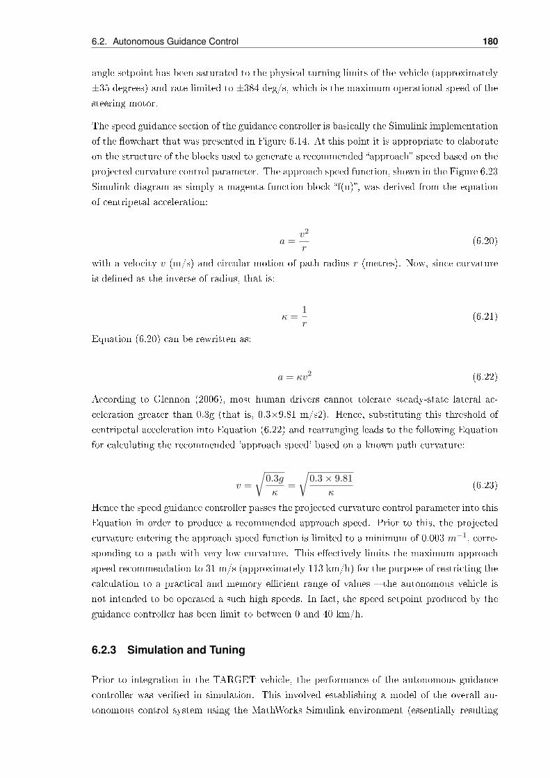
6.2. Autonomous Guidance Control 180
angle setpoint has been saturated to the physical turning limits of the vehicle (approximately
±35 degrees) and rate limited to ±384 deg/s, which is the maximum operational speed of the
steering motor.
The speed guidance section of the guidance controller is basically the Simulink implementation
of the owchart that was presented in Figure 6.14. At this point it is appropriate to elaborate
on the structure of the blocks used to generate a recommended approach speed based on the
projected curvature control parameter. The approach speed function, shown in the Figure 6.23
Simulink diagram as simply a magenta function block f(u), was derived from the equation
of centripetal acceleration:
a =v2
r(6.20)
with a velocity v (m/s) and circular motion of path radius r (metres). Now, since curvature
is dened as the inverse of radius, that is:
κ =1r
(6.21)
Equation (6.20) can be rewritten as:
a = κv2 (6.22)
According to Glennon (2006), most human drivers cannot tolerate steady-state lateral ac-
celeration greater than 0.3g (that is, 0.3×9.81 m/s2). Hence, substituting this threshold of
centripetal acceleration into Equation (6.22) and rearranging leads to the following Equation
for calculating the recommended 'approach speed' based on a known path curvature:
v =
√0.3gκ
=
√0.3× 9.81
κ(6.23)
Hence the speed guidance controller passes the projected curvature control parameter into this
Equation in order to produce a recommended approach speed. Prior to this, the projected
curvature entering the approach speed function is limited to a minimum of 0.003 m−1, corre-
sponding to a path with very low curvature. This eectively limits the maximum approach
speed recommendation to 31 m/s (approximately 113 km/h) for the purpose of restricting the
calculation to a practical and memory ecient range of values the autonomous vehicle is
not intended to be operated a such high speeds. In fact, the speed setpoint produced by the
guidance controller has been limit to between 0 and 40 km/h.
6.2.3 Simulation and Tuning
Prior to integration in the TARGET vehicle, the performance of the autonomous guidance
controller was veried in simulation. This involved establishing a model of the overall au-
tonomous control system using the MathWorks Simulink environment (essentially resulting

181 Chapter 6. Control Strategies
Figure 6.24: Autonomous control simulation model
Figure 6.25: Motion Execution Controller model
in a virtual model of the system owchart presented in Figure 6.12). The top level of the
resulting model is shown in Figure 6.24 and includes a waypoint denition block, the afore-
mentioned Parameter Calculator and Guidance Controller (refer to Section 6.2.2), a block
representing the Motion Execution Controller, and a mathematical vehicle model.
The dummy Motion Execution Controller block contains two rst-order transfer functions
as shown in Figure 6.25, one for steering and one for speed. It was estimated that it would
take approximately one second for the real Motion Execution Controller (discussed in Sec-
tion 6.3) to control the actual vehicle steering to the commanded steering angle setpoint,
and approximately four seconds to achieve the speed setpoint. The time constants of the
rst-order transfer functions were therefore tuned to replicate these delays. Their unit step
response is shown in Figure 6.26.
6.2.3.1 Mathematical Vehicle Model
A mathematical model of the relevant vehicle dynamics was derived in order to test and
tune the Autonomous Guidance Controller prior to its integration with the actual TARGET
vehicle. The development of an accurate mathematical vehicle model had also been dened
as one of the project goals. The mathematical vehicle model needed to relate the vehicle
speed and wheel angle theoretically achieved by the guidance controller (in combination with
motion execution control) to the instantaneous vehicle states of heading (θ), Easting (E), and
Northing (N) which are required as inputs to the autonomous controller. Using the variable
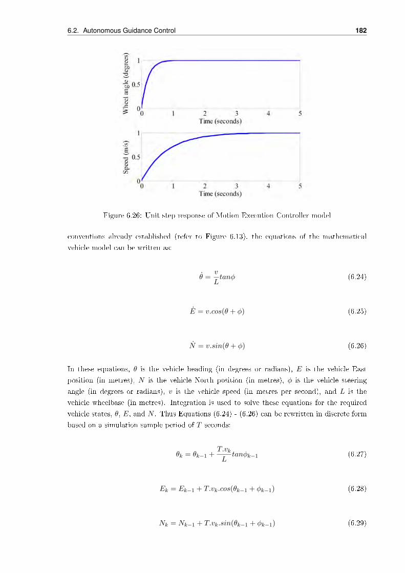
6.2. Autonomous Guidance Control 182
Figure 6.26: Unit step response of Motion Execution Controller model
conventions already established (refer to Figure 6.13), the equations of the mathematical
vehicle model can be written as:
θ =v
Ltanφ (6.24)
E = v.cos(θ + φ) (6.25)
N = v.sin(θ + φ) (6.26)
In these equations, θ is the vehicle heading (in degrees or radians), E is the vehicle East
position (in metres), N is the vehicle North position (in metres), φ is the vehicle steering
angle (in degrees or radians), v is the vehicle speed (in metres per second), and L is the
vehicle wheelbase (in metres). Integration is used to solve these equations for the required
vehicle states, θ, E, and N . Thus Equations (6.24) - (6.26) can be rewritten in discrete form
based on a simulation sample period of T seconds:
θk = θk−1 +T.vkL
tanφk−1 (6.27)
Ek = Ek−1 + T.vk.cos(θk−1 + φk−1) (6.28)
Nk = Nk−1 + T.vk.sin(θk−1 + φk−1) (6.29)
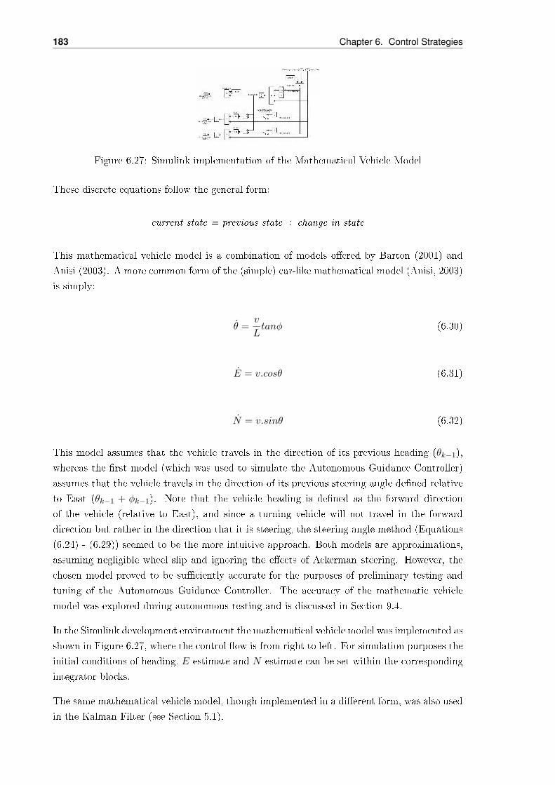
183 Chapter 6. Control Strategies
Figure 6.27: Simulink implementation of the Mathematical Vehicle Model
These discrete equations follow the general form:
current state = previous state + change in state
This mathematical vehicle model is a combination of models oered by Barton (2001) and
Anisi (2003). A more common form of the (simple) car-like mathematical model (Anisi, 2003)
is simply:
θ =v
Ltanφ (6.30)
E = v.cosθ (6.31)
N = v.sinθ (6.32)
This model assumes that the vehicle travels in the direction of its previous heading (θk−1),
whereas the rst model (which was used to simulate the Autonomous Guidance Controller)
assumes that the vehicle travels in the direction of its previous steering angle dened relative
to East (θk−1 + φk−1). Note that the vehicle heading is dened as the forward direction
of the vehicle (relative to East), and since a turning vehicle will not travel in the forward
direction but rather in the direction that it is steering, the steering angle method (Equations
(6.24) - (6.29)) seemed to be the more intuitive approach. Both models are approximations,
assuming negligible wheel slip and ignoring the eects of Ackerman steering. However, the
chosen model proved to be suciently accurate for the purposes of preliminary testing and
tuning of the Autonomous Guidance Controller. The accuracy of the mathematic vehicle
model was explored during autonomous testing and is discussed in Section 9.4.
In the Simulink development environment the mathematical vehicle model was implemented as
shown in Figure 6.27, where the control ow is from right to left. For simulation purposes the
initial conditions of heading, E estimate and N estimate can be set within the corresponding
integrator blocks.
The same mathematical vehicle model, though implemented in a dierent form, was also used
in the Kalman Filter (see Section 5.1).

6.2. Autonomous Guidance Control 184
Table 6.4: Autonomous Guidance Control Performance ComparisonCross-track error measurement (metres) TARGET Guidance Controller Barton's Guidance Controller Performance Improvement (%)
Maximum (m) < 0.03 0.6 95
Mean (m) < 0.007 0.2 97
Standard deviation (m) < 0.01 0.1 90
6.2.3.2 Simulated Performance Results
The performance of the Autonomous Guidance Control was simulated and tuned using the
Simulink model presented in Figure 6.24, which is equipped with the Mathematical Vehicle
Model detailed in the previous section (Section 6.2.3.1). The key performance measure for the
Autonomous Guidance Controller is the cross-track error, as this indicates the vehicle's lateral
deviation from the path. Aside from some minor adjustment in the Parameter Calculator,
the Autonomous Guidance Controller was essentially tuned by manually adjusting the four
control gains in the Guidance Controller block (refer to Figure 6.23).
The simulated path-tracking performance of the well-tuned Autonomous Guidance Controller
to an open and closed-circuit waypoint-dened path is presented in Figures 6.28 and 6.29. The
upper graph in these gures shows the vehicle trajectory (red) as it attempts to autonomously
follow the desired path (blue), and the corresponding time-based cross-track error measure-
ments which provides a more quantiable gauge of the autonomous path-tracking performance.
In particular note the maximum, mean and standard deviation of the cross-track error. The
cross-track error varies over time rather than settling on a single steady-state value because
of the curvature variation in the desired paths. The other two graphs in each gure indicate
the steering angle guidance setpoint and actual vehicle speed response of the autonomous
vehicle for the given path.
These were impressive results. It should be kept in mind, however, that these simulations
were made using precise estimates of the vehicle's position and heading. In reality, additional
path-tracking inaccuracy arises, through no fault of the Guidance Controller, as a result of
using estimated vehicle position and heading values. Although these vehicle state estimates
supplied by the Kalman Filter are an improvement on raw sensor information, they constitute
the primary limitation on the overall path-tracking performance achievable in eld testing.
The simulated results of the Autonomous Guidance Controller reveal a signicant perfor-
mance improvement over the virtual vehicle based path-tracking controller presented in Bar-
ton (2001). Barton's controller was simulated using a constant vehicle speed of 20 km/h, a
maximum steering angle command of 15 degrees, and a mathematical vehicle model very simi-
lar to the one adopted in this project (Barton, 2001), thereby enabling reasonable comparisons
to be made with the simulation results of the TARGET Autonomous Guidance Controller. A
performance comparison is provided in Table 6.4. The closed-circuit path corresponding to
Barton's results is shown in Figure 3.20 of the Literature Review.
The performance of the Autonomous Guidance Controller during on-the-road autonomous
operation is discussed in Section 9.4.
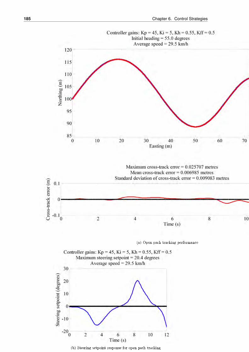
185 Chapter 6. Control Strategies
(a) Open path tracking performance
(b) Steering setpoint response for open path tracking
(c) Speed response for open path tracking
Figure 6.28: Simulated open path-tracking performance of the Autonomous Guidance Con-troller

6.2. Autonomous Guidance Control 186
(a) Closed-circuit path tracking performance
(b) Steering setpoint response for closed-circuit path tracking
(c) Speed response for closed-curcuit path tracking
Figure 6.29: Simulated closed-circuit path tracking performance of the Autonomous GuidanceController

187 Chapter 6. Control Strategies
6.3 Motion Execution Control
The Motion Execution Control System acts as the link between driving commands and the
actuators. The system has two independent inputs, but only one of these inputs are active
at any given moment, depending on whether the vehicle is in radio control or autonomous
mode. In radio control mode, the Motion Execution Control System receives commands from
a human operator via the handheld controller. In autonomous mode, commands are received
from the Autonomous Guidance Control System. Its purpose is to ensure that these commands
are implemented eectively by sending the correct signals to the actuators (steering, brake
and throttle).
The controller is split into two separate systems: steering control and speed control. The
speed control loop contains two sub-loops to control the brake and throttle independently.
Switching logic is used between the throttle and braking systems in order to control the
vehicle's speed. This is to mimic the behavior of a human driver as the accelerator and brake
are never operated simultaneously. Therefore only one of these controllers will be operational
at any given moment. This provides for smoother speed control and also prevents wear and
tear on the braking system. The Motion Execution Control System has been developed using
Matlab and Simulink and has been exported to run on the onboard computer using the
embedded xPC Target software as discussed in Section 4.2.1.
The performance and tuning of the Motion Execution Control system is discussed in Section
9.3. This discussion is carried out with reference to the project specications and goals which
is discussed in Chapter 2.
6.3.1 Steering Control
The steering control loop provides automatic control of the steering system in the vehicle.
It receives a normalised input command between -1 to 1 corresponding to full steering lock
left and full steering lock right respectively. Its output is the actual steering wheel position,
also normalised between -1 and 1. A top level block diagram of the steering control system is
shown in Figure 6.30.
As shown in Figure 6.30, there are three main parts to the control system. These are the
roll prevention saturation block in white, steering position control loop in dark grey and the
steering lock saturation in light grey. These three parts will be discussed in further detail in
the following sections. The inputs are the steering setpoint, actual speed feedback (provided
by the Kalman Filter as described in Section 5.1) and the steering angle (provided by the
steering potentiometer as described in Section 4.4.3). The output is the steering command
and this is the signal sent to the steering actuator.
The setpoint to the steering position control loop is provided after roll prevention saturation.
The output of the control loop is given to the steering lock prevention block before being sent

6.3. Motion Execution Control 188
Figure 6.30: Steering Control System
to the steering actuator. Control is achieved using a Proportional Derivative (PD) feedback
control structure. Integral control was not included as the actuator itself integrates a speed
to a position. The feedback is provided by the potentiometer which gives an indication of
actual steering wheel position.
6.3.1.1 Roll Prevention Saturation
As the vehicle will be moving and cornering at speed, situations may arise where the steering
setpoint causes the vehicle to turn too sharply and roll over, damaging the vehicle, the installed
hardware and injuring the occupants (if present). The purpose of the roll prevention subsystem
is to ensure that the van does not turn too sharply at higher speeds. This is achieved by using
the actual vehicle speed (feedback from the Kalman Filter) to limit the steering setpoint using
a dynamic saturation block. This is shown in Figure 6.31.
Figure 6.31: Roll Prevention Saturation
A small oset is included in order to prevent mathematical singularities if a vehicle speed of
0 is received. The value of the constants was found using analysis of the vehicle dynamics.
This analysis was carried out using standard metric units. However, the actual vehicle speed
is normalised between 0 and 1 (0 km/h to 40 km/h) so a scaling factor is also included in
order to convert to metric units so the correct saturation is provided. The actual analysis
follows:

189 Chapter 6. Control Strategies
Consider a motor vehicle traveling in an arc on a at road as depicted in Figure 6.32.
Figure 6.32: Roll Prevention Analysis 1
The parameters shown are dened as follows:
COG The centre of gravity of the vehicle
r The instantaneous turning radius of the vehicle's path
h The height of the centre of gravity above the road
b The vehicle's track width
G The acceleration due to gravity
n Safety factor (not shown in diagram)
The vehicle will tip over if the velocity is greater or equal to the following (Bosch, 2004):
v ≥ π
n
√br
2hms−1 (6.33)
The critical value of velocity occurs when the inequality becomes an equality. This can be
rearranged to nd:
r =2hb
(vnπ
)2m (6.34)
Now consider the vehicle moving in a small time period along a circular arc, from position 1
to position 2 as shown in Figure 6.33. Also shown in Figure 6.33 is a vector view of the two
velocity vectors V1 and V2, and the angle θ between them.

6.3. Motion Execution Control 190
Figure 6.33: Roll Prevention Analysis 2
Circular motion gives an instantaneous radius:
r =v
θ(6.35)
Now substituting this into Equation (6.34) and rearranging gives:
θ =bπ2
2hvn2(6.36)
Substituting the actual vehicle characteristics (b = 1.38 m, h = 1.90 m) and a safety factor
n = 1.2 gives the value used for the constant in the roll prevention saturation:
θ =4.978v
(6.37)
The value of the safety factor was chosen in order to allow for a safety buer in the roll
prevention subsystem without severely limiting the turning circle of the vehicle.
6.3.1.2 Steering Lock Saturation
The purpose of this subsystem is to ensure that the steering actuator does not continue to
turn when it reaches full lock left or full lock right. The actuator is is capable of producing

191 Chapter 6. Control Strategies
a large torque, so if it continues to turn at full lock, it could damage the sprockets, chain or
the steering column itself. This system is shown in Figure 6.34.
Figure 6.34: Steering Lock Saturation
This system uses the steering angle feedback (provided by the steering potentiometer) in order
to completely cut the steering command signal when the steering wheel reaches 85% of its
full lock and the controller continues to turn it towards full lock in either direction. This is
to ensure that there is a safety buer between the actual steering wheel position and full lock
at all times.
6.3.2 Speed Control
The speed control system provides automatic control of the vehicle's throttle and brake by
sending signals to the actuators. Its structure is more complex than the steering controller as
can be seen in Figure 6.35.
It has two modes of operation, open loop and closed loop. In open loop, the speed controller
receives a scaled input of -1 to 1 (full brake to full throttle). The throttle actuator is used
when the setpoint is between 0 and 1 (no throttle to full throttle). The brake actuator is used
when the setpoint is between 0 and -1 (no brake to full brake). In this mode of operation,
there is no speed control, only normalized position control for the brake and throttle. Open
loop mode is used only in remote control mode in conjunction with the handheld controller.
The darker grey blocks in Figure 6.35 shows the open loop control section.
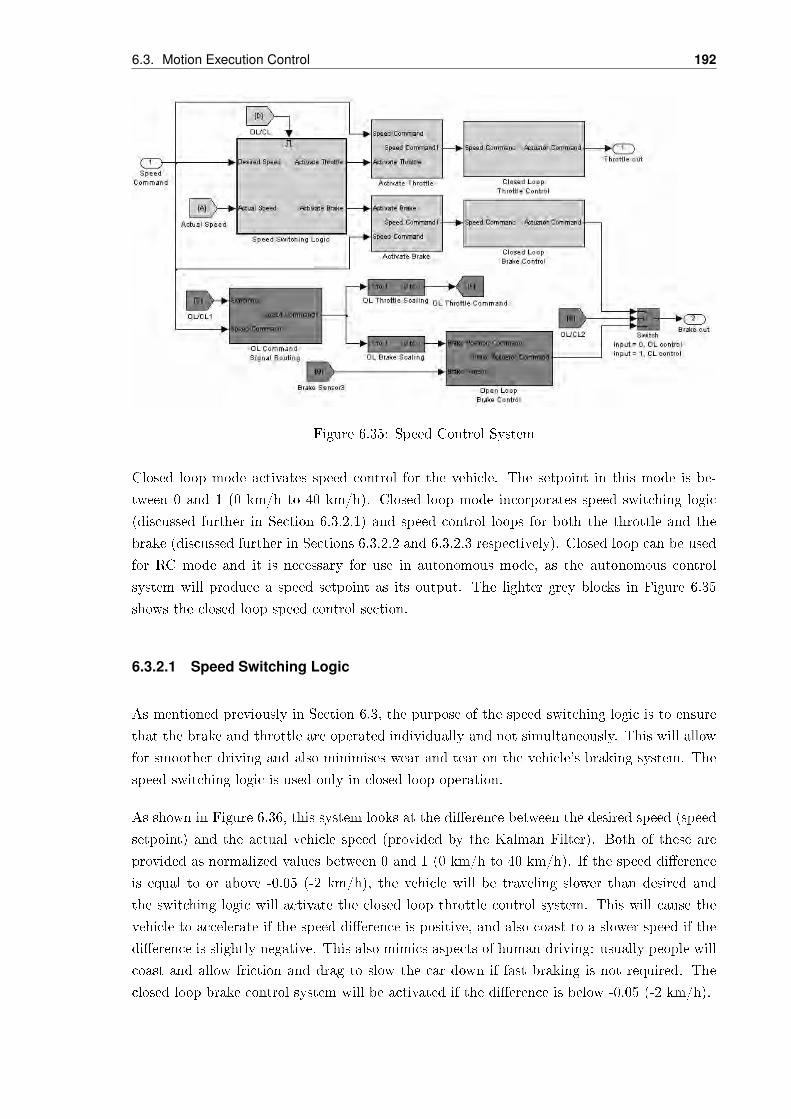
6.3. Motion Execution Control 192
Figure 6.35: Speed Control System
Closed loop mode activates speed control for the vehicle. The setpoint in this mode is be-
tween 0 and 1 (0 km/h to 40 km/h). Closed loop mode incorporates speed switching logic
(discussed further in Section 6.3.2.1) and speed control loops for both the throttle and the
brake (discussed further in Sections 6.3.2.2 and 6.3.2.3 respectively). Closed loop can be used
for RC mode and it is necessary for use in autonomous mode, as the autonomous control
system will produce a speed setpoint as its output. The lighter grey blocks in Figure 6.35
shows the closed loop speed control section.
6.3.2.1 Speed Switching Logic
As mentioned previously in Section 6.3, the purpose of the speed switching logic is to ensure
that the brake and throttle are operated individually and not simultaneously. This will allow
for smoother driving and also minimises wear and tear on the vehicle's braking system. The
speed switching logic is used only in closed loop operation.
As shown in Figure 6.36, this system looks at the dierence between the desired speed (speed
setpoint) and the actual vehicle speed (provided by the Kalman Filter). Both of these are
provided as normalized values between 0 and 1 (0 km/h to 40 km/h). If the speed dierence
is equal to or above -0.05 (-2 km/h), the vehicle will be traveling slower than desired and
the switching logic will activate the closed loop throttle control system. This will cause the
vehicle to accelerate if the speed dierence is positive, and also coast to a slower speed if the
dierence is slightly negative. This also mimics aspects of human driving: usually people will
coast and allow friction and drag to slow the car down if fast braking is not required. The
closed loop brake control system will be activated if the dierence is below -0.05 (-2 km/h).
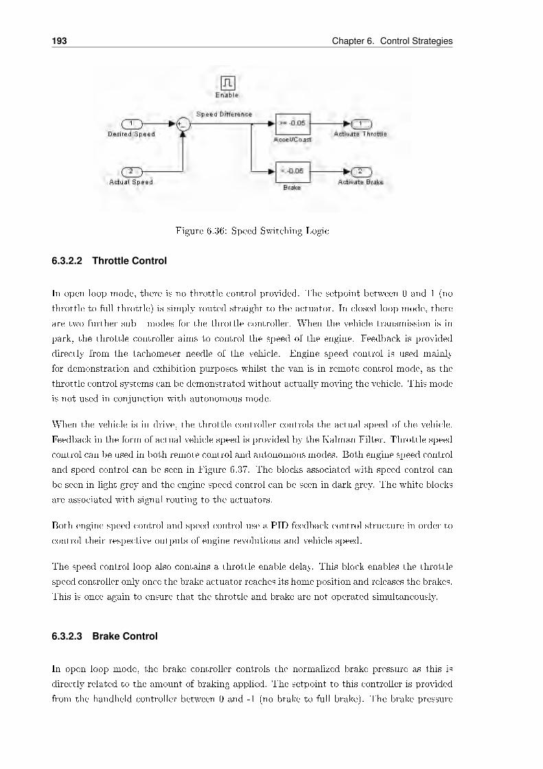
193 Chapter 6. Control Strategies
Figure 6.36: Speed Switching Logic
6.3.2.2 Throttle Control
In open loop mode, there is no throttle control provided. The setpoint between 0 and 1 (no
throttle to full throttle) is simply routed straight to the actuator. In closed loop mode, there
are two further sub - modes for the throttle controller. When the vehicle transmission is in
park, the throttle controller aims to control the speed of the engine. Feedback is provided
directly from the tachometer needle of the vehicle. Engine speed control is used mainly
for demonstration and exhibition purposes whilst the van is in remote control mode, as the
throttle control systems can be demonstrated without actually moving the vehicle. This mode
is not used in conjunction with autonomous mode.
When the vehicle is in drive, the throttle controller controls the actual speed of the vehicle.
Feedback in the form of actual vehicle speed is provided by the Kalman Filter. Throttle speed
control can be used in both remote control and autonomous modes. Both engine speed control
and speed control can be seen in Figure 6.37. The blocks associated with speed control can
be seen in light grey and the engine speed control can be seen in dark grey. The white blocks
are associated with signal routing to the actuators.
Both engine speed control and speed control use a PID feedback control structure in order to
control their respective outputs of engine revolutions and vehicle speed.
The speed control loop also contains a throttle enable delay. This block enables the throttle
speed controller only once the brake actuator reaches its home position and releases the brakes.
This is once again to ensure that the throttle and brake are not operated simultaneously.
6.3.2.3 Brake Control
In open loop mode, the brake controller controls the normalized brake pressure as this is
directly related to the amount of braking applied. The setpoint to this controller is provided
from the handheld controller between 0 and -1 (no brake to full brake). The brake pressure

6.3. Motion Execution Control 194
Figure 6.37: Closed Loop Throttle Controller
is controlled using a PID feedback control structure. The feedback is provided by the brake
pressure transducer as discussed in Section 4.6.1.3.
In closed loop mode, the brake controller controls the actual speed of the vehicle through
braking. It consists of two sub controllers, both of which use a PID feedback control structure.
The rst controller uses the actual vehicle speed feedback to generate a required braking
pressure. This braking pressure setpoint is then passed through to the same controller as for
the open loop brake control in order to send the right signal to the braking actuator. This is
illustrated in Figure 6.38.
Figure 6.38: Closed Loop Brake Controller

Chapter 7
Graphical User Interface
7.1 Software
The base station software serves as the primary interaction between user and vehicle. The
Graphical User Interface (GUI) must provide all the tools necessary to control the vehicle at
its full potential. It must also feed back the information necessary to monitor all aspects of
the vehicles motion. To do this, the software must be able to:
• Set up communication through a serial port to the TARGET vehicle (see Section 4.3.2)
• Provide the user with:
Waypoint editing functions
Vehicle status
Log les to review
• Store the list of user dened waypoints
• Generate a smooth path between the dened waypoints
• Eectively communicate the smooth path to the vehicle
Java was chosen as a suitable programming language to complete these tasks. Java has been
described as a safe and robust language that can provide high performance, cross-platform,
object oriented programs (Harold, 2000). Java:
• is widely used and so contains signicant documentation and support
• was used in similar previous projects conducted at the University of Adelaide
• was not known by any member of the group and so would provide a signicant challenge
meeting the project needs
195

7.1. Software 196
7.1.1 Software Requirements
The base station software has been designed and tested on a Windows XP computer that was
installed with the following software packages:
• Eclipse IDE Version 3.3.0 - An application that aides in software development
• Java JRE 1.6.0 & JDK 1.6.0.02- Core language for the base station software
• RXTX - A native library providing serial and parallel communication for Java
• JFreeChart - A library providing extensive support for graph, chart and dial construction
for Java
7.1.2 Design Solution
The constructed base station software has many dierent java class les and has a source code
containing 800+ lines of code. It represents many hours of research, development and testing
to make sure every aspect performs correctly. Each le has been designed and written with
a specic function, and when combined together the les form an overall program. In this
section some of the les and their functions will be explained in more detail.
Each major segment of the program has been constructed with a Manager associated with
it. The manager is responsible for all operations to do with that particular section and any
action must have permission from the manager. This system has proven to work very well
with the base station software.
Some of the main class les and managers incorporated in the base station are the Waypoint
Manager, Serial Manager, File Manager, Sound Manager, Picture Manager, MainWindow
and Vehicle States. These seven main class les work together to achieve most of the program's
major functions.
The Waypoint Manager
The waypoint manager is responsible for four separate internal lists of GPS waypoints. Each
waypoint contains specic information which is used to describe a point on the earth's surface.
Other important information contained within a waypoint includes the desired speed, if the
waypoint is selected and if the waypoint has been automatically generated. The four internal
lists are used to maintain information and ensure that data is not lost or accidentally removed.
They can be described as:
1. A list of waypoints that have been dened by the user.

197 Chapter 7. Graphical User Interface
Figure 7.1: Various path types for the same ve waypoints. The vehicle is represented as ablue dot.
2. A list of waypoints representing the smooth path displayed on the screen. These way-
points are automatically generated and also include the waypoints in list #1 above.
3. A list of waypoints that has been sent to the TARGET computer. This list is a copy of
list #2, but is updated and displayed separately.
4. A list of waypoints stored to remember the actual path of the vehicle. Ideally the path of
the vehicle will be identical to list #3, but this is not guaranteed. This list of waypoints
is also used to automatically generate a path from no-user-input waypoints.
The waypoint manager has been given the ability to add, edit and delete waypoints from all
four lists as required by the user or TARGET computer. The waypoints are either added by
the user, added from the log le or automatically generated. In the case where waypoints are
generated automatically, the waypoint manager is also responsible for the iterations required
to form a path (see Chapter 3.7). There are four separate path types that can be generated.
Paths can either be generated as open or closed loop paths and can be generated by using
either linear or cubic splines. Figure 7.1 illustrates how the waypoint manager draws these
four dierent path types between the vehicle and a collection of waypoints.
The Serial Manager
The serial manager is responsible for opening and maintaining the serial port communication
with the TARGET vehicle. All data sent to and received from the serial port is managed by

7.1. Software 198
Figure 7.2: Event sequence showing data inow, events and event recipients
the serial manager. Another main function of the serial manager is to trigger events, which
calls other objects in the program to perform an action. An example is when the position of
the vehicle changes. The change in position must be correctly displayed on the screen and
the serial manager triggers this event. The information included in the event is sucient
to identify what actions must be taken by the receiving objects. Figure 7.2 illustrates what
occurs when data is recieved on the serial port. An event is generated and passed to all objects
registered to listen for serial manager events.
Setting up a serial port connection is very simple. Controls have been interfaced between the
MainWindow and the serial manager to help during testing stages. The user has two options
relating to the serial port which is used. The speed and serial port number can easily be
changed by selecting the correct settings on the visual display.
The File Manager
The le manager is responsible for all the interactions that the program has with external
les. There are three main le types the program must interact with. These include:
• Conguration Files are used to help dene the background images. The le manager
reads and interprets the information and can pass all the required data to the picture
manager where the pictures are stored.
• Background Images are requested by the picture manager. The data is read by the le
manager and then passed to the picture manager.
• Log Files
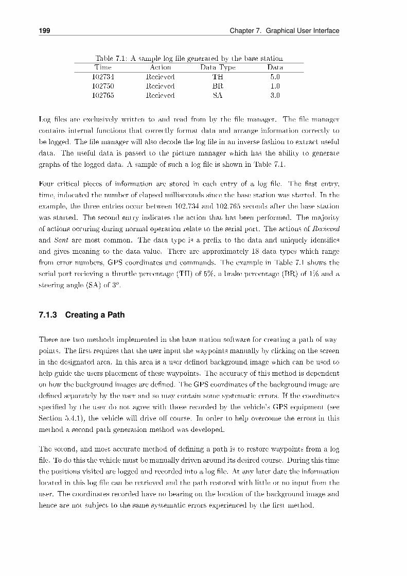
199 Chapter 7. Graphical User Interface
Table 7.1: A sample log le generated by the base stationTime Action Data Type Data
102734 Recieved TH 5.0102750 Recieved BR 1.0102765 Recieved SA 3.0
Log les are exclusively written to and read from by the le manager. The le manager
contains internal functions that correctly format data and arrange information correctly to
be logged. The le manager will also decode the log le in an inverse fashion to extract useful
data. The useful data is passed to the picture manager which has the ability to generate
graphs of the logged data. A sample of such a log le is shown in Table 7.1.
Four critical pieces of information are stored in each entry of a log le. The rst entry,
time, indocated the number of elapsed milliseconds since the base station was started. In the
example, the three entries occur between 102.734 and 102.765 seconds after the base station
was started. The second entry indicates the action that has been performed. The majority
of actions occuring during normal operation relate to the serial port. The actions of Recieved
and Sent are most common. The data type is a prex to the data and uniquely identies
and gives meaning to the data value. There are approximately 18 data types which range
from error numbers, GPS coordinates and commands. The example in Table 7.1 shows the
serial port recieving a throttle percentage (TH) of 5%, a brake percentage (BR) of 1% and a
steering angle (SA) of 3o.
7.1.3 Creating a Path
There are two methods implemented in the base station software for creating a path of way-
points. The rst requires that the user input the waypoints manually by clicking on the screen
in the designated area. In this area is a user dened background image which can be used to
help guide the users placement of these waypoints. The accuracy of this method is dependent
on how the background images are dened. The GPS coordinates of the background image are
dened separately by the user and so may contain some systematic errors. If the coordinates
specied by the user do not agree with those recorded by the vehicle's GPS equipment (see
Section 5.4.1), the vehicle will drive o course. In order to help overcome the errors in this
method a second path generation method was developed.
The second, and most accurate method of dening a path is to restore waypoints from a log
le. To do this the vehicle must be manually driven around its desired course. During this time
the positions visited are logged and recorded into a log le. At any later date the information
located in this log le can be retrieved and the path restored with little or no input from the
user. The coordinates recorded have no bearing on the location of the background image and
hence are not subject to the same systematic errors experienced by the rst method.
7.2. Hardware 200
7.1.4 Known Issues
Memory Consumption
The base station software can be asked to import and display any number of images and so
issues have risen with the memory consumption of the program. The default allocation of
memory for a Java program is 64Mb, however after loading ve images of reasonable size, an
'OutOfMemory' error was triggered and some images would not be displayed. To overcome
this, the memory allocation for the program must be increased.
Increasing the memory allocated to the Java program cannot be done from within the program
itself. The extra memory must be allocated before the program is run and nothing can be
added to this allocation once initialized. To increase the allocated memory some additional
arguments must be used. The argument '-Xmx###m' must be added, where '###' rep-
resents the number of megabytes to be allocated. It was found that an allocation of 128Mb
(or double the default allocation) was sucient to display the test images. An allocation of
512Mb has since been recommended and used. The argument can either be implemented
within Windows or included in a batch le used to initialise the base station software.
Background Image Definition
The accuracy of a background image denition is not the best it could be. Of the three
methods discussed in Section 3.8, only the rst and most basic has been implemented. The
problems and a possible solution has also been discussed in Section 7.1.3.
7.2 Hardware
The base station hardware consists of a computer, a serial modem and a power source. Because
the base station software is Java based and can be compiled for nearly all operating systems,
there is only one requirement for the computer. The computer must have at least one but
preferably two serial ports. The base station computer was initially budgeted as a Dell
desktop, but due to the large cost of such an item, it was provided 'in kind' by the university
for use throughout the project.
The selected power source is a small petrol generator. During normal operation the generator
would have to power the base station computer (including the monitor) and the serial modem.
During testing, however, the generator would also be required to power an additional computer
and monitor which must be used as the xPC host computer. The cost of a small generator
was signicantly lower than purchasing a battery and inverter. The useful running time of
the generator is also around 6 hours, which is signicantly longer than any suitable battery
could provide.

201 Chapter 7. Graphical User Interface
7.3 Final Design
The nal design of the base station software does not show many of the components described
in Section 7.1. Many of the components described in Section 7.1.2 can be seen both in Figures
7.3 and 7.4. Figure 7.3 represents a simplied ow diagram of the overall base station software.
Figure 7.4 shows a screen shot of the software package.
Figure 7.3: Simplied ow diagram of the overall base station software. Blue represents aninternal manager, orange represents the visual objects on the monitor, yellow represents datastorage and green represents external objects.

7.3. Final Design 202
Figure 7.4: Screen shot of the current base station software

Chapter 8
Safety
Safety is very important in most situations and this is especially true for this project. Because
the TARGET vehicle is a large van, all the dangers associated with a moving vehicle are
present. In addition, RC and autonomous modes introduce further risks associated with
computer based control, as there may not be a human present inside the vehicle. During its
operation, there is the potential for the TARGET vehicle to inict damage on itself, its users,
bystanders, and the surrounding environment. Because of this potential for damage, many
dierent independant systems have been developed to ensure the safety of all equipment,
people, and the surroundings. This chapter will discuss the types of emergency stops used in
the vehicle, summarise the safety systems discussed throughout the report, and also introduce
the Failure Mode and Eects Analysis and Safe Operating Procedure.
8.1 Types of Emergency Stop
Two dierent types of emergency stop are implemented on the TARGET vehicle. Each of these
correspond to dierent situations and they are mutually exclusive. The particular emergency
stop which is activated depends upon the problem encountered.
8.1.1 Failure Mode
This emergency stop is activated by the onboard computer. It can be activated by the fault
detection routine on the onboard computer, or by a user from a switch on the RC controller,
or by a user from a button on the base station computer. As discussed in Section 6.1.2, the
fault detection routine can nd 31 separate faults and any one of these faults will cause the
vehicle to enter Failure Mode. These 31 faults include the emergency stop activation signals
from both the RC controller and base station, and also a heartbeat failure from the dragon
board (which is discussed further in Section 8.1.2). Once failure mode is entered, the onboard
computer runs the emergency stop routine which:
203

8.1. Types of Emergency Stop 204
• Releases the throttle by using the throttle dump (discussed in Section 4.5.2)
• Sets the brake pressure to 75% using the brake pressure control loop (discussed in Section
6.3.2.3)
• Latches the steering wheel to its last position using the steering control loop (discussed
in Section 6.3.1)
• Activates the emergency brake system (discussed in Section ?? 8 seconds after activation
• Puts the vehicle into park using the transmission actuator (discussed in Section ??) 13
seconds after activation
• Turns o the engine once the vehicle is in park
• All warning lights on the vehicle are activated
• The corresponding fault sound is played on the base station
The throttle is set to dump so that the brakes can be applied eectively. The brakes are only
set to 75% rather than 100% in order to provide signicant braking without locking up the
wheels as the van is not tted with an anti - lock braking system. The steering is set to its
last known value to accommodate for a failure during the negotiation of a corner. In this
situation, it would be desirable to continue cornering rather than moving straight ahead. The
emergency brake system is activated after a period of time has elapsed in case the primary
braking system (as discussed in Section 4.6.1) has failed to stop the vehicle. Putting the
vehicle in park and turning the engine o ensures that the vehicle cannot move further and
is safe to approach.
Activating the warning lights on the vehicle provides a visual indication from a distance that
the TARGET has entered Failure Mode. The fault sound provides an audio indication of
Failure Mode at the base station and also allows for easy identication of the fault type
encountered. The dierent fault types are discussed in 6.1.2.
8.1.2 Dragon Stop
The Dragon Stop system has been developed in the event of a systems failure associated with
the onboard computer. In this case, the onboard computer will not be able to control the
vehicle. If this occurs, control of the steering, brake and throttle actuators is given to the
Dragon Stop system. This emergency stop mode is referred to as the Dragon Stop due to the
name of the micro - controller board used. The system was been developed in Matlab and
Simulink and has been exported to run on an MC9S12 Dragon12 micro - controller board.
A top level block diagram of this system is shown in Figure 8.1. The Dragon Stop system
monitors the onboard computer using a heartbeat signal pulse. The onboard computer also
monitors the redundant control system using a heartbeat signal pulse. This is so each of

205 Chapter 8. Safety
the systems can monitor if the other is operating correctly. If the Dragon Stop system stops
detecting the heartbeat given by the onboard computer, it will activate Dragon Stop mode.
If the onboard computer stops detecting the heartbeat given by the Dragon Stop system, it
will enter Failure Mode.
Figure 8.1: Dragon Stop System
Once Dragon Stop has been activated, three events occur:
• The throttle actuator is set to dump - this will completely release the throttle.
• The brake pressure is set to 75% of its full value using a PID controller identical to that
discussed in Section 6.3.2.3.
• The steering wheel is set to hold at its last known value using a PID controller identical
to that discussed in Section 6.3.1.
These three events occur simultaneously and are designed to bring the van to a stop quickly
and safely. The reasons for these three events are identical to those given in Section 8.1.1. It
is unlikely that the onboard computer will fail, so it was considered adequate that only the
events listed above (and not the other events listed in Section 8.1.1) are adequate for Dragon
Stop mode.
The heartbeat detection and the Dragon Stop routine has been tested and conrmed to work
in simulation. But unfortunately, this system has not been integrated completely with the rest
of the TARGET. This is due to an unforseen problem with RS232 communications and the
amplier that controls the steering and brake actuators (discussed in Section [4.8.4 STEER-
ING AND BRAKE AMPLIFIER]). The amplier only accepts 7 data bits with even
8.2. Safety Systems Summary 206
parity and this cannot be changed. The Motorola microcontroller included on the Dragon12
board supports multiple options for parity, however is limited to 8 or 9 data bits. The correct
commands are being sent by the Dragon12 board (as tested using Hyperterminal and RS232
communications) but the format between the two boards is incompatible.
Due to limitations with time, another system has not been developed and so an operator
should always be present within the vehicle in RC and autonomous modes to ensure that they
can take control if the onboard computer crashes.
8.2 Safety Systems Summary
The various safety systems have already been discussed in their respective sections throughout
this document. This section will summarise all of these previously mentioned systems and
list the appropriate sections as a reference.
8.2.1 The Van
It was important that the van chosen as the vehicle platform was roadworthy and safe to
drive as testing and transport requires the vehicle to be driven both manually by a human
and automatically in RC and autonomous modes. A cargo barrier was installed to ensure
that any equipment in the rear of the vehicle will not harm the occupants of the cabin in a
crash. The details of the vehicle selection are outlined in Section 4.1.
8.2.2 Communications
The handheld controller includes a switch to activate Fault Mode remotely, as discussed in
Section 4.3.1. This is to allow the user to manually stop the vehicle in RC mode. In addition,
a routine is included in the onboard computer program to allow for monitoring of the signal
transmitted by the handheld controller. When the RC receiver cannot detect a transmitted
signal, its output is completely static. The fault detection routine checks to see if the output
is static and activates Fault Mode if communications loss is detected. This fault detection
routine is detailed further in Section 6.1.2.3.
The RF link between the base station and the onboard computer is monitored using a heart-
beat pulse which is echoed back and forth between the two computers. If this heartbeat pulse
is not received, then the vehicle will enter Fault Mode mode as discussed in Section 6.1.1.3.
8.2.3 Actuators
The actuators and mounting were chosen with regard to ensuring safety.
207 Chapter 8. Safety
The steering motor chosen incorporates a large design factor which ensures that it can produce
more than enough torque to turn the steering wheel at all times, even in the event that power
steering is lost. To ensure the vehicle was road legal, the actuator was mounted so that it was
in compliance with requirements set by Transport SA regarding safety of the vehicle. This
was to ensure that in the event of a collision, the existing safety collapsing mechanism of the
steering column was not interfered with. This is discussed further in Section 4.4.
The throttle actuator incorporates a safety dump so that the throttle can be completely
released at any time (this is discussed in further detail in Section 4.5.2). This ensures that
the onboard computer or Dragon Stop System can release the throttle quickly at any time.
The mounting of the primary braking system discussed in Section 4.6.1 ensures that the driver
(if present) can operate the brake pedal safely and without any intereference. The actuator was
also chosen with a large design factor to ensure the brake pedal can be completely depressed.
The emergency brake system acts as a secondary braking system. It was designed to allow the
vehicle's brake pedal to be operated if electrical power is lost. The emergency brake system
is used when the vehicle enters Fault Mode as discussed in Section 8.1.1 and also if electrical
power is lost. This system is detailed in Section ??.
8.2.4 Electronics
The electronics for the TARGET vehicle have been designed with considerations made to
safety.
The existing car battery was complemented by adding a second, deep discharge battery whose
performance allows for the onboard systems to run for approximately 10 hours. A dual battery
isolatar was also installed to allow for both batteries to be charged by the alternator when
the engine is running. This ensures that there will always be enough power for the onboard
systems. This is detailed further in Section 4.8.1.
Three separate safety electronic systems were implemented as discussed in Section 4.8.2:
1. A series of relays allows power to be cut to all the actuation systems on the vehicle. This
can be operated digitally by the onboard computer system, or maually using a large red
switch located in the center console in the vehicle. This allows a driver (if present) to
regain manual control of the vehicle.
2. A proximity sensor was installed onto the brake pedal. This senses if an object (ie. the
driver's foot) is close to the pedal and also cuts power to all the actuators allowing the
driver to regain manual control of the vehicle.
3. An isolating switch was installed which cuts power to all electronics connected to the
secondary battery excluding the inverter.

8.2. Safety Systems Summary 208
In addition, many fuses have been installed (in addition to the vehicle's existing fuses) to
prevent large power surges damaging equipment inside the TARGET vehicle.
8.2.5 Autonomous Guidance Control
The Autonomous Guidance Controller contains a number of strategies to provide safe control
of the vehicle whilst in autonomous mode. A general feature of this system is that it is an
enabled subsystem of the larger onboard computer program. This means it is not running
all the time and is only activated when it is deemed safe to do so by the user.
The steering guidance controller has eective performance and consistent behaviour. This
helps create smoother steering for the vehicle whilst in autonomous mode. The output of the
steering guidance controller is also limited in range and rate to provide for smoother steering
and also decreases the chance that the vehicle will roll over. This is discussed in Section
6.2.1.1.
The speed guidance controller contains an approach speed function which checks the curvature
of a number of the upcoming path segments and suggests a safe speed. This is to maintain
a comfortable lateral acceleration of 0.3g for any occupants and also decreases the chance of
the vehicle rolling over. The speed guidance controller also contains a speed lter which slows
down and eventually stops the TARGET vehicle if it signicantly deviates from the desired
path. The speed of the vehicle is also limited to 40 km/h in autonomous mode. All of these
safety features are discussed in further detail in Section 6.2.1.2.
8.2.6 Motion Execution Control
The Motion Execution Controller also contains a number of strategies to provide for safe
control of the vehicle both in RC mode and autonomous mode.
As discussed in Section 6.3.1.1, the steering control system incorporates roll prevention. The
Autonomous Guidance Controller's steering output is range and rate limited (as discussed in
Section 6.2.1.1) which helps to prevent roll. However, this does not mean that the vehicle will
not be able to roll over if turning too sharply at high speeds. The roll prevention system in
the Motion Execution Controller ensures that the steering becomes limited as the vehicle's
speed increases and so prevents the vehicle from rolling over. This system operates in both
autonomous and RC modes.
The steering control system also incorporates a subsystem which prevents the actuator from
turning when the steering wheel is close to its full lock to the left or right as discussed in
Section 6.3.1.2. Since the motor is powerful and can produce a large torque, this subsystem
prevents the motor from damaging the mounting brackets, sprockets, chain or the steering
column itself.
209 Chapter 8. Safety
A speed switching logic is included in the speed controller as discussed in Section 6.3.2.1. This
ensures that the brake and throttle are operated individually and not simultaneously, which
provides for smoother and safer speed control of the vehicle. This also means less wear and
tear on the braking system of the vehicle.
8.3 Failure Modes and Effect Analysis
All designs which have been implemented have been made with safety as the rst priority.
This is well illustrated in the Failure Modes and Eects Analysis (FMEA), which can be
found in Appendix D. The FMEA documents the safety issues for all sections of the project
(Communications, Actuators, State Measurement and Estimation, Autonomous Guidance
Control, Motion Execution Control and GUI). This document is a standard procedure for large
projects and identies the things which can go wrong, how this can eect the performance
of the project and how these can be prevented. By identifying these issues, the design of the
various sections of the project have been improved to be safer. The FMEA includes:
• Failure Mode - this identies ways in which each component can fail
• Eect of Failure - outlines the eect the failure will have on the TARGET vehicle
• Severity Rating - the degree of severity on a scale from 1 to 10 (minor to catastrophic)
for each failure
• Potential Cause of Failure - self explanatory
• Occurence Rating - the likelihood of the failure occuring on a scale from 1 to 5 (practi-
cally never to very likely)
• Possible Means of Detection - self explanatory
• Detection Rating - the degree of diculty in detecting the failure from 1 to 10 (easily
detectable to not detectable)
• Preventative Action - self explanatory
• Action to be Taken in Case of Failure - self explanatory
8.4 Safe Operating Procedure
A document outlining the required safe operating procedure of the TARGET vehicle has been
generated to ensure the safety of the project members and general public. The document
covers the safety procedures and requirements that must be met during the testing process.
The document is separated into the following sections:

8.4. Safe Operating Procedure 210
• The procedure that must be carried out before manual transportation of the vehicle
• The start up procedure that must be carried out before testing
• General safety practices
• The procedure that must be carried out in the event of an emergency
The safe operating procedure document can be found in Appendix E.
Chapter 9
Final Testing and Analysis
9.1 Normal Operation
9.2 Actuator and Actuator Control
This section asseses the goals of the actuatiors and actuator control section of the TAR-
GET project. The goals set cover the areas of; selection of suitable hardware, installation of
hardware, design of the local control loops and the safety of the actuation systems.
9.2.1 Selection of suitable hardware
It is desireable to have actuators that possess sucient torque and force to actuate the steering,
throttle, transmission and brake of the vehicle. These actuators must also move at a rate quick
enough to mimic a human driver.
The actuators used in the TARGET vehicle successfully provided adequate force (brake,
transmission and throttle) and torque (steering) to actuate the vehicle driving controls. The
selected steering motor possesed sucient torque to actuate the steering and this was demon-
strated in testing. The motor was also capable of providing enough torque to dry steer the
vehicle. The speed at which the steering column could be turned was greater than the required
speed of 1 rev/s (see Section 4.4.1).
The selected actuators for brake and transmission possed sucient force to operate the vehicle
brake pedal and transmission lever respectively. On the other hand, the actuators are not easy
to be back driven. The issue was not considered as a major concern since regaining manual
control for vehicle brake and transmission can be perform instantaneously via removing the
R-pin connected to the actuators.
The vacuum actuator used to actuate the throttle of the vehicle was able to provide adequate
force to move the throttle valve, and also moved it at a suitable rate. Using the vacuum
actuator the vehicle achieved the required speed of 40 km/h during testing (see Chapter 2).
211

9.3. Radio Controlled Motion 212
9.2.2 Installation of steering, throttle, brake, gear stick and ignition actuators
The locations of the actuators should be chosen so as not to interfere with the normal human-
driven operation of the vehicle that is, the vehicle should be capable of being safely and legally
driven by project team members when not being driven through remote or autonomous means.
Where practically possible, functionally appropriate and without contravening the previous
statement, actuators should generally be placed in locations that are readily accessible. Wiring
should be enclosed and arranged in a neat and tidy manner.
The mounting positions of the actuation systems did not interfere with the normal operation
of the vehicle. Furthermore, the mounting arrangement for the motor and actuator was in
compliance with requirements set by Transport SA regarding safety of the vehicle (discussed
in Section 4.4.2). The actuators are also mounted so that they are accessible for maintenance
and inspection purposes. Wiring to the actuators is enclosed in a neat and tidy manner.
9.2.3 Design of local control loops for each actuator
Control loops for the actuators should maintain, as close as possible, the parameters provided
to it by either the Phase One or Phase Two control loops.
The control loops generated were incorperated into the Motion Execution Controller. Desire-
ble results were achieved and the performance is discussed in Section 9.3.
9.2.4 Safety
A reliable, fail safe mechanism for manually overriding the actuators will be developed to
enable a person in the driving seat to either immediately and easily stop or regain manual
control of the vehicle at any time.
A series of relays were installed into the TARGET vehicle to ensure that the actuators could
be disabled at anytime (see Section 4.8.2). When the actuators have been disabled a human
driver is able to regain manual control of the vehicle. Operation of the brake and throttle are
unaected when power is cut to the actuators. To steer the vehicle the steering motor must
be backdriven, which can be done with ease. To use the transmission, the transmission lever
and actuator must be disconnected by removing the R-pin holding them together.
9.3 Radio Controlled Motion
One of the project goals for the TARGET project is:

213 Chapter 9. Final Testing and Analysis
Achieve successful remote controlled operation of the target vehicle
All of the predescribed safety mechanisms will be tested and their eective and consistent
dependability ensured before operating the vehicle by remote or autonomous means. The per-
formance of the remote control vehicle operation will be assessed in a number of trials. The
underlying Motion Execution Control system will also rst be tested in simulation before being
implemented in practice. Important criteria will include operability, responsiveness, stability
and reliability, and command following. (see Section 2.2)
The safety systems included on the TARGET vehicle (apart from the Dragon Stop system)
have all been implemented and tested. These are outlined in further detail in Chapter 8. The
Motion Execution Controller was tested in simulation using Simulink to conrm the control
strategy, and also in the lab whilst the vehicle was jacked up on stands. This was to ensure
that the behaviour of the control system was as expected, before the vehicle was taken for
eld testing. Radio controlled motion of the TARGET vehicle has been successfully achieved
in the eld using both open loop and closed loop speed modes (discussed further in Section
6.3.2).
The Motion Execution Controller is responsible for radio controlled motion so this section
will discuss and analyse the results of the Motion Execution Control system as implemented.
The analysis includes tuning and performance of the control systems (steering and speed
controllers) with reference to the project goals and specications (as discussed in Section 2.1.5.
The Motion Execution Controller is associated with implementing the commands outputted
by the Autonomous Guidance Controller in autonomous mode along with RC mode. However,
the performance of the Motion Execution Control system is identical in both autonomous and
RC operation, as the only dierence is the source of the inputs. Hence, this section will only
discuss the performance of the Motion Execution Control System whereas Section 9.4 will
discuss the performance of the Autonomous Guidance Controller.
9.3.1 Vehicle Steering and Speed Control
The desired vehicle heading and speed are to be transmitted to the onboard processor from the
handheld, human operated radio control via the one way communication link as inputs to the
Motion Execution Control system. When operating in autonomous mode, the desired vehicle
heading and speed will be generated by the Autonomous Guidance Control system and passed
on to the Motion Execution Controller. Closed loop feedback of the 'actual' vehicle steering
and speed will be provided by a Kalman Filter / estimator via a fusion of measurements from
the GPS, IMU, and other available vehicle sensors. The Motion Execution Control system
will then regulate output commands to the throttle, steering and brake actuators and ensure
that the vehicle responsively tracks the desired steering and speed. (see Section 2.1.5)
The Motion Execution Controller successfully achieves control of the vehicle's steering and
speed by sending signals to the actuators. It is able to receive steering and speed inputs

9.3. Radio Controlled Motion 214
Figure 9.1: Steering step response (TBD)
Table 9.1: Steering controller step response characteristicsCharacteristic Value
Overshoot ?
Rise Time ?
Settling Time ?
Final Value ?
from both the handheld controller in RC mode and the Autonomous Guidance Controller in
autonomous mode and implement these commands onto the vehicle. The local control loops
for the actuators were originally included under the Actuator and Actuator Control subgroup
but have been developed within the Motion Execution Controller and are discussed in Sections
9.3.2 and 9.3.3.
9.3.2 Steering Controller
As discussed in Section 6.3.1, the structure of the steering controller consists of a PD controller
in a closed loop with feedback provided by the steering potentiometer. This PD controller
was tuned manually on the y using a trial and error method. Tuning methods such as the
Zeigler - Nichols method were initially considered over trial and error. However this would
have taken as much time or longer because the calculated controller gains would most likely
require further tweaking using trial and error. The acceptable gains were found to be:
Proportional 5
Derivative 0.1
These nal gains were chosen based on visual monitoring of the rise time for a setpoint as
compared with a human user operating the wheel. The rise times observed in the steering
controller were low, faster than a human could operate the wheel. Very little overshoot was
observed and this is shown in Figure 9.1.
Listed in Table 9.1 are the performance characteristics for the steering controller. These values
were found from the step response of the system as shown in Figure 9.1.
[DISCUSSION OF PERFORMANCE]
9.3.3 Speed Controller
Discussion and analysis of the performance and tuning of the speed controller must be split
into two parts: open loop mode and closed loop mode. The details of these two modes are
discussed further in Section 6.3.2.
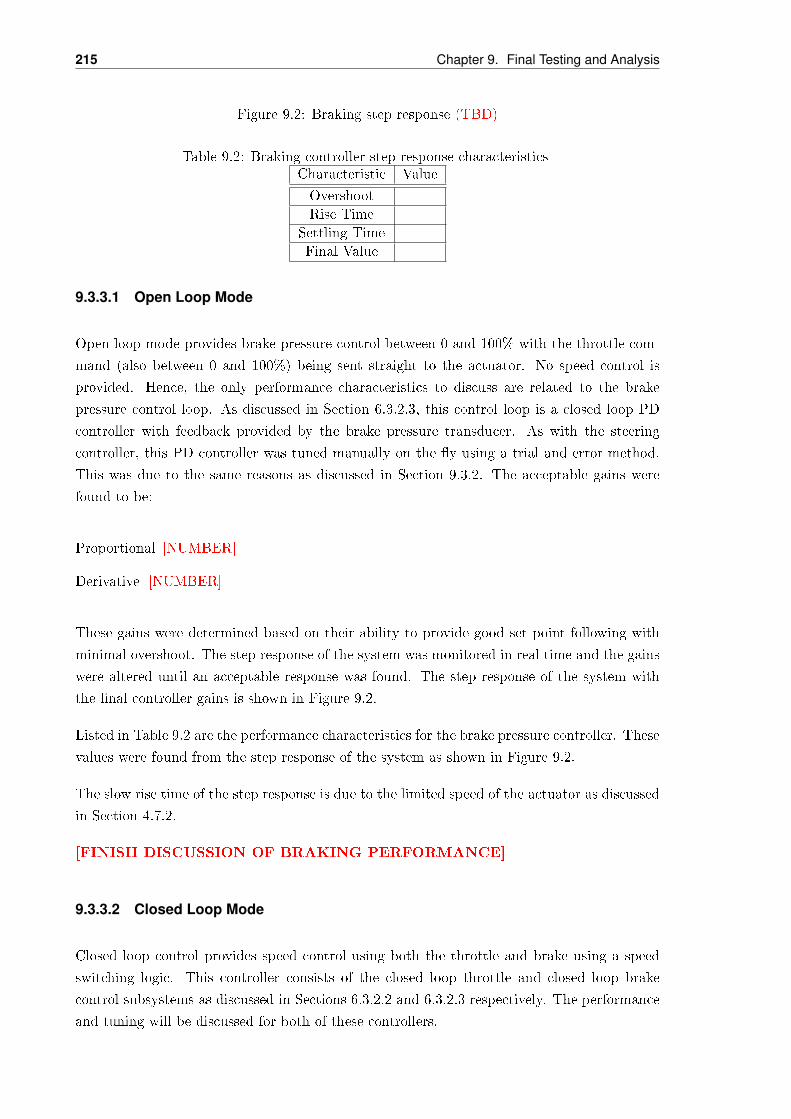
215 Chapter 9. Final Testing and Analysis
Figure 9.2: Braking step response (TBD)
Table 9.2: Braking controller step response characteristicsCharacteristic Value
Overshoot
Rise Time
Settling Time
Final Value
9.3.3.1 Open Loop Mode
Open loop mode provides brake pressure control between 0 and 100% with the throttle com-
mand (also between 0 and 100%) being sent straight to the actuator. No speed control is
provided. Hence, the only performance characteristics to discuss are related to the brake
pressure control loop. As discussed in Section 6.3.2.3, this control loop is a closed loop PD
controller with feedback provided by the brake pressure transducer. As with the steering
controller, this PD controller was tuned manually on the y using a trial and error method.
This was due to the same reasons as discussed in Section 9.3.2. The acceptable gains were
found to be:
Proportional [NUMBER]
Derivative [NUMBER]
These gains were determined based on their ability to provide good set point following with
minimal overshoot. The step response of the system was monitored in real time and the gains
were altered until an acceptable response was found. The step response of the system with
the nal controller gains is shown in Figure 9.2.
Listed in Table 9.2 are the performance characteristics for the brake pressure controller. These
values were found from the step response of the system as shown in Figure 9.2.
The slow rise time of the step response is due to the limited speed of the actuator as discussed
in Section 4.7.2.
[FINISH DISCUSSION OF BRAKING PERFORMANCE]
9.3.3.2 Closed Loop Mode
Closed loop control provides speed control using both the throttle and brake using a speed
switching logic. This controller consists of the closed loop throttle and closed loop brake
control subsystems as discussed in Sections 6.3.2.2 and 6.3.2.3 respectively. The performance
and tuning will be discussed for both of these controllers.

9.3. Radio Controlled Motion 216
The closed loop throttle controller consists of a PID controller which uses vehicle speed (pro-
vided by the Kalman lter) as its feedback.
[TALK ABOUT TUNING]
[TALK ABOUT BOTH SPEED AND ENGINE SPEED CONTROL]
[TALK ABOUT PERFORMANCE]
As discussed in Section 6.3.2.3, the closed loop speed controller uses two control loops: one to
generate a required braking pressure using actual vehicle speed as its feedback, and the braking
pressure control loop. The braking pressure control loop is identical to that used for open
loop mode and its performance and tuning are already discussed in Section 9.3.3.1. Hence,
this section will only discuss the performance and tuning of the controller that generates the
braking pressure command.
[TALK ABOUT TUNING AND PERFORMANCE]
9.3.4 Gearbox and Ignition Control
The Motion Execution Control system should also produce and handle control commands to the
vehicle ignition and gearbox, though local control loops embedded in the gearbox and ignition
actuator systems should be used to implement the actual automatic operation of these devices.
(Taken from Section 2.1.5)
Successful computer control of the gearbox and ignition has been developed. The transmission
control system is discussed further in Section [4.7 TRANSMISSION ACTUATION] and
the ignition control system is discussed further in Section [4.8.6 IGNITION BOARD].
Both of these systems have been tested and conrmed working. However, at the time of
writing, there were still some issues with both systems.
The mounting for the linear actuator used to control the transmission lever has been damaged
due to a mechanical problem with the transmission lever itself. Due to time constraints, this
system has not been re-implemented with the rest of the vehicle.
The computer controlled ignition system still works without problems. However, the problem
lies in the starter motor of the van itself. It only works intermittently, even whilst operated
by a user with the key for manual ignition. The starter motor needs to be replaced, but due
to time constraints, this has not yet been carried out at the time of writing.
9.3.5 Safe Operation
The controller must include appropriate safety logic to ensure safe operation of the vehicle,
though the vehicle should only be operated in an environment where the hazards posed to human
217 Chapter 9. Final Testing and Analysis
safety are minimal. The safety logic should include the ability to reliably override autonomous
control with radio / remote control at any time, an emergency stop mechanism, logic to halt
the vehicle during a loss of radio communications, and a roll prevention scheme. It is also
desirable for audio and visual warnings to be activated upon critical systems failure. (Taken
from Section 2.1.5)
The safe operation of the Motion Execution Controller and the rest of the TARGET's systems
has been tested and conrmed. Autonomous and RC mode can be overridden by a user inside
the vehicle in two ways. The rst method is the red switch on the centre console which
can be operated to kill power to all actuators (as discussed in Section [4.8.2 SAFETY
ELECTRONICS]). The second method involves the user simply placing their foot over the
capacitive sensor installed on the brake pedal. This has the same eect of killing power to all
actuators as discussed in [4.8.2 SAFETY ELECTRONICS].
An emergency stop system has been developed and implemented onto the TARGET vehicle.
The emergency stop system brings the vehicle to a halt quickly and safely, activates the
warning lights as a visual warning and also activates an audio warning on the base station.
This system has been tested and veried numerous times and is discussed further in Section
8.1.1.
A roll prevention scheme has been developed and included in the steering controller. This
system limits the amount of steering left or right as the vehicle's speed increases - hence,
ensuring that the van cannot turn too sharply whilst travelling at high speeds. The roll
prevention scheme is discussed in detail in Section 6.3.1.1. This system has been tested in the
lab and has been shown to limit the steering of the vehicle as its speed increases. However,
this has not been tested in the eld. This is because in order for this system to be tested
accurately, the vehicle must be purposely put in situations where it will roll over and this was
deemed to be too dangerous.
Further discussion of all safety systems incorporated in the TARGET vehicle can be found in
Chapter 8.
9.3.6 Selection, Installation and Maintenance of the Vehicle’s Onboard Pro-cessor
The project goal associated with the onboard processor is:
Select a suitable onboard vehicle processor
The suitability of the chosen onboard vehicle processor will be evaluated against the criteria
described in Section 9.3.6 of the Project Specication. (Taken from Section 2.2)
This goal has been achieved in accordance with the specications listed in Section 2.1.5.

9.4. Autonomous Motion 218
The vehicle's onboard processor will interface with many of the vehicle systems. It will however
be under the most load while processing the engagement of vehicle control, state estimation,
and communication. The onboard processor platform should have sucient memory and ops
(oating point operations per second) to handle these tasks, and should be equipped with enough
peripherals and I/O ports to allow the seamless integration and interconnection of the necessary
devices. The processor platform should be able to operate under the vibration, temperature, and
other environmental conditions inside the vehicle. It should therefore be enclosed in a suitable
housing and securely mounted in a protected location within the vehicle. For the purposes of
systems integration, servicing, and maintenance, it is also desirable for the processor platform
to have a modular design and be easily accessible. (Taken from Section 2.1.5)
The onboard processor chosen was a Pentium 4 desktop PC. The computer has a 2.8 GHz
Pentium 4 processor and provides I/O expandability with ve PCI slots as discussed in Section
[4.2.2.1 COMPUTER]. This computer has been running the entire onboard computer
program successfully in the lab and also in the eld. It includes all neccessary inputs and
outputs required as discussed in Section [6.1.1 I/O SIGNALS]. It has been mounted in the
rack inside the vehicle using an easily removable bracket and foam to ensure that it is isolated
from vibrations.
9.4 Autonomous Motion
9.5 Kalman Filter
9.5.1 Evaluation of the Accuracy of the System Model
The accuracy of the system model must be known to a high degree of condence for two main
reasons. Firstly, the vehicle may be required to be run without certain sensor corrections for a
period of time (for example in the event of GPS dropout). If this is the case then the duration
for which the state estimates remain accurate must be known and towards the end of this time
period the emergency stop procedure must be engaged. The second reason for evaluating the
accuracy of the system model is to determine the level of process noise which exists in each
of the states. These gures will be used when deriving the process noise covariance matrix
Q, which is the focus of Section 5.3.3.
To determine the accuracy of the system model, the model is to run whilst the vehicle is in
motion and the states of the model are logged to the TARGET computer. The true value of
each state which is logged must also be logged simultaneously so that a comparison may be
made between the model and the real thing. Clearly, if it where possible to determine these
true values to high accuracy then there would be little need for a system model in the rst
place. However, by carefully determining the path to be driven and by ensuring that the speed
is maintained constant for a known time period the true vehicle states may be determined at
least for the test case in question.
219 Chapter 9. Final Testing and Analysis
9.6 Phase One Communication
9.6.1 Selection of a Suitable Communication System
The Phase One activity is concerned with establishing a 'drive-by-wire' system to provide the
capacity to manoeuvre the target vehicle using a human-operated remote-control. This task will
require a hand-operated, short range, multichannel radio control (RC) transmitter to translate
remote human inputs of vehicle control commands (heading and speed) to a corresponding
onboard receiver over a one-way radio frequency (RF) communication system. PWM decoders
will be used to enable the onboard processor (necessary for control) to read the incoming com-
mands.
The chosen handheld remote-control was the JR X2720 that provided seven frequency chan-
nels. As explained in subsection 4.3.1, these frequency channels were successfully used to
control speed, steering, ignition and emergency stop activation during the testing stages. The
vehicle transmission was initially to be controlled by one of the frequency channels on the
handheld remote-control however due to limitations of the transmitted radio channels, the
control of transmission was moved to the base station's software. A range of approximately
1.2 kilometres was obtained when the receiver's antenna was placed in the open.
9.7 Phase Two Communication
9.7.1 Selection of a Suitable Communication System
The Phase Two communication system will support two-way communication between the ve-
hicle's onboard processor and the remote base station computer allowing waypoint position
commands to be sent to the vehicle and vehicle status information to be received by the remote
base station for visual display and monitoring. High speed data transfers over an approximate
range of ten kilometres and at an adequate bandwidth would be desirable for this purpose.
Two-way communication between the TARGET vehicle and the base station was successfully
achieved using the two RFI-9256 radio modems. The RFI-9256 radio modems operated with
maximum high-speed data transfers of 115.2 kbps at the modem-to-computer interface as well
as 'over-the-air'. During testing the radio diagnostic and statistics were recorded and shown
in Table 9.3. It can be concluded that the modems performed well because there were no bad
data packets or lost data packets during data transmission. A worst-case-scenario range test
was conducted in Adelaide City and yielded approximately 1.5 km.
9.8 GUI
In the initial project contract there were four separate and specic goals set out by the group.
These goals ranged from establishing communication with the vehicle processor to displaying
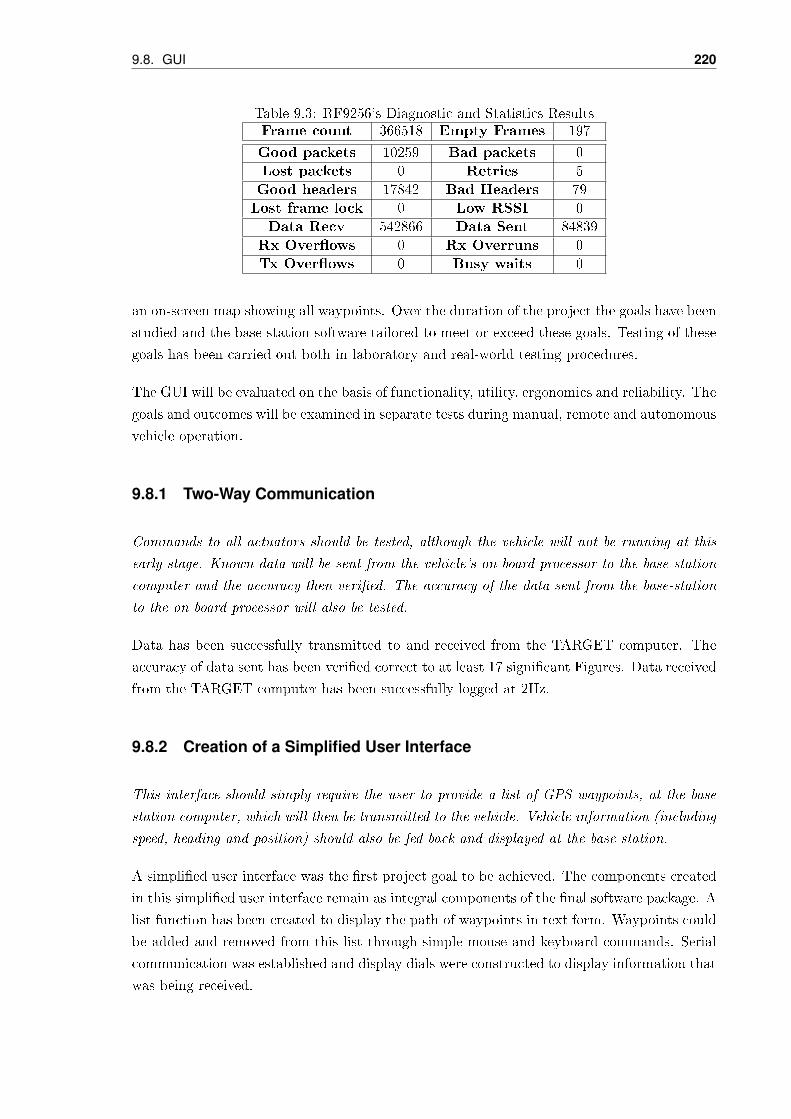
9.8. GUI 220
Table 9.3: RF9256's Diagnostic and Statistics ResultsFrame count 366518 Empty Frames 197
Good packets 10259 Bad packets 0
Lost packets 0 Retries 5
Good headers 17842 Bad Headers 79
Lost frame lock 0 Low RSSI 0
Data Recv 542866 Data Sent 84839
Rx Overows 0 Rx Overruns 0
Tx Overows 0 Busy waits 0
an on-screen map showing all waypoints. Over the duration of the project the goals have been
studied and the base station software tailored to meet or exceed these goals. Testing of these
goals has been carried out both in laboratory and real-world testing procedures.
The GUI will be evaluated on the basis of functionality, utility, ergonomics and reliability. The
goals and outcomes will be examined in separate tests during manual, remote and autonomous
vehicle operation.
9.8.1 Two-Way Communication
Commands to all actuators should be tested, although the vehicle will not be running at this
early stage. Known data will be sent from the vehicle's on board processor to the base-station
computer and the accuracy then veried. The accuracy of the data sent from the base-station
to the on board processor will also be tested.
Data has been successfully transmitted to and received from the TARGET computer. The
accuracy of data sent has been veried correct to at least 17 signicant Figures. Data received
from the TARGET computer has been successfully logged at 2Hz.
9.8.2 Creation of a Simplified User Interface
This interface should simply require the user to provide a list of GPS waypoints, at the base
station computer, which will then be transmitted to the vehicle. Vehicle information (including
speed, heading and position) should also be fed back and displayed at the base station.
A simplied user interface was the rst project goal to be achieved. The components created
in this simplied user interface remain as integral components of the nal software package. A
list function has been created to display the path of waypoints in text form. Waypoints could
be added and removed from this list through simple mouse and keyboard commands. Serial
communication was established and display dials were constructed to display information that
was being received.

221 Chapter 9. Final Testing and Analysis
9.8.3 Upgrade to a Graphical User Interface
The GUI should consist of a graphical representation of the path to be taken by the vehicle (i.e.
a map displaying all waypoints). The position of the vehicle on this map should be displayed at
the highest attainable refresh rate (depending on the hardware available) using the information
relayed back from the vehicle. The remaining vehicle states should be displayed on the GUI.
The simplied user interface was extended to include a dynamic map overlay of the vehicle and
its surroundings. Functions were added to facilitate adding, editing and deleting waypoints
from the map area. Additional features were also added to enhance the reliability an overall
functionality of the package.

9.8. GUI 222
Chapter 10
Conclusion
10.1 Achievements to Date
1. Select a suitable vehicle platform
2. Select a suitable onboard vehicle processor
3. Establish an eective automated system of actuating the vehicle driving controls without
interfering with the normal human-driven operation of the vehicle
4. Establish an eective short range one-way RF communication link between a handheld
radio control transmitter and the vehicle's onboard processor
5. Establish an eective two-way RF communication link between the remote base station
computer and the vehicle's onboard processor
6. Derive an accurate mathematical model of the relevant vehicle dynamics
7. Enable the eective fusion of all available sensor measurements into a single, more
accurate set of 'actual' vehicle states using a Kalman lter / state estimator
8. Achieve successful remote controlled operation of the target vehicle
9. Provide a graphical user interface (GUI) for the visual display and monitoring of ve-
hicle status at a portable remote base station, and allow the commanding of position
waypoints both 'on-the-y' and as a pre-programmed batch
10. Achieve successful autonomous control of the target vehicle
11. Enable intelligent and safe switching between normal human driving, remote control
and autonomous modes of operation
223

10.2. Future Work 224
10.2 Future Work
At the time of writing this document there are still many areas of the project still to be
completed. There are also many dierent areas in which the project could have been improved
if the project was undertaken again. This section aims to reect back on things that could
have changed and also look forward to future development and improvements.
10.2.1 Project Revisions
The project revisions are those that would be changed if the project was undertaken again.
10.2.1.1 xPC Embedded Computers
something about needing two one for sounds and another for control
OR something about purchasing dierent hardware to improve the sound playing performance
of the van
10.2.1.2 Pressure Transducer
use a system that does not have such unpredictable results
10.2.2 Future Development
The future development of the TARGET vehicle could involve many dierent ideas and dici-
plines. Initially, any future work undertaken on the vehicle should focus on any unaccom-
plished extension goals from the current project (see Section 2). Many dierent additions,
such as a remote camera, would be an invaluable system to be included in any future project
work.
need something to put into here

References
Single/Dual Axis Accelerometer, pages 012. Analogue Devices Inc., 0 edition, 2004a.
Single Chip Yaw Rate Gyro with Signal Conditioning, pages 012. Analogue Devices Inc., b
edition, 2004b.
David A. Anisi. Optimal motion control of a ground vehicle. Technical report, FOI Swedish
Defence Research Agency, Stockholm, jul 2003.
A. Atreya, A. Saxe, B. Collins, B. Cattle, and G. Franken. Prospect Eleven, DARPA Grand
Challenge 2005 Technical Paper, 2005.
Auscruise By Autron. Cruise Control Installation Manual, 2007.
R. Bartels, J. Beatty, and B. Barsky. An introduction to splines for use in computer graphics
and geometric modelling. 1987.
Matthew J. Barton. Controller development and implementation for path planning and fol-
lowing in an autonomous urban vehicle. Master's thesis, School of Aerospace, Mechanical
and Mechatronic Engineering, The University of Sydney, nov 2001. URL http://www.
acfr.usyd.edu.au/projects/research/ute/publication/M.%20Barton%20thesis.pdf.
D. Bevly, J. Gerdes, and B. Parkinson. A new yaw dynamic model for improved high speed
control of a farm tractor. Journal of Dynamic Systems, Measurement, and Control, 124:
659667, 2002.
Bison Gear & Engineering Corp. 2007. URL www.bisongear.com.
J. Brogdon, R. Dunlap, P. Dyson, A. Martin de Nicolas, J. Martin de Nicolas, Juan Martin
de Nicolas, D. McCauley, D. Miner, J. O'Quin, S. Polkowski, and J. Roever. Austin robot
technology, inc. darpa grand challenge 2005. Technical report, 2005.
L. Caravita, A. Tsourdos, N. Aouf, B. White, and P. Silson. Control strategies applied
to waypoint navigation and obstacle avoidance guidance. Technical report, Department
of Aerospace, Power & Sensors, Craneld University (Defence College of Management
225

References 226
UK Technology)., 2007. URL http://www.avia-it.com/act/militaravia/eventi_ami/
Militaravia_ami_agg_febb_07/2_CaravitaL_PaperACODS2007.pdf.
C. Carlson. Estimation with Applications for Automobile Dead Reckoning and Control. PhD
thesis, Department of Mechanical Engineering, Stanford University, apr 2004.
F. Caron, E. Duos, D. Pomorski, and P. Vanheeghe. Gps/imu data fusion using multisensor
kalman ltering: Introduction of contextual aspects. Information Fusion, 7:221230, sep
2006.
A. Castaño, A. Ollero, B. Vinagre, and Y. Chen. Synthesis of a spatial lookahead path
tracking controller. In 16th IFAC World Congress. IFAC, Praga, Czech Republic, 2004.
P. Coelho and U. Nunes. Path-following control of mobile robots in presence of uncertainties.
IEEE Transaction on Automatic Control, 21:2, 2003.
David C. Conner. Sensor fusion, navigation, and control of autonomous vehicles. Master's
thesis, Mechanical Engineering, Virginia Polytechnic Institute and State University, 2000.
L. Cordesses, C. Cariou, and M. Berducat. Combine harvester control using real time kine-
matic gps. Precision Agriculture, 2:147161, 2000.
J. Deak, R. Koch, G. Guthmiller, and R. Fontana. Dynamic calculation of the responsivity
of monodomain uxgate magnetometers. IEEE Transactions on Magnetics, jul 2000.
M. Egerstedt, X. Hu, and A. Stotsky. Control of mobile platforms using a virtual vehicle
approach. IEEE Transaction on Automatic Control, 46:11, 2001.
G. Elkaim, J. Connors, and J. Nagle. The overbot: an o-road autonomous ground vehicle
testbed. Technical report, University of California, Redwood City, 2006.
G. Fraichard. Fuzzy control to drive car-like vehicles. Robotics and Autonomous Systems, 24:
122, 2001.
John C. Glennon. Calculating critical speed: A motor-vehicle crash reconstruction method
fraught with error. Technical report, John C. Glennon, Chartered, 6917 West 76th Street,
Overland Park, KS 66204, aug 2006. URL http://www.johncglennon.com/papers.cfm?
PaperID=42.
S. Golconda. Steering control of a skid-steered autonomous ground vehicle at varying speed.
Technical report, The Center for Advanced Computer Studies, University of Louisiana,
Lafayette, 2005.
E. Harold. The Java Developer's Resource, 2000. URL www.cafeaulait.org/books/jdr/
chapters/01.html. accessed 15th April 2007.
D. Harper, K. Hua, H. Foroosh, Q. Leonessa, D. Harper, R. Pillat, D. Norvell, S. Santiago,
T. Collins, G. Stein, S. Stickler, G. Decker, R. Andres, Y. Shen, H. Chen, and F. Xie.
Technical paper darpa grand challenge 2005 team university of california. Technical report,
Team University of California, 2006.
227 References
John B. Herrington. Uniform Framework for GPS/IMU Integration using Kalman Filter-
ing. PhD thesis, Department of Aeronautics and Astronautics, Naval Postgraduate School,
Monterey, California, jan 1995.
M. Holden. Low-cost autonomous vehicles using just gps. In Proceedings of the American
Society for Engineering Education Annual Conference and Exposition. American Society
for Engineering Education, 2004.
Honeywell.
P. Ioannou and Z. Xu. Throttle and brake control systems for automatic vehicle following.
California PATH Program, Institute of Transportation Studies, 1:1 to 32, 1994.
Jaycar Electronics. 2007. URL www.jaycar.com.au.
S. Julier and Uhlmann JK. A new extension of the kalman lter to nonlinear systems. Tech-
nical report, Oxford, UK, 1997. URL http://www.robots.ox.ac.uk/~cvrg/hilary2003/
Julier1997_SPIE_KF.pdf.
A. Kelly. A feedforward control approach to the local navigation problem for autonomous
vehicles. Technical report, The Robotics Institute, Carnegie Mellon University, Pittsburgh,
1994a.
A. Kelly. Modern innertial and satelite navigation systems. Technical report, The Robotics
Institute, Carnegie Mellon University, Pittsburgh, may 1994b.
K. Kodagoda, W. Wijesoma, and E. Teoh. Fuzzy speed and steering control of an agv. IEEE
Transactions on Control Systems Technology, 10(1):112 to 120, 2002.
Erwin Kreyszig. Advanced Engineering Mathematics. John Wiley & Sons, Inc., 8 edition,
1999.
Y. Kwon, S. Lee, and K. Yi. An investigation of intelligent cruise control laws for passen-
ger vehicles. Proceedings of the Institution of Mechanical Engineers, Part D: Journal of
Automotive Engineering, 215:159 to 169, 2001.
T. Lu. Robotics m lecture notes. Faculty of Engineering, Computer & Mathematical Sciences
School of Mechanical Engineering University of Adelaide, Australia, 2007.
F. Matia, A. Jimenez, B. Al-Hadithi, D. Rodriguez-Losada, and R. Galan. The
fuzzy kalman lter: State estimation using possibilistic techniques. Techni-
cal report, may 2006. URL http://www.sciencedirect.com/science?_ob=
MImg&_imagekey=B6V05-4K4WG2S-1-1&_cdi=5637&_user=162644&_orig=search&_
coverDate=08%2F16%2F2006&_sk=998429983&view=c&wchp=dGLbVtb-zSkWW&md5=
ae2c73357b90686c9eb4cdcb392be9de&ie=/sdarticle.pdf.
Maxstream Inc. Choosing a Radio Modem, 2007. URL www.maxstream.net/wireless/
find-rf-solution.php?p=900-MHz-and-24-GHz-Solutions. accessed 4 October 2007.
References 228
MicroStrain. Technical Product Ovweview of the 3DM-GX1 Gyro Enhanced Orientation Sen-
sor. Microstrain Inc., 2006.
H. Mörtberg. Control and dynamic modelling of an autonomous ground vehicle. Technical
report, FOI Swedish Defence Research Agency, Sweden, 2006.
W. Naeem, R. Sutton, and S. Ahmad. Lqg/ltr control of an autonomous underwater vehicle
using a hybrid guidance law. Technical report, IFAC, 2003.
L. Nagrath. Router Vs Modem, 2007. accessed on 28 September 2007, available from
<http://bsnldataonerocks.blogspot.com/2007/07/router-vs-modem.html>.
NovAtel Inc. OEM4 User Manual - Volume 2 Command Log Reference. NovAtel Inc., 12
edition, 2003.
The United States Department of Defence. Global positioning system standard positioning
service signal specication. Technical report, jun 1995. URL http://www.navcen.uscg.
gov/pubs/gps/sigspec/gpssps1.pdf.
H. Qiu and Q. Zhang. Feedforward plus proportional integral derivative controller for an
oroad vehicle electrohydraulic steering system. Journal of Automobile Engineering, 217:
375 to 382, 2003.
S. Rezaei and Sengupta R. Kalman lter based integration of dgps and vehicle sensors for
localization. Technical report, Department of Civil Engineering, University of California at
Berkeley, 2003.
RF Innovations Ltd Pty. Rf modem applications. available from
<www.rnnovations.com.au>, 2007. accessed 15 May 2007.
RF Innovations Pty Ltd. RFI-9256 Radio Modem User Manual. RF Innovations 22 Boulder Rd
Malaga, WA Australia 6090, 4.0 edition, 2006. available from <www.rnnovations.com.au>.
Roboteq. 2007. URL www.roboteq.com/ax1500-folder.html.
P. Rother. PCM or PPM 'Possibilities, Performances', 2007. accessed 15 May 2007, available
from <www.aerodesign.de/peter/2000/PCM/PCM_PPM_eng.html>.
R. Sharp and V. Valtetsiotis. Optimal preview car steering control. In Selected papers from the
20th International Congress of Theoretical and Applied Mechanics, pages 101117. ICTAM,
Chicago, 2001.
R. Sharp, D. Casanova, and P. Symonds. A mathematical model for driver steering control,
with design, tuning and performance results. Vehicle System Dynamics, 33:289326, 2000.
H. Spath. Spline algorithms for curves and surfaces. Utilitas Mathematics Publishing Incor-
porated, 1974.
S.Sabath. 2007. URL www.uav-autopilots.de.
229 References
Dan Sunday. About lines and distance of a point to a line (2d & 3d). Technical report,
softSurfer, 2006. URL http://www.softsurfer.com/Archive/algorithm_0102.
J. Suárez, B. Vinagre, and Y. Chen. Spatial path tracking of an autonomous industrial vehicle
using fractional order controllers. In Proceeding of ICAR 2003, pages 405410, Portugal,
2003. The 11th International Conference on Advanced Robotics.
J. Switkes and J. Gerdes. Guaranteeing lanekeeping performance with tire saturation using
numerically computed polynomial lyapunov functions. In Proceedings of the 2005 ASME
IMECE, pages 110, Orlando, Florida, USA, 2005. ASME International Mechanical Engi-
neering Congress and Exposition.
ETI Systems. MW20 Wirewound Precision Multi-Turn Potentiometer. ETI Systems Inc.,
2006.
C. Verplaetse. Inertial proprioceptive devices: Self-motion-snening toys and tools. IBM
Systems Journal, 35:639650, 1996. URL https://www.research.ibm.com/journal/sj/
353/sectione/verplaetse.html.
M. Vest. DARPA Grand Challenge 2005 Technical Paper for Flying Fox, 2005.
G. Welch and G. Bishop. An Introduction to the Kalman Filter. ACM, 2001.
J. Wit, C. Crane, and D. Armstrong. Autonomous ground vehicle path tracking. Journal of
Robotic Systems, 21:8, 2004.
Guochang Xu. GPS: Theory, Algorythms and Applications. Springer, 2003.
L. Zhao, W. Ochieng, M. Quddus, and R. Noland. An extended kalman lter algorithm
for integrating gps and low cost dead reckoning system data for vehicle performance and
emissions monitoring. The Journal of Navigation, 56:257275, 2003.

References 230

Appendix A
Using xPC Target
MathWorks xPC Target is a software package that allows you to run Simulink models in real
time with real input and output signals. Models are written on a host computer (any PC
with the software installed) and run on a target computer. While xPC Target provides the
user excellent capabilities for the rapid development of control systems, there are many quirks
and a few bugs that can make using the environment dicult at rst. This appendix aims
to provide a reference for future users of xPC Target on how to get started, and avoid issues
that were encountered as part of this project.
A.1 Hardware Setup
The rst step of using xPC Target is to set up the target computer. The computer itself, I/O
cards, communications method, and hard drive will need to be considered.
A.1.1 I/O Cards
The target computer needs to contain I/O cards to interface the system to the outside world.
These cards must be supported by xPC Target; the list of supported cards is obtainable
from the xPC Target section of the MathWorks website. For analogue I/O, digital I/O, and
counter cards, look at National Instruments and Measurement Computing. These companies
have suppliers in Australia and the cards are relatively cheap. National Instruments cards
are highly recommended for use with xPC Target; three NI cards were used in this project
without causing a single problem. Before purchasing any card, have a look at the Simulink
blocks that interface your model to the cards to make sure you're making the right choice.
For example, Measurement Computing counter cards are cheaper than National Instruments
cards, but if you're buying the card to decode a PWM signal, the Measurement Computing
cards use two counters per signal, and are therefore the more expensive option. Some cards
listed on the MathWorks website as being supported actually have no Simulink blocks, and
231

A.2. Getting started 232
are therefore not actually supported. In addition to analogue, digital, and counter cards,
RS232 communications are commonly necessary, note that xPC Target supports the RS232
ports already on the target computer.
A.1.2 Computer
The target computer itself can be chosen from several form factors, including PCI, compact
PCI, and PC104. PCI is the least rugged of the form factors, but has the highest number
of supported I/O cards, and is probably the cheapest and easiest. The computer itself must
have an Intel or AMD 32-bit processor, in this project the target computer was a Pentium 4.
A.1.3 Communications
The target computer connects to the host computer via either RS232 or TCP/IP. In the case
of RS232, simply connect the host computer to a serial port on the target with a null modem
cable. TCP/IP communications requires the target computer to have an Ethernet controller
with a supported chip, the list of supported chips is available on the xPC Target section of the
MathWorks website. For this project an Intel Pro/100 M Ethernet controller was purchased
for the connection.
A.1.4 Hard drive
xPC Target supports the use of a hard drive formatted in a FAT le system. A hard drive is
optional but very useful. In this project it was used for reading from les for sound generation,
for data logging, and for storing the program when using the xPC Target Embedded option
(all of which are discussed later). MathWorks claim that the FAT32 le system is supported,
but during the project a compact ash card formatted in FAT32 was found to work temper-
amentally. The problem was solved by purchasing a smaller (1GB) compact ash card that
could be formatted in FAT16, and it is uncertain whether the problem was in the ash card
or the xPC Target le system.
A.2 Getting started
MathWorks provides a tutorial on how to get started using xPC Target, available in the
MATLAB help. Follow this tutorial to learn the basics. When you set up the Simulink
conguration parameters in the xPC Target Application section, you must also uncheck the
entry Limit data points to last: in the Data Import/Export panel. If you have this box
checked and are using a target scope you may get an error at runtime, depending on how many
samples you are displaying on the scope. There is also a known xPC Target bug in R2007a

233 Appendix A. Using xPC Target
that forces you to compile each model twice. If you are using R2007a, download the patch
to x this bug from the MathWorks site http://www.mathworks.com/support/bugreports/
details.html?rp=359545.
A.3 RS232 serial communications
xPC Target handles RS232 serial communications in a fashion that is dicult to use at rst,
but very quick and easy to use once you're familiar with it. This section aims to give a
brief explanation of how to use RS232 in xPC Target, and discuss some problems that were
encountered during the project. There are several demos on RS232 communications in the
xPC library, looking at these will be very helpful if you are stuck. Note that some of the
demos use a display block to display data, but these blocks will not work with xPC Target.
A.3.1 Hardware
xPC Target supports the serial ports on the target computer (baseboard ports). If your
target computer needs more ports than this, you will need to buy a card. The only supported
RS232 cards are produced by Quatech, and can be purchased from Interworld Electronics www.
ieci.com.au. MathWorks lists the supported cards as the ESC-100 and QSC-100, but these
cards are no longer produced by Quatech - instead you need to purchase an ESCLP-100 or
QSCLP-100. To use one of these cards you will need to install a patch for xPC Target, available
from the Mathworks site http://www.mathworks.com/support/bugreports/details.html?
rp=341814.
A.3.2 Serial blocks
Start by putting a block for your serial device into your model. There are two options, a
FIFO block and a non-FIFO block. The blocks dier in the way in which data is read from
the receive lines. FIFO blocks enable you to search the input for strings with a number of
dierent header strings, while non-FIFO blocks are only useful for reading very simple data
streams.
A.3.3 Sending data
Sending data is a simple task. To send ASCII strings, connect an ASCII encode block to the
send line of the serial block. To send nothing, connect the send line to a ground block. This
can be used to send a message once - for example, a detect change block and a switch could
be used to let the message through to the send line only when it changes, and otherwise the
send line is connected to ground.
A.4. Sound generation 234
A.3.4 Receiving data
Receiving data is handled dierently depending on whether you are using a FIFO or non-FIFO
block. In either case, if you are reading data that is streamed at a regular rate, you must
make sure that you are reading from the serial block at a faster rate than the data is coming
in. If a non-FIFO serial block is being used, the receive line can be connected to an ASCII
decode block to read ASCII strings, or the binary data (in bytes) can be read directly. If a
FIFO block is being used, the receive line must be connected to a FIFO read block. There
are three FIFO read blocks - an ASCII read, binary read, and a simple block for use with
very simple data streams only.
• The FIFO ASCII read block searches the receive buer for strings with specied header
strings (you can enter as many as you like) and a specied terminator string (all strings
you read must have a common terminator). The outputs of this block should be con-
nected to ASCII decode blocks. Note that this block does not behave like a true FIFO,
if more than one string with the same header is present in the buer the newest string
will be read, and the older strings discarded. This means that you will lose data if you
are reading from the FIFO slower than the data is coming in.
• The FIFO binary read block searches for strings with specied headers that are of a
specied length. The output of the block is a vector of bytes. Usually these blocks are
set up to read data with a count byte; in this case the rst byte of the output is a
number indicating how many bytes follow. Again, make sure that you read from the
FIFO at a faster rate than data is entering.
The FIFO serial block has no option to specify the rate at which you read from the buer,
it instead defaults to reading at the base sample rate. This can cause problems in models
with a very high base sample rate, as serial communications is quite CPU intensive. The
problem can be avoided by breaking the link with the block and the library, and specifying
the desired receive rate in the rate transition block immediately after the RCV line (under
the serial block's mask).
A.4 Sound generation
During the project, two methods of sound generation were developed. Each of the methods
had a limitation that prevented it from being used in the nal version of the program. For
both methods, sounds were recorded as wave les, read using the MATLAB function wavread,
and output onto a DAC driving a speaker.

235 Appendix A. Using xPC Target
A.4.1 Triggered from workspace method
This method used a triggered from workspace block to read the sound le. The sound data
(output of the wavread function) must be entered into the workspace before compilation of
the model. The triggered from workspace block is then used to read the data, with a clock
triggering the block at the sample rate of the wave le. This method suers from the limitation
that the sound data is compiled along with the rest of the model. There is a limit on the size
of models of 4MB when using the embedded option, so only a few sounds can be used. There
is also a bug associated with the triggered from workspace blocks, a workaround provided by
MathWorks sta is as follows:
A workaround for you is to disable and break the links for the Triggered Signal from Workspace
blocks. Then right-click and open the Subsystem Parameters for these blocks. For Real-Time
Workshop system code select Function and for Real-Time Workshop function name op-
tions select Use subsystem name".
A.4.2 xPC Target From File method
This method uses the xPC Target from le block to read the sounds from a le on the
target computer's hard drive. The limitation of this method is that it is prone to causing
CPU overloads. Only eight les can be read using from le blocks, so one le must contain
several sounds. Each sound in the le must be read at each timestep, and the correct sound
selected. This is very CPU intensive and could not be included in our nal program. The
method for creating and reading from les is as follows:
1. Create the le using the xpcbytes2le function. Each sound should be entered as a
separate row (i.e. the sounds should be row vectors). The sounds must all be the same
length, so put zeros at the end of sounds to make them meet a common length.
2. Copy the le to the target PC's hard drive.
3. Put a from le block into your model. Set the block up to have an output port width
of the number or sounds multiplied by 8, assuming sound data is in doubles (MATLAB
default). The sample rate of the block should be the same as the sample rate of the
sounds. You will probably need to increase the disk read size and buer size, depending
on the number of sounds in the le. Change the setting when reaching EOF to be seek
to beginning. Make sure that the name of the sound is entered along with the folder the
sound is in, i.e. if the sound is just on C: and not in a folder, enter C:\SOUND.DAT
(for a le called SOUND.DAT, obviously). If you do not include this information, the
le will not always be able to be read.
4. Unpack the output of the from le block using an unpack block. The output port
dimensions should be a list of 1s the same length as the number of sounds in the le,

A.5. Data logging 236
i.e. for three sounds enter 1,1,1. Select the output line corresponding to the desired
sound using a multiport switch, with as many inputs as you have sounds.
5. Finally, put the blocks into an enabled subsystem. To play a sound, enable this subsys-
tem for the length of a sound, and select the correct sound using the multiport switch.
A.5 Data logging
xPC Target File type scopes enable you to create a log of a signal on the target computer's
hard drive. File scopes behave slightly dierently to the other scope types, so are briey
discussed here. The scope can be set up by entering a xPC scope, and setting it to type 'le'.
For this scope type, the number of samples option species how many samples you want to
log in total. The output of the scope is a le on the target computer's hard drive. To read
the le rst copy it to the host computer's hard drive, and then read it using the MATLAB
function 'readxpcle'. File type scopes cannot handle more than seven inputs each, if you
have more than this number of inputs your model will either crash or not run at all.
Data logging when in StandAlone mode (when using xPC Target Embedded Option) suers
from a bug where le scopes will not start at run-time. This can be circumvented by setting
the trigger mode to scope triggering, and triggering the scope from another scope somewhere
else in your model that starts at run-time. The scope should be set up to trigger on the rst
sample of the other scope. Make sure the scope is also changed from lazy to commit mode.
A.6 xPC Target Embedded Option
The xPC Target Embedded Option allows you to deploy models as a stand alone system that
does not require a host computer. The program is instead stored on the hard drive of the
target computer, which must be set up to boot to DOS. A rather dicult problem encountered
in this project was setting up a compact ash card to boot to DOS. A walkthrough to set
up a compact ash card in this way can be found online from the Northwestern University
Mechatronics Wiki (see references).
A.7 Measurement Computing PCI-CTR05
A Measurement Computing PCI-CTR05 counter board was purchased for use in this project,
but was not actually used due to changed system requirements. While the board was not
actually included in the project, a number of issues were found.

237 Appendix A. Using xPC Target
A.7.1 PWM outputs
The board cannot produce accurate PWM signals. The output above and below a certain
range latches to fully on or fully o. To attain the highest range of operation, use a much higher
frequency base than is necessary. This problem is especially pronounced at low frequencies,
and it is recommended to control digital output lines if possible, rather than using PWM
outputs.
A.7.2 FM inputs
The PCI-CTR05 board has a block for reading the frequency of a FM (frequency modulated)
signal. This block was found to use approximately 10% of the CPU power of our Pentium
4 processor at steady state. To give this some perspective, our entire model (including the
FM block) used approximately 20% of the CPU power, and periodically overloaded the CPU.
A highly recommended alternative is to electronically convert the FM signal to an analogue
value.
A.8 Miscellaneous
This section lists problems encountered in xPC Target that have not already been discussed.
• RT bug
If you have a block in your model that is titled 'RT', your model will not compile successfully.
• Detect change blocks
The model created in this project stopped compiling successfully after a certain number of
detect change blocks were included. Fortunately these blocks are not dicult to make using
integer delay blocks, simply compare the current value of the signal to the value at its previous
timestep. This bug occurred for detect change, detect increase, and detect decrease blocks.
• Discrete derivative blocks
Discrete derivative blocks were also found to cause problems. Compilation of our model failed
when a certain conguration of discrete derivative blocks was used, and we suspect it was
an issue involving having two discrete derivatives in a row. Regardless of the cause of the
problem, it was easily xed by replacing the discrete derivative block with a discrete transfer
function block. The transfer function should be (z−1)fs×z , where fs is the sample rate of the
block.

A.8. Miscellaneous 238
• Scopes
xPC Target scopes can accept vector inputs, but will crash the target computer if there are
too many elements in the vector. Host and Target scopes can handle ten inputs per scope,
while File scopes can handle only seven inputs per scope. Normal Simulink scopes in your
model will cause an error in compilation.
• From le blocks
From le blocks have already been discussed in Section A.4.2. When using these blocks, only
eight separate les can be read from. Reading from more than eight les causes your model
to not run. It is suspected that reading more than eight les was also corrupting the les that
were read, but this was never fully ascertained.

Appendix B
Budget
239

240

Appendix C
Power Budget
241

242

Appendix D
FMEA
done
243

244

Appendix E
Safe Operating Procedure
done
245

246

247
248
Appendix F
System Flow Charts

249 Appendix F. System Flow Charts

250

Appendix G
CAD Drawings
251

252

253 Appendix G. CAD Drawings
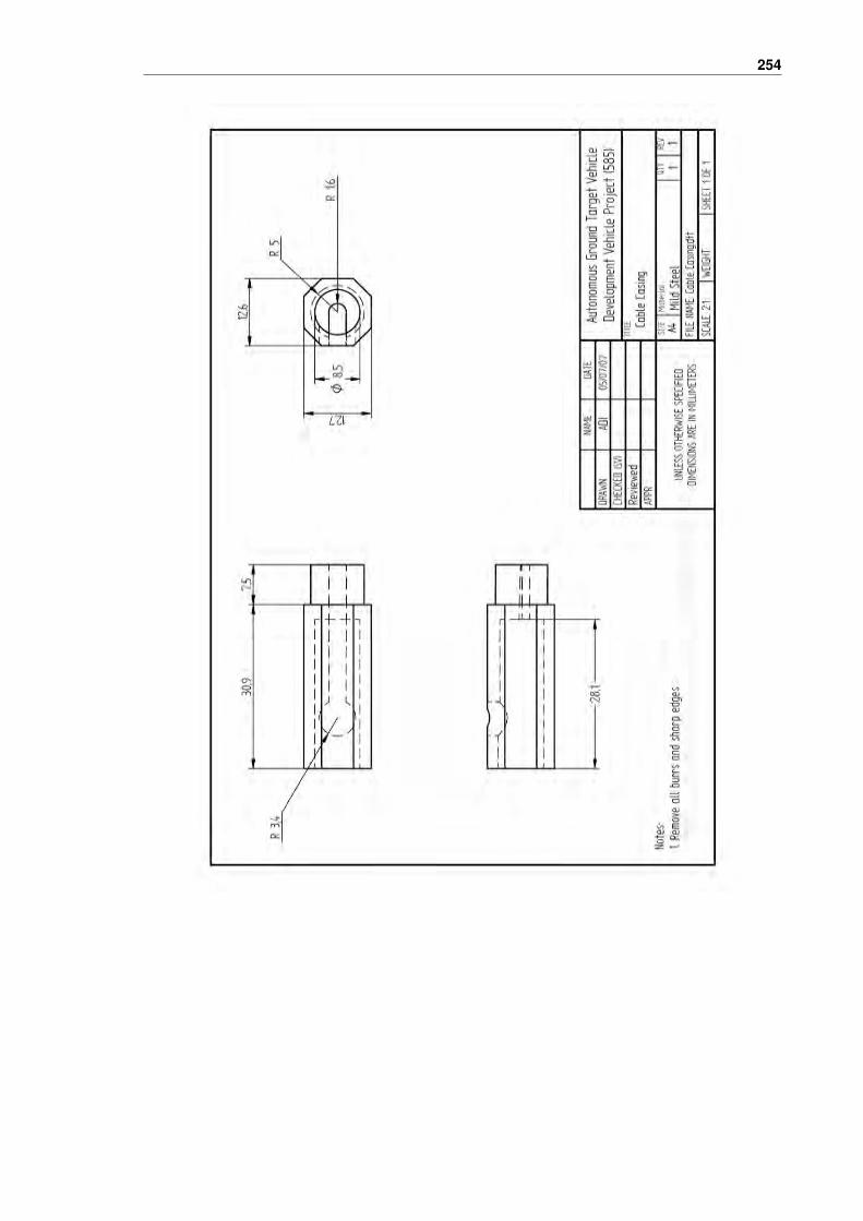
254

255 Appendix G. CAD Drawings

256

257 Appendix G. CAD Drawings

258

259 Appendix G. CAD Drawings

260

261 Appendix G. CAD Drawings
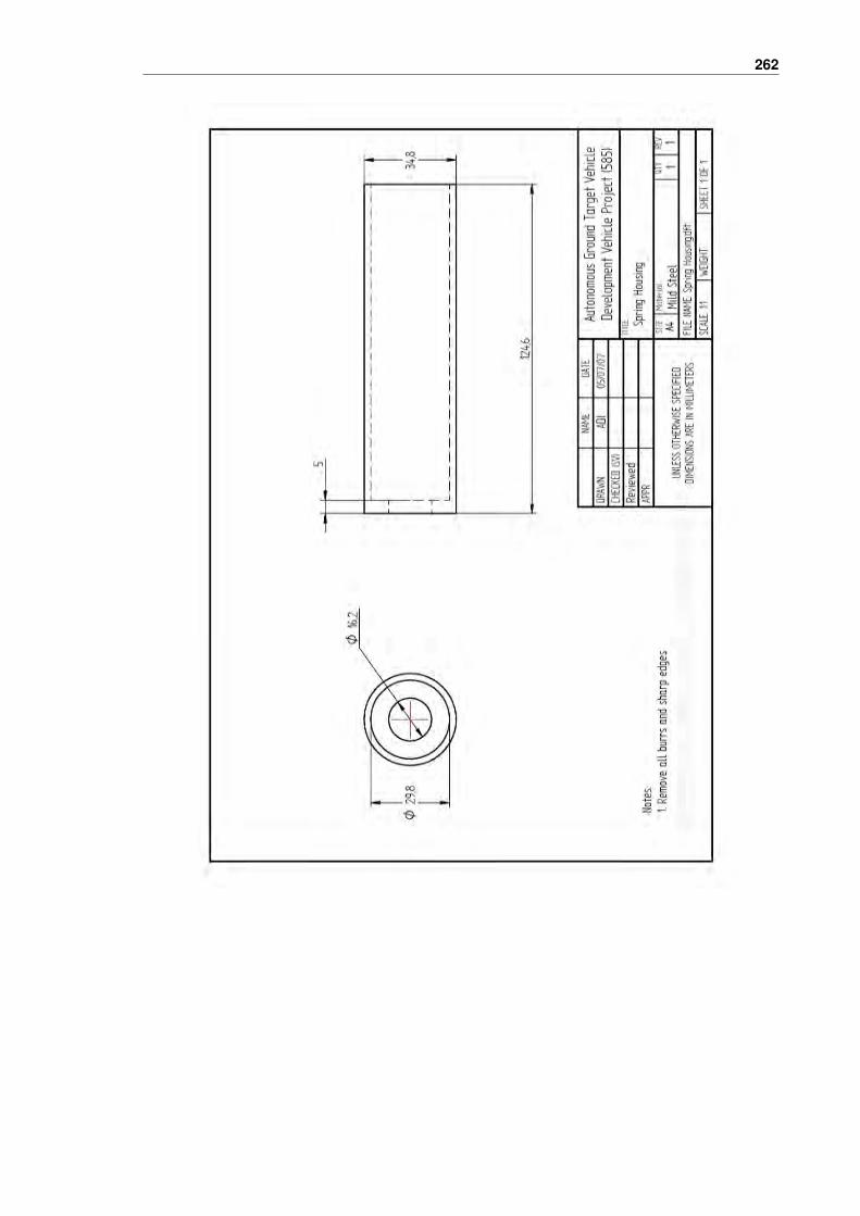
262
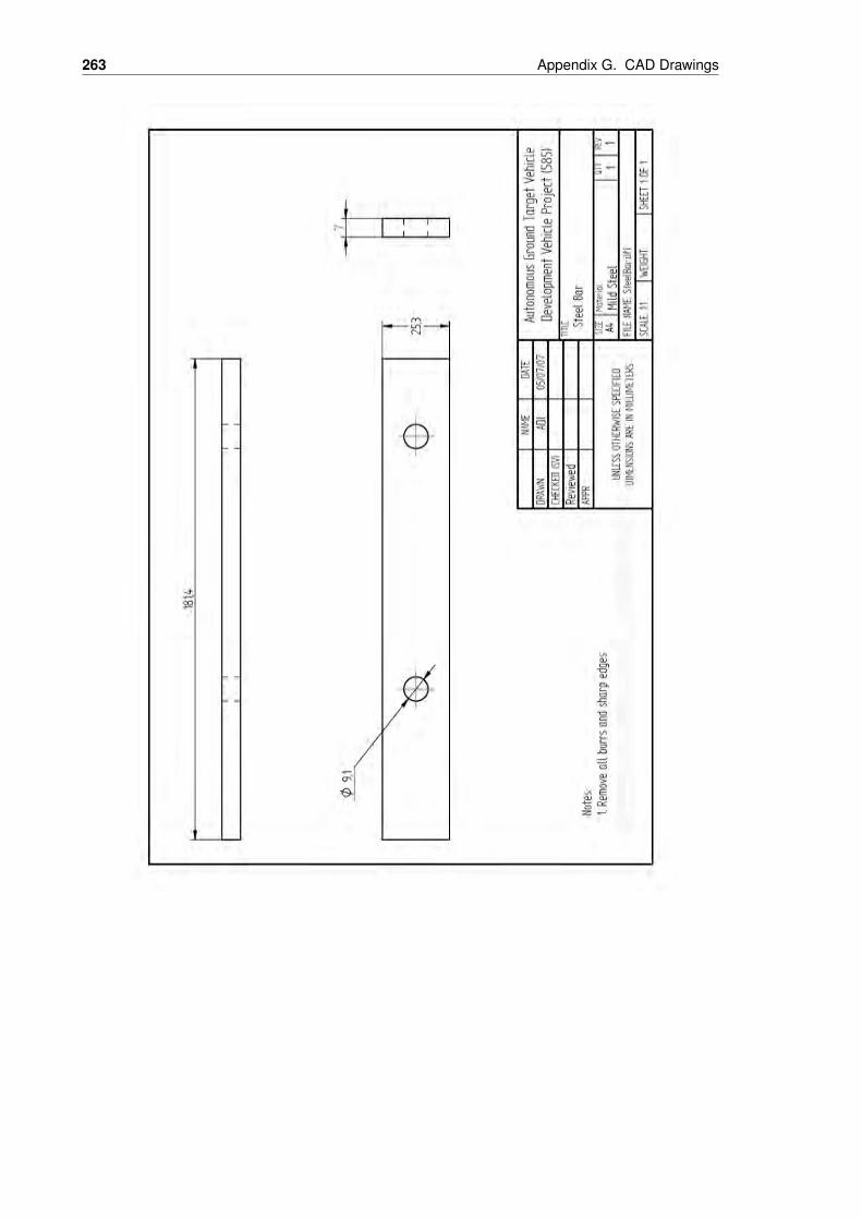
263 Appendix G. CAD Drawings

264
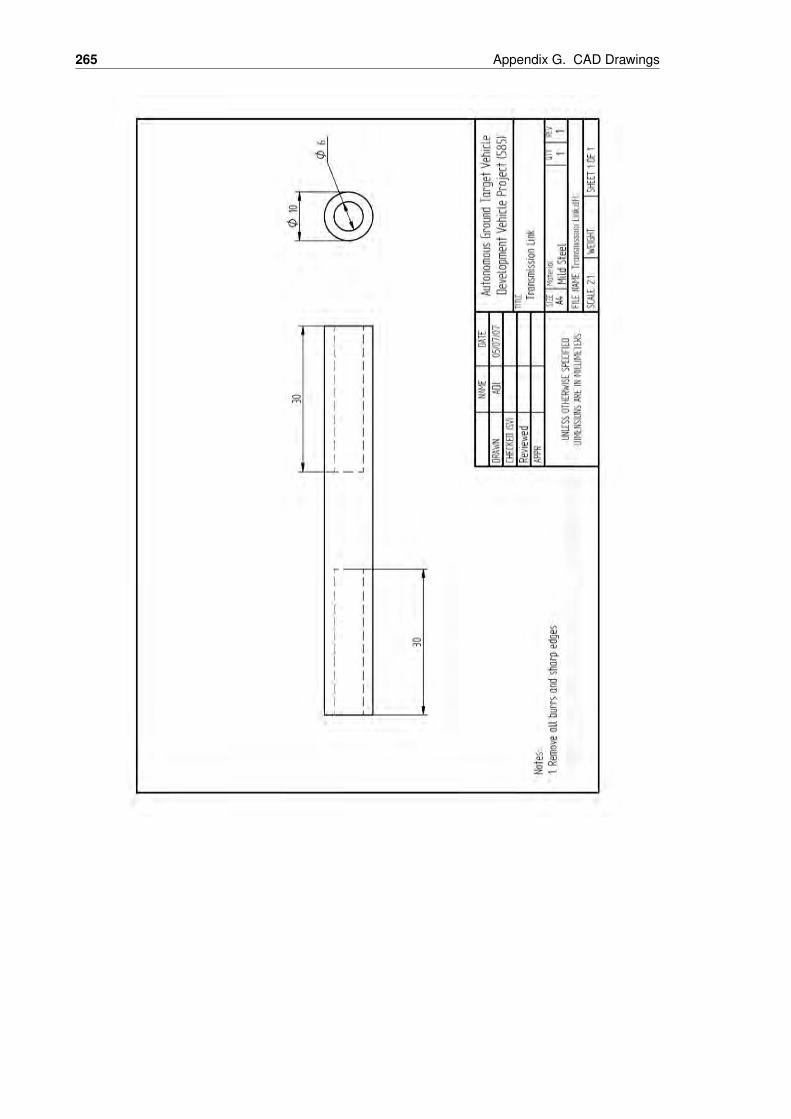
265 Appendix G. CAD Drawings
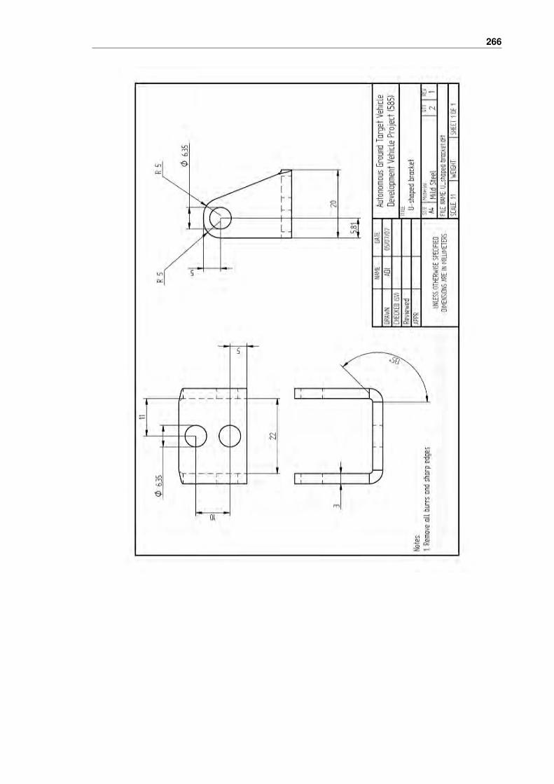
266

Appendix H
Electronic Schematic Diagrams
done
267

268

Appendix I
Selection of CommunicationHardware
done
269

270

Appendix J
Base Station User Manual
The base station software has been described in very general terms in Chapter 7 and in
Sections 3.7 and 3.8. This appendix has been aimed at providing a user manual for the use
of the base station. An overall screenshot is shown in Figure J.1 and it shows all the controls
necessary to operate the vehicle at its full potential.
Figure J.1: Screenshot of the base station software showing various dierent components onthe screen
271
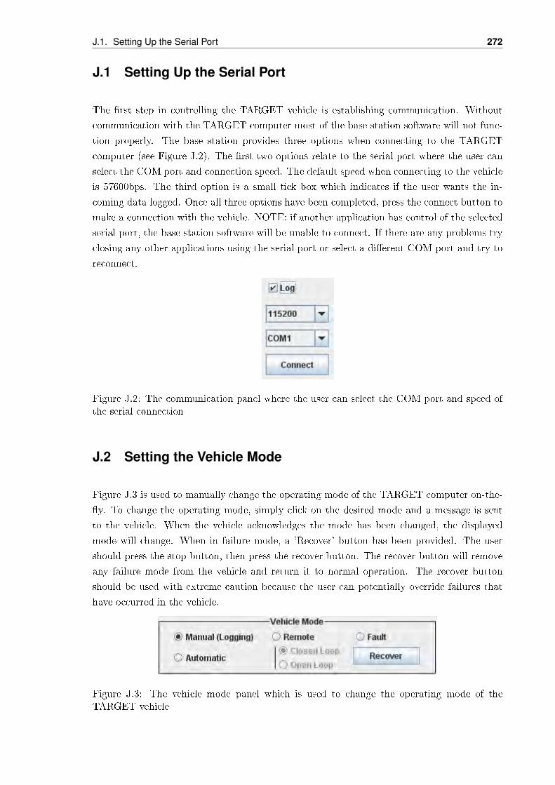
J.1. Setting Up the Serial Port 272
J.1 Setting Up the Serial Port
The rst step in controlling the TARGET vehicle is establishing communication. Without
communication with the TARGET computer most of the base station software will not func-
tion properly. The base station provides three options when connecting to the TARGET
computer (see Figure J.2). The rst two options relate to the serial port where the user can
select the COM port and connection speed. The default speed when connecting to the vehicle
is 57600bps. The third option is a small tick box which indicates if the user wants the in-
coming data logged. Once all three options have been completed, press the connect button to
make a connection with the vehicle. NOTE: if another application has control of the selected
serial port, the base station software will be unable to connect. If there are any problems try
closing any other applications using the serial port or select a dierent COM port and try to
reconnect.
Figure J.2: The communication panel where the user can select the COM port and speed ofthe serial connection
J.2 Setting the Vehicle Mode
Figure J.3 is used to manually change the operating mode of the TARGET computer on-the-
y. To change the operating mode, simply click on the desired mode and a message is sent
to the vehicle. When the vehicle acknowledges the mode has been changed, the displayed
mode will change. When in failure mode, a 'Recover' button has been provided. The user
should press the stop button, then press the recover button. The recover button will remove
any failure mode from the vehicle and return it to normal operation. The recover button
should be used with extreme caution because the user can potentially override failures that
have occurred in the vehicle.
Figure J.3: The vehicle mode panel which is used to change the operating mode of theTARGET vehicle

273 Appendix J. Base Station User Manual
J.3 Using the Map Area
The map area has the responsibility of representing the vehicle and its surroundings in a
graphical nature. The map area has many dierent functions that allow the user add, edit
and delete waypoints as well as manipulate and zoom on any path created. Zooming is
achieved by using the zoom panel (see Figure J.4). By default zooming is set to automatic.
Automatic zooming will maintain a central view of all paths and waypoints being displayed
on the screen. The zoom is updated in real time to provide the user with the best possible
view of the environment. Switching to manual zoom mode allows the user to manually zoom
in and out as well as move up, down left and right.
Figure J.4: The zoom panel which provides tools for zooming the map area
J.4 Logging Data
Data is logged automatically when the 'Log' checkbox is ticked in the communication panel
(see Figure J.2). The relevant data is automatically displayed in the status panel at all times.
J.5 Generating Pictures from the Log File
Graphs of the log le can be generated by using tools in the picture panel (see Figure J.5).
The tools allow the user to select what section of the log le to use. The user can select four
dierent options:
1. Use all data in the log le
2. Use a section (from Xms to Yms) of the log le
3. Use the rst Xms of the log le
4. Use the last Xms of the log le

J.6. Defining Background Images 274
Figure J.5: The picture panel which allows graphs to be generated from the log le
Once the selection has been made, press the 'Generate Pictures' button and wait for the
images to be craeted. The images are created and stored in the same directory as the log le
(C:\TARGET\LOG\logname) and can take several minutes to complete depending on the
number of log entries processed.
J.6 Defining Background Images
The user must supply the base station with a compatible picture format (*.jpg or *.png). The
pictures should be placed in C:\TARGET\IMAGES and be accompanied by a confuration
le named cfg.mf. The conguration le denes the coordinate systems of all the pictures
to be included in the background of the base station map area. The conguration le has a
syntax:
lename;latitude;height;longitude;width;
The latitude and longitude represent the location of the top left corner of the image. The
height and width refer to the height and width of the image represented in GPS coordinates.
An example
uni_GPS.jpg;-34.71438;-0.0090111;138.59635;0.0147444;
Multiple images can be included by dening each of the individual inages on a seperate line.
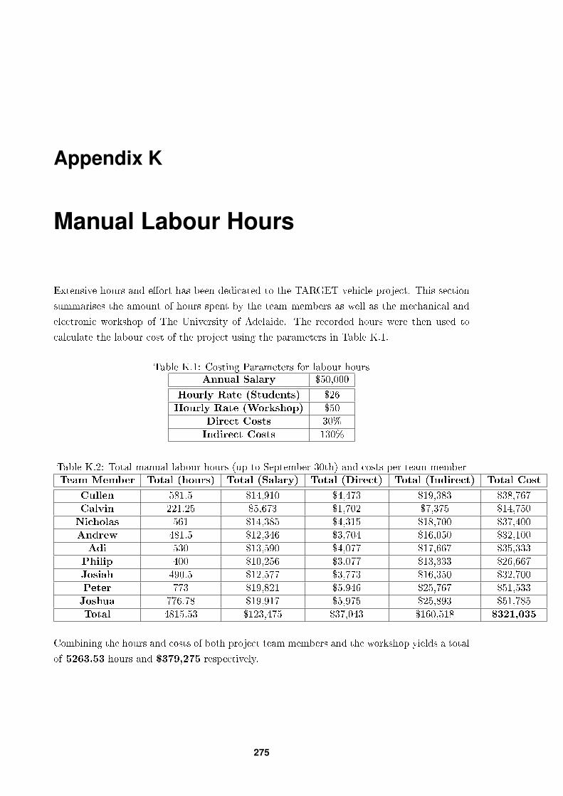
Appendix K
Manual Labour Hours
Extensive hours and eort has been dedicated to the TARGET vehicle project. This section
summarises the amount of hours spent by the team members as well as the mechanical and
electronic workshop of The University of Adelaide. The recorded hours were then used to
calculate the labour cost of the project using the parameters in Table K.1.
Table K.1: Costing Parameters for labour hoursAnnual Salary $50,000
Hourly Rate (Students) $26
Hourly Rate (Workshop) $50
Direct Costs 30%
Indirect Costs 130%
Table K.2: Total manual labour hours (up to September 30th) and costs per team memberTeam Member Total (hours) Total (Salary) Total (Direct) Total (Indirect) Total Cost
Cullen 581.5 $14,910 $4,473 $19,383 $38,767
Calvin 221.25 $5,673 $1,702 $7,375 $14,750
Nicholas 561 $14,385 $4,315 $18,700 $37,400
Andrew 481.5 $12,346 $3,704 $16,050 $32,100
Adi 530 $13,590 $4,077 $17,667 $35,333
Philip 400 $10,256 $3,077 $13,333 $26,667
Josiah 490.5 $12,577 $3,773 $16,350 $32,700
Peter 773 $19,821 $5,946 $25,767 $51,533
Joshua 776.78 $19,917 $5,975 $25,893 $51,785
Total 4815.53 $123,475 $37,043 $160,518 $321,035
Combining the hours and costs of both project team members and the workshop yields a total
of 5263.53 hours and $379,275 respectively.
275

276
Table K.3: Total manual labour hours and costs per workshopWorkshop Mechanical Electronic Total
Total (hrs) 204 244 448
Total (Salary) $10,200 $3,660 $22,400
Total (Direct) $3,060 $3,660 $6,720
Total (Indirect) $13,260 $15,860 $29,120
Total Cost $26,520 $31,720 $58,240

Appendix L
Software CD
277
Recommended