
Filter design process
In general the design of filter is composed
from three different steps
1

Filter design techniques
In the design of frequency selective filters,
the desired filter characteristics are
specified in the frequency domain in terms
of the desired magnitude and phase
response of the filter
In the filter design process, we determine
the coefficients of a causal FIR or IIR filter
that closely approximate the desired
frequency response specifications
2

Which type of filter is to be used
In general FIR filters are used in filtering
problems where a linear phase is required
IIR filters can be used if linear phase is not
required
In general IIR filter has a lower side-lobes
in the stop band than an FIR having the
same number of parameters
3
Which type of filter is to be used
If some phase distortion is tolerable then
IIR filter is preferable because its
implementation requires fewer
parameters, less memory and lower
computational complexity
A comparison between FIR and IIR filters
is made in the next slide
4

IIR versus IIR
5
Relation between IIR filter and
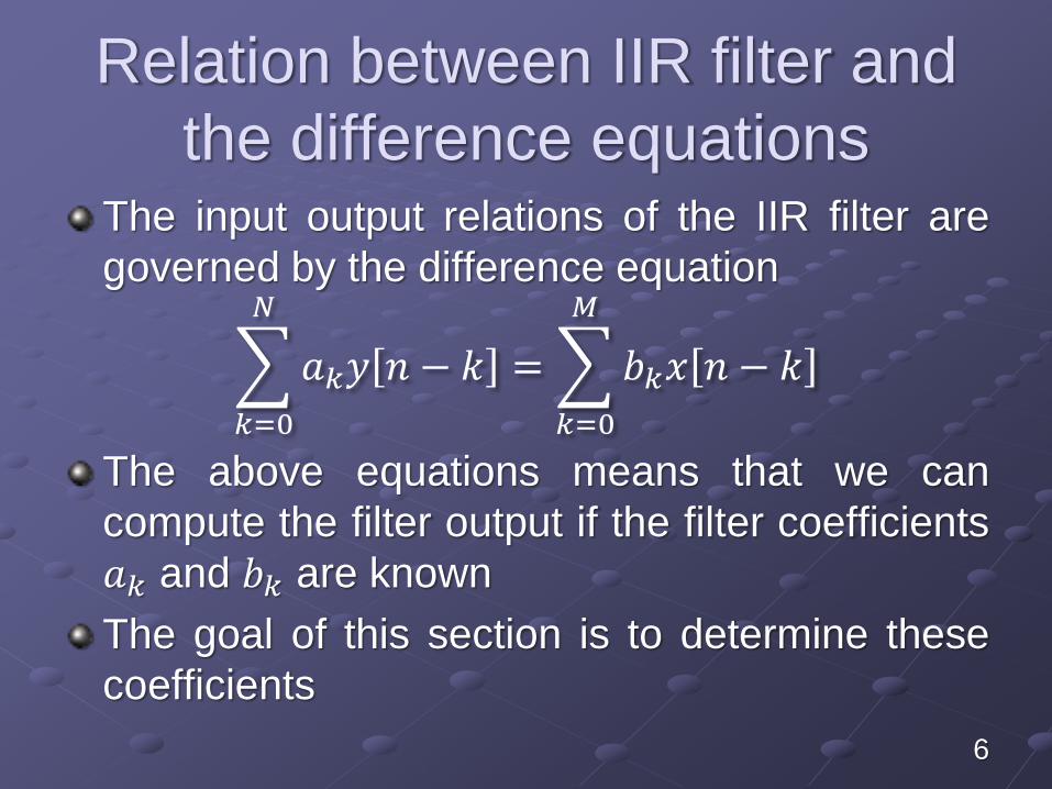
the difference equationsThe input output relations of the IIR filter are
governed by the difference equation
𝑘=0
𝑁
𝑎𝑘𝑦 𝑛 − 𝑘 =
𝑘=0
𝑀
𝑏𝑘𝑥 𝑛 − 𝑘
The above equations means that we can
compute the filter output if the filter coefficients
𝑎𝑘 and 𝑏𝑘 are known
The goal of this section is to determine these
coefficients
6

Relation between IIR filter and
the difference equationsIf we apply the z transform to the LCCD
difference equation which describes the
IIR filter we got the discrete filter system
function given by
𝐻 𝑧 = 𝑘=0𝑀 𝑏𝑘𝑧
−𝑘
1 + 𝑘=1𝑁 𝑎𝑘𝑧
−𝑘
It can be noticed that 𝐻(𝑧) is a rational
function
7

Causality and its implications
All ideal filters are non causal
Non causal means that these filters are
not physically realizable
To illustrate this concept let us consider an
ideal low pass filer
The frequency response of the filter is
given by 𝐻 𝜔 =1 𝜔 ≤ 𝜔𝑐0 𝜔𝑐 < 𝜔 < 𝜋
8

Causality and its implications
The impulse response of the filter is given
by ℎ 𝑛 =𝜔𝑐
𝜋
𝑠𝑖𝑛𝜔𝑐𝑛
𝜔𝑐𝑛
Typical plot of the ideal LPF filter for 𝜔𝑐 =𝜋
4
is shown below
9

Causality and its implications
From the plot of ℎ[𝑛] it is clear that ℎ 𝑛 ≠0 for 𝑛 < 0 which means that the filter is
not causal
If the filter is not causal this means that the
filter output samples 𝑦[𝑛] depends on the
future values of the input 𝑥[𝑛 + 1], 𝑥[𝑛 +2] which is impossible to estimate
10

Processing continuous time
signal with digital filterConsider a discrete-time filter is to be used
to low pass filter a continuous time signal
The complete system may be presented
as shown below
11
Determining specifications for a
discrete time filter
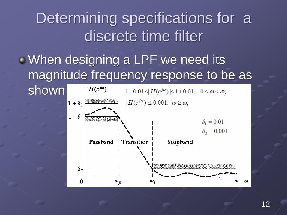
When designing a LPF we need its
magnitude frequency response to be as
shown
12

Design of discrete time IIR filters
from continuous time filters
The traditional approach to design IIR
filters involves the transformation of a
continuous-time filter into a discrete-time
filter meeting prescribed specifications
This design procedure can be achieved by
finding the system function 𝐻𝑐(𝑠) or the
impulse response of the continuous filter
ℎ𝑐(𝑡)
13

Design of discrete time IIR filters
from continuous time filters
There are four well known analog filters
used in the design of IIR digital filters
these are
Butterworth
Chebyshev I
Chebyshev II
Elliptic
14

Design of discrete time IIR filters
from continuous time filters
The system function 𝐻(𝑧) or the impulse
response ℎ 𝑛 for the discrete-time filter is
obtained by using either
Impulse invariance method
Bilinear transformation
15

IIR filter design by Impulse
invarianceIn the impulse invariance method we can
design an IIR filter by sampling the
impulse response of analog filter
according to
ℎ 𝑛 = 𝑇𝑑ℎ𝑐 𝑛𝑇𝑑Where 𝑇𝑑 represents the sampling interval
16

IIR filter design by Impulse
invarianceIf the continuous time filter is band limited,
so that
𝐻𝑐 𝑗Ω = 0 Ω ≥𝜋
𝑇𝑑
𝐻 𝑒𝑗𝜔 = 𝐻𝑐(𝑗𝜔
𝑇𝑑) 𝜔 ≤ 𝜋
17

IIR filter design by Impulse
invariance
The discrete-time filter and the continuous
time filter frequency responses are related
by a linear scaling of the frequency axis
which is given by 𝜔 = Ω𝑇𝑑 for 𝜔 ≤ 𝜋
Where 𝜔 is the discrete frequency axis
and Ω is the continuous frequency axis
18

Practical IIR filter and aliasing
Any practical continuous filter can not be
exactly band limited
This means that the sampling process will
cause interference between successive
samples which causes aliasing as shown
19

Practical IIR filter and aliasing
The aliasing problem makes the impulse
invariance method not a suitable method for
the design of high pass filters
However if the continuous time filter
approaches zero at high frequencies, the
aliasing is negligible and can be ignored
20

IIR filter and continuous to discrete
system function transformation
Consider the system function of the
continuous-time filter expressed in terms of
partial fractions as shown below
The corresponding impulse response is
(inverse Laplace transform)
𝑁 represents the number
of poles
21

IIR filter and continuous to discrete
system function transformation
The impulse response of the discrete time filter
obtained by sampling 𝑇𝑑ℎ𝑐(𝑡) as shown
The system function of the discrete time filter is
22

IIR filter and continuous to discrete
system function transformation
If we compare the system function for both
continuous time 𝐻𝑐 𝑠 and discrete time 𝐻(𝑧)system function, we observe that a pole at
𝑠 = 𝑠𝑘 in the S- plane transforms to a pole at
𝑧 = 𝑒𝑠𝑘𝑇𝑑 in the z plane
Also the coefficients in the partial fraction for
both 𝐻𝑐 𝑠 and 𝐻(𝑧) are equal, except for the
scaling multiplier 𝑇𝑑
23
IIR filter and continuous to discrete
system function transformation
Note that 𝑠𝑘 is acomplex number which can be
written as 𝑠𝑘 = 𝜎 + 𝑗𝜔 this means that 𝑧 =𝑒𝜎𝑇𝑑𝑒𝑗𝜔𝑇𝑑
If the real par of 𝑠𝑘 is less than zero (𝜎 negative),
then 𝑧 < 1 , the corresponding pole in the
discrete time filter falls inside the unit circle
This means that the causal discrete time filter is
stable
24

Example 1
Example 1 convert the analog filter defined
by the system function 𝐻𝑎 𝑠 =1
(𝑠+0.1)2+9into
a digital IIR filter by means of impulse
invariance method
25

Example1 solution
Solution
Since the filter system function 𝐻𝑐 𝑠 for the
continuous filter is given we can find
𝐻(𝑧) directly through the partial fraction (no
need to go back to the time domain and then
use sampling)
From 𝐻𝑐 𝑠 we can find that the filter has two
poles located at
𝑠1 = −0.1 + 𝑗3 and 𝑠2 = −0.1 − 𝑗3
26

Example1 solution
Solution
If we analyze 𝐻𝑐 𝑠 by the partial fraction
we get
To find 𝐻(𝑧) we use the expression
developed in slide 23
27

Example1 solution
If we plot the poles and zeros of the
previous example we can see that 𝜎 < 0and both poles are located in the left side
of the s plane as shown below
28

Example 1 solution
If we manipulate 𝐻(𝑧) expression we find that
𝐻(𝑧) can be written as
If we compare this expression for 𝐻(𝑧) with
𝐻 𝑧 = 𝑘=0𝑀 𝑏𝑘𝑧
−𝑘
1+ 𝑘=1𝑁 𝑎𝑘𝑧
−𝑘 we can find the filter
coefficients are
𝑏0 = 1, 𝑏1 = −𝑒−0.1𝑇𝑑cos(3𝑇𝑑), 𝑎0 = 1, 𝑎1 =
− 2𝑒−0.1𝑇𝑑 cos 3𝑇𝑑 , 𝑎2 = 𝑒−0.2𝑇𝑑,
29
2

Example 2
The system function of a discrete time
system is 𝐻 𝑧 =1
1−𝑒−0.2𝑧−1+
1
1−𝑒−0.4𝑧−1,
determine the filter coefficients
30

Example 2 solution
Note the discrete time system can be
rewritten as 𝐻 𝑧 =2− 𝑒−0.4+𝑒−0.2 𝑧−1
1− 𝑒−0.4+𝑒−0.2 𝑧−1+𝑒−0.6𝑧−2
If we compare this expression for 𝐻(𝑧) with
𝐻 𝑧 = 𝑘=0𝑀 𝑏𝑘𝑧
−𝑘
1+ 𝑘=1𝑁 𝑎𝑘𝑧
−𝑘 we can find the filter
coefficients are
𝑏0 = 2 , 𝑏1 = 𝑒−0.4 + 𝑒−0.2 , 𝑎0 = 1 , 𝑎1 =
− 𝑒−0.4 − 𝑒−0.2, 𝑎2 = 𝑒−0.6
31

Example 3
Design a Butterworth filter whose continuous
frequency response is given by
𝐻𝑐(𝑗Ω)2 =
1
1+Ω
Ω𝑐
2𝑁
using the impulse invariance method
The filter specifications are
32

Example 3 solution
Solution
Since the parameter 𝑇𝑑 cancels in the impulse
invariance procedure we can select 𝑇𝑑 = 1 ,
therefore Ω = 𝜔
In order to deign the filter we need to transform
the discrete filter specifications to specifications
on the continuous time filter
33

Example 3 solution
Solution
The continuous time filter specifications became
The filter magnitude at the pass band and stop
band frequencies is given by
34

Example 3 solution
Solution
From the above magnitude conditions, the
magnitude squared of the continuous filter at
both the pass and stop bands is given by
0.89125 2 =1
1+0.2𝜋
Ω𝑐
2𝑁
0.17783 2 =1
1+0.3𝜋
Ω𝑐
2𝑁
35

Example 3 solution
Solution
If we solve the above two equations for 𝑁 and
Ω𝑐 we got 𝑁 = 5.8858 ≈ 6 and Ω𝑐 = 0.7032
Since 𝑁 = 6 then the filter has 12 poles of the
magnitude squared function 𝐻𝑐 𝑠 𝐻𝑐 −𝑠 =1
1+𝑆
Ω𝑐
2𝑁
The poles can easily be found by using the
following matlab commands
36

Example 3 solution
𝑎 = 1
b=[68.399 0 0 0 0 0 0 0 0 0 0 0 1]
[𝑧 𝑝 𝑘] = 𝑡𝑓2𝑧𝑝(𝑎, 𝑏)
37

Example 3 solution
Solution
The poles are uniformly
distributed in angle of360°
12= 30° on a circle of
radius Ω𝑐 = 0.7032 as
shown
38

Example 3 solution
Solution
The poles that describe a stable system are
those poles located in the left side of the s-plane
The number of these poles is 6 and one solution
for these poles is on the assumption that the first
pole located a at an angle of 105°
39
Example 3 solution
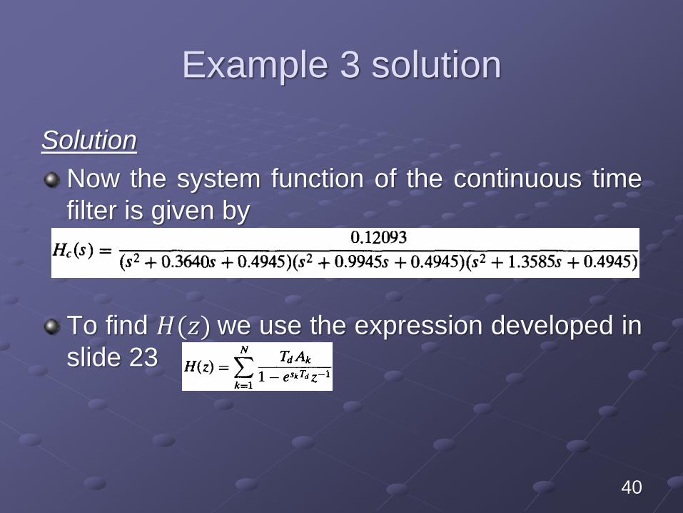
Solution
Now the system function of the continuous time
filter is given by
To find 𝐻(𝑧) we use the expression developed in
slide 23
40

Example 3 solution
Solution
In order to find the filter coefficients again we need
to write 𝐻(𝑧) as a rational function and then find
the coefficients as we have did in the previous two
examples
41

Impulse invariance summery
To summarize, the impulse invariance method maps
the s-plane to the z-plane by sampling the impulse
response of continuous (analog) time filter
Impulse invariance suffers from aliasing problem
and therefore is not suitable for HPF design
42

Impulse invariance summery
In order to find the filter coefficients follow these steps
1. find 𝐻𝑐 𝑠 , expand it in partial fraction, find the poles
of 𝐻𝑐 𝑠
2. Next find the discrete system function according to
𝐻 𝑧 = 𝑘=1𝑁 𝑇𝑑𝐴𝑘
1−𝑒𝑠𝑘𝑇𝑑𝑧−1
3. Convert 𝐻(𝑧) to rational function
4. Compare the rational expression for 𝐻(𝑧) with
𝐻 𝑧 = 𝑘=0𝑀 𝑏𝑘𝑧
−𝑘
1+ 𝑘=1𝑁 𝑎𝑘𝑧
−𝑘 and determine the coefficients
accordingly
43

Bilinear transformation
The bilinear transformation is an algebraic
transformation between the 𝑠 and 𝑧 planes
Bilinear transformation maps the entire 𝑗Ω-axis in the s-plane to one revolution of the
unit circle in the z-plane
Bilinear transformation avoids the aliasing
problem associated with time invariant
approach
44

Bilinear transformation
The bilinear transformation corresponds to
replacing 𝑠 by
𝑠 =2
𝑇𝑑
1 − 𝑧−1
1 + 𝑧−1
This means that the discrete and
continuous system functions are related by
𝐻 𝑧 = 𝐻𝑐2
𝑇𝑑
1 − 𝑧−1
1 + 𝑧−1
45

Bilinear transformation
To develop the properties of the algebraic
transformation we solve for 𝑧 to obtain
𝑧 =2
𝑇𝑑
1 +𝑇𝑑2𝑠
1 −𝑇𝑑2𝑠
Substituting 𝑠 = 𝜎 + 𝑗𝜔, we got
𝑧 =1 + 𝜎𝑇𝑑2+ 𝑗Ω𝑇𝑑2
1 − 𝜎𝑇𝑑2− 𝑗Ω𝑇𝑑2
46

Bilinear transformation
Again as in the time invariant procedure, if 𝜎 <0, 𝑧 < 1, for any value of Ω
This means the poles fall in the left half of the s-
plane or inside the unit circle of the z-plane,
which means that the system is stable
Similarly if of 𝜎 > 0, 𝑧 > 1, for any value of Ω
The poles fall in the right half of the s-plane or
outside the unit circle of the z-plane, which
means that the system is unstable
47

Bilinear transformation
In order to show that the 𝑗Ω-axis of the s-plane
maps onto the unit circle, substitute 𝜎 = 0 into
𝑧 =1+𝜎𝑇𝑑2+𝑗Ω𝑇𝑑2
1−𝜎𝑇𝑑2−𝑗Ω𝑇𝑑2
and simplify the expression we
got
𝑧 =1 + 𝑗Ω
𝑇𝑑2
1 − 𝑗Ω𝑇𝑑2
Recall that 𝑧 = 𝑒𝜎𝑒𝑗𝜔 = 𝑒𝑗𝜔
48

Bilinear transformation
The expression for 𝑠 =2
𝑇𝑑
1−𝑧−1
1+𝑧−1can be
rewritten as s =2
𝑇𝑑
1−𝑒−𝑗𝜔
1+𝑒−𝑗𝜔or equivalently
𝑠 = 𝜎 + 𝑗Ω =2
𝑇𝑑
2𝑒−𝑗𝜔2 sin
𝜔
2
2𝑒−𝑗𝜔2 cos
𝜔
2
=2𝑗
𝑇𝑑tan
𝜔
2
From which we can conclude that
Ω =2
𝑇𝑑tan
𝜔
2or 𝜔 = 2𝑡𝑎𝑛−1
Ω𝑇𝑑
2
49

Mapping between the z-plane
and the s-planeThe properties of the bilinear transformation as
mapping from the s-plane to the z-plane are
illustrated graphically as shown below
50

Axis mapping notes
Note that the Bilinear transformation maps
the range of continuous frequencies 0 ≤Ω ≤ ∞ maps to 0 ≤ 𝜔 ≤ 𝜋 on the discrete
frequency axis
Also the range of continuous frequencies
−∞ ≤ Ω ≤ 0 maps to −𝜋 ≤ 𝜔 ≤ 0 on the
discrete frequency axis as illustrated in the
next slide
51

Axis mapping notes
52
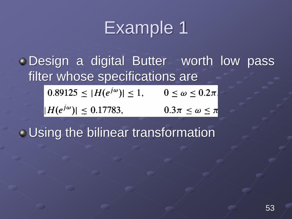
Example 1
Design a digital Butter worth low pass
filter whose specifications are
Using the bilinear transformation
53

Example 1 solution
The design procedure starts by reflecting the
specifications of the discrete filter to
specifications of the digital filter as shown
Let 𝑇𝑑 = 1
54

Example 1 solution
The magnitude of the filter at the pass
band frequency Ω𝑝 = 2 tan0.2𝜋
2is given
by
Also note that the magnitude of the filter at
the stop band Ω𝑠 = 2 tan0.3𝜋
2is given by
55

Example 1 solution
By substituting the values of Ω𝑝 and Ω𝑠 in
the magnitude squared of the Butterworth
filter we got the following equations
By solving these two equations for Ω𝑐 and
𝑁 we got 𝑁 = 5.305 ≈ 6 and Ω𝑐 = 0.766
56

Example 1 solution
If we plot the poles of 𝐻𝑐 𝑠2 of the filter
we got the following graph
57

Example 1 solution
From the pole plot it can be shown that
58

Example 2
Design a single pole low pass digital filter
with a 3-dB bandwidth of 0.2𝜋, using the
bilinear transformation applied to the
analog filter defined by 𝐻 𝑠 =Ω𝑐
𝑠+Ω𝑐where
Ω𝑐 is the 3-dB bandwidth of the filter
59

Example 2 solution
By using the linear transformation we have
Ω𝑐 =2
𝑇𝑑tan
0.2𝜋
2=0.65
𝑇𝑑
The system function of the analog filter can
be written as 𝐻 𝑠 =
0.65
𝑇𝑑
𝑠+0.65
𝑇𝑑
By substituting 𝑠 =2
𝑇𝑑
1−𝑧−1
1+𝑧−1, we got the
discrete system function as
60

Example 2 solution
𝐻 𝑧 =
0.65
𝑇𝑑
21−𝑧−1
1+𝑧−1+0.65
𝑇𝑑
= 0.2451+𝑧−1
1−0.509𝑧−1
61
IIR filter design in MATALB
We have seen from the previous discussion both
the impulse invariance and bilinear
transformations needs too many computations
A simpler way to design an IIR filter can be done
easily with the aid of MATLAB
It is easy to show this by an example
62

IIR filter design in MATLAB
Design a band pass filter with the following
specifications
Pass band frequencies from 1000 to 2000 Hz
The stop bands starting 500 Hz away on either side
A 10 kHz sampling frequency
At most 1 dB of pass band ripple and at least 60 dB of
stop band attenuation
63

IIR filter design in MATLAB
Solution
In order to design the filter we need to specify its
coefficients
This can be achieved by using the following
statements in MATLAB
𝑓𝑠 = 10 𝑘𝐻𝑧 % Sampling frequency
𝑓𝑝1 = 1 𝑘𝐻𝑧 % The first band pass frequency
𝑓𝑝2 = 2 𝑘𝐻𝑧 % The second band pass frequency
𝑓𝑠1 = 500 𝐻𝑧 % The first stop band frequency
𝑓𝑠2 = 2500 𝐻𝑧 % The second stop band frequency
64

IIR filter design in MATLAB
𝑅𝑝 = 1 𝑑𝐵 % The ripple in the pass band
𝑅𝑆 = 60 𝑑𝐵 % The attenuation in the stop band
The filter order and normalized frequencies can be
computed by using the following statement
[𝑛,𝑊𝑛] = 𝑏𝑢𝑡𝑡𝑜𝑟𝑑𝑓𝑝1 𝑓𝑝2
𝑓𝑠,𝑓𝑠1 𝑓𝑠2
𝑓𝑠, 𝑅𝑝, 𝑅𝑠
The filter coefficients can be computed from the
following statements
𝑏, 𝑎 = 𝑏𝑢𝑡𝑡𝑒𝑟 𝑛,𝑊𝑛 ;
65

IIR filter design in MATLAB
More examples to design IIR filter is by the use of these
statements [𝑏, 𝑎] = 𝑏𝑢𝑡𝑡𝑒𝑟(𝑛,𝑊𝑛, 𝑜𝑝𝑡𝑖𝑜𝑛𝑠)
[𝑏, 𝑎] = 𝑏𝑢𝑡𝑡𝑒𝑟(5,0.4); % Lowpass Butterworth
[𝑏, 𝑎] = 𝑐ℎ𝑒𝑏𝑦1(𝑛, 𝑅𝑝,𝑊𝑛, 𝑜𝑝𝑡𝑖𝑜𝑛𝑠)
[𝑏, 𝑎] = 𝑐ℎ𝑒𝑏𝑦1(4,1, [0.4 0.7]); % Bandpass Chebyshev Type I
[𝑏, 𝑎] = 𝑐ℎ𝑒𝑏𝑦2(𝑛, 𝑅𝑠,𝑊𝑛, 𝑜𝑝𝑡𝑖𝑜𝑛𝑠)
[𝑏, 𝑎] = 𝑐ℎ𝑒𝑏𝑦2(6,60,0.8, ′ℎ𝑖𝑔ℎ′); % Highpass Chebyshev Type II
[𝑏, 𝑎] = 𝑒𝑙𝑙𝑖𝑝(𝑛, 𝑅𝑝, 𝑅𝑠,𝑊𝑛, 𝑜𝑝𝑡𝑖𝑜𝑛𝑠)
[𝑏, 𝑎] = 𝑒𝑙𝑙𝑖𝑝(3,1,60, [0.4 0.7], ′𝑠𝑡𝑜𝑝′); % Bandstop elliptic
66

Filter design in MATLAB
We can design IIR or FIR filters in MATALB
using the filter design and analysis tool
FDATOOL
In the command window of MATLAB type
FDATOOL
A window the filter design window will appear as
shown in the next slide
67

68

Using FDATOOL
To design a filter, you need to specify the
sampling rate, pass and stop band frequencies
You can also determine the filter type,
implementation, FIR or IIR
Once the filter is designed you can view or
export the filter coefficients to workspace or file
using the command file as illustrated in the next
slide
69

Exporting filter coefficients
70
Recommended


