. RESEARCH PAPER .
SCIENCE CHINAInformation Sciences
May 2014, Vol. 57 052104:1–052104:21
doi: 10.1007/s11432-014-5082-z
c© Science China Press and Springer-Verlag Berlin Heidelberg 2014 info.scichina.com link.springer.com
Feature-aware regularizationfor sparse online learning
OIWA Hidekazu1∗, MATSUSHIMA Shin1 & NAKAGAWA Hiroshi1,2
1Graduate School of Information Science and Technology, The University of Tokyo, Tokyo 113-8654, Japan;2Information Technology Center, The University of Tokyo, Tokyo 113-8654, Japan
Received August 31, 2013; accepted November 24, 2013
Abstract Learning a compact predictive model in an online setting has recently gained a great deal of at-
tention. The combination of online learning with sparsity-inducing regularization enables faster learning with a
smaller memory space than the previous learning frameworks. Many optimization methods and learning algo-
rithms have been developed on the basis of online learning with L1-regularization. L1-regularization tends to
truncate some types of parameters, such as those that rarely occur or have a small range of values, unless they
are emphasized in advance. However, the inclusion of a pre-processing step would make it very difficult to pre-
serve the advantages of online learning. We propose a new regularization framework for sparse online learning.
We focus on regularization terms, and we enhance the state-of-the-art regularization approach by integrating
information on all previous subgradients of the loss function into a regularization term. The resulting algorithms
enable online learning to adjust the intensity of each feature’s truncations without pre-processing and eventually
eliminate the bias of L1-regularization. We show theoretical properties of our framework, the computational
complexity and upper bound of regret. Experiments demonstrated that our algorithms outperformed previous
methods in many classification tasks.
Keywords online learning, supervised learning, sparsity-inducing regularization, feature selection, sentiment
analysis
Citation Oiwa H, Matsushima S, Nakagawa H. Feature-aware regularization for sparse online learning. Sci
China Inf Sci, 2014, 57: 052104(21), doi: 10.1007/s11432-014-5082-z
1 Introduction
Online learning is a learning framework where a prediction and parameter update take place in a sequential
setting each time a learner receives one datum. Online learning is beneficial for learning from large-scale
data in terms of used memory space and computational complexity. If training data is very large, many
batch algorithms cannot derive a global optimal solution within a reasonable amount of time because
the computational cost is very high. If all instances cannot be simultaneously loaded into the main
memory, optimization in batch learning requires some sort of reformulation in order to arrive at an exact
solution [1]. Many online learning algorithms update predictors on the basis of only one new instance.
This means that online learning runs faster and uses a smaller memory space than batch learning does.
∗Corresponding author (email: [email protected])
Oiwa H, et al. Sci China Inf Sci May 2014 Vol. 57 052104:2
Online learning algorithms are especially efficient on datasets where the dimension of instances or number
of instances is very large. Many algorithms have been transformed into online ones for their ease of
handling large-scale data.
Regularization is a generalization technique to prevent over-fitting of previously received data. L1-
regularization is a well-known method of deriving a compact predictive model. The functionality of
L1-regularization is to eliminate parameters that are insignificant for prediction on the fly. A compact
model is able to reduce the computational time and required memory space for making predictions because
it deals with a smaller number of parameters. In addition, L1-regularization has a generalization effect
for preventing over-fitting to the training data.
Online learning with L1-regularization is currently being studied as a way of solving large-scale opti-
mization problems. Some novel frameworks have been developed in this field. Most of these works are
subgradient-based; that means the update is performed by calculating the subgradients of loss functions.
Subgradient-based online learning has high computational efficiency and high predictive performance.
There are three major subgradient-based algorithms for sparse online learning:
1) COMID (Composite Objective MIrror Descent) [2,3];
2) RDA (Regularized Dual Averaging) [4];
3) FTPRL (Follow-The-Proximally-Regularized-Leader) [5,6];
However, these subgradient-based online algorithms do not consider information on features. The plain
L1-regularization makes parameters closer to 0 without considering their range of values or frequency of
occurrences. As a result, most unemphatic features are easily truncated, even though such features are
crucial for making a prediction. The occurrence frequency and value range are not usually uniform in
tasks such as natural language processing and pattern recognition. Some techniques to emphasize them
have been developed to retain such features in the predictive model1). However, these methods must
load all data and sum up the occurrence counts of each feature before starting to learn and hence are
pre-processings. As the name implies, pre-processing poisons the essence of online learning wherein the
data are sequentially processed and there is no hypothesis that we can sum up feature occurrence counts
by using all data. The previous work however has not dealt with these challanges in any detail.
We propose a new sparsity-inducing regularization framework for subgradient-based online learning.
Our framework enables us to eliminate the bias for retaining informative features in an online setting
without any pre-processing. The key idea behind our framework is to integrate the absolute values of
the subgradient of loss functions into the regularization term. We call this framework feature-aware reg-
ularization for sparse online learning. Our framework can dynamically weaken truncation effects on rare
features and thereby obtain a set of important features regardless of their occurrence frequency or value
range. Our extension can be applied to many subgradient-based online learning, such as COMID, RDA,
and FTPRL. We show three applications of our framework in this paper, FR-COMID (Feature-aware Reg-
ularized COMID), which is an extension of COMID, FRDA (Feature-aware Regularized Dual Averaging),
which is an extension of RDA, and FTPFRL (Follow-The-Proximally-Feature-aware-Regularized-Leader),
which is an extension of FTPRL. We also analyzed the theoretical aspects of our framework. As a result,
we derived the same computational cost and the regret upper bound as those for the original algorithms.
Finally, we evaluated our framework in several experiments. The results revealed that our framework
improved state-of-the-art algorithms on most datasets in terms of prediction accuracy and sparsity.
This paper is constituted as follows. Section 2 introduces the basic framework of subgradient-based
online learning and describes the three major sparse online learning algorithms, COMID, RDA, and
FTPRL. Section 3 introduces the previous work done on sparse online learning. In Section 4, we propose
our new sparsity-inducing regularization framework, called feature-aware regularization. We show some
common examples that the previous work causes problems in sparse online learning. As a solution to
these problems, we propose a new framework for the three previous algorithms. For each algorithm, we
derive closed form update formula. Section 5 discusses the upper bound of regret for our algorithms,
and Section 6 describes the results of several experiments. Section 7 concludes the discussion of our
framework.
1) For example, TF-IDF [7] in tasks on natural language processing.
Oiwa H, et al. Sci China Inf Sci May 2014 Vol. 57 052104:3
Table 1 Notation
λ Scalar
|λ| Absolute value
a Vector
a(i) ith entry of vector a
A Matrix
I Identity matrix
A(i,j) (i,j)th entry of matrix A
‖a‖p Lp norm
〈a, b〉 Inner product
Rn n-dimensional Euclidean space
domf Domain of function f
sgn(·) Sign of a real number
argmin f Unique point for minimizing function f
Argmin f Set of minimizing points of function f
∂f(a) Differential of function f at a
∇f(a) Gradient of function f (differentiable)
Bψ(·, ·) Bregman divergence
2 Subgradient-based online learning
Before explaining the three major sparse online learning algorithms, we will describe the notation used
in this paper and the problem setting for subgradient-based online learning.
2.1 Notation
Our notation to formally describe the problem setting is summarized in Table 1. Scalars are denoted
in lowercase italic letters, e.g., λ, and the absolute value of a scalar is |λ|. Vectors are in lowercase
bold letters, such as a. Matrices are in uppercase bold letters, e.g., A. I is the identity matrix. ‖a‖prepresents the Lp norm of a vector a, and 〈a, b〉 denotes the inner product of two vectors a, b. Rn is an
n-dimensional Euclidean space and R+ is a one-dimensional non-negative Euclidean space. Let domf be
the domain of function f . A function sgn is defined as sgn(λ) = λ/|λ| where λ is a real number (If λ = 0,
sgn(λ) = 0). Let argmin f be a unique point at which function f is a minimum. Let Argmin f be the set of
minimizing points of a function f . ∂f(a) is the subdifferential of function f , where the subdifferential of
f at a means the set of all vectors g ∈ Rn satisfying ∀b, f(b) � f(a)+〈g, b−a〉.We call a subdifferential
of a function f at a a subgradient of a function f at a. Any g is a subgradient such that g ∈ ∂f(a).
Even if f is non-differentiable, at least one subgradient exists when f is convex. A function f is convex
when f satisfies the following inequality: ∀t ∈ [0, 1], a, b, f (ta+ (1− t)b) � tf(a) + (1− t)f(b). When
a function f is differentiable, we denote the gradient of f at a by ∇f(a).The Bregman divergence can be described as
Bψ(a, b) = ψ(a)− ψ(b)− 〈∇ψ(b),a − b〉 , (1)
where a Bregman function ψ(·) is a continuously differentiable function. The Bregman divergence is a
generalized distance function between two vectors. It satisfies
Bψ(a, b) �α
2‖a− b‖22 (2)
for some scalar α. For example, the squared Euclidean distance Bψ(a, b) =12‖a−b‖22 is a famous example
satisfying the properties of the Bregman divergence.
Oiwa H, et al. Sci China Inf Sci May 2014 Vol. 57 052104:4
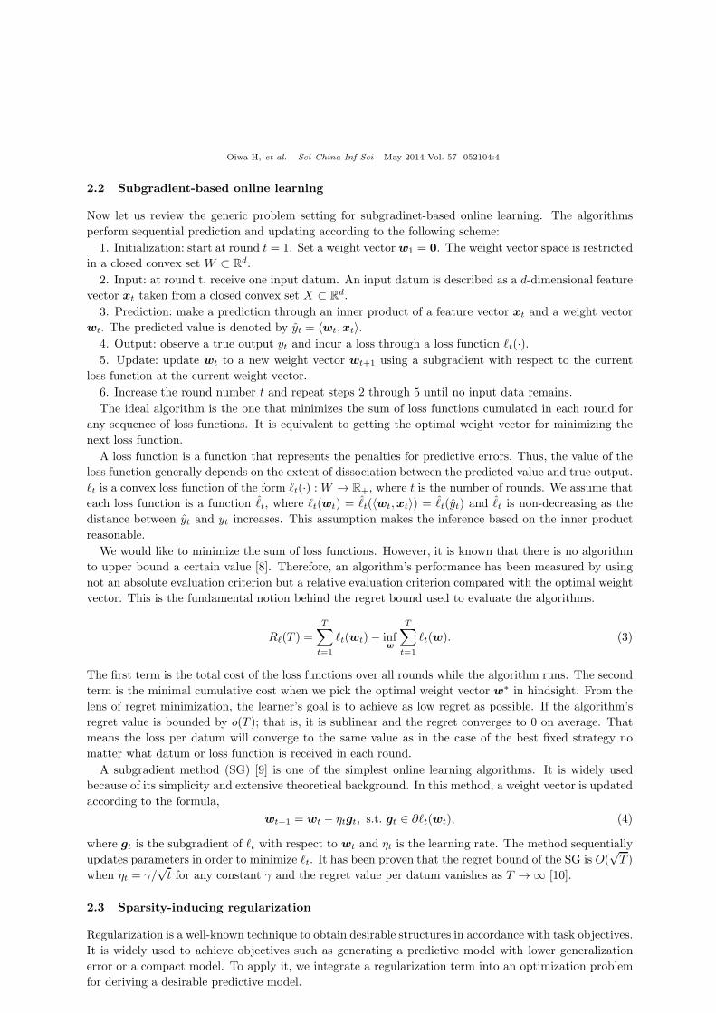
2.2 Subgradient-based online learning
Now let us review the generic problem setting for subgradinet-based online learning. The algorithms
perform sequential prediction and updating according to the following scheme:
1. Initialization: start at round t = 1. Set a weight vectorw1 = 0. The weight vector space is restricted
in a closed convex set W ⊂ Rd.
2. Input: at round t, receive one input datum. An input datum is described as a d-dimensional feature
vector xt taken from a closed convex set X ⊂ Rd.
3. Prediction: make a prediction through an inner product of a feature vector xt and a weight vector
wt. The predicted value is denoted by yt = 〈wt,xt〉.4. Output: observe a true output yt and incur a loss through a loss function �t(·).5. Update: update wt to a new weight vector wt+1 using a subgradient with respect to the current
loss function at the current weight vector.
6. Increase the round number t and repeat steps 2 through 5 until no input data remains.
The ideal algorithm is the one that minimizes the sum of loss functions cumulated in each round for
any sequence of loss functions. It is equivalent to getting the optimal weight vector for minimizing the
next loss function.
A loss function is a function that represents the penalties for predictive errors. Thus, the value of the
loss function generally depends on the extent of dissociation between the predicted value and true output.
�t is a convex loss function of the form �t(·) :W → R+, where t is the number of rounds. We assume that
each loss function is a function �t, where �t(wt) = �t(〈wt,xt〉) = �t(yt) and �t is non-decreasing as the
distance between yt and yt increases. This assumption makes the inference based on the inner product
reasonable.
We would like to minimize the sum of loss functions. However, it is known that there is no algorithm
to upper bound a certain value [8]. Therefore, an algorithm’s performance has been measured by using
not an absolute evaluation criterion but a relative evaluation criterion compared with the optimal weight
vector. This is the fundamental notion behind the regret bound used to evaluate the algorithms.
R�(T ) =
T∑
t=1
�t(wt)− infw
T∑
t=1
�t(w). (3)
The first term is the total cost of the loss functions over all rounds while the algorithm runs. The second
term is the minimal cumulative cost when we pick the optimal weight vector w∗ in hindsight. From the
lens of regret minimization, the learner’s goal is to achieve as low regret as possible. If the algorithm’s
regret value is bounded by o(T ); that is, it is sublinear and the regret converges to 0 on average. That
means the loss per datum will converge to the same value as in the case of the best fixed strategy no
matter what datum or loss function is received in each round.
A subgradient method (SG) [9] is one of the simplest online learning algorithms. It is widely used
because of its simplicity and extensive theoretical background. In this method, a weight vector is updated
according to the formula,
wt+1 = wt − ηtgt, s.t. gt ∈ ∂�t(wt), (4)
where gt is the subgradient of �t with respect to wt and ηt is the learning rate. The method sequentially
updates parameters in order to minimize �t. It has been proven that the regret bound of the SG is O(√T )
when ηt = γ/√t for any constant γ and the regret value per datum vanishes as T → ∞ [10].
2.3 Sparsity-inducing regularization
Regularization is a well-known technique to obtain desirable structures in accordance with task objectives.
It is widely used to achieve objectives such as generating a predictive model with lower generalization
error or a compact model. To apply it, we integrate a regularization term into an optimization problem
for deriving a desirable predictive model.
Oiwa H, et al. Sci China Inf Sci May 2014 Vol. 57 052104:5
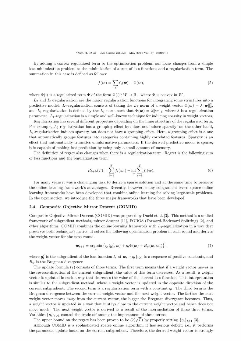
By adding a convex regularized term to the optimization problem, our focus changes from a simple
loss minimization problem to the minimization of a sum of loss functions and a regularization term. The
summation in this case is defined as follows:
f(w) =∑
t
�t(w) + Φ(w), (5)
where Φ(·) is a regularized term Φ of the form Φ(·) : W → R+ where Φ is convex in W .
L2 and L1-regularization are the major regularization functions for integrating some structures into a
predictive model. L2-regularization consists of taking the L2 norm of a weight vector Φ(w) = λ‖w‖22,and L1-regularization is defined by the L1 norm such that Φ(w) = λ‖w‖1, where λ is a regularization
parameter. L1-regularization is a simple and well-known technique for inducing sparsity in weight vectors.
Regularization has several different properties depending on the inner structure of the regularized term.
For example, L2-regularization has a grouping effect but does not induce sparsity; on the other hand,
L1-regularization induces sparsity but does not have a grouping effect. Here, a grouping effect is a one
that automatically groups features into categories containing highly correlated features. Sparsity is an
effect that automatically truncates uninformative parameters. If the derived predictive model is sparse,
it is capable of making fast prediction by using only a small amount of memory.
The definition of regret also changes when there is a regularization term. Regret is the following sum
of loss functions and the regularization term:
R�+Φ(T ) =
T∑
t=1
ft(wt)− infw
T∑
t=1
ft(w). (6)
For many years it was a challenging task to derive a sparse solution and at the same time to preserve
the online learning framework’s advantages. Recently, however, many subgradient-based sparse online
learning frameworks have been developed that combine online learning for solving large-scale problems.
In the next section, we introduce the three major frameworks that have been developed.
2.4 Composite Objective Mirror Descent (COMID)
Composite-Objective Mirror Descent (COMID) was proposed by Duchi et al. [3]. This method is a unified
framework of subgradient methods, mirror descent [11], FOBOS (Forward-Backward Splitting) [2], and
other algorithms. COMID combines the online learning framework with L1-regularization in a way that
preserves both technique’s merits. It solves the following optimization problem in each round and derives
the weight vector for the next round.
wt+1 = argminw
{ηt〈g�t ,w〉+ ηtΦ(w) +Bψ(w,wt)
}, (7)
where g�t is the subgradient of the loss function �t at wt, {ηt}t�1 is a sequence of positive constants, and
Bψ is the Bregman divergence.
The update formula (7) consists of three terms. The first term means that if a weight vector moves in
the reverse direction of the current subgradient, the value of this term decreases. As a result, a weight
vector is updated in such a way that decreases the value of the current loss function. This interpretation
is similar to the subgradient method, where a weight vector is updated in the opposite direction of the
current subgradient. The second term is a regularization term with a constant ηt. The third term is the
Bregman divergence between the current weight vector and the next weight vector. The farther the next
weight vector moves away from the current vector, the bigger the Bregman divergence becomes. Thus,
a weight vector is updated in a way that it stays close to the current weight vector and hence does not
move much. The next weight vector is derived as a result of the intermediation of these three terms.
Variables {ηt}t�1 control the trade-off among the importances of these terms.
The upper bound on the regret has been proven to be O(√T ) by properly setting {ηt}t�1 [3].
Although COMID is a sophisticated sparse online algorithm, it has serious deficit; i.e., it performs
the parameter update based on the current subgradient. Therefore, the derived weight vector is strongly
Oiwa H, et al. Sci China Inf Sci May 2014 Vol. 57 052104:6
influenced by the most recent data. For example, in the case of L1-regularization, COMID tends to
retain the parameters that have corresponding features which occur recently even if these features are
not crucial to the prediction.
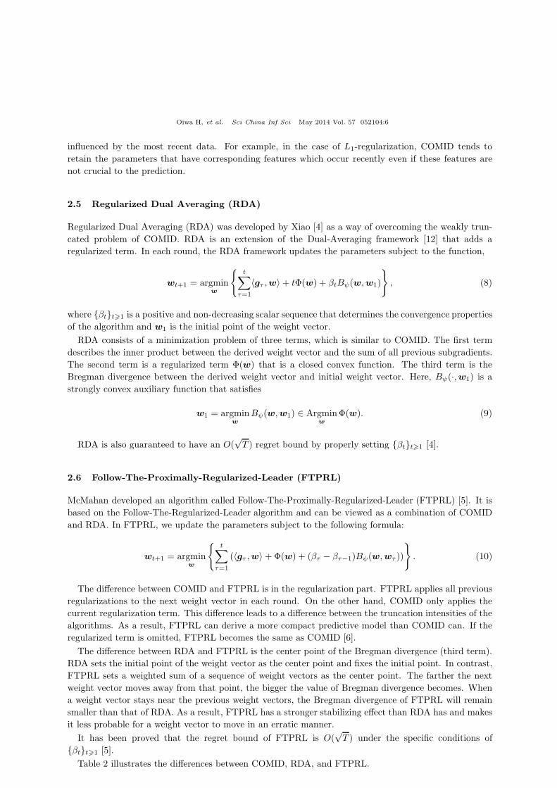
2.5 Regularized Dual Averaging (RDA)
Regularized Dual Averaging (RDA) was developed by Xiao [4] as a way of overcoming the weakly trun-
cated problem of COMID. RDA is an extension of the Dual-Averaging framework [12] that adds a
regularized term. In each round, the RDA framework updates the parameters subject to the function,
wt+1 = argminw
{t∑
τ=1
〈gτ ,w〉+ tΦ(w) + βtBψ(w,w1)
}, (8)
where {βt}t�1 is a positive and non-decreasing scalar sequence that determines the convergence properties
of the algorithm and w1 is the initial point of the weight vector.
RDA consists of a minimization problem of three terms, which is similar to COMID. The first term
describes the inner product between the derived weight vector and the sum of all previous subgradients.
The second term is a regularized term Φ(w) that is a closed convex function. The third term is the
Bregman divergence between the derived weight vector and initial weight vector. Here, Bψ(·,w1) is a
strongly convex auxiliary function that satisfies
w1 = argminw
Bψ(w,w1) ∈ Argminw
Φ(w). (9)
RDA is also guaranteed to have an O(√T ) regret bound by properly setting {βt}t�1 [4].
2.6 Follow-The-Proximally-Regularized-Leader (FTPRL)
McMahan developed an algorithm called Follow-The-Proximally-Regularized-Leader (FTPRL) [5]. It is
based on the Follow-The-Regularized-Leader algorithm and can be viewed as a combination of COMID
and RDA. In FTPRL, we update the parameters subject to the following formula:
wt+1 = argminw
{t∑
τ=1
(〈gτ ,w〉+Φ(w) + (βτ − βτ−1)Bψ(w,wτ ))
}. (10)
The difference between COMID and FTPRL is in the regularization part. FTPRL applies all previous
regularizations to the next weight vector in each round. On the other hand, COMID only applies the
current regularization term. This difference leads to a difference between the truncation intensities of the
algorithms. As a result, FTPRL can derive a more compact predictive model than COMID can. If the
regularized term is omitted, FTPRL becomes the same as COMID [6].
The difference between RDA and FTPRL is the center point of the Bregman divergence (third term).
RDA sets the initial point of the weight vector as the center point and fixes the initial point. In contrast,
FTPRL sets a weighted sum of a sequence of weight vectors as the center point. The farther the next
weight vector moves away from that point, the bigger the value of Bregman divergence becomes. When
a weight vector stays near the previous weight vectors, the Bregman divergence of FTPRL will remain
smaller than that of RDA. As a result, FTPRL has a stronger stabilizing effect than RDA has and makes
it less probable for a weight vector to move in an erratic manner.
It has been proved that the regret bound of FTPRL is O(√T ) under the specific conditions of
{βt}t�1 [5].
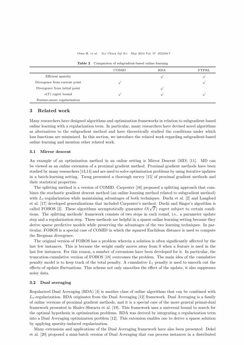
Table 2 illustrates the differences between COMID, RDA, and FTPRL.
Oiwa H, et al. Sci China Inf Sci May 2014 Vol. 57 052104:7
Table 2 Comparison of subgradient-based online learning
COMID RDA FTPRL
Efficient sparsity√ √
Divergence from current point√ √
Divergence from initial point√
o(T ) regret bound√ √ √
Feature-aware regularization
3 Related work
Many researchers have designed algorithms and optimization frameworks in relation to subgradient-based
online learning with a regularization term. In particular, many researchers have devised novel algorithms
as alternatives to the subgradient method and have theoretically studied the conditions under which
loss functions are minimized. In this section, we introduce the related work regarding subgradient-based
online learning and mention other related work.
3.1 Mirror descent
An example of an optimization method in an online setting is Mirror Descent (MD) [11]. MD can
be viewed as an online extension of a proximal gradient method. Proximal gradient methods have been
studied by many researchers [13,14] and are used to solve optimization problems by using iterative updates
in a batch-learning setting. Tseng presented a thorough survey [15] of proximal gradient methods and
their statistical properties.
The splitting method is a version of COMID. Carpenter [16] proposed a splitting approach that com-
bines the stochastic gradient descent method (an online learning method related to subgradient method)
with L1-regularization while maintaining advantages of both techniques. Duchi et al. [2] and Langford
et al. [17] developed generalizations that included Carpenter’s method. Duchi and Singer’s algorithm is
called FOBOS [2]. These algorithms asymptotically guarantee O(√T ) regret subject to certain condi-
tions. The splitting methods’ framework consists of two steps in each round, i.e., a parameter update
step and a regularization step. These methods are helpful in a sparse online learning setting because they
derive sparse predictive models while preserving the advantages of the two learning techniques. In par-
ticular, FOBOS is a special case of COMID in which the squared Euclidean distance is used to compute
the Bregman divergence.
The original version of FOBOS has a problem wherein a solution is often significantly affected by the
last few instances. This is because the weight easily moves away from 0 when a feature is used in the
last few instances. For this reason, a number of extensions have been developed for it. In particular, the
truncation-cumulative version of FOBOS [18] overcomes the problem. The main idea of the cumulative
penalty model is to keep track of the total penalty. A cumulative L1 penalty is used to smooth out the
effects of update fluctuations. This scheme not only smoothes the effect of the update, it also suppresses
noisy data.
3.2 Dual averaging
Regularized Dual Averaging (RDA) [4] is another class of online algorithms that can be combined with
L1-regularization. RDA originates from the Dual Averaging [12] framework. Dual Averaging is a family
of online versions of proximal gradient methods, and it is a special case of the more general primal-dual
framework presented in Shalev-Shwartz et al. [19]. This framework uses a universal bound to search for
the optimal hypothesis in optimization problems. RDA was derived by integrating a regularization term
into a Dual Averaging optimization problem [12]. This extension enables one to derive a sparse solution
by applying sparsity-induced regularization.
Many extensions and applications of the Dual Averaging framework have also been presented. Dekel
et al. [20] proposed a mini-batch version of Dual Averaging that can process instances in a distributed
Oiwa H, et al. Sci China Inf Sci May 2014 Vol. 57 052104:8
environment and proved an asymptotically optimal regret bound for smooth convex loss functions and
stochastic examples. Duchi et al. [21] derived a distributed algorithm based on the Dual Averaging
that works over a network. This algorithm does not have a central node and updates parameters by
using information from adjacent nodes. Distributed Dual Averaging has a theoretical regret bound that
is affected by the network structure. Lee et al. [22] showed that RDA is able to identify a manifold
in a weight space induced by a regularized term. This study led to the development of a new Dual
Averaging-based algorithm that works by identifying low-dimensional manifold structures. Duchi et
al. [23] proposed a parameter update scheme called AdaGrad. To emphasize rare features, AdaGrad
incorporates an appropriate Bregman divergence structure on-the-fly in the learning scheme. Thus,
AdaGrad has a similar intention to ours of emphasizing rare features, although it is different from our
framework. First, AdaGrad does not normalize the range of each feature’s value in an online setting.
Second, it does not reflect information on a just received datum because it controls the importance of a
feature by using only the Bregman divergence.
3.3 Regularized-follow-the-leader
The Follow-The-Leader algorithm (FTL) [24] and Regularized-Follow-The-Leader (RFTL) [25] were de-
veloped to make predictions with the help of expert advice and are ancestors of FTPRL. RFTL is a
combination of regularization and FTL. By adding a regularized term to FTL, we can prevent a weight
vector from moving wildly and thereby obtain a generalized solution and tighter regret bound. RFTL,
under some restrictions, also has an O(√T ) upper regret bound [25,26]. FTPRL is derived by inserting
Bregman divergences into RFTL. Previous studies [6] have shown the equivalence of RFTL and MD
as update procedures. They also have shown that FTPRL, COMID, and RDA are equivalent if their
Bregman divergences are properly set.
3.4 Other online learning algorithms and sparsity-inducing regularizations
A number of non-subgradient-based online algorithms have been developed for classification tasks. Most
of them set objectives such as minimizing the number of classification errors. The Perceptron [27], Passive-
Aggressive [28], and Confidence-Weighted [29,30] algorithms are well-known alternatives to subgradient-
based approaches. These algorithms are all guaranteed to bound the number of classification mistakes
to a constant value in the case of linearly separable. In particular, Confidence-Weighted algorithms form
a state-of-the-art framework for online classification tasks and significantly outperform other algorithms
with respect to their classification accuracy and convergence speed. Confidence-Weighted algorithms use
a Gaussian distributed weight vectors and update the parameters according to the covariances of the
weight vector in order to emphasize informative rare features. However, Confidence-Weighted algorithms
does not have any guarantee when it generates sparse solutions.
Narayanan et al. [31] proposed a new approach based on sampling from the time-varying Gibbs distri-
bution and connected online convex optimization and sampling from logconcave distribution on a convex
body. They derived a computationally efficient algorithm to solve the optimization problem in an online
manner. Cesa-Bianchi et al. [32] focused on binary classification and presented a new online algorithm
using randomized rounding of loss subgradients. This algorithm assigns labels to unlabeled data except
a received datum by randomized rounding, and then it computes and compares the empirical risk values
when it assigns each label to the remaining datum. Then, it decides the datum’s label dependence on
the difference between two values.
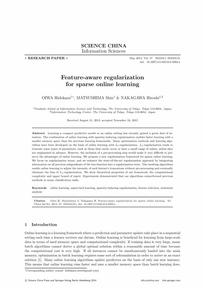
There are many regularization methods other than L1 and L2-regularization. Elastic net [33] is a
combination of L1-regularization and L2-regularization that has both sparsity and grouping effects. OS-
CAR [34] combines L1-regularization and pair-wise L∞-regularization. OSCAR has a strong grouping
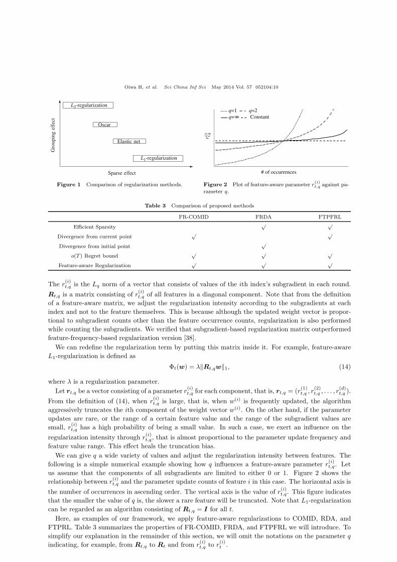
effect because the pair-wise L∞ norm pushes weights toward other weights near 0. Figure 1 compares
the properties of the different regularization methods. Furthermore, many sparsity-inducing methods are
used for feature learning [35,36] and subspace learning [37].
Oiwa H, et al. Sci China Inf Sci May 2014 Vol. 57 052104:9
4 Feature-aware regularization for sparse online learning
A large skewness exists among features in many tasks, including those of Natural Language Processing
and Pattern Recognition. However, subgradient-based sparse online algorithms like COMID, RDA, or
FTPRL do not take this bias into account. Therefore, learning using subgradient-based online algorithms
that includes the sparsity effect tends to truncate certain characteristic features even if they are crucial
for making a prediction. We show two examples in which plain L1-regularization causes problems in
sparse online learning.
4.1 Feature occurrence frequency problem
Suppose we want to use RDA with a simple L1-regularization. Let Φ(w) = λ‖w‖1, where λ is a positive
constant for controlling the intensity of regularization, and Bψ(w,w1) = ‖w − w1‖22/2 = ‖w‖22/2. In
addition, let us assume βt = 1/√t. In this case, we can derive a coordinate-wise update formula:
w(i)t+1 =
{0, if |g(i)t | � λ,
t√t(−g(i)t + sgn(g
(i)t )λ), otherwise,
(11)
where gt is the average value of the subgradients of the loss functions in the range from 1 to t. Let
us apply this simple RDA to a dataset in which the occurrence rate of feature A is 1/100 and that of
feature B is 1/2. Feature A inevitably becomes 0 unless the average absolute value of the Ath index
of the subgradients exceeds 100λ. That means it satisfies g(A) � 100λ, where g(i) is the average of the
ith absolute values of the subgradients by taking the ith index to be non-zero. On the other hand, the
weight of feature B is not always truncated to 0, wherein g(B) � 2λ. Therefore, if the feature occurrence
frequency is highly skewed, which happens in many tasks, the algorithm might fail to retain features that
are rare but helpful for making predictions. The same thing happens with COMID and FTPRL.
4.2 Value range problem
The disparity in the range of features affects the truncation, too. Let us assume a dataset with two
features : feature C and feature D. Feature C is an arbitrary feature, and feature D is a one whose value
is exactly 1000 times larger than that of feature C. Although they both have the same importance when
it comes to predictions, the weight of feature C is truncated faster than that of feature D when RDA is
learning from this dataset. That is, the following inequality is satisfied.
|g(C)| � λ � |g(D)|, (12)
where g(i) is the average of the ith indexes of all previous subgradients. We can easily see from formula (11)
that the weight of feature i is truncated if the ith index of the average subgradient is less than λ. Therefore,
when inequality (12) is satisfied, only feature C is truncated; feature D is not. The converse phenomenon
does not occur.
4.3 Feature-aware regularization for sparse online learning
To overcome these truncation problems, we designed a feature-aware regularization framework to retain
informative features in an online setting without pre-processing. Our framework integrates the weight
update information from all previous subgradients into a regularization term so as to adjust the intensity
of the truncation. In this framework, we define the feature-aware matrix
Rt,q =
⎛
⎜⎜⎜⎜⎜⎝
r(1)t,q 0 . . . 0
0 r(2)t,q . . . 0
......
. . ....
0 0 . . . r(d)t,q
⎞
⎟⎟⎟⎟⎟⎠, s.t. r
(i)t,q =
q
√∑t
τ=1
∣∣∣g(i)τ∣∣∣q
. (13)
Oiwa H, et al. Sci China Inf Sci May 2014 Vol. 57 052104:10
�
�
Sparse effect
Gro
upin
geff
ect
L1-regularization
Elastic net
Oscar
L2-regularization
Figure 1 Comparison of regularization methods.
r t,q(i)
q=1 q=2q=∞ Constant
# of occurrences
Figure 2 Plot of feature-aware parameter r(i)t,q against pa-
rameter q.
Table 3 Comparison of proposed methods
FR-COMID FRDA FTPFRL
Efficient Sparsity√ √
Divergence from current point√ √
Divergence from initial point√
o(T ) Regret bound√ √ √
Feature-aware Regularization√ √ √
The r(i)t,q is the Lq norm of a vector that consists of values of the ith index’s subgradient in each round.
Rt,q is a matrix consisting of r(i)t,q of all features in a diagonal component. Note that from the definition
of a feature-aware matrix, we adjust the regularization intensity according to the subgradients at each
index and not to the feature themselves. This is because although the updated weight vector is propor-
tional to subgradient counts other than the feature occurrence counts, regularization is also performed
while counting the subgradients. We verified that subgradient-based regularization matrix outperformed
feature-frequency-based regularization version [38].
We can redefine the regularization term by putting this matrix inside it. For example, feature-aware
L1-regularization is defined as
Φt(w) = λ‖Rt,qw‖1, (14)
where λ is a regularization parameter.
Let rt,q be a vector consisting of a parameter r(i)t,q for each component, that is, rt,q = (r
(1)t,q , r
(2)t,q , . . . , r
(d)t,q ).
From the definition of (14), when r(i)t,q is large, that is, when w(i) is frequently updated, the algorithm
aggressively truncates the ith component of the weight vector w(i). On the other hand, if the parameter
updates are rare, or the range of a certain feature value and the range of the subgradient values are
small, r(i)t,q has a high probability of being a small value. In such a case, we exert an influence on the
regularization intensity through r(i)t,q , that is almost proportional to the parameter update frequency and
feature value range. This effect heals the truncation bias.
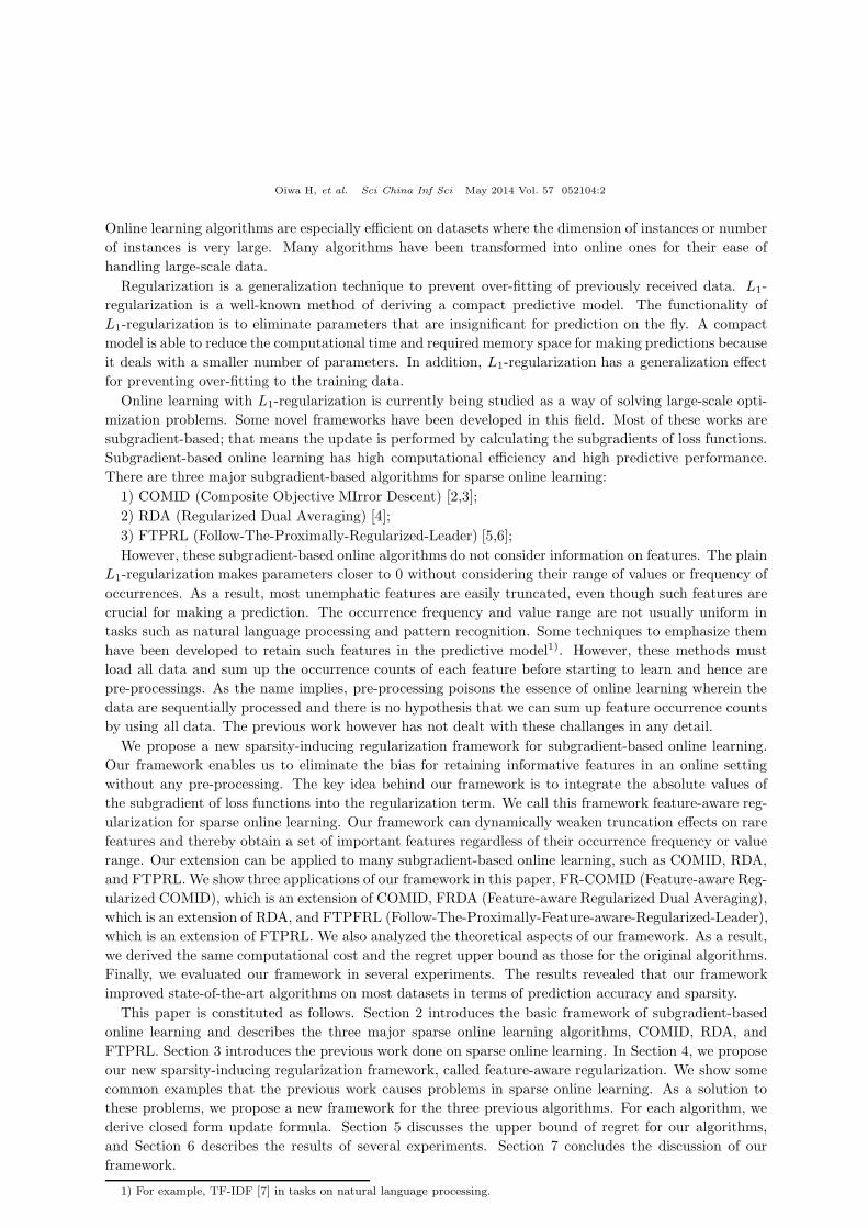
We can give q a wide variety of values and adjust the regularization intensity between features. The
following is a simple numerical example showing how q influences a feature-aware parameter r(i)t,q . Let
us assume that the components of all subgradients are limited to either 0 or 1. Figure 2 shows the
relationship between r(i)t,q and the parameter update counts of feature i in this case. The horizontal axis is
the number of occurrences in ascending order. The vertical axis is the value of r(i)t,q. This figure indicates
that the smaller the value of q is, the slower a rare feature will be truncated. Note that L1-regularization
can be regarded as an algorithm consisting of Rt,q = I for all t.
Here, as examples of our framework, we apply feature-aware regularizations to COMID, RDA, and
FTPRL. Table 3 summarizes the properties of FR-COMID, FRDA, and FTPFRL we will introduce. To
simplify our explanation in the remainder of this section, we will omit the notations on the parameter q
indicating, for example, from Rt,q to Rt and from r(i)t,q to r
(i)t .
Oiwa H, et al. Sci China Inf Sci May 2014 Vol. 57 052104:11
4.4 Feature-aware regularized COMID
Let us apply feature-aware regularization to COMID. We name this algorithm as Feature-aware Regu-
larized Composite Objective Mirror Descent (FR-COMID). The optimization problem can be written as
wt+1 = argminw
{ηt〈gt,w〉+ ηtΦt(w) +Bψ(w,wt)} . (15)
The difference between the original COMID (7) and FR-COMID is in the regularized term.
As a motivating example, let us derive a closed update formula in which Bψ(w,wt) = ‖w −wt‖22/2,and Φt(w) is the feature-aware L1-regularization defined in (14). While this formula is strongly convex
with respect to the weight vector, the coordinate-wise closed from is derived from the differential of it
with respect to the weight vector.
ηtg(i)t + ηtλr
(i)t ξ
(i)t + w
(i)t+1 − w
(i)t = 0, (16)
where ξ(i)t is the subgradient of |w(i)
t+1|. The value of ξ(i)t changes according to the value of w
(i)t+1. ξ
(i)t = 1
if w(i)t+1 > 0, ξ
(i)t = −1 if w
(i)t+1 < 0, or {ξ ∈ R| − 1 � ξ � 1} if w
(i)t+1 = 0.
As summarized (16), we can derive the update function as follows:
w(i)t+1 =
⎧⎨
⎩0, v
(i)t � 0,
sgn(w
(i)t − ηtg
(i)t
)v(i)t , otherwise,
(17)
where v(i)t =
∣∣∣w(i)t − ηtg
(i)t
∣∣∣− ηtλr(i)t .
From this update formula, we can see that r(i)t adjusts the intensity of the truncation so as to retain
informative but rarely occurring features. Formula (17) shows that FR-COMID with L1-regularization
can process one datum at O(d) computational cost. It is as fast as COMID.
The update procedure is summarized in Algorithm 1.
Algorithm 1 Feature-aware Regularized Composite Objective Mirror Descent (FR-COMID).
Require:
1: {ηt}t�1 is a positive nonincreasing sequence.
2: w1 = 0.
Algorithm:
1: for t = 1, 2, . . . do
2: Given a loss function �t, compute the subgradient gt ∈ ∂�t(wt) .
3: Derive a new weight vector wt+1:
w(i)t+1 =
⎧⎨
⎩
0, v(i)t � 0,
sign(w
(i)t − ηtg
(i)t
)v(i)t , otherwise,
(18)
where v(i)t =
∣∣∣w
(i)t − ηtg
(i)t
∣∣∣− ηtλr
(i)t .
4: end for
4.4.1 Lazy update
FR-COMID with L1-regularization allows us to truncate parameters in a lazy fashion [39]. We do not
need to apply regularization to the weights of features that do not occur in the current datum; thus, we
can postpone the regularization effect in each round. Such an updating scheme enables us to speed up
the process when the input vectors are very sparse and the dimension is very large.
We define the cumulative value of the total L1-regularization from τ = 1 to t as
ut = λt∑
τ=1
ητ . (19)
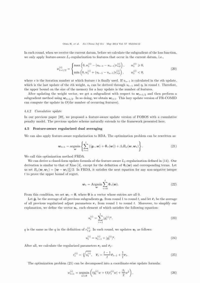
Oiwa H, et al. Sci China Inf Sci May 2014 Vol. 57 052104:12
In each round, when we receive the current datum, before we calculate the subgradient of the loss function,
we only apply feature-aware L1-regularization to features that occur in the current datum, i.e.,
w(i)t+1/2 =
⎧⎨
⎩max
(0, w
(i)t − (ut−1 − us−1)r
(i)s,p
), w
(i)t � 0,
min(0, w
(i)t + (ut−1 − us−1)r
(i)s,p
), w
(i)t < 0,
(20)
where s is the iteration number at which feature i is finally used. If us−1 is calculated in the sth update,
which is the last update of the ith weight, ut can be derived through ut−1 and ηt in round t. Therefore,
the upper bound on the size of the memory for a lazy update is the number of features.
After updating the weight vector, we get a subgradient with respect to wt+1/2 and then perform a
subgradient method using wt+1/2. In so doing, we obtain wt+1. This lazy update version of FR-COMID
can compute the update in O(the number of occurring features).
4.4.2 Cumulative update
In our previous paper [39], we proposed a feature-aware update version of FOBOS with a cumulative
penalty model. The previous update scheme naturally extends to the framework presented here.
4.5 Feature-aware regularized dual averaging
We can also apply feature-aware regularization to RDA. The optimization problem can be rewritten as:
wt+1 = argminw
{t∑
τ=1
(〈gτ ,w〉+Φτ (w)) + βtBψ(w,w1)
}. (21)
We call this optimization method FRDA.
We can derive a closed-form update formula of the feature-aware L1-regularization defined in (14). Our
derivation is similar to that of Xiao [4], except for the definition of Φt(w) and corresponding terms. Let
us set Bψ(w,w1) = ‖w −w1‖22/2. In FRDA, it satisfies the next equation for any non-negative integer
t to prove the upper bound of regret.
w1 = Argminw
t∑
τ=0
Φτ (w). (22)
From this condition, we set w1 = 0, where 0 is a vector whose entries are all 0.
Let gt be the average of all previous subgradients gτ from round 1 to round t, and let rt be the average
of all previous regularized adjust parameters rτ from round 1 to round t. Moreover, to simplify our
explanation, we define the vector ut, each element of which satisfies the following equation:
u(i)t =
t∑
τ=1
|g(i)τ |q. (23)
q is the same as the q in the definition of r(i)t,q . In each round, we updates ut as follows:
u(i)t = u
(i)t−1 + |g(i)t |q. (24)
After all, we calculate the regularized parameters rt and rt:
r(i)t =
q
√u(i)t , rt =
t− 1
trt−1 +
1
trt. (25)
The optimization problem (21) can be decomposed into a coordinate-wise update formula:
w(i)t+1 = argmin
w∈R
(tg
(i)t w + tλ|r(i)t w|+ βt
2w2
). (26)
Oiwa H, et al. Sci China Inf Sci May 2014 Vol. 57 052104:13
From the definition of r(i)t , we clearly have r
(i)t � 0. Thus, the optimal solution to formula (26) is
subject to
g(i)t + λr
(i)t ξ(i) +
βttw
(i)t+1 = 0, (27)
where ξ(i) is the subgradient of |w(i)t+1|. The value of ξ
(i)t changes according to the value of w
(i)t+1. ξ
(i)t = 1
if w(i)t+1 > 0, ξ
(i)t = −1 if w
(i)t+1 < 0, or {ξ ∈ R| − 1 � ξ � 1} if w
(i)t+1 = 0.
Therefore, we can solve the optimization problem as follows:
1) If |g(i)t | � λr(i)t , set w
(i)t+1 = 0 and ξ(i) = −g(i)t /λr
(i)t . When w
(i)t+1 �= 0, Eq. (27) cannot be satisfied.
2) If g(i)t > λr
(i)t > 0, set w
(i)t+1 < 0 and ξ(i) = −1.
3) If g(i)t < −λr(i)t < 0, set w
(i)t+1 > 0 and ξ(i) = 1.
The above solution is summarized as
w(i)t+1 =
⎧⎪⎨
⎪⎩
0, v(i)t � 0,
−sign(g(i)t
) tv(i)tβt
, otherwise,(28)
where we have defined v(i)t =
∣∣∣g(i)t∣∣∣− λr
(i)t .
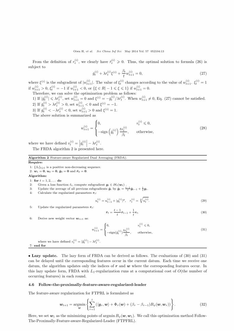
The FRDA algorithm 2 is presented here.
Algorithm 2 Feature-aware Regularized Dual Averaging (FRDA).
Require:
1: {βt}t�1 is a positive non-decreasing sequence.
2: w1 = 0, u0 = 0, g0 = 0 and r0 = 0.
Algorithm:
1: for t = 1, 2, . . . do
2: Given a loss function �t, compute subgradient gt ∈ ∂�t(wt) .
3: Update the average of all previous subgradients gt by gt =t−1t
gt−1 + 1tgt.
4: Calculate the regularized parameters rt:
u(i)t = u
(i)t−1 + |g(i)t |p, r
(i)t =
p√
u(i)t . (29)
5: Update the regularized parameters rt:
rt =t− 1
trt−1 +
1
trt. (30)
6: Derive new weight vector wt+1 as:
w(i)t+1 =
⎧⎪⎨
⎪⎩
0, v(i)t � 0,
−sign(g(i)t )
tv(i)t
βt, otherwise,
(31)
where we have defined v(i)t = |g(i)t | − λr
(i)t .
7: end for
• Lazy update. The lazy form of FRDA can be derived as follows. The evaluations of (30) and (31)
can be delayed until the corresponding features occur in the current datum. Each time we receive one
datum, the algorithm updates only the indices of r and w where the corresponding features occur. In
this lazy update form, FRDA with L1-regularization runs at a computational cost of O(the number of
occurring features) in each round.
4.6 Follow-the-proximally-feature-aware-regularized-leader
The feature-aware regularization for FTPRL is formulated as
wt+1 = argminw
{t∑
τ=1
(〈gτ ,w〉+Φτ (w) + (βτ − βτ−1)Bψ(w,wτ ))
}. (32)
Here, we set w1 as the minimizing points of argminBψ(w,w1). We call this optimization method Follow-
The-Proximally-Feature-aware-Regularized-Leader (FTPFRL).
Oiwa H, et al. Sci China Inf Sci May 2014 Vol. 57 052104:14
We will give a closed update formula for FTPFRL, where Bψ(w,wt) = ‖w −wt‖22/2, and Φτ (w) is
the feature-aware regularization (14). Let us assume that w1 is a zero vector and β0 = 0. The derivation
of the closed-form solution is similar to the one for FRDA. Thus, we will skip defining the variables g,
u, and r.
To simplify the following discussion, we define βt − βt−1 as βt. First, we summarize the sum of the
squared Euclidean norms as follows:
t∑
τ=1
βτ2‖w −wτ‖22 =
1
2
(t∑
τ=1
βτ‖w‖22 − 2βτwwτ + βτ‖wτ‖22)
=
∑βτ2
∥∥∥∥∥w −∑βτwτ∑βτ
∥∥∥∥∥
2
2
+ const =βt2
∥∥∥∥∥w − wβt
βt
∥∥∥∥∥
2
2
+ const, (33)
where∑βτ = βt from the definition of βτ and wβ
t =∑βτwτ . The constant term does not affect the
derivation of the next weight vector; therefore, we can ignore it.
Next, we calculate a new weight vectorwt+1. First, we derive rt by using (24), (25). Next, we introduce
a beta-weighted vector wβt wβ
t = wβt−1 + βtwt Since the optimization problem can be decomposed into
a coordinate-wise update formula and is a convex function with respect to w, we find that
g(i)t + λr
(i)t ξ(i) +
βtt
(w
(i)t+1 −
wβ,(i)t
βt
)= 0. (34)
As in the case of FRDA, the update formula is derived by properly assigning the value of ξ. The following
is a summary of the above solution:
w(i)t+1 =
⎧⎪⎨
⎪⎩
0, v(i)t � 0,
sgn(wβ,(i)t − tg
(i)t
) v(i)tβt
, otherwise,(35)
where we have defined v(i)t = |wβ,(i)t − tg
(i)t | − tλr
(i)t .
The FTPFRL algorithm 3 is listed below.
4.7 How to eliminate the truncation bias
Here, we illustrate how feature-aware regularization overcomes the rare feature truncation problem and
the value range problem.
Let us apply FRDA with L1-regularization to the example datasets described in Subsections 4.1 and
4.2. First, let us consider the dataset described in Subsection 4.1 under the condition that the parameter
settings are the same as RDA’s. As described before, RDA truncates feature A on a priority basis.
However, FRDA does not truncate feature A g(A) � 100λr(A)t , and furthermore, it does not truncate
feature B when g(B) � 2λr(B)t . From the definition of r
(i)t , while the occurrence frequency of feature B
is fifty times greater than that of feature A, it is expected that the value of r(B)t will be q
√50 larger than
the value of r(A)t when the importance of these features are similar. Thus, the intensity of truncation can
be adjusted so as to retain rare features.
Next, let us consider the value range problem. We assume that feature C and feature D in the dataset
have the same importance. However, in RDA, feature C would be truncated in an earlier round than
feature D. However, in FRDA, r(C)t is exactly 1000 times larger than r
(D)t in all rounds; thus, the value
of r(C)t is also exactly 1000 times larger than the value of r
(D)t . Therefore, if |g(C)
t | < λr(C)t , i.e., w
(C)t+1 = 0
is satisfied, |g(D)t | < λr
(D)t , i.e., w
(D)t = 0 is also satisfied. The converse is also true. Accordingly, even
if the range of feature values is skewed, FRDA automatically absorbs the disparity in the features and
adjusts the truncation intensity by using the parameter r.
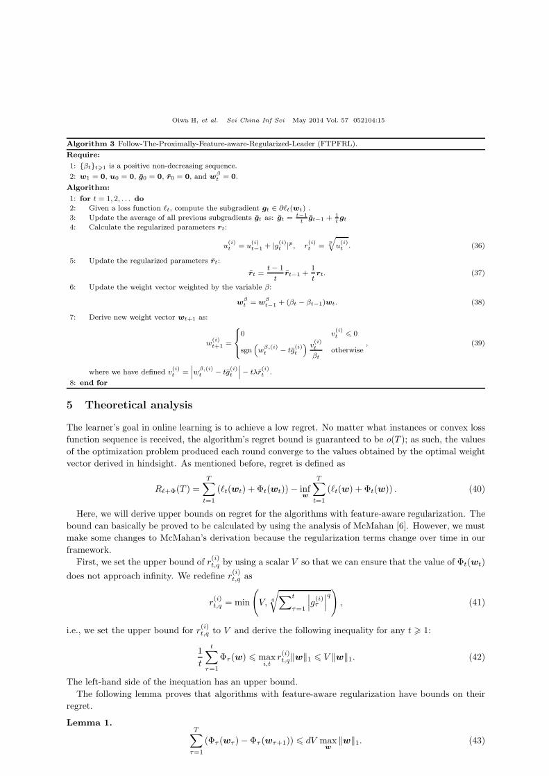
Oiwa H, et al. Sci China Inf Sci May 2014 Vol. 57 052104:15
Algorithm 3 Follow-The-Proximally-Feature-aware-Regularized-Leader (FTPFRL).
Require:
1: {βt}t�1 is a positive non-decreasing sequence.
2: w1 = 0, u0 = 0, g0 = 0, r0 = 0, and wβt = 0.
Algorithm:
1: for t = 1, 2, . . . do
2: Given a loss function �t, compute the subgradient gt ∈ ∂�t(wt) .
3: Update the average of all previous subgradients gt as: gt =t−1t
gt−1 + 1tgt
4: Calculate the regularized parameters rt:
u(i)t = u
(i)t−1 + |g(i)t |p, r
(i)t =
p√
u(i)t . (36)
5: Update the regularized parameters rt:
rt =t− 1
trt−1 +
1
trt. (37)
6: Update the weight vector weighted by the variable β:
wβt = wβ
t−1 + (βt − βt−1)wt. (38)
7: Derive new weight vector wt+1 as:
w(i)t+1 =
⎧⎪⎨
⎪⎩
0 v(i)t � 0
sgn(wβ,(i)t − tg
(i)t
) v(i)t
βtotherwise
, (39)
where we have defined v(i)t =
∣∣∣wβ,(i)t − tg
(i)t
∣∣∣− tλr
(i)t .
8: end for
5 Theoretical analysis
The learner’s goal in online learning is to achieve a low regret. No matter what instances or convex loss
function sequence is received, the algorithm’s regret bound is guaranteed to be o(T ); as such, the values
of the optimization problem produced each round converge to the values obtained by the optimal weight
vector derived in hindsight. As mentioned before, regret is defined as
R�+Φ(T ) =T∑
t=1
(�t(wt) + Φt(wt))− infw
T∑
t=1
(�t(w) + Φt(w)) . (40)
Here, we will derive upper bounds on regret for the algorithms with feature-aware regularization. The
bound can basically be proved to be calculated by using the analysis of McMahan [6]. However, we must
make some changes to McMahan’s derivation because the regularization terms change over time in our
framework.
First, we set the upper bound of r(i)t,q by using a scalar V so that we can ensure that the value of Φt(wt)
does not approach infinity. We redefine r(i)t,q as
r(i)t,q = min
(V, q
√∑t
τ=1
∣∣∣g(i)τ∣∣∣q), (41)
i.e., we set the upper bound for r(i)t,q to V and derive the following inequality for any t � 1:
1
t
t∑
τ=1
Φτ (w) � maxi,t
r(i)t,q‖w‖1 � V ‖w‖1. (42)
The left-hand side of the inequation has an upper bound.
The following lemma proves that algorithms with feature-aware regularization have bounds on their
regret.
Lemma 1.T∑
τ=1
(Φτ (wτ )− Φτ (wτ+1)) � dV maxw
‖w‖1. (43)
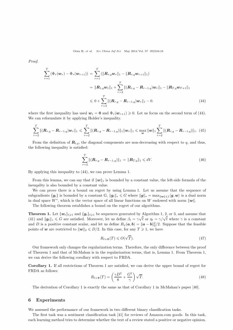
Oiwa H, et al. Sci China Inf Sci May 2014 Vol. 57 052104:16
Proof.
T∑
τ=1
(Φτ (wτ )− Φτ (wτ+1)) =
T∑
τ=1
(‖Rτ,qwτ‖1 − ‖Rτ,qwτ+1‖1)
= ‖R1,qw1‖1 +T∑
τ=2
‖(Rτ,q −Rτ−1,q)wτ‖1 − ‖RT,qwT+1‖1
� 0 +
T∑
τ=2
‖(Rτ,q −Rτ−1,q)wτ‖1 − 0. (44)
where the first inequality has used w1 = 0 and Φτ (wτ+1) � 0. Let us focus on the second term of (44).
We can reformulate it by applying Holder’s inequality.
T∑
τ=2
‖(Rτ,q −Rτ−1,q)wτ‖1 �T∑
τ=2
‖(Rτ,q −Rτ−1,q)‖1‖wτ‖1 � maxw
‖w‖1T∑
τ=2
‖(Rτ,q −Rτ−1,q)‖1. (45)
From the definition of Rt,q, the diagonal components are non-decreasing with respect to q, and thus,
the following inequality is satisfied:
T∑
τ=2
‖(Rτ,q −Rτ−1,q)‖1 = ‖RT,q‖1 � dV. (46)
By applying this inequality to (44), we can prove Lemma 1.
From this lemma, we can say that if ‖w‖1 is bounded by a constant value, the left-side formula of the
ineuqality is also bounded by a constant value.
We can prove there is a bound on regret by using Lemma 1. Let us assume that the sequence of
subgradients {gt} is bounded by a constant G, ‖gt‖∗ � G where ‖g‖∗ = max‖w‖�1〈g,w〉 is a dual norm
in dual space W ∗, which is the vector space of all linear functions on W endowed with norm ‖w‖.The following theorem establishes a bound on the regret of our algorithms.
Theorem 1. Let {wt}t�1 and {gt}t�1 be sequences generated by Algorithm 1, 2, or 3, and assume that
(41) and ‖gt‖∗ � G are satisfied. Moreover, let us define βt = γ√t or ηt = γ/
√t where γ is a constant
and D is a positive constant scalar, and let us define Bψ(a, b) = ‖a − b‖22/2. Suppose that the feasible
points of w are restricted to ‖w‖2 � D/2. In this case, for any T � 1, we have
R�+Φ(T ) � O(√T ). (47)
Our framework only changes the regularization terms. Therefore, the only difference between the proof
of Theorem 1 and that of McMahan is in the regularization terms, that is, Lemma 1. From Theorem 1,
we can derive the following corollary with respect to FRDA.
Corollary 1. If all restrictions of Theorem 1 are satisfied, we can derive the upper bound of regret for
FRDA as follows:
R�+Φ(T ) =
(γD2
8+G2
γ
)√T . (48)
The derivation of Corollary 1 is exactly the same as that of Corollary 1 in McMahan’s paper [40].
6 Experiments
We assessed the performance of our framework in two different binary classification tasks.
The first task was a sentiment classification task [41] for reviews of Amazon.com goods. In this task,
each learning method tries to determine whether the text of a review stated a positive or negative opinion.
Oiwa H, et al. Sci China Inf Sci May 2014 Vol. 57 052104:17
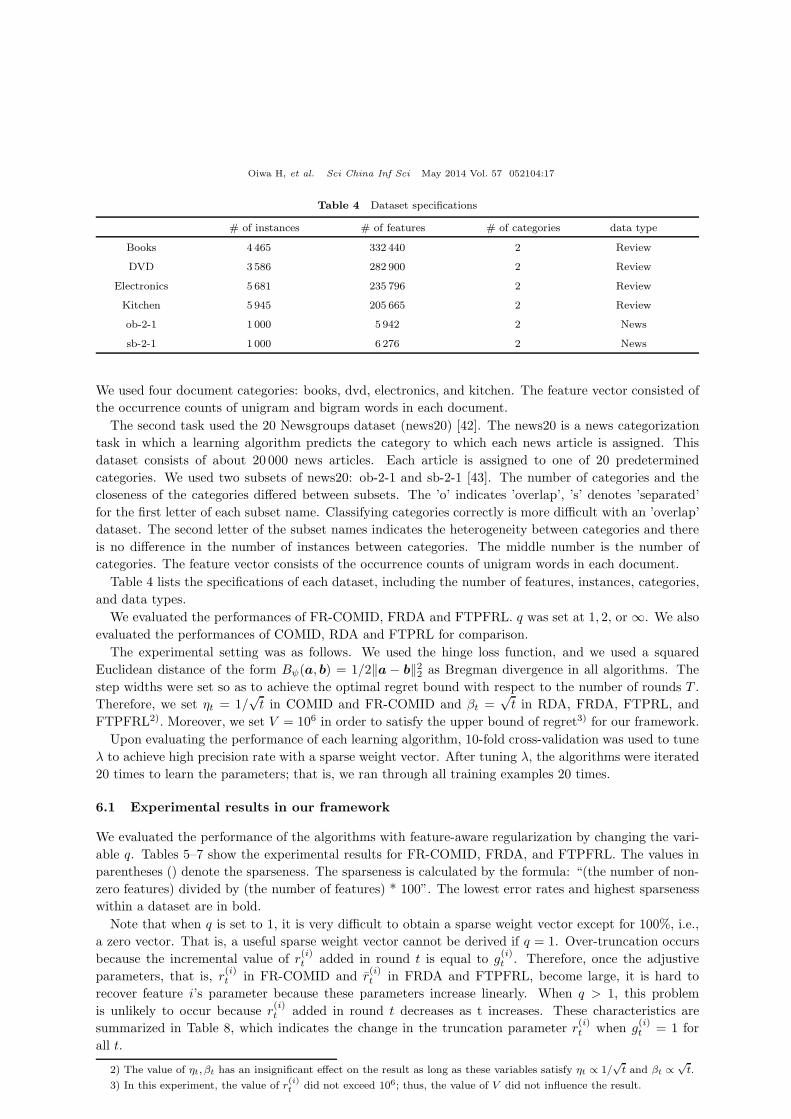
Table 4 Dataset specifications
# of instances # of features # of categories data type
Books 4 465 332 440 2 Review
DVD 3586 282 900 2 Review
Electronics 5 681 235 796 2 Review
Kitchen 5 945 205 665 2 Review
ob-2-1 1 000 5 942 2 News
sb-2-1 1 000 6 276 2 News
We used four document categories: books, dvd, electronics, and kitchen. The feature vector consisted of
the occurrence counts of unigram and bigram words in each document.
The second task used the 20 Newsgroups dataset (news20) [42]. The news20 is a news categorization
task in which a learning algorithm predicts the category to which each news article is assigned. This
dataset consists of about 20 000 news articles. Each article is assigned to one of 20 predetermined
categories. We used two subsets of news20: ob-2-1 and sb-2-1 [43]. The number of categories and the
closeness of the categories differed between subsets. The ’o’ indicates ’overlap’, ’s’ denotes ’separated’
for the first letter of each subset name. Classifying categories correctly is more difficult with an ’overlap’
dataset. The second letter of the subset names indicates the heterogeneity between categories and there
is no difference in the number of instances between categories. The middle number is the number of
categories. The feature vector consists of the occurrence counts of unigram words in each document.
Table 4 lists the specifications of each dataset, including the number of features, instances, categories,
and data types.
We evaluated the performances of FR-COMID, FRDA and FTPFRL. q was set at 1, 2, or ∞. We also
evaluated the performances of COMID, RDA and FTPRL for comparison.
The experimental setting was as follows. We used the hinge loss function, and we used a squared
Euclidean distance of the form Bψ(a, b) = 1/2‖a − b‖22 as Bregman divergence in all algorithms. The
step widths were set so as to achieve the optimal regret bound with respect to the number of rounds T .
Therefore, we set ηt = 1/√t in COMID and FR-COMID and βt =
√t in RDA, FRDA, FTPRL, and
FTPFRL2). Moreover, we set V = 106 in order to satisfy the upper bound of regret3) for our framework.
Upon evaluating the performance of each learning algorithm, 10-fold cross-validation was used to tune
λ to achieve high precision rate with a sparse weight vector. After tuning λ, the algorithms were iterated
20 times to learn the parameters; that is, we ran through all training examples 20 times.
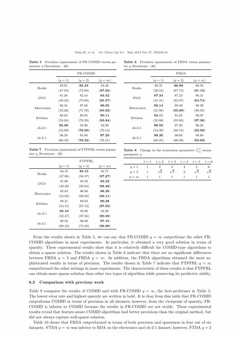
6.1 Experimental results in our framework
We evaluated the performance of the algorithms with feature-aware regularization by changing the vari-
able q. Tables 5–7 show the experimental results for FR-COMID, FRDA, and FTPFRL. The values in
parentheses () denote the sparseness. The sparseness is calculated by the formula: “(the number of non-
zero features) divided by (the number of features) * 100”. The lowest error rates and highest sparseness
within a dataset are in bold.
Note that when q is set to 1, it is very difficult to obtain a sparse weight vector except for 100%, i.e.,
a zero vector. That is, a useful sparse weight vector cannot be derived if q = 1. Over-truncation occurs
because the incremental value of r(i)t added in round t is equal to g
(i)t . Therefore, once the adjustive
parameters, that is, r(i)t in FR-COMID and r
(i)t in FRDA and FTPFRL, become large, it is hard to
recover feature i’s parameter because these parameters increase linearly. When q > 1, this problem
is unlikely to occur because r(i)t added in round t decreases as t increases. These characteristics are
summarized in Table 8, which indicates the change in the truncation parameter r(i)t when g
(i)t = 1 for
all t.
2) The value of ηt, βt has an insignificant effect on the result as long as these variables satisfy ηt ∝ 1/√t and βt ∝
√t.
3) In this experiment, the value of r(i)t did not exceed 106; thus, the value of V did not influence the result.
Oiwa H, et al. Sci China Inf Sci May 2014 Vol. 57 052104:18
Table 5 Precision (sparseness) of FR-COMID versus pa-
rameter q (Iterations : 20)
FR-COMID
(q = 1) (q = 2) (q = ∞)
Books83.91 85.24 84.46
(47.04) (72.69) (87.05)
DVD81.26 82.10 83.52
(49.43) (73.69) (85.57)
Electronics86.24 87.68 88.05
(53.26) (71.76) (85.62)
Kitchen88.63 88.95 90.11
(53.04) (78.29) (83.84)
ob-2-195.00 93.90 94.90
(52.89) (76.00) (70.14)
sb-2-196.50 95.80 97.20
(66.33) (78.32) (78.31)
Table 6 Precision (sparseness) of FRDA versus parame-
ter q (Iterations : 20)
FRDA
(q = 1) (q = 2) (q = ∞)
Books86.35 86.88 86.50
(30.34) (87.73) (91.13)
DVD87.34 87.23 86.31
(31.31) (82.97) (94.74)
Electronics90.14 89.49 89.30
(31.98) (95.89) (88.93)
Kitchen92.11 91.02 90.95
(35.08) (95.90) (97.36)
ob-2-198.50 97.20 96.20
(54.39) (80.74) (82.30)
sb-2-199.20 98.60 98.80
(60.25) (86.99) (93.69)
Table 7 Precision (sparseness) of FTPFRL versus param-
eter q (Iterations : 20)
FTPFRL
(q = 1) (q = 2) (q = ∞)
Books84.10 85.15 84.71
(47.90) (94.37) (97.27)
DVD81.06 83.29 83.32
(49.48) (90.94) (98.46)
Electronics85.83 86.80 88.29
(53.93) (96.93) (99.11)
Kitchen88.41 89.03 90.28
(54.15) (97.12) (97.50)
ob-2-195.10 93.90 94.90
(52.47) (87.56) (90.50)
sb-2-196.50 96.00 97.10
(68.10) (74.56) (96.98)
Table 8 Change in the truncation parameter r(i)t,q versus
parameter q
t = 1 t = 2 t = 3 t = 4 t = 5 t = 6
q = 1 1 2 3 4 5 6
q = 2 1√2
√3 2
√5
√6
q = ∞ 1 1 1 1 1 1
From the results shown in Table 5, we can say that FR-COMID q = ∞ outperforms the other FR-
COMID algorithms in most experiments. In particular, it obtained a very good solution in terms of
sparsity. These experimental results show that it is relatively difficult for COMID-type algorithms to
obtain a sparse solution. The results shown in Table 6 indicate that there are no significant differences
between FRDA q = 2 and FRDA q = ∞. In addition, the FRDA algorithms obtained the most so-
phisticated results in terms of precision. The results shown in Table 7 indicate that FTPFRL q = ∞outperformed the other settings in most experiments. The characteristic of these results is that FTPFRL
can obtain more sparse solution than other two types of algorithm while preserving its predictive ability.
6.2 Comparison with previous work
Table 9 compares the results of COMID and with FR-COMID q = ∞, the best-performer in Table 5.
The lowest error rate and highest sparsity are written in bold. It is clear from this table that FR-COMID
outperforms COMID in terms of precision in all datasets; however, from the viewpoint of sparsity, FR-
COMID is inferior to COMID because the results in FR-COMID are not stable. These experimental
results reveal that feature-aware COMID algorithms had better precisions than the original method, but
did not always capture well-sparse solution.
Table 10 shows that FRDA outperformed in terms of both precision and sparseness in four out of six
datasets. FTDA q = ∞ was inferior to RDA on the electronics and ob-2-1 dataset; however, FTDA q = 2
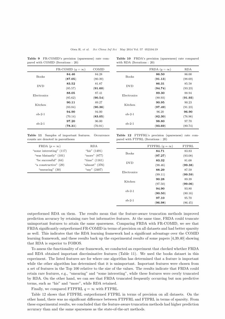
Oiwa H, et al. Sci China Inf Sci May 2014 Vol. 57 052104:19
Table 9 FR-COMID’s precision (sparseness) rate com-
pared with COMID (Iterations : 20)
FR-COMID (q = ∞) COMID
Books84.46 84.28
(87.05) (80.39)
DVD83.52 81.87
(85.57) (91.60)
Electronics88.05 87.41
(85.62) (90.54)
Kitchen90.11 89.27
(83.84) (90.36)
ob-2-194.90 94.00
(70.14) (83.05)
sb-2-197.20 96.00
(78.31) (70.91)
Table 10 FRDA’s precision (sparseness) rate compared
with RDA (Iterations : 20)
FRDA (q = ∞) RDA
Books86.50 86.00
(91.13) (88.69)
DVD86.31 85.58
(94.74) (93.23)
Electronics89.30 88.94
(88.93) (91.93)
Kitchen90.95 90.23
(97.49) (91.23)
ob-2-196.20 96.90
(82.30) (76.96)
sb-2-198.80 97.70
(93.69) (89.74)
Table 11 Samples of important features. Occurrence
counts are denoted in parentheses
FRDA (p = ∞) RDA
“some interesting” (117) “his” (1491)
“was blatantly” (101) “more” (877)
“be successful” (64) “time” (1161)
“a constructive” (29) “almost” (376)
“smearing” (30) “say” (2407)
Table 12 FTPFRL’s precision (sparseness) rate com-
pared with FTPRL (Iterations : 20)
FTPFRL (q = ∞) FTPRL
Books84.71 83.83
(97.27) (93.08)
DVD83.32 81.68
(98.46) (99.38)
Electronics88.29 87.59
(99.11) (99.59)
Kitchen90.28 89.39
(97.50) (99.06)
ob-2-194.90 93.80
(90.50) (80.16)
sb-2-197.10 95.70
(96.98) (86.45)
outperformed RDA on them. The results mean that the feature-aware truncation methods improved
prediction accuracy by retaining rare but informative features. At the same time, FRDA could truncate
unimportant features to attain the same sparseness. Comparing FRDA with FR-COMID, we see that
FRDA significantly outperformed FR-COMID in terms of precision on all datasets and had better sparsity
as well. This indicates that the RDA learning framework had a significant advantage over the COMID
learning framework, and these results back up the experimental results of some papers [4,39,40] showing
that RDA is superior to FOBOS.
To assess the functionality of our framework, we conducted an experiment that checked whether FRDA
and RDA obtained important discriminative features (Table 11). We used the books dataset in this
experiment. The listed features are for where one algorithm has determined that a feature is important
while the other algorithm has determined that it is unimportant. Important features were chosen from
a set of features in the Top 100 relative to the size of the values. The results indicate that FRDA could
retain rare features, e.g., “smearing” and “some interesting”, while these features were overly truncated
by RDA. On the other hand, we can see that FRDA truncated frequently occurring but non predictive
terms, such as “his” and “more”, while RDA retained.
Finally, we compared FTPFRL q = ∞ with FTPRL.
Table 12 shows that FTPFRL outperformed FTPRL in terms of precision on all datasets. On the
other hand, there was no significant difference between FTPFRL and FTPRL in terms of sparsity. From
these experimental results, we concluded that the feature-aware truncation methods had higher prediction
accuracy than and the same sparseness as the state-of-the-art methods.
Oiwa H, et al. Sci China Inf Sci May 2014 Vol. 57 052104:20
7 Conclusion
We proposed feature-aware regularization framework for sparse online learning to eliminate the truncation
biases. We proved theoretical guarantees of our framework by obtaining an upper bound on regret and
showed the computational efficiency of each algorithm. Experimental results revealed that our framework
outperformed the previous methods in terms of predictive ability, while preserving similar sparsity rates,
and that it retained rare but informative features.
One remaining issue is whether we can modify the algorithm to choose the optimal parameter q in an
online setting. We will investigate this question and further extend our proposed methods.
Acknowledgements
This work was supported by JSPS KAKENHI, Grant-in-Aid for JSPS Fellows for Hidekazu Oiwa.
References
1 Yu H-F, Hsieh C-J, Chang K-W, et al. Large linear classification when data cannot fit in memory. In: Proceedings of
the 16th ACM SIGKDD international conference on Knowledge discovery and data mining. New York: ACM, 2010.
833–842
2 Duchi J, Singer Y. Effcient online and batch learning using forward backward splitting. J Mach Learn Res, 2009, 10:
2899–2934
3 Duchi J, Shalev-Shwartz S, Singer Y, et al. Composite objective mirror descent. In: 23rd International Conference on
Learning Theory, Haifa, 2010. 14–26
4 Xiao L. Dual averaging methods for regularized stochastic learning and online optimization. J Mach Learn Res, 2010,
11: 2543–2596
5 Brendan McMahan H, Streeter M J. Adaptive bound optimization for online convex optimization. In: 23rd Interna-
tional Conference on Learning Theory, Haifa, 2010. 244–256
6 Brendan McMahan H. Follow-the-regularized-leader and mirror descent: equivalence theorems and l1 regularization.
In: 14th International Conference on Artificial Intelligence and Statistics, Ft. Lauderdale, 2011. 525–533
7 Salton G, Buckley C. Term-weighting approaches in automatic text retrieval. Inf Process Manage, 1988, 24: 513–523
8 Shalev-Shwartz S. Online learning and online convex optimization. Found Trends Mach Learn, 2012, 4: 107–194
9 Bertsekas D P. Nonlinear Programming. 2nd edition. Athena Scientific. 1999
10 Zinkevich M. Online convex programming and generalized infinitesimal gradient ascent. In: 20th International Con-
ference on Machine Learning, Washington D. C., 2003. 928–936
11 Beck A, Teboulle M. Mirror descent and nonlinear projected subgradient methods for convex optimization. Oper Res
Lett, 2003, 31: 167–175
12 Nesterov Y. Primal-dual subgradient methods for convex problems. Math Program, 2009, 120: 221–259
13 Nesterov Y. A method of solving a convex programming problem with convergence rate o(1/k2). Sov Math Dokl, 1983,
27: 372–376
14 Beck A, Teboulle M. A fast iterative shrinkage-thresholding algorithm for linear inverse problems. SIAM J Imag Sci,
2009, 2: 183–202
15 Tseng P. Approximation accuracy, gradient methods, and error bound for structured convex optimization. Math
Program, 2010, 125: 263–295
16 Carpenter B. Lazy sparse stochastic gradient descent for regularized multinomial logistic regression. Technical Report,
Alias-i, Inc. 2008
17 Langford J, Li L H, Zhang T. Sparse online learning via truncated gradient. J Mach Learn Res, 2009, 10: 777–801
18 Tsuruoka Y, Tsujii J, Ananiadou S. Stochastic gradient descent training for l1-regularized log-linear. In: Proceedings
of the Joint Conference of the 47th Annual Meeting of the ACL and the 4th International Joint Conference on Natural
Language Processing of the AFNLP. Stroudsburg: Association for Computational Linguistics, 2009. 477–485
19 Shalev-shwartz S, Singer Y. Convex repeated games and fenchel duality. In: Advances in Neural Information Processing
Systems, Vancouver, 2006. 1265–1272
20 Dekel O, Gilad-Bachrach R, Shamir O, et al. Optimal distributed online prediction using mini-batches. J Mach Learn
Res, 2012, 13: 165–202
21 Duchi J, Agarwal A, Wainwright M J. Distributed dual averaging in networks. In: Advances in Neural Information
Processing Systems, Vancouver, 2010. 550–558
22 Lee S, Wright S J. Manifold identification in dual averaging for regularized stochastic online learning. J Mach Learn
Oiwa H, et al. Sci China Inf Sci May 2014 Vol. 57 052104:21
Res, 2012, 13: 1705–1744
23 Duchi J, Hazan E, Singer Y. Adaptive subgradient methods for online learning and stochastic opti- mization. J Mach
Learn Res, 2011, 12: 2121–2159
24 Kalai A, Vempala S. Efficient algorithms for online decision problems. J Comput Syst Sci, 2005, 71: 291–307
25 Shalev-Shwartz S, Singer Y. A primal-dual perspective of online learning algorithms. Mach Learn, 2007, 69: 115–142
26 Sra S, Nowozin S, Wright S J. Optimization for Machine Learning. MIT Press, 2011
27 Rosenblatt F. The perceptron: a probabilistic model for information storage and organization in the brain. Psychol
Rev, 1958, 65: 386–408
28 Crammer K, Dekel O, Keshet J, et al. Online passive-aggressive algorithms. J Mach Learn Res, 2006, 7: 551–585
29 Dredze M, Crammer K, Pereira F. Confidence-weighted linear classification. In: 25th international conference on
Machine learning. New York: ACM, 2008. 264–271
30 Crammer K, Fern M D, Pereira O. Exact convex confidence-weighted learning. In: Advances in Neural Information
Processing Systems, Vancouver, 2008. 345–352
31 Narayanan H, Rakhlin A. Random walk approach to regret minimization. In: Advances in Neural Information Pro-
cessing Systems, Vancouver, 2010. 1777–1785
32 Cesa-Bianchi N, Shamir O. Efficient online learning via randomized rounding. In: Advances in Neural Information
Processing Systems, Granada, 2011. 343–351
33 Zou H, Hastie T. Regularization and variable selection via the elastic net. J Roy Statist Soc Ser B, 2005, 67: 301–320
34 Bondell H D, Reich B J. Simultaneous regression shrinkage, variable selection, and supervised clustering of predictors
with oscar. Biometrics, 2008, 64: 115–123
35 Luo D J, Ding C H Q, Huang H. Toward structural sparsity: an explicit �2/�0 approach. Knowl Inf Syst, 2013, 36:
411–438
36 Wu X D, Yu K, Ding W, et al. Online feature selection with streaming features. IEEE Trans Patt Anal Mach Intell,
2013, 35: 1178–1192
37 Wang H X, Zheng W M. Robust sparsity-preserved learning with application to image visualization. Knowl Inf Syst,
2013. doi: 10.1007/s10115-012-0605-7
38 Oiwa H, Matsushima S, Nakagawa H. Healing truncation bias: self-weighted truncation framework for dual averaging.
In: IEEE 12th International Conference on Data Mining (ICDM), Brussels, 2012. 575–584
39 Oiwa H, Matsushima S, Nakagawa H. Frequency-aware truncated methods for sparse online learning. Lect Notes
Comput Sci, 2011, 6912: 533–548
40 Brendan McMahan H. A unified view of regularized dual averaging and mirror descent with implicit updates.
arXiv:1009.3240, 2010
41 Blitzer J, Dredze M, Pereira F. Biographies, bollywood, boom-boxes and blenders: domain adaptation for sentiment
classification. In: 45th Annual Meeting of the Association of Computational Linguistics, Prague, 2007. 440–447
42 Lang K. Newsweeder: learning to filter netnews. In: 12th International Conference on Machine Learning, Lake Tahoe,
1995. 331–339
43 Matsushima S, Shimizu N, Yoshida K, et al. Exact passive-aggressive algorithm for multiclass classification using
support class. In: SIAM International Conference on Data Mining, Mesa, 2010. 303–314
Recommended