Otimização Combinatória iacolor - p. 1/51
Fast Flow Formulations for Sparse QAP Instances
ISMP 2006
Rio de Janeiro - Brasil.
Gilberto de Miranda JuniorHenrique Pacca L. Luna

Otimização Combinatória iacolor - p. 2/51
Quadratic Assignment Problems

Quadratic Assignment
Problems
•Quadratic Assignment
Problems
Problem Definition
Bounds and Linearizations
Fast Flow Formulations
Computational Experience
A Facility Lay-Out Problem
Conclusions
Otimização Combinatória iacolor - p. 3/51
Quadratic Assignment Problems
• Problem definition.• Bounds and Linearizations.• Fast Flow Formulations.• Computational Experience.• A Facility Lay-Out Problem.• Conclusions

Otimização Combinatória iacolor - p. 4/51
Problem Definition

Quadratic Assignment
Problems
Problem Definition
•Motivation
•The Simplest Locational
Model: Linear Assignment•Linear Assignment
Features•The Great Idea
•Measuring
Interdependency•Quadratic Assignment
Features
Bounds and Linearizations
Fast Flow Formulations
Computational Experience
A Facility Lay-Out Problem
Conclusions
Otimização Combinatória iacolor - p. 5/51
Motivation
• Optimized resource allocation after World War II was agreat challenge.
• Cold War aspect: Captalism should be theoreticallyfeasible.
• Koopmans and Beckmann: First work to devise and definethe problem.

Quadratic Assignment
Problems
Problem Definition
•Motivation
•The Simplest Locational
Model: Linear Assignment•Linear Assignment
Features•The Great Idea
•Measuring
Interdependency•Quadratic Assignment
Features
Bounds and Linearizations
Fast Flow Formulations
Computational Experience
A Facility Lay-Out Problem
Conclusions
Otimização Combinatória iacolor - p. 6/51
The Simplest Locational Model: Linear As-signment
max p =n∑
k=1
n∑
i=1
akixki(1)
subject to:
n∑
k=1
xki = 1 , ∀ i = 1, ..., n(2)
n∑
i=1
xki = 1 , ∀ k = 1, ..., n(3)
xki ∈ {0, 1} , ∀ k, i = 1, ..., n.(4)
Quadratic Assignment
Problems
Problem Definition
•Motivation
•The Simplest Locational
Model: Linear Assignment•Linear Assignment
Features•The Great Idea
•Measuring
Interdependency•Quadratic Assignment
Features
Bounds and Linearizations
Fast Flow Formulations
Computational Experience
A Facility Lay-Out Problem
Conclusions
Otimização Combinatória iacolor - p. 7/51
Linear Assignment Features
• Easy to read: His dual is the same as the TransportationProblem.
• Easy to Solve: The Hungarian Method is a great tool forLAP.
• Drawback: Is too simple for real-world applications.

Quadratic Assignment
Problems
Problem Definition
•Motivation
•The Simplest Locational
Model: Linear Assignment•Linear Assignment
Features•The Great Idea
•Measuring
Interdependency•Quadratic Assignment
Features
Bounds and Linearizations
Fast Flow Formulations
Computational Experience
A Facility Lay-Out Problem
Conclusions
Otimização Combinatória iacolor - p. 8/51
The Great Idea
QAP = LAP + Interdependency.

Quadratic Assignment
Problems
Problem Definition
•Motivation
•The Simplest Locational
Model: Linear Assignment•Linear Assignment
Features•The Great Idea
•Measuring
Interdependency•Quadratic Assignment
Features
Bounds and Linearizations
Fast Flow Formulations
Computational Experience
A Facility Lay-Out Problem
Conclusions
Otimização Combinatória iacolor - p. 9/51
Measuring Interdependency
q =∑
(k,l)
∑
(i,j)
bklxkicijxlj(5)
Interdependency is evaluated by flows of intermediatecommodities among different economic activities.

Quadratic Assignment
Problems
Problem Definition
•Motivation
•The Simplest Locational
Model: Linear Assignment•Linear Assignment
Features•The Great Idea
•Measuring
Interdependency•Quadratic Assignment
Features
Bounds and Linearizations
Fast Flow Formulations
Computational Experience
A Facility Lay-Out Problem
Conclusions
Otimização Combinatória iacolor - p. 10/51
Quadratic Assignment Features
• Hard to read: It is not simple how to interpret his dualinformation.
• Hard to Solve: Strong formulations too hard.
• Hard to Solve: Easy formulations too weak.
• Hard to Solve: If n ≥ 20 the instance is considered veryhard.

Otimização Combinatória iacolor - p. 11/51
Bounds and Linearizations

Quadratic Assignment
Problems
Problem Definition
Bounds and Linearizations
•Bounds and Linearizations
•Koopmans and Beckmann
Flow Formulation•Gilmore and Lawler Bound
•Gilmore-Lawler Bound
•Lawler Formulation
•Frieze and Yadegar
Formulation•Adams and Johnson
Formulation• Important Remarks
Fast Flow Formulations
Computational Experience
A Facility Lay-Out Problem
Conclusions
Otimização Combinatória iacolor - p. 12/51
Bounds and Linearizations
• Koopmans and Beckmann Flow Formulation.• Gilmore and Lawler Bound.• Lawler formulation.• Frieze and Yadegar Formulation.• Adams and Johnson Formulation.
Quadratic Assignment
Problems
Problem Definition
Bounds and Linearizations
•Bounds and Linearizations
•Koopmans and Beckmann
Flow Formulation•Gilmore and Lawler Bound
•Gilmore-Lawler Bound
•Lawler Formulation
•Frieze and Yadegar
Formulation•Adams and Johnson
Formulation• Important Remarks
Fast Flow Formulations
Computational Experience
A Facility Lay-Out Problem
Conclusions
Otimização Combinatória iacolor - p. 13/51
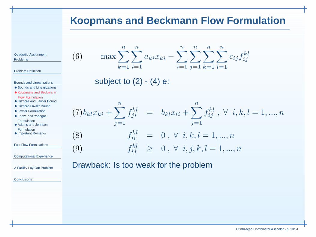
Koopmans and Beckmann Flow Formulation
maxn∑
k=1
n∑
i=1
akixki −n∑
i=1
n∑
j=1
n∑
k=1
n∑
l=1
cijfklij(6)
subject to (2) - (4) e:
bklxki +n∑
j=1
fklji = bklxli +
n∑
j=1
fklij , ∀ i, k, l = 1, ..., n(7)
fklii = 0 , ∀ i, k, l = 1, ..., n(8)
fklij ≥ 0 , ∀ i, j, k, l = 1, ..., n(9)
Drawback: Is too weak for the problem

Quadratic Assignment
Problems
Problem Definition
Bounds and Linearizations
•Bounds and Linearizations
•Koopmans and Beckmann
Flow Formulation•Gilmore and Lawler Bound
•Gilmore-Lawler Bound
•Lawler Formulation
•Frieze and Yadegar
Formulation•Adams and Johnson
Formulation• Important Remarks
Fast Flow Formulations
Computational Experience
A Facility Lay-Out Problem
Conclusions
Otimização Combinatória iacolor - p. 14/51
Gilmore and Lawler Bound
max p =n∑
k=1
n∑
i=1
(aki − λki)xki(10)
subject to:
n∑
k=1
xki = 1 , ∀ i = 1, ..., n(11)
n∑
i=1
xki = 1 , ∀ k = 1, ..., n(12)
xki ∈ {0, 1} , ∀ k, i = 1, ..., n.(13)

Quadratic Assignment
Problems
Problem Definition
Bounds and Linearizations
•Bounds and Linearizations
•Koopmans and Beckmann
Flow Formulation•Gilmore and Lawler Bound
•Gilmore-Lawler Bound
•Lawler Formulation
•Frieze and Yadegar
Formulation•Adams and Johnson
Formulation• Important Remarks
Fast Flow Formulations
Computational Experience
A Facility Lay-Out Problem
Conclusions
Otimização Combinatória iacolor - p. 15/51
Gilmore-Lawler Bound
λki = maxn∑
l=1
n∑
j=1
bklcijxlj(14)
subject to:
n∑
j=1
xlj = 1 , ∀l = 1, ..., n,(15)
n∑
l=1
xlj = 1 , ∀j = 1, ..., n,(16)
xki = 1 ,(17)
xlj ≥ 0 , ∀l, j = 1, ..., n.(18)
GLB takes n2 + 1 LAP solutions. It is tight for n ≤ 20.

Quadratic Assignment
Problems
Problem Definition
Bounds and Linearizations
•Bounds and Linearizations
•Koopmans and Beckmann
Flow Formulation•Gilmore and Lawler Bound
•Gilmore-Lawler Bound
•Lawler Formulation
•Frieze and Yadegar
Formulation•Adams and Johnson
Formulation• Important Remarks
Fast Flow Formulations
Computational Experience
A Facility Lay-Out Problem
Conclusions
Otimização Combinatória iacolor - p. 16/51
Lawler Formulation
maxn∑
k=1
n∑
i=1
akixki −n∑
k=1
n∑
l=1
n∑
i=1
n∑
j=1
dkiljykilj(19)
subject to (2) - (4) e:
n∑
k,l,i,j=1
ykilj = n2(20)
ykilj ≤ xki , ∀i, j, k, l = 1, ..., n, i 6= j, k 6= l(21)
ykilj ≤ xlj , ∀i, j, k, l = 1, ..., n, i 6= j, k 6= l(22)
ykilj ≥ 0 , ∀i, j, k, l = 1, ..., n, i 6= j, k 6= l(23)
The central idea: xkixlj = ykilj . Here dijkl = bklcij .Too large: n4 variables and n4 linking constraints.
Quadratic Assignment
Problems
Problem Definition
Bounds and Linearizations
•Bounds and Linearizations
•Koopmans and Beckmann
Flow Formulation•Gilmore and Lawler Bound
•Gilmore-Lawler Bound
•Lawler Formulation
•Frieze and Yadegar
Formulation•Adams and Johnson
Formulation• Important Remarks
Fast Flow Formulations
Computational Experience
A Facility Lay-Out Problem
Conclusions
Otimização Combinatória iacolor - p. 17/51
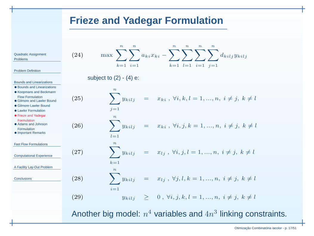
Frieze and Yadegar Formulation
max
n∑
k=1
n∑
i=1
akixki −
n∑
k=1
n∑
l=1
n∑
i=1
n∑
j=1
dkiljykilj(24)
subject to (2) - (4) e:
n∑
j=1
ykilj = xki , ∀i, k, l = 1, ..., n, i 6= j, k 6= l(25)
n∑
l=1
ykilj = xki , ∀i, j, k = 1, ..., n, i 6= j, k 6= l(26)
n∑
k=1
ykilj = xlj , ∀i, j, l = 1, ..., n, i 6= j, k 6= l(27)
n∑
i=1
ykilj = xlj , ∀j, l, k = 1, ..., n, i 6= j, k 6= l(28)
ykilj ≥ 0 , ∀i, j, k, l = 1, ..., n, i 6= j, k 6= l(29)
Another big model: n4 variables and 4n3 linking constraints.

Quadratic Assignment
Problems
Problem Definition
Bounds and Linearizations
•Bounds and Linearizations
•Koopmans and Beckmann
Flow Formulation•Gilmore and Lawler Bound
•Gilmore-Lawler Bound
•Lawler Formulation
•Frieze and Yadegar
Formulation•Adams and Johnson
Formulation• Important Remarks
Fast Flow Formulations
Computational Experience
A Facility Lay-Out Problem
Conclusions
Otimização Combinatória iacolor - p. 18/51
Adams and Johnson Formulation
maxn∑
k=1
n∑
i=1
akixki −n∑
k=1
n∑
l=1
n∑
i=1
n∑
j=1
dkiljykilj(30)
subject to (2) - (4) e:
n∑
j=1
ykilj = xki , ∀i, k, l = 1, ..., n, i 6= j, k 6= l(31)
n∑
l=1
ykilj = xki , ∀i, j, k = 1, ..., n, i 6= j, k 6= l(32)
ykilj = yljki , ∀i, j, k, l = 1, ..., n, i 6= j, k 6= l,(33)
ykilj ≥ 0 , ∀i, j, k, l = 1, ..., n, i 6= j, k 6= l(34)
Yet another large formulation: n4 variables and n4 + 2n3
linking constraints.As tight as Frieze and Yadegar formulation until we areaware.

Quadratic Assignment
Problems
Problem Definition
Bounds and Linearizations
•Bounds and Linearizations
•Koopmans and Beckmann
Flow Formulation•Gilmore and Lawler Bound
•Gilmore-Lawler Bound
•Lawler Formulation
•Frieze and Yadegar
Formulation•Adams and Johnson
Formulation• Important Remarks
Fast Flow Formulations
Computational Experience
A Facility Lay-Out Problem
Conclusions
Otimização Combinatória iacolor - p. 19/51
Important Remarks
• The main difficulty with QAP appears to be the excessivesymmetry.
• A good alternative to avoid this symmetry is to includelinear coefficients.
• It is necessary to find a formulation that balances boundquality and computational effort.
What if we could find a formulation that explores the non nulllinear term in the best way?What if this formulation combines a bound not so poor beingalso easy to solve?

Otimização Combinatória iacolor - p. 20/51
Fast Flow Formulations

Quadratic Assignment
Problems
Problem Definition
Bounds and Linearizations
Fast Flow Formulations
•Fast Flow Formulations
•Miranda and Luna:
Enhanced Flow
Formulation•Preprocessing for CPLEX
• Improving Bounds
•Re-interpreting Adams and
Johnson
Computational Experience
A Facility Lay-Out Problem
Conclusions
Otimização Combinatória iacolor - p. 21/51
Fast Flow Formulations
• Miranda and Luna Enhanced Flow Formulation.• Preprocessing for CPLEX.• Improving Bounds.• Re-interpreting Adams and Johnson.

Quadratic Assignment
Problems
Problem Definition
Bounds and Linearizations
Fast Flow Formulations
•Fast Flow Formulations
•Miranda and Luna:
Enhanced Flow
Formulation•Preprocessing for CPLEX
• Improving Bounds
•Re-interpreting Adams and
Johnson
Computational Experience
A Facility Lay-Out Problem
Conclusions
Otimização Combinatória iacolor - p. 22/51
Miranda and Luna:Enhanced Flow Formulation
maxn∑
k=1
n∑
i=1
akixki −∑
(i,j),i 6=j
∑
(k,l),k 6=l
cijfklij(35)
subject to (2) - (4) and:
−n∑
j=1
fklij = −bklxki , ∀ i, k, l = 1, ..., n, i 6= j , k 6= l(36)
n∑
i=1
fklij = bklxlj , ∀ j, k, l = 1, ..., n, i 6= j , k 6= l(37)
blk fklij = bklf
lkji , ∀ i, j, k, l = 1, ..., n, i 6= j , k 6= l(38)
fklij ≥ 0 , ∀ i, j, k, l = 1, ..., n, i 6= j , k 6= l(39)

Quadratic Assignment
Problems
Problem Definition
Bounds and Linearizations
Fast Flow Formulations
•Fast Flow Formulations
•Miranda and Luna:
Enhanced Flow
Formulation•Preprocessing for CPLEX
• Improving Bounds
•Re-interpreting Adams and
Johnson
Computational Experience
A Facility Lay-Out Problem
Conclusions
Otimização Combinatória iacolor - p. 23/51
Preprocessing for CPLEX
maxn∑
k=1
n∑
i=1
akixki −∑
i 6=j
∑
(k,l)∈φ
[cijbkl + cjiblk]fklij(40)
subject to (2) - (4) and:∑
j 6=i
fklij = xki , ∀ i = 1, ..., n, ∀(k, l) ∈ φ(41)
∑
i 6=j
fklij = xlj , ∀ j = 1, ..., n, ∀(k, l) ∈ φ(42)
fklij ≥ 0 , ∀ i, j = 1, ..., n, i 6= j , ∀(k, l) ∈ φ(43)
where:
φ = {(k, l)|k < l ∧ (bkl 6= 0 ∨ blk 6= 0)}(44)

Quadratic Assignment
Problems
Problem Definition
Bounds and Linearizations
Fast Flow Formulations
•Fast Flow Formulations
•Miranda and Luna:
Enhanced Flow
Formulation•Preprocessing for CPLEX
• Improving Bounds
•Re-interpreting Adams and
Johnson
Computational Experience
A Facility Lay-Out Problem
Conclusions
Otimização Combinatória iacolor - p. 24/51
Improving Bounds
If the bound is too poor in a given instance, we can add twofamilies of valid inequalities. These inequalities aretransliterations of Frieze and Yadegar work.
∑
k, (k,l)∈φ
fklij ≤ xlj , ∀ i, j = 1, ..., n, i 6= j , ∀l, (k, l) ∈ φ(45)
∑
l, (k,l)∈φ
fklij ≤ xki , ∀ i, j = 1, ..., n, i 6= j , ∀k, (k, l) ∈ φ

Quadratic Assignment
Problems
Problem Definition
Bounds and Linearizations
Fast Flow Formulations
•Fast Flow Formulations
•Miranda and Luna:
Enhanced Flow
Formulation•Preprocessing for CPLEX
• Improving Bounds
•Re-interpreting Adams and
Johnson
Computational Experience
A Facility Lay-Out Problem
Conclusions
Otimização Combinatória iacolor - p. 25/51
Re-interpreting Adams and Johnson
It is possible to re-interpret Adams and Johnson formulation as a
flow formulation. The idea is to take advantage of sparsity withoutcompromising LP bounds.
max
n∑
k=1
n∑
i=1
akixki −∑
i6=j
∑
(k,l)∈φ
[cijbkl + cjiblk]fklij(46)
subject to (2) - (4) and:∑
j 6=i
fklij = xki , ∀ i = 1, ..., n, ∀(k, l) ∈ φ(47)
∑
i6=j
fklij = xlj , ∀ j = 1, ..., n, ∀(k, l) ∈ φ(48)
∑
l∈φ|k<l
fklij +
∑
l∈φ|k>l
flkji ≤ xki , ∀ k ∈ K, ∀i 6= j(49)
fklij ≥ 0 , ∀ i, j = 1, ..., n, i 6= j , ∀(k, l) ∈ φ(50)

Otimização Combinatória iacolor - p. 26/51
Computational Experience

Quadratic Assignment
Problems
Problem Definition
Bounds and Linearizations
Fast Flow Formulations
Computational Experience
•Comparisons
•LP Bounds: AJ94 x ML04
•Computing Times (LP):
AJ94 x ML04.•Computing Times (MIP):
AJ94 x ML04.•LP Bounds: GLB x ML04
•LP Bounds: GLB x ML04
•Computing Times (MIP):
GLB x ML04.•After Preprocessing
•Tempos de Computação
(MIP): GLB x CML04•After Improving Bounds
•Limites de PL: GLB x
SCML04•Preprocessing Adams and
Johnson•Limites de PL: [AJ94]
Versus [CRLT-level1]
A Facility Lay-Out Problem
Conclusions
Otimização Combinatória iacolor - p. 27/51
Comparisons
• LP Bounds: AJ94 x ML04.• Computing Times: AJ94 x ML04.• LP Bounds: GLB x ML04.• Computing times: GLB x ML04.

Quadratic Assignment
Problems
Problem Definition
Bounds and Linearizations
Fast Flow Formulations
Computational Experience
•Comparisons
•LP Bounds: AJ94 x ML04
•Computing Times (LP):
AJ94 x ML04.•Computing Times (MIP):
AJ94 x ML04.•LP Bounds: GLB x ML04
•LP Bounds: GLB x ML04
•Computing Times (MIP):
GLB x ML04.•After Preprocessing
•Tempos de Computação
(MIP): GLB x CML04•After Improving Bounds
•Limites de PL: GLB x
SCML04•Preprocessing Adams and
Johnson•Limites de PL: [AJ94]
Versus [CRLT-level1]
A Facility Lay-Out Problem
Conclusions
Otimização Combinatória iacolor - p. 28/51
LP Bounds: AJ94 x ML04
Comparison of LP bounds.
0
0,1
0,2
0,3
0,4
0,5
0,6
0,7
0,8
0,9
1
chr12a
chr12b
chr12c
chr15a
chr15c
had12
had14
lipa10a
nug12
nug15
nug5
nug6
nug7
nug8
scr10
scr12
tai10a
tai10b
tai5a
tai6a
tai7a
tai8a
tai9a
Bound Quality
Flow form.
Adams & Johnson 94

Quadratic Assignment
Problems
Problem Definition
Bounds and Linearizations
Fast Flow Formulations
Computational Experience
•Comparisons
•LP Bounds: AJ94 x ML04
•Computing Times (LP):
AJ94 x ML04.•Computing Times (MIP):
AJ94 x ML04.•LP Bounds: GLB x ML04
•LP Bounds: GLB x ML04
•Computing Times (MIP):
GLB x ML04.•After Preprocessing
•Tempos de Computação
(MIP): GLB x CML04•After Improving Bounds
•Limites de PL: GLB x
SCML04•Preprocessing Adams and
Johnson•Limites de PL: [AJ94]
Versus [CRLT-level1]
A Facility Lay-Out Problem
Conclusions
Otimização Combinatória iacolor - p. 29/51
Computing Times (LP): AJ94 x ML04.
Comparison of LP computing times
1
10
100
1000
10000
100000
chr12a
chr12b
chr12c
chr15a
chr15c
had12
had14
lipa10a
nug12
nug15
nug5
nug6
nug7
nug8
scr10
scr12
tai10a
tai10b
tai5a
tai6a
tai7a
tai8a
tai9a
Time[s]
Flow form.
Adams & Johnson 94

Quadratic Assignment
Problems
Problem Definition
Bounds and Linearizations
Fast Flow Formulations
Computational Experience
•Comparisons
•LP Bounds: AJ94 x ML04
•Computing Times (LP):
AJ94 x ML04.•Computing Times (MIP):
AJ94 x ML04.•LP Bounds: GLB x ML04
•LP Bounds: GLB x ML04
•Computing Times (MIP):
GLB x ML04.•After Preprocessing
•Tempos de Computação
(MIP): GLB x CML04•After Improving Bounds
•Limites de PL: GLB x
SCML04•Preprocessing Adams and
Johnson•Limites de PL: [AJ94]
Versus [CRLT-level1]
A Facility Lay-Out Problem
Conclusions
Otimização Combinatória iacolor - p. 30/51
Computing Times (MIP): AJ94 x ML04.
Original Problem Variables p/q Flow form. Adams and Johnson
instance size Integer Continuous ratio time[s] time[s]
mchr12a 0.426 4 584
mchr12b 12 144 17424 0.383 5 516
mchr12c 0.314 3 803
mchr15a 0.631 16 14209
mchr15a 15 225 44100 0.856 6 10125
mchr15c 0.807 9 3058
mchr18a 0.564 116 *
mchr18b 18 324 93636 1.864 7 *
mchr20a 1.047 76 *
mchr20b 20 400 144400 0.824 47 *
mchr20c 1.056 108 *
mchr22a 22 484 213444 0.304 138 *
mchr22b 0.293 96 *

Quadratic Assignment
Problems
Problem Definition
Bounds and Linearizations
Fast Flow Formulations
Computational Experience
•Comparisons
•LP Bounds: AJ94 x ML04
•Computing Times (LP):
AJ94 x ML04.•Computing Times (MIP):
AJ94 x ML04.•LP Bounds: GLB x ML04
•LP Bounds: GLB x ML04
•Computing Times (MIP):
GLB x ML04.•After Preprocessing
•Tempos de Computação
(MIP): GLB x CML04•After Improving Bounds
•Limites de PL: GLB x
SCML04•Preprocessing Adams and
Johnson•Limites de PL: [AJ94]
Versus [CRLT-level1]
A Facility Lay-Out Problem
Conclusions
Otimização Combinatória iacolor - p. 31/51
LP Bounds: GLB x ML04
Flow Formulation Improvement from GLB X CV (%)
R2 = 0.8595
-30
-20
-10
0
10
20
30
1.5 2 2.5 3 3.5 4
CV (Flow Dominance)

Quadratic Assignment
Problems
Problem Definition
Bounds and Linearizations
Fast Flow Formulations
Computational Experience
•Comparisons
•LP Bounds: AJ94 x ML04
•Computing Times (LP):
AJ94 x ML04.•Computing Times (MIP):
AJ94 x ML04.•LP Bounds: GLB x ML04
•LP Bounds: GLB x ML04
•Computing Times (MIP):
GLB x ML04.•After Preprocessing
•Tempos de Computação
(MIP): GLB x CML04•After Improving Bounds
•Limites de PL: GLB x
SCML04•Preprocessing Adams and
Johnson•Limites de PL: [AJ94]
Versus [CRLT-level1]
A Facility Lay-Out Problem
Conclusions
Otimização Combinatória iacolor - p. 32/51
LP Bounds: GLB x ML04
Lower Bounds for p/q > 0
0.000
0.100
0.200
0.300
0.400
0.500
0.600
0.700
0.800
0.900
1.000
chr15a(0.72)
chr15b(1.76)
chr15c(1.56)
chr18a(1.57)
chr20b(1.72)
chr20c(0.91)
chr22a(1.7)
chr22b(1.32)
nug20(3.65)
nug30(1.91)
rqap32(0.7)
ste36a(0.99)
GLBFlow Form.

Quadratic Assignment
Problems
Problem Definition
Bounds and Linearizations
Fast Flow Formulations
Computational Experience
•Comparisons
•LP Bounds: AJ94 x ML04
•Computing Times (LP):
AJ94 x ML04.•Computing Times (MIP):
AJ94 x ML04.•LP Bounds: GLB x ML04
•LP Bounds: GLB x ML04
•Computing Times (MIP):
GLB x ML04.•After Preprocessing
•Tempos de Computação
(MIP): GLB x CML04•After Improving Bounds
•Limites de PL: GLB x
SCML04•Preprocessing Adams and
Johnson•Limites de PL: [AJ94]
Versus [CRLT-level1]
A Facility Lay-Out Problem
Conclusions
Otimização Combinatória iacolor - p. 33/51
Computing Times (MIP): GLB x ML04.
Original Instance Variables p/q Flow form. Branch-and-Bound
Instance size Integer Continuous ratio time[s] (GLB) time[s]
mchr15b 15 225 44100 0.726 36 0
mchr18a 18 324 93636 1.304 41 26
mchr20c 20 400 144400 0.707 54 75
mchr22a 22 484 213444 0.744 19 11
mnug20 20 400 144400 3.268 42 0
mnug30 30 900 756900 1.358 1779 23
rqap32 32 1024 984064 0.701 1964 2503
rqap33 33 1089 1115136 0.97 3236 3060
rqap34 34 1156 1258884 0.74 7207 7198
rqap35 35 1225 1416100 0.87 2610 16154
mste36a 0.687 2457 27974
mste36a 36 1296 1587600 1.199 2801 2925
mtho40 0.741 10532 *
mtho40 40 1600 2433600 1.040 7689 1984

Quadratic Assignment
Problems
Problem Definition
Bounds and Linearizations
Fast Flow Formulations
Computational Experience
•Comparisons
•LP Bounds: AJ94 x ML04
•Computing Times (LP):
AJ94 x ML04.•Computing Times (MIP):
AJ94 x ML04.•LP Bounds: GLB x ML04
•LP Bounds: GLB x ML04
•Computing Times (MIP):
GLB x ML04.•After Preprocessing
•Tempos de Computação
(MIP): GLB x CML04•After Improving Bounds
•Limites de PL: GLB x
SCML04•Preprocessing Adams and
Johnson•Limites de PL: [AJ94]
Versus [CRLT-level1]
A Facility Lay-Out Problem
Conclusions
Otimização Combinatória iacolor - p. 34/51
After Preprocessing
After Preprocessing:

Quadratic Assignment
Problems
Problem Definition
Bounds and Linearizations
Fast Flow Formulations
Computational Experience
•Comparisons
•LP Bounds: AJ94 x ML04
•Computing Times (LP):
AJ94 x ML04.•Computing Times (MIP):
AJ94 x ML04.•LP Bounds: GLB x ML04
•LP Bounds: GLB x ML04
•Computing Times (MIP):
GLB x ML04.•After Preprocessing
•Tempos de Computação
(MIP): GLB x CML04•After Improving Bounds
•Limites de PL: GLB x
SCML04•Preprocessing Adams and
Johnson•Limites de PL: [AJ94]
Versus [CRLT-level1]
A Facility Lay-Out Problem
Conclusions
Otimização Combinatória iacolor - p. 35/51
Tempos de Computação (MIP): GLB x CML04
Original Instance p/q Flow Form. Branch-And-Bound Compact Flow
Instance size ratio Time [s] (GLB) Time [s] Form. Time [s]
mchr15a 0.631 16 0 14
mchr15b 15 0.726 36 0 9
mchr15c 0.807 9 0 8
mchr18a 0.564 116 83 74
mchr18a 18 1.304 41 26 22
mchr20b 1.702 10 15 13
mchr20c 20 0.707 54 75 36
mchr22a 0.744 19 11 2
mchr22b 22 1.341 18 4 6
mnug20 20 3.268 42 0 4
mnug20 4.477 80 0 4
mnug30 30 1.358 1779 23 200
rqap32 32 0.701 1964 2503 1306
rqap33 33 0.97 3236 3060 1735
rqap34 34 0.74 7207 7198 3417
rqap35 35 0.87 2610 16154 1956
mste36a 36 1.199 2801 2925 325
mtho40 0.741 10532 * 5362
mtho40 40 1.040 7689 1984 1551
msko42 0.854 * * 16676
msko42 42 1.280 * * 3724

Quadratic Assignment
Problems
Problem Definition
Bounds and Linearizations
Fast Flow Formulations
Computational Experience
•Comparisons
•LP Bounds: AJ94 x ML04
•Computing Times (LP):
AJ94 x ML04.•Computing Times (MIP):
AJ94 x ML04.•LP Bounds: GLB x ML04
•LP Bounds: GLB x ML04
•Computing Times (MIP):
GLB x ML04.•After Preprocessing
•Tempos de Computação
(MIP): GLB x CML04•After Improving Bounds
•Limites de PL: GLB x
SCML04•Preprocessing Adams and
Johnson•Limites de PL: [AJ94]
Versus [CRLT-level1]
A Facility Lay-Out Problem
Conclusions
Otimização Combinatória iacolor - p. 36/51
After Improving Bounds
After Improving Bounds:

Quadratic Assignment
Problems
Problem Definition
Bounds and Linearizations
Fast Flow Formulations
Computational Experience
•Comparisons
•LP Bounds: AJ94 x ML04
•Computing Times (LP):
AJ94 x ML04.•Computing Times (MIP):
AJ94 x ML04.•LP Bounds: GLB x ML04
•LP Bounds: GLB x ML04
•Computing Times (MIP):
GLB x ML04.•After Preprocessing
•Tempos de Computação
(MIP): GLB x CML04•After Improving Bounds
•Limites de PL: GLB x
SCML04•Preprocessing Adams and
Johnson•Limites de PL: [AJ94]
Versus [CRLT-level1]
A Facility Lay-Out Problem
Conclusions
Otimização Combinatória iacolor - p. 37/51
Limites de PL: GLB x SCML04
ML04 Bound SCML04 Bound AJ94 Bound
instance lp bound time[s] Quality lp bound time[s] Quality lp bound time[s] Quality
chr12a.dat 8593.12 1 0.900 9246.67 1 0.968 9552 725 1.000
chr12b.dat 7184 1 0.737 9742 1 1.000 9742 508 1.000
chr12c.dat 10042.7 1 0.900 10121.1 1 0.907 11156 1068 1.000
chr15a.dat 8621.94 4 0.871 9295.33 4 0.939 9513 30146 0.961
chr15c.dat 9504 4 1.000 9504 4 1.000 9504 3622 1.000
had12.dat 894 17 0.541 1543.78 1414 0.934 1621.54 2533 0.982
had14.dat 1300.5 62 0.477 2583.07 9269 0.948 2666.12 14778 0.979
lipa10a.dat 318.8 4 0.674 448.123 161 0.947 473 50 1.000
nug12.dat 348 10 0.602 471.821 371 0.816 522.89 6597 0.905
nug15.dat 621 86 0.540 912.063 8790 0.793 1041 131923 0.905
nug5.dat 49 1 0.980 50 1 1.000 50 1 1.000
nug6.dat 72 1 0.837 80 1 0.930 86 1 1.000
nug7.dat 118 1 0.797 134.438 1 0.908 148 3 1.000
nug8.dat 154 1 0.720 191 3 0.893 203.5 17 0.951
scr10.dat 21958 2 0.816 24245.8 9 0.901 26873.1 269 0.998
scr12.dat 25474 5 0.811 27368.7 42 0.871 29827.3 4555 0.950
tai10a.dat 47953.3 3 0.355 112221 70 0.831 131098 160 0.971
tai10b.dat 855788 1 0.723 1139856.99 30 0.963 1176140 248 0.994
tai5a.dat 10747 1 0.833 12902 1 1.000 12902 1 1.000
tai6a.dat 21427.8 1 0.728 28013.4 1 0.952 29432 1 1.000
tai7a.dat 31730.1 1 0.588 47948 1 0.888 53976 1 1.000
tai8a.dat 41952.2 1 0.541 69705.1 1 0.899 77502 7 1.000
tai9a.dat 41816 2 0.442 83180.9 24 0.879 93501 37 0.988

Quadratic Assignment
Problems
Problem Definition
Bounds and Linearizations
Fast Flow Formulations
Computational Experience
•Comparisons
•LP Bounds: AJ94 x ML04
•Computing Times (LP):
AJ94 x ML04.•Computing Times (MIP):
AJ94 x ML04.•LP Bounds: GLB x ML04
•LP Bounds: GLB x ML04
•Computing Times (MIP):
GLB x ML04.•After Preprocessing
•Tempos de Computação
(MIP): GLB x CML04•After Improving Bounds
•Limites de PL: GLB x
SCML04•Preprocessing Adams and
Johnson•Limites de PL: [AJ94]
Versus [CRLT-level1]
A Facility Lay-Out Problem
Conclusions
Otimização Combinatória iacolor - p. 38/51
Preprocessing Adams and Johnson
Preprocessing AJ94:

Quadratic Assignment
Problems
Problem Definition
Bounds and Linearizations
Fast Flow Formulations
Computational Experience
•Comparisons
•LP Bounds: AJ94 x ML04
•Computing Times (LP):
AJ94 x ML04.•Computing Times (MIP):
AJ94 x ML04.•LP Bounds: GLB x ML04
•LP Bounds: GLB x ML04
•Computing Times (MIP):
GLB x ML04.•After Preprocessing
•Tempos de Computação
(MIP): GLB x CML04•After Improving Bounds
•Limites de PL: GLB x
SCML04•Preprocessing Adams and
Johnson•Limites de PL: [AJ94]
Versus [CRLT-level1]
A Facility Lay-Out Problem
Conclusions
Otimização Combinatória iacolor - p. 39/51
Limites de PL: [AJ94] Versus [CRLT-level1]
Instance Compact RLT level1 RLT level 1 [AJ94]
name size lp bound time [s] bound quality lp bound time [s] bound quality
nug5 5 50.0 0 1.0000 50.0 1 1.0000
tai5a 5 12,902.0 0 1.0000 12,902.0 1 1.0000
nug6 6 86.0 0 1.0000 86.0 1 1.0000
tai6a 6 29,432.0 1 1.0000 29,432.0 1 1.0000
nug7 7 148.0 1 1.0000 148.0 3 1.0000
tai7a 7 53,976.0 1 1.0000 53,976.0 1 1.0000
nug8 8 202.6 6 0.9469 203.5 17 0.9509
tai8a 8 77,502.0 5 1.0000 77,502.0 7 1.0000
tai9a 9 93,501.0 26 0.9882 93,501.0 37 0.9882
lipa10a 10 473.0 50 1.0000 47 3.0 50 1.0000
scr10 10 26,659.0 12 0.9902 26,873.1 269 0.9982
tai10a 10 131,053.0 86 0.9706 131,098.0 160 0.9709
tai10b 10 1,172,043.4 47 0.9901 1,176,140.0 248 0.9936
chr12a 12 9,552.0 2 1.0000 9,552.0 725 1.0000
chr12b 12 9,742.0 1 1.0000 9,742.0 508 1.0000
chr12c 12 10,927.3 1 0.9795 11,156.0 1,068 1.0000
had12 12 1,621.5 1,633 0.9816 1,621.5 2,533 0.9816
nug12 12 522.7 308 0.9043 522.9 6,597 0.9047
scr12 12 29,766.5 59 0.9477 29,827.3 4,555 0.9496
had14 14 2,666.1 12,044 0.9788 2,666.1 14,778 0.9788
chr15a 15 9,456.5 3 0.9556 9,513.0 30,146 0.9613
chr15c 15 9,504.0 2 1.0000 9,504.0 3,622 1.0000
nug15 15 1,040.3 7,895 0.9046 1,041.0 131,923 0.9052
nug20 20 2,180.4 157,424 0.8484 2,181.6 2,310,985 0.8489

Otimização Combinatória iacolor - p. 40/51
A Facility Lay-Out Problem

Quadratic Assignment
Problems
Problem Definition
Bounds and Linearizations
Fast Flow Formulations
Computational Experience
A Facility Lay-Out Problem
•Problem Description
•Problem Description
•Problem Description
•The Original Lay-out and
Production Flows•Assignment Costs
•The Mass Flow Matrix
•The grid on the Shop Floor
•The Final Lay-out and
Production Flows•Achieved Improvements
Conclusions
Otimização Combinatória iacolor - p. 41/51
Problem Description
• SILA BRASIL is an automotive components manufacturerin Belo Horizonte, Minas Gerais, Brasil.
• SILA is a part of FIAT S.A. supply chain.
• Its expertise is the manufacturing of precision componentsfor 16-valve engines and other machine elements.

Quadratic Assignment
Problems
Problem Definition
Bounds and Linearizations
Fast Flow Formulations
Computational Experience
A Facility Lay-Out Problem
•Problem Description
•Problem Description
•Problem Description
•The Original Lay-out and
Production Flows•Assignment Costs
•The Mass Flow Matrix
•The grid on the Shop Floor
•The Final Lay-out and
Production Flows•Achieved Improvements
Conclusions
Otimização Combinatória iacolor - p. 42/51
Problem Description
• The main problem in its former lay-out was the excessivetraffic of vehicles inside his plant to transport raw materials.
• His lay-out was organized in two major areas: docking areaand cellular manufacturing area

Quadratic Assignment
Problems
Problem Definition
Bounds and Linearizations
Fast Flow Formulations
Computational Experience
A Facility Lay-Out Problem
•Problem Description
•Problem Description
•Problem Description
•The Original Lay-out and
Production Flows•Assignment Costs
•The Mass Flow Matrix
•The grid on the Shop Floor
•The Final Lay-out and
Production Flows•Achieved Improvements
Conclusions
Otimização Combinatória iacolor - p. 43/51
Problem Description
SILA has 13 manufacturing cells:
• 1. Cutting• 2. Push-Pull setup• 3. Push-Pull shifts• 4. Pull shifts• 5. Shift Gears PALIO• 6. Shift Gears UNO• 7. Shift Gears STILO/IDEA• 8. Shift Gears DOBLO• 9. Shift Gears DUCATO• 10. Shift Gears MAREA• 11. Inflow area (docking)• 12. Finished product area (docking)• 13. Tubular elements area (docking)

Quadratic Assignment
Problems
Problem Definition
Bounds and Linearizations
Fast Flow Formulations
Computational Experience
A Facility Lay-Out Problem
•Problem Description
•Problem Description
•Problem Description
•The Original Lay-out and
Production Flows•Assignment Costs
•The Mass Flow Matrix
•The grid on the Shop Floor
•The Final Lay-out and
Production Flows•Achieved Improvements
Conclusions
Otimização Combinatória iacolor - p. 44/51
The Original Lay-out and Production Flows
Fluxo ComponentesFluxo PI�s �Área de CorteFluxo PI�s �Push-PullFluxo PI�s �PreparaçãoFluxo Produto Acabado
Fluxo ComponentesFluxo PI�s �Área de CorteFluxo PI�s �Push-PullFluxo PI�s �PreparaçãoFluxo Produto Acabado

Quadratic Assignment
Problems
Problem Definition
Bounds and Linearizations
Fast Flow Formulations
Computational Experience
A Facility Lay-Out Problem
•Problem Description
•Problem Description
•Problem Description
•The Original Lay-out and
Production Flows•Assignment Costs
•The Mass Flow Matrix
•The grid on the Shop Floor
•The Final Lay-out and
Production Flows•Achieved Improvements
Conclusions
Otimização Combinatória iacolor - p. 45/51
Assignment Costs

Quadratic Assignment
Problems
Problem Definition
Bounds and Linearizations
Fast Flow Formulations
Computational Experience
A Facility Lay-Out Problem
•Problem Description
•Problem Description
•Problem Description
•The Original Lay-out and
Production Flows•Assignment Costs
•The Mass Flow Matrix
•The grid on the Shop Floor
•The Final Lay-out and
Production Flows•Achieved Improvements
Conclusions
Otimização Combinatória iacolor - p. 46/51
The Mass Flow Matrix

Quadratic Assignment
Problems
Problem Definition
Bounds and Linearizations
Fast Flow Formulations
Computational Experience
A Facility Lay-Out Problem
•Problem Description
•Problem Description
•Problem Description
•The Original Lay-out and
Production Flows•Assignment Costs
•The Mass Flow Matrix
•The grid on the Shop Floor
•The Final Lay-out and
Production Flows•Achieved Improvements
Conclusions
Otimização Combinatória iacolor - p. 47/51
The grid on the Shop Floor
D

Quadratic Assignment
Problems
Problem Definition
Bounds and Linearizations
Fast Flow Formulations
Computational Experience
A Facility Lay-Out Problem
•Problem Description
•Problem Description
•Problem Description
•The Original Lay-out and
Production Flows•Assignment Costs
•The Mass Flow Matrix
•The grid on the Shop Floor
•The Final Lay-out and
Production Flows•Achieved Improvements
Conclusions
Otimização Combinatória iacolor - p. 48/51
The Final Lay-out and Production Flows
Fluxo ComponentesFluxo PI�s �Área de Corte
Fluxo PI�s �Push-PullFluxo PI�s �Preparação
Fluxo Produto Acabado
Fluxo ComponentesFluxo PI�s �Área de Corte
Fluxo PI�s �Push-PullFluxo PI�s �Preparação
Fluxo Produto Acabado

Quadratic Assignment
Problems
Problem Definition
Bounds and Linearizations
Fast Flow Formulations
Computational Experience
A Facility Lay-Out Problem
•Problem Description
•Problem Description
•Problem Description
•The Original Lay-out and
Production Flows•Assignment Costs
•The Mass Flow Matrix
•The grid on the Shop Floor
•The Final Lay-out and
Production Flows•Achieved Improvements
Conclusions
Otimização Combinatória iacolor - p. 49/51
Achieved Improvements
• 12% of effective improvement of productivity.
• 15% of effective reduction of shop floor area.

Otimização Combinatória iacolor - p. 50/51
Conclusions

Quadratic Assignment
Problems
Problem Definition
Bounds and Linearizations
Fast Flow Formulations
Computational Experience
A Facility Lay-Out Problem
Conclusions
•Conclusions
Otimização Combinatória iacolor - p. 51/51
Conclusions
• Miranda and Luna Fast Flow Formulation is more sensitiveto the presence of linear terms.
• The impact of preprocessing is huge for Adams andJohnson Formulation.
• The use of a linear term appears to be a clue to breakdown the excessive symmetry of QAP.
• Interpreting the QAP as a network flow problem enablesthe solution of practical engineering problems.
Recommended


![QAP Summary [R]](https://img.dokumen.tips/doc/110x75/577cc1221a28aba7119253d1/qap-summary-r.jpg)