Factor Models for Asset Returns
Eric Zivot
University of Washington
BlackRock Alternative Advisors
March 14, 2011
Outline
1. Introduction
2. Factor Model Specification
3. Macroeconomic factor models
4. Fundamental factor models
5. Statistical factor models
Introduction
Factor models for asset returns are used to
• Decompose risk and return into explanable and unexplainable components
• Generate estimates of abnormal return
• Describe the covariance structure of returns
• Predict returns in specified stress scenarios
• Provide a framework for portfolio risk analysis
Three Types of Factor Models
1. Macroeconomic factor model
(a) Factors are observable economic and financial time series
2. Fundamental factor model
(a) Factors are created from observerable asset characteristics
3. Statistical factor model
(a) Factors are unobservable and extracted from asset returns
Factor Model Specification
The three types of multifactor models for asset returns have the general form
Rit = αi + β1if1t + β2if2t + · · ·+ βKifKt + εit (1)
= αi + β0ift + εit
• Rit is the simple return (real or in excess of the risk-free rate) on asset i
(i = 1, . . . , N) in time period t (t = 1, . . . , T ),
• fkt is the kth common factor (k = 1, . . . ,K),
• βki is the factor loading or factor beta for asset i on the kth factor,
• εit is the asset specific factor.
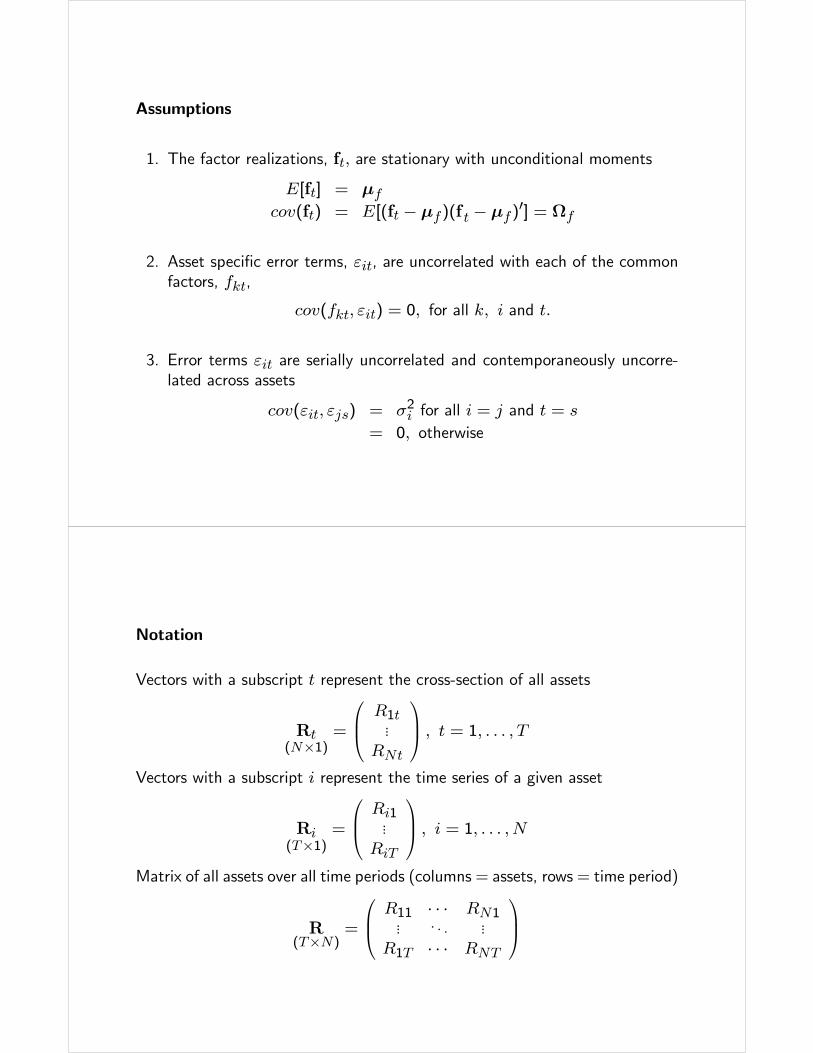
Assumptions
1. The factor realizations, ft, are stationary with unconditional moments
E[ft] = μfcov(ft) = E[(ft − μf)(f t − μf)
0] = Ωf
2. Asset specific error terms, εit, are uncorrelated with each of the common
factors, fkt,
cov(fkt, εit) = 0, for all k, i and t.
3. Error terms εit are serially uncorrelated and contemporaneously uncorre-
lated across assets
cov(εit, εjs) = σ2i for all i = j and t = s
= 0, otherwise
Notation
Vectors with a subscript t represent the cross-section of all assets
Rt(N×1)
=
⎛⎜⎝ R1t...
RNt
⎞⎟⎠ , t = 1, . . . , T
Vectors with a subscript i represent the time series of a given asset
Ri(T×1)
=
⎛⎜⎝ Ri1...
RiT
⎞⎟⎠ , i = 1, . . . , N
Matrix of all assets over all time periods (columns = assets, rows = time period)
R(T×N)
=
⎛⎜⎝ R11 · · · RN1... . . . ...
R1T · · · RNT
⎞⎟⎠
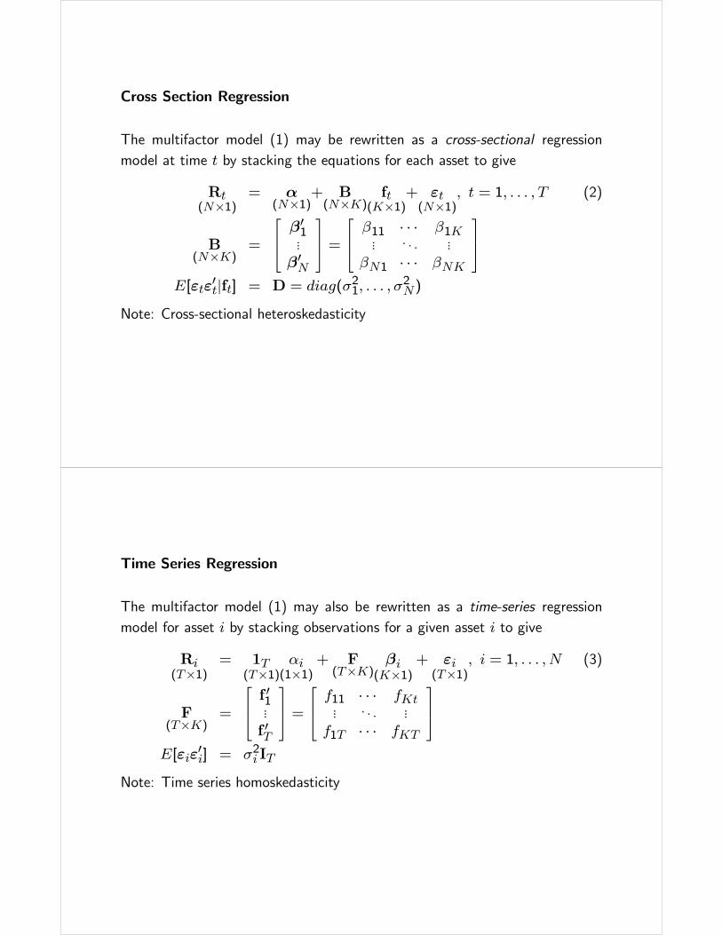
Cross Section Regression
The multifactor model (1) may be rewritten as a cross-sectional regression
model at time t by stacking the equations for each asset to give
Rt(N×1)
= α(N×1)
+ B(N×K)
ft(K×1)
+ εt(N×1)
, t = 1, . . . , T (2)
B(N×K)
=
⎡⎢⎣ β01...
β0N
⎤⎥⎦ =⎡⎢⎣ β11 · · · β1K
... . . . ...
βN1 · · · βNK
⎤⎥⎦E[εtε
0t|ft] = D = diag(σ21, . . . , σ
2N)
Note: Cross-sectional heteroskedasticity
Time Series Regression
The multifactor model (1) may also be rewritten as a time-series regression
model for asset i by stacking observations for a given asset i to give
Ri(T×1)
= 1T(T×1)
αi(1×1)
+ F(T×K)
βi(K×1)
+ εi(T×1)
, i = 1, . . . , N (3)
F(T×K)
=
⎡⎢⎣ f 01...f 0T
⎤⎥⎦ =⎡⎢⎣ f11 · · · fKt
... . . . ...
f1T · · · fKT
⎤⎥⎦E[εiε
0i] = σ2i IT
Note: Time series homoskedasticity
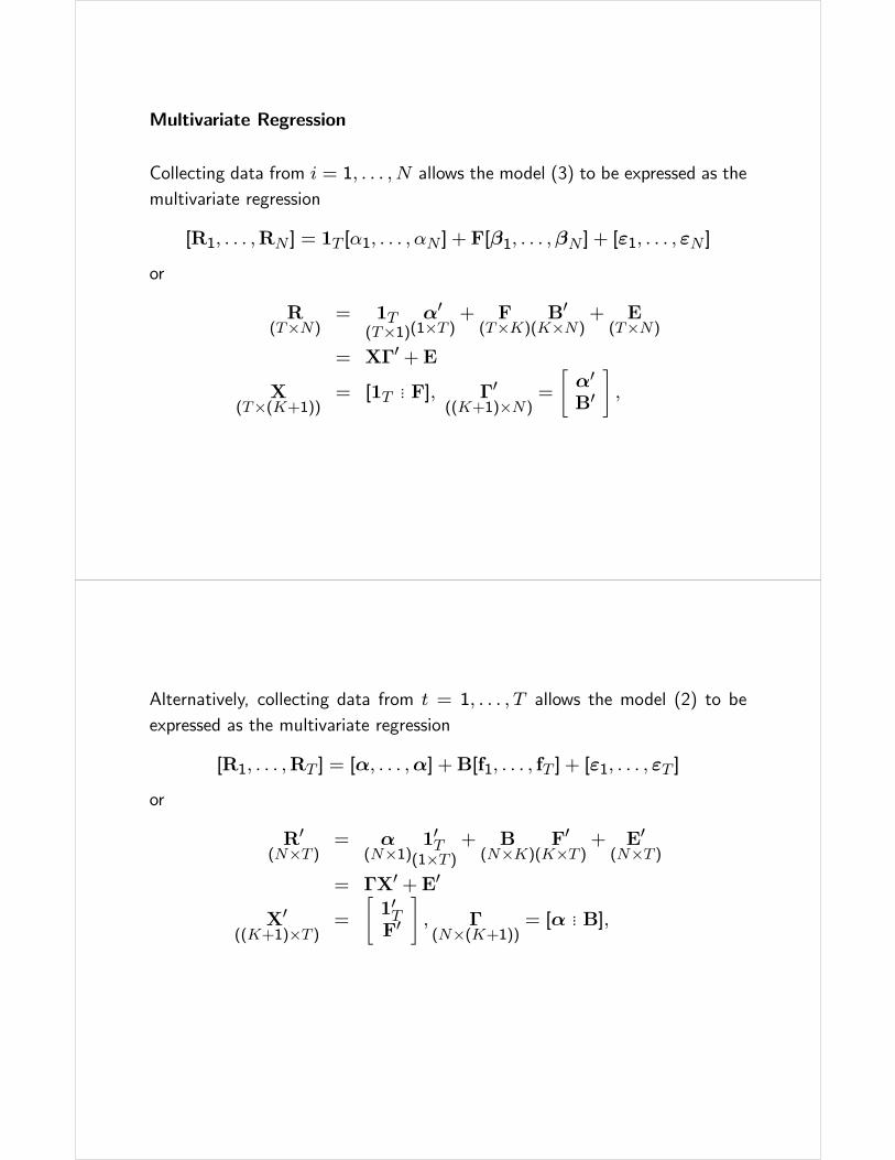
Multivariate Regression
Collecting data from i = 1, . . . , N allows the model (3) to be expressed as the
multivariate regression
[R1, . . . ,RN ] = 1T [α1, . . . , αN ] + F[β1, . . . ,βN ] + [ε1, . . . , εN ]
or
R(T×N)
= 1T(T×1)
α0(1×T )
+ F(T×K)
B0(K×N)
+ E(T×N)
= XΓ0 +E
X(T×(K+1))
= [1T... F], Γ0
((K+1)×N)=
"α0B0
#,
Alternatively, collecting data from t = 1, . . . , T allows the model (2) to be
expressed as the multivariate regression
[R1, . . . ,RT ] = [α, . . . ,α] +B[f1, . . . , fT ] + [ε1, . . . , εT ]
or
R0(N×T )
= α(N×1)
10T(1×T )
+ B(N×K)
F0(K×T )
+ E0(N×T )
= ΓX0 + E0
X0((K+1)×T )
=
"10TF0
#, Γ(N×(K+1))
= [α ... B],
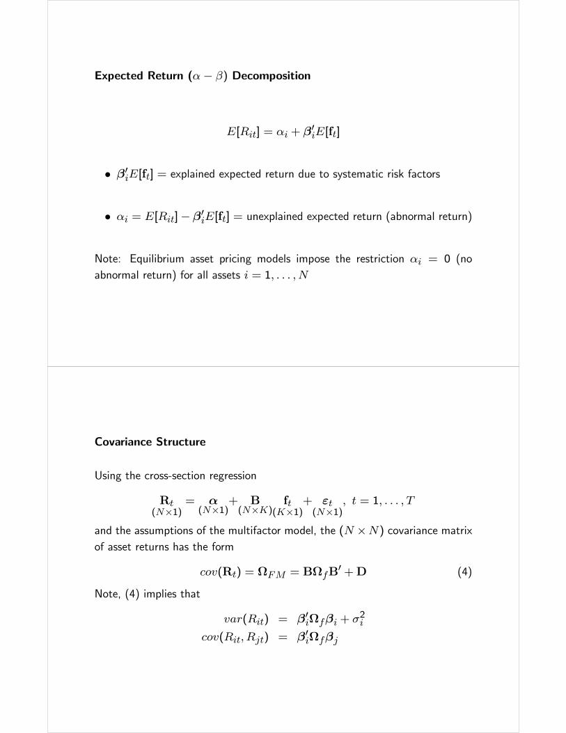
Expected Return (α− β) Decomposition
E[Rit] = αi + β0iE[ft]
• β0iE[ft] = explained expected return due to systematic risk factors
• αi = E[Rit]− β0iE[ft] = unexplained expected return (abnormal return)
Note: Equilibrium asset pricing models impose the restriction αi = 0 (no
abnormal return) for all assets i = 1, . . . , N
Covariance Structure
Using the cross-section regression
Rt(N×1)
= α(N×1)
+ B(N×K)
ft(K×1)
+ εt(N×1)
, t = 1, . . . , T
and the assumptions of the multifactor model, the (N ×N) covariance matrix
of asset returns has the form
cov(Rt) = ΩFM = BΩfB0 +D (4)
Note, (4) implies that
var(Rit) = β0iΩfβi + σ2i
cov(Rit,Rjt) = β0iΩfβj

Portfolio Analysis
Let w = (w1, . . . , wn) be a vector of portfolio weights (wi = fraction of
wealth in asset i). If Rt is the (N × 1) vector of simple returns then
Rp,t = w0Rt =
NXi=1
wiRit
Portfolio Factor Model
Rt = α+Bf t + εt⇒Rp,t = w0α+w0Bf t +w0εt = αp + β0pft + εp,t
αp = w0α, β0p = w0B, εp,t = w0εtvar(Rp,t) = β0pΩfβp + var(εp,t) = w
0BΩfB0w+w0Dw
Active and Static Portfolios
• Active portfolios have weights that change over time due to active assetallocation decisions
• Static portfolios have weights that are fixed over time (e.g. equally weightedportfolio)
• Factor models can be used to analyze the risk of both active and staticportfolios
Macroeconomic Factor Models
Rit = αi + β0ift + εit
ft = observed economic/financial time series
Econometric problems:
• Choice of factors
• Estimate factor betas, βi, and residual variances, σ2i , using time seriesregression techniques.
• Estimate factor covariance matrix, Ωf , from observed history of factors
Shape’s Single Factor Model
Sharpe’s single factor model is a macroeconomic factor model with a single
market factor:
Rit = αi + βiRMt + εit, i = 1, . . . , N ; t = 1, . . . , T (5)
where RMt denotes the return or excess return (relative to the risk-free rate)
on a market index (typically a value weighted index like the S&P 500 index) in
time period t.
Risk-adusted expected return and abnormal return
E[Rit] = βiE[RMt]
αi = E[Rit]− βiE[RMt]
Covariance matrix of assets
ΩFM = σ2Mββ0 +D (6)
where
σ2M = var(RMt)
β = (β1, . . . , βN)0
D = diag(σ21, . . . , σ2N),
σ2i = var(εit)
Estimation
Because RMt is observable, the parameters βi and σ2i of the single factor
model (5) for each asset can be estimated using time series regression (i.e.,
ordinary least squares) giving
Ri = bαi1T +RMbβi + bεi, i = 1, . . . , Nbβi = dcov(Rit,RMt)/dvar(RMt) = σiM/σ2Mbαi = Ri − βiRMbσ2i =
1
T − 2bε0ibεiThe estimated single factor model covariance matrix is
bΩFM = bσ2M bβ bβ0 +cD

Remarks
1. Computational efficiency may be obtained by using multivariate regression.
The coefficients αi and βi and the residual variances σ2i may be computed
in one step in the multivariate regression model
R = XΓ0 +E
The multivariate OLS estimator of Γ0 isbΓ0 = (X0X)−1X0R0.
The estimate of the residual covariance matrix is
bΣ =1
T − 2bE0 bE
where E = R−XΓ0 is the multivariate least squares residual matrix. Thediagonal elements of bΣ are the diagonal elements of cD.
2. The R2 from the time series regression is a measure of the proportion of
“market” risk, and 1−R2 is a measure of asset specific risk. Additionally,bσi is a measure of the typical size of asset specific risk. Given the variancedecomposition
var(Rit) = β2i var(RMt) + var(εit) = β2i σ2M + σ2i
R2 can be estimated using
R2 =β2i σ2Mdvar(Rit)
3. Robust regression techniques can be used to estimate βi and σ2i . Also, a
robust estimate of σ2M could be computed.
4. The single factor covariance matrix (6) is constant over time. This may
not be a good assumption. There are several ways to allow (6) to vary
over time. In general, βi, σ2i and σ
2M can be time varying. That is,
βi = βit, σ2i = σ2it, σ
2M = σ2Mt.
To capture time varying betas, rolling regression or Kalman filter techniques
could be used. To capture conditional heteroskedasticity, GARCH models
may be used for σ2it and σ2Mt. One may also use exponential weights in
computing estimates of βit, σ2it and σ2Mt. A time varying factor model
covariance matrix is
bΩFM,t = bσ2Mtbβtbβ0t +cDt,
General Multi-factor Model
Model specifies K observable macro-variables
Rit = αi + β0ift + εit
• Chen, Roll and Ross (1986) provides a description of commonly usedmacroeconomic factors for equity. Lo (2008) discusses hedge funds.
• Sometimes the macroeconomic factors are standardized to have mean zeroand a common scale.
• The factors must be stationary (not trending).
• Sometimes the factors are made orthogonal.
Estimation
Because the factor realizations are observable, the parameter matrices B and
D of the model may be estimated using time series regression:
Ri = bαi1T + Fbβi + bεi = Xγ + bεi, i = 1, . . . , NX = [1T
... F], γ = (αi, β0i)0 = (X0X)−1X0Ribσ2i =
1
T −K − 1bε0ibεiThe covariance matrix of the factor realizations may be estimated using the
time series sample covariance matrix
bΩf =1
T − 1TXt=1
(ft − f)(ft − f)0, f =1
T
TXt=1
ft
The estimated multifactor model covariance matrix is thenbΩFM = bB bΩfbB0 +cD (7)
Remarks
1. As with the single factor model, robust regression may be used to compute
βi and σ2i . A robust covariance matrix estimator may also be used to
compute and estimate of Ωf .
2. ΩFM can be made time varying by allowing βi,Ωf and σ2i (i = 1, . . . , N)
to be time varying
Example: Estimation of Single Index Model in R using investment data from
Berndt (1991).
Fundamental Factor Models
Fundamental factor models use observable asset specific characteristics (fun-
damentals) like industry classification, market capitalization, style classification
(value, growth) etc. to determine the common risk factors.
• Factor betas are constructed from observable asset characteristics (i.e., Bis known)
• Factor realizations, ft, are estimated/constructed for each t given B
• In practice, fundamental factor models are estimated in two ways.

BARRA Approach
• This approach was pioneered by Bar Rosenberg, founder of BARRA Inc.,and is discussed at length in Grinold and Kahn (2000), Conner et al (2010),
and Cariño et al (2010).
• In this approach, the observable asset specific fundamentals (or some trans-formation of them) are treated as the factor betas, βi, which are time
invariant.
• The factor realizations at time t, ft, are unobservable. The econometricproblem is then to estimate the factor realizations at time t given the factor
betas. This is done by running T cross-section regressions.
Fama-French Approach
• This approach was introduced by Eugene Fama and Kenneth French (1992).
• For a given observed asset specific characteristic, e.g. size, they determinedfactor realizations using a two step process. First they sorted the cross-
section of assets based on the values of the asset specific characteristic.
Then they formed a hedge portfolio which is long in the top quintile of the
sorted assets and short in the bottom quintile of the sorted assets. The
observed return on this hedge portfolio at time t is the observed factor
realization for the asset specific characteristic. This process is repeated for
each asset specific characteristic.
• Given the observed factor realizations for t = 1, . . . , T, the factor betas
for each asset are estimated using N time series regressions.
BARRA-type Single Factor Model
Consider a single factor model in the form of a cross-sectional regression at
time t
Rt(N×1)
= β(N×1)
ft(1×1)
+ εt(N×1)
, t = 1, . . . , T
• β is an N×1 vector of observed values of an asset specific attribute (e.g.,market capitalization, industry classification, style classification)
• ft is an unobserved factor realization.
• var(ft) = σ2f ; cov(ft, εit) = 0, for all i, t; var(εit) = σ2i , i = 1, . . . , N.
Estimation
For each time period t = 1, . . . T, the vector of factor betas, β, is treated as
data and the factor realization ft, is the parameter to be estimated. Since the
error term εt is heteroskedastic, efficient estimation of ft is done by weighted
least squares (WLS) (assuming the asset specific variances σ2i are known)
ft,wls = (β0D−1β)−1β0D−1Rt, t = 1, . . . , T (8)
D = diag(σ21, . . . , σ2N)
Note 1: σ2i can be consistently estimated and a feasible WLS estimate can be
computed
ft,fwls = (β0D−1β)−1β0D−1Rt, t = 1, . . . , T
D = diag(σ21, . . . , σ2N)
Note 2: Other weights besides σ2i could be used
Factor Mimicking Portfolio
The WLS estimate of ft in (8) has an interesting interpretation as the return
on a portfolio h = (h1, . . . , hN)0 that solves
minh
1
2h0Dh subject to h0β = 1
The portfolio h minimizes asset return residual variance subject to having unit
exposure to the attribute β and is given by
h0 = (β0D−1β)−1β0D−1
The estimated factor realization is then the portfolio return
ft,wls = h0Rt
When the portfolio h is normalized such thatPNi hi = 1, it is referred to as a
factor mimicking portfolio.
BARRA-type Industry Factor Model
Consider a stylized BARRA-type industry factor model with K mutually ex-
clusive industries. The factor sensitivities βik in (1) for each asset are time
invariant and of the form
βik = 1 if asset i is in industry k
= 0, otherwise
and fkt represents the factor realization for the kth industry in time period t.
• The factor betas are dummy variables indicating whether a given asset isin a particular industry.
• The estimated value of fkt will be equal to the weighted average excessreturn in time period t of the firms operating in industry k.

Industry Factor Model Regression
The industry factor model with K industries is summarized as
Rit = βi1f1t + · · ·+ βiKfKt + εit, i = 1, . . . , N ; t = 1, . . . , T
var(εit) = σ2i , i = 1, . . . , N
cov(εit, fjt) = 0, j = 1, . . . ,K; i = 1, . . . , N
cov(fit, fjt) = σfij, i, j = 1, . . . ,K
where
βik = 1 if asset i is in industry k (k = 1, . . . ,K)
= 0, otherwise
It is assumed that there are Nk firms in the kth industry suchPKk=1Nk = N .
Estimation of Industry Factor Model Factors
Consider the cross-section regression at time t
Rt = β1f1t + · · ·+ βKfKt + εt,
= Bf t + εt
E[εtε0t] = D, cov(ft) = Ωf
Since the industries are mutually exclusive it follows that
β0jβk = Nk for j = k, 0 otherwise
An unbiased but inefficient estimate of the factor realizations ft can be obtained
by OLS:
bft,OLS = (B0B)−1B0Rt =
⎛⎜⎝ bf1t,OLS...bfKt,OLS
⎞⎟⎠ =⎛⎜⎜⎜⎝
1N1
PN1i=1R
1it
...1NK
PNKi=1R
Kit
⎞⎟⎟⎟⎠
Estimation of Factor Realization Covariance Matrix
Given (bf1,OLS, . . . , bfT,OLS), the covariance matrix of the industry factors maybe computed as the time series sample covariance
bΩFOLS =
1
T − 1TXt=1
(bft,OLS − fOLS)(bft,OLS − fOLS)0,fOLS =
1
T
TXt=1
bft,OLS
Estimation of Residual Variances
The residual variances, var(εit) = σ2i , can be estimated from the time series
of residuals from the T cross-section regressions as follows. Let bεt,OLS, t =1, . . . , T , denote the (N × 1) vector of OLS residuals, and let bεit,OLS denotethe ith row of bεt,OLS. Then σ2i may be estimated using
bσ2i,OLS =1
T − 1TXt=1
(bεit,OLS − εi,OLS)2, i = 1, . . . , N
εi,OLS =1
T
TXt=1
bεit,OLS
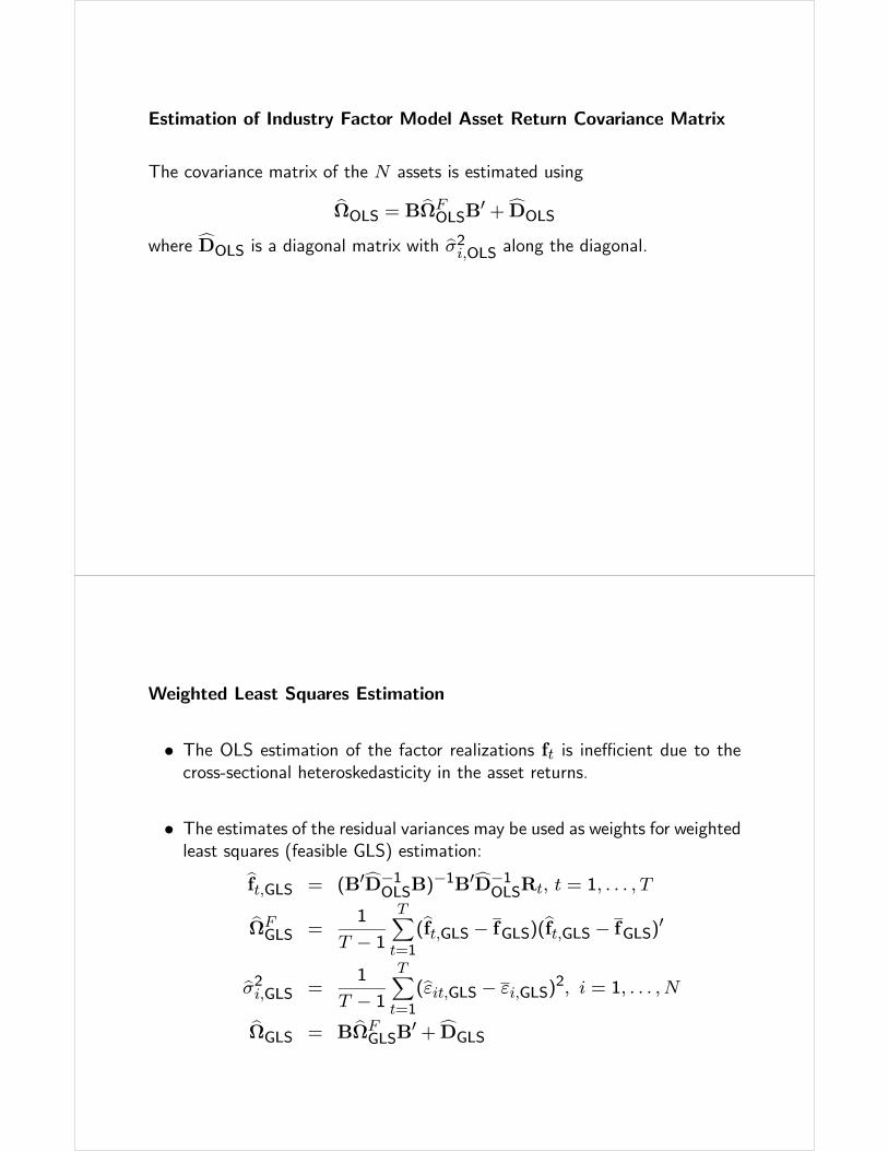
Estimation of Industry Factor Model Asset Return Covariance Matrix
The covariance matrix of the N assets is estimated using
bΩOLS = B bΩFOLSB
0 +cDOLSwhere cDOLS is a diagonal matrix with bσ2i,OLS along the diagonal.
Weighted Least Squares Estimation
• The OLS estimation of the factor realizations ft is inefficient due to thecross-sectional heteroskedasticity in the asset returns.
• The estimates of the residual variances may be used as weights for weightedleast squares (feasible GLS) estimation:bft,GLS = (B0cD−1OLSB)−1B0cD−1OLSRt, t = 1, . . . , T
bΩFGLS =
1
T − 1TXt=1
(bft,GLS − fGLS)(bft,GLS − fGLS)0bσ2i,GLS =
1
T − 1TXt=1
(bεit,GLS − εi,GLS)2, i = 1, . . . , N
bΩGLS = B bΩFGLSB
0 +cDGLS

Statistical Factor Models for Returns
• In statistical factor models, the factor realizations ft in (1) are not directlyobservable and must be extracted from the observable returns Rt using
statistical methods. The primary methods are factor analysis and principal
components analysis.
• Traditional factor analysis and principal component analysis are usuallyapplied to extract the factor realizations if the number of time series ob-
servations, T , is greater than the number of assets, N .
• If N > T , then the sample covariance matrix of returns becomes singular
which complicates traditional factor and principal components analysis. In
this case, the method of asymptotic principal component analysis is more
appropriate.
Sample Covariance Matrices
Traditional factor and principal component analysis is based on the (N ×N)
sample covariance matrix
bΩN(N×N)
=1
TR0R
where R is the (N × T ) matrix of observed returns.
Asymptotic principal component analysis is based on the (T × T ) covariance
matrix bΩT(T×T )
=1
NRR0.

Factor Analysis
Traditional factor analysis assumes a time invariant orthogonal factor structure
Rt(N×1)
= μ(N×1)
+ B(N×K)
ft(K×1)
+ εt(N×1)
(9)
cov(ft, εs) = 0, for all t, s
E[ft] = E[εt] = 0
var(ft) = IK
var(εt) = D
where D is a diagonal matrix with σ2i along the diagonal. Then, the return
covariance matrix, Ω, may be decomposed as
Ω = BB0+D
Hence, the K common factors ft account for all of the cross covariances of
asset returns.
Variance Decomposition
For a given asset i, the return variance variance may be expressed as
var(Rit) =KXj=1
β2ij + σ2i
• variance portion due to common factors, PKj=1 β
2ij, is called the commu-
nality,
• variance portion due to specific factors, σ2i , is called the uniqueness.
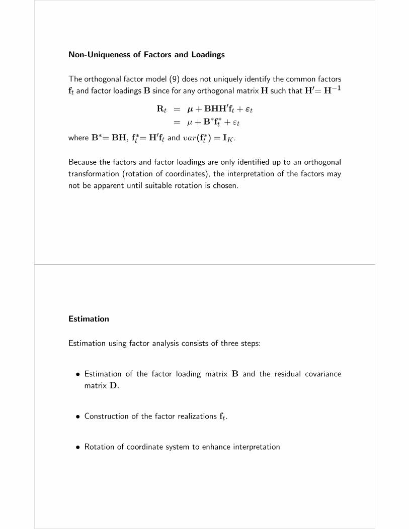
Non-Uniqueness of Factors and Loadings
The orthogonal factor model (9) does not uniquely identify the common factors
ft and factor loadingsB since for any orthogonal matrixH such thatH0= H−1
Rt = μ+BHH0ft + εt
= μ+B∗f∗t + εt
where B∗= BH, f∗t = H0ft and var(f∗t ) = IK.
Because the factors and factor loadings are only identified up to an orthogonal
transformation (rotation of coordinates), the interpretation of the factors may
not be apparent until suitable rotation is chosen.
Estimation
Estimation using factor analysis consists of three steps:
• Estimation of the factor loading matrix B and the residual covariance
matrix D.
• Construction of the factor realizations ft.
• Rotation of coordinate system to enhance interpretation

Maximum Likelihood Estimation of B and D
Maximum likelihood estimation of B andD is performed under the assumption
that returns are jointly normally distributed and temporally iid.
Given estimates bB and cD, an empirical version of the factor model (2) may beconstructed as
Rt − bμ = bBft + bεt (10)
where bμ is the sample mean vector of Rt. The error terms in (10) are het-
eroskedastic so that OLS estimation is inefficient.
Estimation of Factor Realizations ft
Using (10), the factor realizations in a given time period t, ft, can be estimated
using the cross-sectional feasible weighted least squares (FWLS) regression
bft,fwls = ( bB0cD−1 bB)−1 bB0cD−1(Rt − bμ) (11)
Performing this regression for t = 1, . . . , T times gives the time series of factor
realizations (bf1, . . . , bfT ).The factor model estimated covariance matrix is then given by
bΩF = bB bB0 +cD
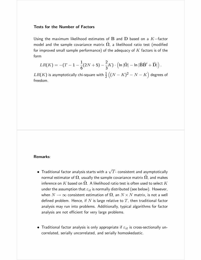
Tests for the Number of Factors
Using the maximum likelihood estimates of B and D based on a K−factormodel and the sample covariance matrix bΩ, a likelihood ratio test (modifiedfor improved small sample performance) of the adequacy of K factors is of the
form
LR(K) = −(T − 1− 16(2N + 5)− 2
3K) ·
³ln | bΩ|− ln | bB bB0 +cD|´ .
LR(K) is asymptotically chi-square with 12
³(N −K)2 −N −K
´degrees of
freedom.
Remarks:
• Traditional factor analysis starts with a√T - consistent and asymptotically
normal estimator of Ω, usually the sample covariance matrix bΩ, and makesinference onK based on bΩ. A likelihood ratio test is often used to selectKunder the assumption that εit is normally distributed (see below). However,
when N →∞ consistent estimation of Ω, an N×N matrix, is not a well
defined problem. Hence, if N is large relative to T , then traditional factor
analysis may run into problems. Additionally, typical algorithms for factor
analysis are not efficient for very large problems.
• Traditional factor analysis is only appropriate if εit is cross-sectionally un-correlated, serially uncorrelated, and serially homoskedastic.
Principal Components
• Principal component analysis (PCA) is a dimension reduction techniqueused to explain the majority of the information in the sample covariance
matrix of returns.
• With N assets there are N principal components, and these principal
components are just linear combinations of the returns.
• The principal components are constructed and ordered so that the firstprincipal component explains the largest portion of the sample covariance
matrix of returns, the second principal component explains the next largest
portion, and so on. The principal components are constructed to be or-
thogonal to each other and to be normalized to have unit length.
• In terms of a multifactor model, the K most important principal compo-
nents are the factor realizations. The factor loadings on these observed
factors can then be estimated using regression techniques.
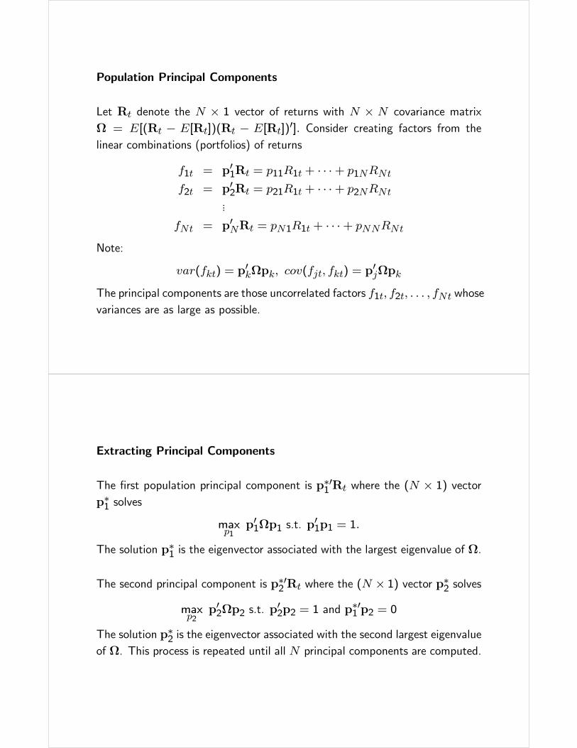
Population Principal Components
Let Rt denote the N × 1 vector of returns with N × N covariance matrix
Ω = E[(Rt − E[Rt])(Rt − E[Rt])0]. Consider creating factors from the
linear combinations (portfolios) of returns
f1t = p01Rt = p11R1t + · · ·+ p1NRNt
f2t = p02Rt = p21R1t + · · ·+ p2NRNt...
fNt = p0NRt = pN1R1t + · · ·+ pNNRNt
Note:
var(fkt) = p0kΩpk, cov(fjt, fkt) = p
0jΩpk
The principal components are those uncorrelated factors f1t, f2t, . . . , fNt whose
variances are as large as possible.
Extracting Principal Components
The first population principal component is p∗01Rt where the (N × 1) vectorp∗1 solves
maxp1
p01Ωp1 s.t. p01p1 = 1.
The solution p∗1 is the eigenvector associated with the largest eigenvalue of Ω.
The second principal component is p∗02Rt where the (N × 1) vector p∗2 solves
maxp2
p02Ωp2 s.t. p02p2 = 1 and p∗01 p2 = 0
The solution p∗2 is the eigenvector associated with the second largest eigenvalueof Ω. This process is repeated until all N principal components are computed.
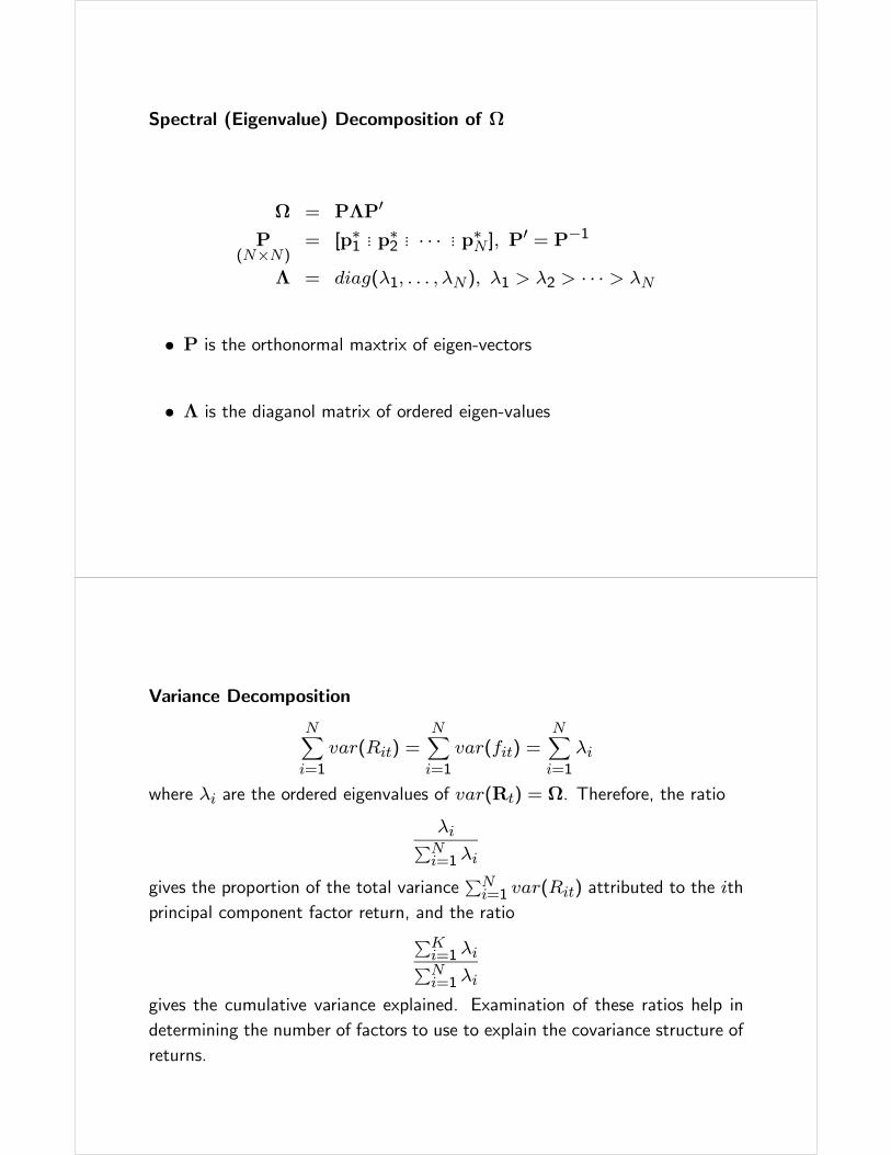
Spectral (Eigenvalue) Decomposition of Ω
Ω = PΛP0
P(N×N)
= [p∗1 ... p∗2 ... · · · ... p∗N ], P0 = P−1
Λ = diag(λ1, . . . , λN), λ1 > λ2 > · · · > λN
• P is the orthonormal maxtrix of eigen-vectors
• Λ is the diaganol matrix of ordered eigen-values
Variance Decomposition
NXi=1
var(Rit) =NXi=1
var(fit) =NXi=1
λi
where λi are the ordered eigenvalues of var(Rt) = Ω. Therefore, the ratio
λiPNi=1 λi
gives the proportion of the total variancePNi=1 var(Rit) attributed to the ith
principal component factor return, and the ratioPKi=1 λiPNi=1 λi
gives the cumulative variance explained. Examination of these ratios help in
determining the number of factors to use to explain the covariance structure of
returns.
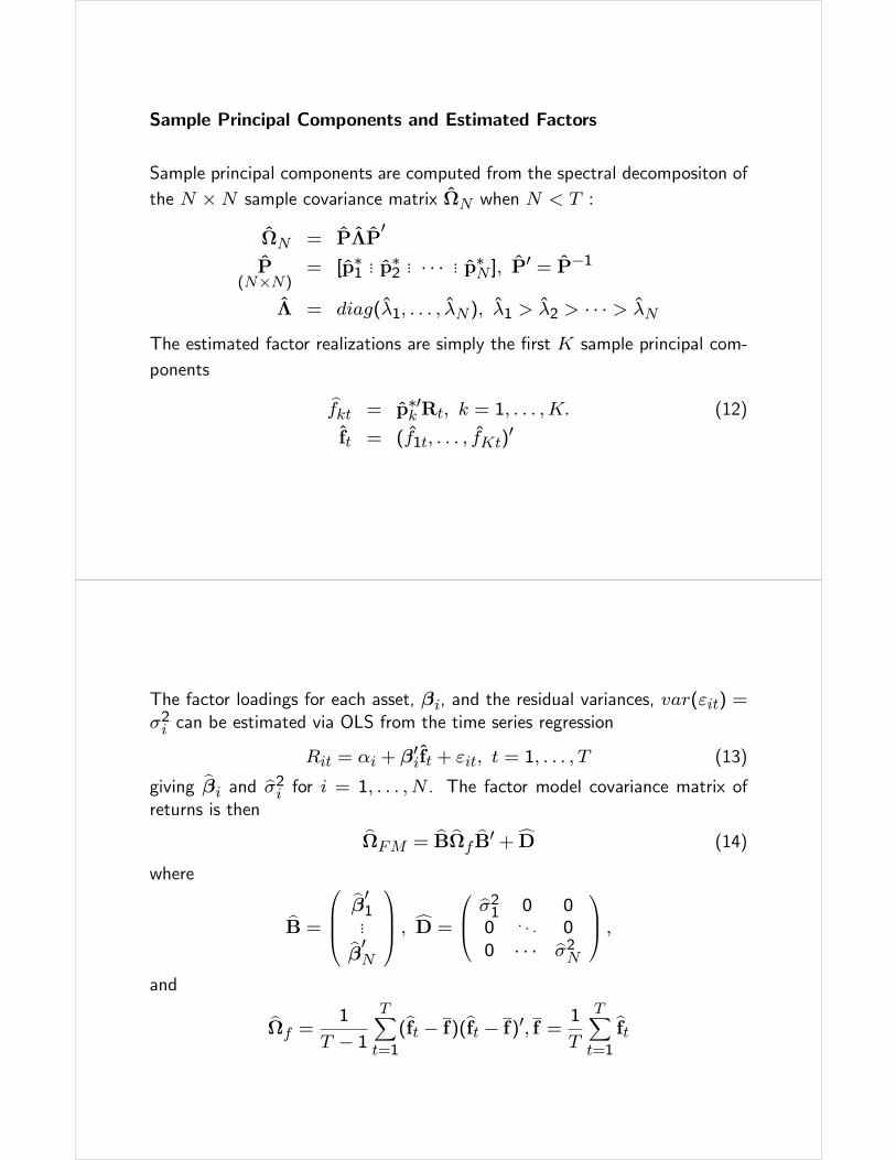
Sample Principal Components and Estimated Factors
Sample principal components are computed from the spectral decompositon of
the N ×N sample covariance matrix ΩN when N < T :
ΩN = PΛP0
P(N×N)
= [p∗1 ... p∗2 ... · · · ... p∗N ], P0 = P−1
Λ = diag(λ1, . . . , λN), λ1 > λ2 > · · · > λN
The estimated factor realizations are simply the first K sample principal com-
ponents
bfkt = p∗0kRt, k = 1, . . . ,K. (12)
ft = (f1t, . . . , fKt)0
The factor loadings for each asset, βi, and the residual variances, var(εit) =
σ2i can be estimated via OLS from the time series regression
Rit = αi + β0ift + εit, t = 1, . . . , T (13)
giving bβi and bσ2i for i = 1, . . . , N . The factor model covariance matrix of
returns is then bΩFM = bB bΩfbB0 +cD (14)
where
bB =⎛⎜⎜⎝
bβ01...bβ0N⎞⎟⎟⎠ , cD =
⎛⎜⎝ bσ21 0 0
0 . . . 0
0 · · · bσ2N⎞⎟⎠ ,
and
bΩf =1
T − 1TXt=1
(bft − f)(bft − f)0, f = 1
T
TXt=1
bft
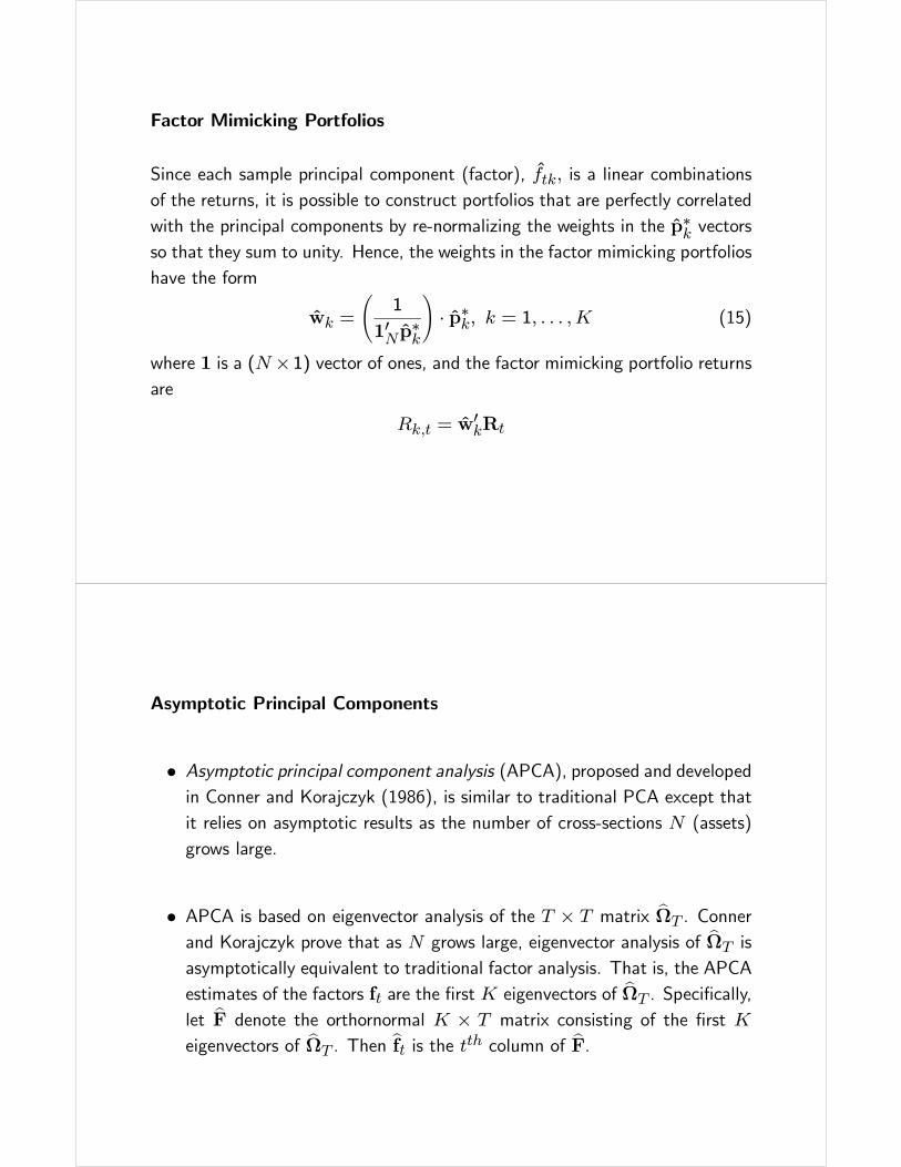
Factor Mimicking Portfolios
Since each sample principal component (factor), ftk, is a linear combinations
of the returns, it is possible to construct portfolios that are perfectly correlated
with the principal components by re-normalizing the weights in the p∗k vectorsso that they sum to unity. Hence, the weights in the factor mimicking portfolios
have the form
wk =
Ã1
10N p∗k
!· p∗k, k = 1, . . . ,K (15)
where 1 is a (N×1) vector of ones, and the factor mimicking portfolio returnsare
Rk,t = w0kRt
Asymptotic Principal Components
• Asymptotic principal component analysis (APCA), proposed and developedin Conner and Korajczyk (1986), is similar to traditional PCA except that
it relies on asymptotic results as the number of cross-sections N (assets)
grows large.
• APCA is based on eigenvector analysis of the T × T matrix bΩT . Conner
and Korajczyk prove that as N grows large, eigenvector analysis of bΩT is
asymptotically equivalent to traditional factor analysis. That is, the APCA
estimates of the factors ft are the first K eigenvectors of bΩT . Specifically,
let bF denote the orthornormal K × T matrix consisting of the first K
eigenvectors of bΩT . Thenbft is the tth column of bF.
The main advantages of the APCA approach are:
• It works in situations where the number of assets, N , is much greaterthan the number of time periods, T . Eigenvectors of the smaller T × T
matrix bΩT only need to be computed, whereas with traditional principal
component analysis eigenvalues of the larger N ×N matrix bΩN need to
be computed.
• The method allows for an approximate factor structure of returns. In anapproximate factor structure, the asset specific error terms εit are allowed
to be contemporaneously correlated, but this correlation is not allowed
to be too large across the cross section of returns. Allowing an approxi-
mate factor structure guards against picking up local factors, e.g. industry
factors, as global common factors.
Determining the Number of Factors
• In practice, the number of factors is unknown and must be determinedfrom the data.
• If traditional factor analysis is used, then there is a likelihood ratio test forthe number of factors. However, this test will not work if N > T .
• Connor and Korajczyk (1993) described a procedure for determining thenumber of factors in an approximate factor model that is valid for N > T .
Bai and Ng (2002) proposed an information criteria that is easier and more
reliable to use.

Bai and Ng Method
Bai and Ng (2002) propose some panel Cp (Mallows-type) information criteria
for choosing the number of factors. Their criteria are based on the observation
that eigenvector analysis on bΩT orbΩN solves the least squares problem
minβi,f t
(NT )−1NXi=1
TXt=1
(Rit − αi − β0ift)2
Bai and Ng’s model selection or information criteria are of the form
IC(K) = bσ2(K) +K · g(N,T )
bσ2(K) =1
N
NXi=1
bσ2iwhere bσ2(K) is the cross-sectional average of the estimated residual variancesfor each asset based on a model with K factors and g(N,T ) is a penalty
function depending only on N and T .
The preferred model is the one which minimizes the information criteria IC(K)
over all values of K < Kmax. Bai and Ng consider several penalty functions
and the preferred criteria are
PCp1(K) = bσ2(K) +K · bσ2(Kmax)µN + T
NT
¶· ln
µNT
N + T
¶,
PCp2(K) = bσ2(K) +K · bσ2(Kmax)µN + T
NT
¶· ln
³C2NT
´,
CNT = min(√N,√T )
Algorithm
First, select a number Kmax indicating the maximum number of factors to be
considered. Then for each value of K < Kmax, do the following:
1. Extract realized factors bft using the method of APCA.2. For each asset i, estimate the factor model
Rit = αi + β0ibfKt + εit,
where the superscript K indicates that the regression has K factors, using
time series regression and compute the residual variances
bσ2i (K) = 1
T −K − 1TXt=1
bε2it.
3. Compute the cross-sectional average of the estimated residual variances
for each asset based on a model with K factors
bσ2(K) = 1
N
NXi=1
bσ2i (K)4. Compute the cross-sectional average of the estimated residual variances
for each asset based on a model with Kmax factors, bσ2(Kmax).5. Compute the information criteria PCp1(K) and PCp2(K).
6. Select the value of K that minimized either PCp1(K) or PCp2(K).
Bai and Ng perform an extensive simulation study and find that the selection
criteria PCp1 and PCp2 yield high precision when min(N,T ) > 40.
Recommended