Factor Model Based Risk Measurement andMeasurement and
ManagementR/Finance 2011: Applied Finance with R
April 30 2011April 30, 2011
Eric ZivotRobert Richards Chaired Professor of EconomicsRobert Richards Chaired Professor of Economics
Adjunct Professor, Departments of Applied Mathematics, Finance and Statistics, University of Washington

Risk Measurement and ManagementRisk Measurement and Management• Quantify asset and portfolio exposures to risk
factorsfactors– Equity, rates, credit, volatility, currency
St l h i d t– Style, geography, industry, • Quantify asset and portfolio risk
– SD, VaR, ETL• Perform risk decomposition
– Contribution of risk factors, contribution of constituent assets to portfolio risk
• Stress testing and scenario analysis© Eric Zivot 2011

Asset Level Linear Factor ModelAsset Level Linear Factor Model1 1 , it i i t ik kt itR F Fα β β ε= + + + +
1i i t it
i t t Tα ε′= + +β F1, , ; , ,
~ ( , )i
t F F
i n t t T= =
F μ Σ… …
2,
( )
~ (0, )t F F
it iεε σ
μ
cov( , ) 0 for all , , and
cov( ) 0 for andjt isF j i s t
i j s t
ε
ε ε
=
= ≠© Eric Zivot 2011
cov( , ) 0 for , and it js i j s tε ε = ≠

Performance AttributionPerformance Attribution
][][][ FEFERE ββ +++ ][][][ 11 ktiktiiit FEFERE ββα +++=
E t d t d t t ti “b t ”
][][ 11 ktikti FEFE ββ ++
Expected return due to systematic “beta” exposure
11 ktikti ββ
Expected return due to firm specific “alpha”
])[][(][ 11 ktiktiiti FEFERE ββα ++−=
© Eric Zivot 2011

Factor Model CovarianceFactor Model Covariance
t t= + +R α B F εt
var( ) ′= = +R Σ BΣ B D
11 1 1t tn knn k n××× × ×
t
2 2,1 ,
var( )
( , , )t FM
ndiagε
ε ε εσ σ
= = +
=FR Σ BΣ B D
D …
cov( , ) var( )it jt i t j i jR R ′ ′= = Fβ F β β Σ βNote:2,var( )
it jt i t j i j
it i i iR εσ′= +F
Fβ Σ β
© Eric Zivot 2011

Portfolio Linear Factor ModelPortfolio Linear Factor Model1( , , ) portfolio weightsnw w ′= =w …
11, 0 for 1, ,
n
i ii
w w i n=
= ≥ =∑ …
,p t t t tR ′ ′ ′ ′= = + +w R w α w BF w ε
1i=
1 1 1 1
n n n n
i it i i i i t i iti i i i
w R w w wα ε= = = =
′= = + +∑ ∑ ∑ ∑β F1 1 1 1
,
i i i i
p p t p tα ε′= + +β F
© Eric Zivot 2011

Risk MeasuresRisk MeasuresReturn Standard Deviation (SD, aka active risk)
( )1/22( )t FSD R εσ σ′= = +βΣ β
1( ) 0 01 0 10VaR q F α α−= = ≤ ≤Value-at-Risk (VaR)
( ), 0.01 0.10 of return t
VaR q FF CDF R
α α α α= = ≤ ≤
=Expected Tail Loss (ETL)
[ | ]ETL E R R VaR= ≤
© Eric Zivot 2011
[ | ]t tETL E R R VaRα α= ≤

Risk MeasuresRisk Measures25 5% VaR5% ETL
520
Den
sity
1015
5 ± SD
0
© Eric Zivot 2011Returns
-0.15 -0.10 -0.05 0.00 0.05

Tail Risk Measures: Non-Normal Distributions
• Asset returns are typically non-normalAsset returns are typically non-normal• Many possible univariate non-normal
distributionsdistributions– Student’s-t, skewed-t, generalized hyperbolic,
Gram Charlier α stable generalized Pareto etcGram-Charlier, α-stable, generalized Pareto, etc.• Need multivariate non-normal distributions for
tf li l i d i k b d tiportfolio analysis and risk budgeting.• Large number of assets, small samples and
unequal histories make multivariate modeling difficult © Eric Zivot 2011

Factor Model Monte Carlo (FMMC)Factor Model Monte Carlo (FMMC)
• Use fitted factor model to simulate pseudoUse fitted factor model to simulate pseudo asset return data preserving empirical characteristics of risk factors and residualscharacteristics of risk factors and residuals– Use full data for factors and unequal history for
assets to deal with missing dataassets to deal with missing data• Estimate tail risk and related measures non-
parametrically from simulated return dataparametrically from simulated return data
© Eric Zivot 2011

Simulation Algorithmg• Simulate B values of the risk factors by re-sampling
from full sample empirical distribution:from full sample empirical distribution:
• Simulate B values of the factor model residuals from{ }1 , , B
* *F F…• Simulate B values of the factor model residuals from
fitted non-normal distribution:
{ }* *ˆ ˆ 1i nε ε• Create factor model returns from factor models fit over
truncated samples simulated factor variables drawn
{ }1 , , , 1, ,i iB i nε ε =… …
truncated samples, simulated factor variables drawn from full sample and simulated residuals:
* * *ˆˆ ˆ 1 ; 1R t B i nα ε′= + + = =β F
© Eric Zivot 2011
, 1, , ; 1, ,it i i t itR t B i nα ε= + + = =β F … …

What to do with ?{ } { } { }* *ˆ, , ,B B B
it it itR ε*FWhat to do with ?
• Backfill missing asset performance
{ } { } { }1 1 1, , ,it it itt t t
R ε= = =
F
Backfill missing asset performance• Compute asset and portfolio performance
measures (e g Sharpe ratios)measures (e.g., Sharpe ratios)• Compute non-parametric estimates of asset
d f li il i kand portfolio tail risk measures• Compute non-parametric estimates of asset
and factor contributions to portfolio tail risk measures
© Eric Zivot 2009
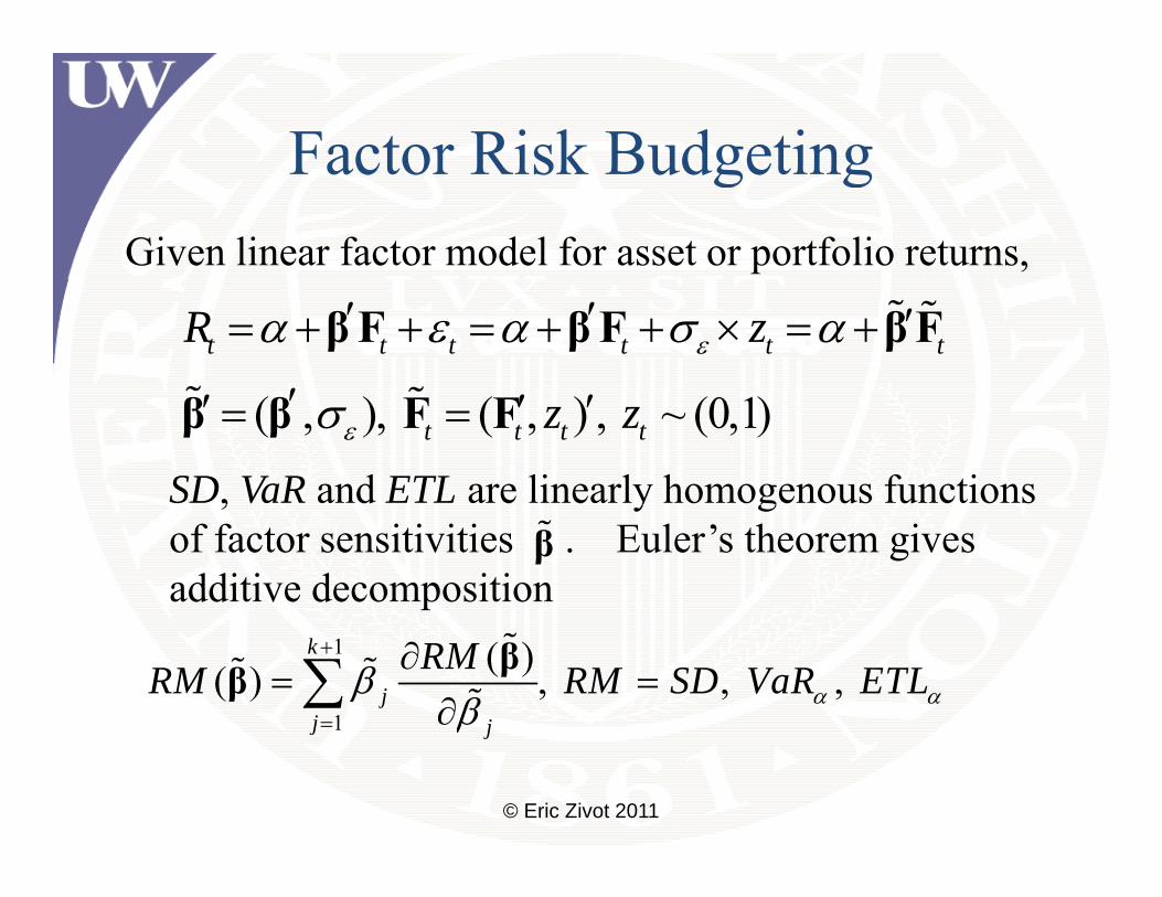
Factor Risk BudgetingFactor Risk BudgetingGiven linear factor model for asset or portfolio returns,
t t t t t tR zεα ε α σ α′ ′ ′= + + = + + × = +
′
βF βF βF
SD, VaR and ETL are linearly homogenous functions
( , ), ( , ) , ~ (0,1)t t t tz zεσ′′ ′ ′= =β β F F
, y gof factor sensitivities . Euler’s theorem gives additive decomposition
β
1
1
( )( ) , , , k
jj j
RMRM RM SD VaR ETLα αββ
+
=
∂= =
∂∑ ββ
© Eric Zivot 2011
j jβ

Factor Contributions to RiskFactor Contributions to Risk
Marginal Contribution to Risk of factor j:
( )
j
RMβ
∂∂
β
Contribution to Risk f f t j
( )j
RMββ
∂∂
β
of factor j:
Percent Contribution to Risk
jβ∂
( ) ( )RM RMβ ∂ β βof factor j:
( )jj
RMββ∂
β
© Eric Zivot 2011
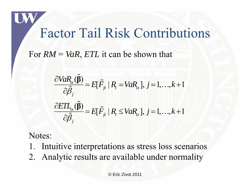
Factor Tail Risk ContributionsFactor Tail Risk ContributionsFor RM = VaR, ETL it can be shown that
( ) [ | ] 1 1VaR E F R VaR j kα∂= = = +
β [ | ], 1, , 1
( ) [ | ] 1 1
jt tj
E F R VaR j k
ETL E F R V R j k
α
α
β= = = +
∂
∂≤
β
…
( ) [ | ], 1, , 1jt tj
E F R VaR j kααβ
= ≤ = +∂
β …
NNotes: 1. Intuitive interpretations as stress loss scenarios2 Analytic results are available under normality
© Eric Zivot 2011
2. Analytic results are available under normality

Semi-Parametric EstimationSemi Parametric EstimationFactor Model Monte Carlo semi-parametric estimates
{ }* *1ˆ[ | ] 1B
E F R V R F V R R V R≤ ≤∑ { }
{ }1
* *
[ | ] 1
1ˆ
jt t jt tt
B
E F R VaR F VaR R VaRmα α αε ε
=
= = ⋅ − ≤ ≤ +∑
∑ { }* *
1
1ˆ[ | ] 1[ ]jt t jt t
tE F R VaR F R VaR
Bα αα =
≤ = ⋅ ≤∑
© Eric Zivot 2011

Hedge fund returns and 5% VaR Violations
0.00
Ret
urns
1998 2000 2002 2004 2006
-0.1
0
5% VaRIndex
Risk factor returns when fund return <= 5% VaR
5% VaR
000.
06
turn
s
-0.0
60.
0
Ret
© Eric Zivot 2011
1998 2000 2002 2004 2006
IndexFactor marginal contribution to 5% ETL

Portfolio Risk BudgetingPortfolio Risk BudgetingGiven portfolio returns,
,1
n
p t t i iti
R w R=
′= =∑w R
SD, VaR and ETL are linearly homogenous functions of portfolio weights w. Euler’s theorem gives p g gadditive decomposition
1
( )( ) , , , n
ii i
RMRM w RM SD VaR ETLw α α
=
∂= =
∂∑ ww
© Eric Zivot 2011

Fund Contributions to Portfolio RiskFund Contributions to Portfolio Risk
Marginal Contribution to Risk of asset i:
( )
i
RMw
∂∂
w
Contribution to Risk f t i
( )i
i
RMww
∂∂
w
of asset i:
Percent Contribution to Risk ( ) ( )RMw RM∂ w wof asset i: ( )ii
w RMw∂
w
© Eric Zivot 2011

Portfolio Tail Risk ContributionsPortfolio Tail Risk ContributionsFor RM = VaR, ETL it can be shown that
( ) [ | ( )] 1VaR E R R VaR i nα∂= = =
w w,[ | ( )], 1, ,
( ) [ | ( )] 1
it p ti
E R R VaR i nw
ETL E R R VaR i n
α
α
= = =∂
∂= ≤ =
w
w w
…
,[ | ( )], 1, ,it p ti
E R R VaR i nw α= ≤ =∂
w …
N A l i l il bl d liNote: Analytic results are available under normality
© Eric Zivot 2011

Semi-Parametric EstimationSemi Parametric EstimationFactor Model Monte Carlo semi-parametric estimates
{ }* *1ˆB
∑ { }* *, ,
1
1[ | ( )] 1 ( ) ( )
1
it p t it p tt
B
E R R VaR R VaR R VaRmα α αε ε
=
= = ⋅ − ≤ ≤ +∑w w w
{ }* *,
1
1ˆ[ | ( )] 1 ( )[ ]it t it p t
tE R R VaR R R VaR
Bα αα =
≤ = ⋅ ≤∑w w
© Eric Zivot 2011

4
FoHF Portfolio Returns and 5% VaR Violations
0.00
0.04
Ret
urns
2002 2003 2004 2005 2006 2007
-0.0
6
Index
Constituant fund returns when FoHF returns <= 5% VaR
5% VaR
0.00
0.05
turn
s
2002 2003 2004 2005 2006 2007
-0.0
50
Ret
© Eric Zivot 2011
2002 2003 2004 2005 2006 2007
IndexFund marginal contribution to portfolio 5% ETL

Example FoHF Portfolio AnalysisExample FoHF Portfolio Analysis
• Equally weighted portfolio of 12 large hedgeEqually weighted portfolio of 12 large hedge funds
• Strategy disciplines: 3 long short equity (LS E)• Strategy disciplines: 3 long-short equity (LS-E), 3 event driven multi-strat (EV-MS), 3 direction trading (DT) 3 relative value (RV)trading (DT), 3 relative value (RV)
• Factor universe: 52 potential risk factors• R2 of factor model for portfolio ≈ 75%, average
R2 of factor models for individual hedge funds ≈ 45%
© Eric Zivot 2011

FMMC FoHF Returns
L R
30 1.67
% E
TL
1.67
% V
aR
σFM = 1.42%σFM EWMA = 1 52%3 σFM,EWMA 1.52%VaR0.0167 = -3.25%ETL0.0167 = -4.62%
Den
sity 20
10
0 05 0 00 0 05
0
© Eric Zivot 2011
Returns
-0.05 0.00 0.05
50,000 simulations

Factor Risk ContributionsFactor Risk Contributions
© Eric Zivot 2011

Hedge Fund Risk ContributionsHedge Fund Risk Contributions
© Eric Zivot 2011
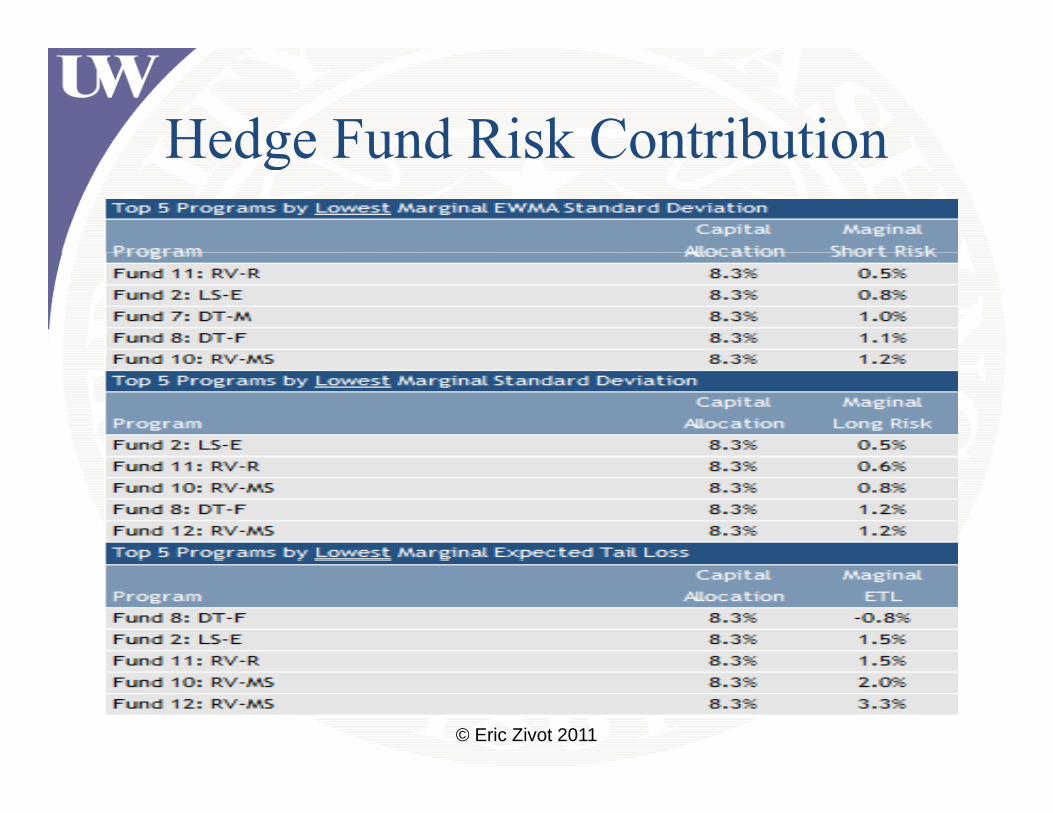
Hedge Fund Risk ContributionHedge Fund Risk Contribution
© Eric Zivot 2011

Summary and ConclusionsSummary and Conclusions
• Factor models are widely used in academicFactor models are widely used in academic research and industry practice and are well suited to modeling asset returnssuited to modeling asset returns
• Tail risk measurement and management of portfolios poses unique challenges that can beportfolios poses unique challenges that can be overcome using Factor Model Monte Carlo methodsmethods
© Eric Zivot 2011
Recommended


![[PPT]PowerPoint Presentation - amcknight / FrontPageamcknight.pbworks.com/w/file/fetch/69919068/Scale Factor... · Web viewScale factor = new measurement old measurement Scale factor](https://img.dokumen.tips/doc/110x75/5af654497f8b9a92719015f2/pptpowerpoint-presentation-amcknight-factorweb-viewscale-factor-new-measurement.jpg)