Extended t-J model – the variational approach
T. K. Lee
Institute of Physics, Academia Sinica, Taipei, Taiwan
July 10, 2007, KITPC, Beijing

Outline• Background and motivation
• Variational Monte Carlo method -- basic approach -- improve trial wave functions increase variational parameters power Lanczos method
• Hole-doped cases, antiferromagnetic (AFM) and superconducting states.
-- ground state -- excitations
• Electron-doped cases
• Summary

Damscelli, Hussain, and Shen, Rev. Mod. Phys. 2003
Phase diagram
holeelectron

Phase diagram
Only AFM insulator (AFMI)? How about metal (AFMM), if no disorder?
Coexistence ofAF and SC?
Related to the mechanism of SC?

H Mukuda et al., PRL (’06)
Phase diagram for multi-layer systemsUD Hg-1245
(Tc=72K, TN~290K)
AFM (0.69μB)
AFM (0.67μB)
AFM (0.67μB)
AFM (0.69μB)
AFM (0.67μB)
AFM (0.67μB)
SC(72K)
+AFM(0.1μB)
SC(72K)
+AFM(0.1μB)
SC(72K)
+AFM(0.1μB)
SC(72K)
+AFM(0.1μB)

“ideal” Phase diagram for hole-doped cupartes?

H. Mukuda et al., PRL 96, 087001 (2006).

Kitaoka, Mukuda et al. PRL (‘06)
Zero-field NMR spectrum at 1.4K
Coexisting state of SC and AFM is realized on a single CuO2 plane (OP) !!
Nh(IP)~0.06, Nh(OP)=0.22
Nh(IP)~0 , Nh(OP)~0.08?
Nh(IP)~0.08? , Nh(OP)=0.24
AFMM

15.20 15.22 15.24 15.26 15.28
H//coriented powder
Hg- 1245 f=174.2MHzT=280K
Inte
nsi
ty (
a.u
.)
H (T)
OP IP+ IP*
Linewidth 50 Oe (IP)
Flatness of CuO2 plane
150 Oe
50 Oe
Narrowest among high-Tc cuprates !
・ Ideal flatness
・ Hole is homogeneously doped
Slide From H. Mukuda

Basic info from experiments
• 5 possible phases: AFMI, AFMM, d-wave SC, and AFM+d-SC, normal
metal. e-doped system is different from hole-doped. Broken symmetries: particle and hole; AFM, SC…
Theoretical challenge:the simplest model to account for all these properties?
To start, only consider the homogeneous solution.

Minimal theoretical models
• 2D Hubbard model – U and t differ by almost an order of magnitude, reliable numerical approaches:
exact diagonalization (ED) for 18 sites with 2 holes (Becca et al, PRB 2000)
finite temp. quantum Monte Carlo (QMC) , fermion sign problem ( Bulut, Adv. in Phys. 2002)
2D t-J type models –

Three species: an up spin, a down spin or an empty site or a “hole”
Model proposed by P.W. Anderson in 1987:t-J model on a two-dimensional square lattice, generalized toinclude long range hopping
jijiji
jijiij nnssJCHcctH
,, 4
1..
iii ccn
Constraint: For hole-doped systemstwo electrons are not allowed on the same lattice site
tij = t for nearest neighbor charge hopping,
t’ for 2nd neighbors, t’’ for 3rd , t’ and t’’ breaks the particle-hole symmetryJ is for n.n. AF spin-spin interaction
,21spinsi

Minimal theoretical models
• 2D Hubbard model – U and t differ by almost an order of magnitude, reliable numerical approaches
exact diagonalization (ED) for 18 sites with 2 holes (Becca et al, PRB 2000)
finite temp. quantum Monte Carlo (QMC) , fermion sign problem ( Bulut, Adv. in Phys. 2002)
2D t-J type models –
no finite temp. QMC – sign problem and strong constraint
ED for 32 sites with 1,2 and 4 holes (Leung, PRB)

Variational Monte Carlo method
Expectation values of an operator O in |>:
Bases:
-- the probability of config. α
Metropolis algorithmSlater determinant

After a series of configurations (1,2,…,M) is generated, expectation values of the operator O is given by
with error
To estimate the accuracy of <O>, Do MG independent Monte-Carlo runs with different initial configurations.
with error
Here, M total number of configurations! Is it accurate?
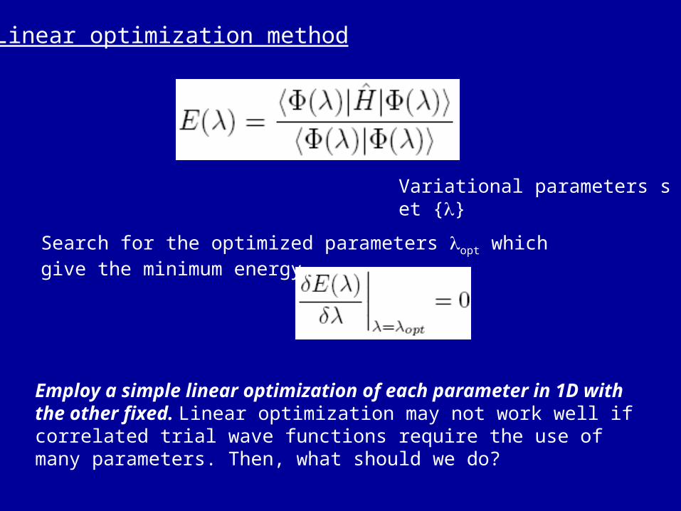
Linear optimization method
Variational parameters set {}
Search for the optimized parameters opt which give the minimum energy,
Employ a simple linear optimization of each parameter in 1D with the other fixed. Linear optimization may not work well if correlated trial wave functions require the use of many parameters. Then, what should we do?

Stochastic reconfiguration (SR) method
Optimization for variational energy:
By Taylor expansion of for ,
pi: variational parameters, i=1,2,…,vp.: a given configuration {R1,…,RN}
, where the Oi operator is
Up to O(pi2)
First,
Casula, et. al., J. Chem. Phys. ’04Sorella, PRB ’05Yunoki and Sorella, PRB ‘06

Similar to steepest descent (SD) method, we define a “force”:
The energy improvement is approximately written as
Energy will converge to the minimum when all Fi=0.We can tune t(>0) to control the convergence of iteration.
We can obtain the next parameters pi’ by iterating
Similar to steepest descent (SD) method, we define a “force”:

However, SD method overlooks a possibility that a small pi may lead to a large change of the wave function…
Therefore, we also need to minimize a “distance”:
we ignore O(pi3) terms
A functional is defined as
is a Lagrange multiplier

Minimization of f(pi) with respect to pi, we have a “new” iterated formula:
t=1/2
Then, the energy improvement for SR method becomes
Sij matrix remains positive definite.
Sometimes Sij has no inverse matrix for some unstable iterations. If so, we use the SD method instead.

How do we choose t in SR method?
2D Lattice size=64t-t’-t’’-J model with (t’,t’’,J)=(-0.3,0.2,0.3) Trial wave function: d-wave RVB wave functionn is the number of iterations
linear
SR

For a given trial wave function, , we approach the ground statein two steps:
1. Lanczos iteration
||| 1)1( HN
C
|||| 2221)2( HH
N
C
N
C
C1 and C2 are taken as variational parameters
)()( |)(| lnln W H
2. Power Method
)()( |)(|| lim lnln W
nGS H
Beyond VMC approach – the Power-Lanczos method
|
We denote this state as |PL1>
|PL2>

J=0.3 E
Exact -0.583813
RVB(PL0) -0.5431
RVB(PL1) -0.5654
RVB(PL2) -0.5709
PL Energy
After PL, nk, HH(R), and energy get closer to exact results!
For the t-J model, LeungPRB 2006, 4 holes in 32 sites

HH(R) – the hole-hole correlation function

Trial wave functions for hole-doped systems
Must account for : Mott insulatorAFM, SC , AFM+SC?

This provides the pairing mechanism! It can be easily shown that near half-filling this term only favors d-wave pairing for 2D Fermi surface!
jiji
ji
jijijiji
ji
jijijiJ
J
CCCCCCCCJ
nnssJH
,,
,
,,,,,,,
,,
,
2
))((2
4
1
In 1987, Anderson pointed out the superexchange term
Spin or charge pairing?
jijiji
jijiij nnssJCHcctH
,, 4
1..
AFM is natural!D-wave SC?

The resonating-valence-bond (RVB) variational wave function pr
oposed by Anderson ( originally for s-wave and no t’, t’’),
BCSCCvuRVB kk
kkk d,,d P0)(P
)1(Pd ii
inn
d-RVB = A projected d-wave BCS state!
The Gutzwiller operator Pd enforces no dou
bly occupied sites for hole-doped systems
AFM was not considered.
2 2
/ , (cos cos )
2(cos cos ) 4 ' cos cos 2 '' (cos 2 cos 2 ) ,
k kk k k v x y
k
k x y v x y v x y v
k k k
Ev u k k
k k t k k t k k
E
four variational parameters, tv’ tv’’ ∆v, and μv

The simplest way to include AFM:
RVB))1(*exp( iz
i
itr Sh
Lee and Feng, PRB 1988, for t-J

Assume AFM order parameters:
zB
zA ssm staggered magnetization
ji ccAnd uniform bond order
jiji
cccc
yjiif
xjiif
ˆ,
ˆ,
Use mean field theory to include AFM,
Two sublattices and two bands – upper and lower spin-density-wave (SDW) bands
Lee and Feng, PRB38, 1988; Chen, et al., PRB42, 1990; Giamarchi and Lhuillier, PRB
43, 1991; Lee and Shih, PRB55, 1997; Himeda and Ogata, PRB60, 1999

RVB + AFM for the half-filled ground state (no t, t’ and t’’)
0 02
/
Ne
kkkkkkk bbBaaA
k
kkk
EA
Pd
k
kkk
EB
iiid nnP 1
&
Ne= # of sites
Variational results
)1(3324.0 ji ss
staggered moment m = 0.367
“best” results
-0.3344
0.375 ~ 0.3
Liang, Doucot
And Anderson
bandsSDWupperbSDWlowera kk &
21
22kkkE 2
1222
43 coscos JmkkJ yxk

The wave function for adding holes or removing electrons from the half-filled RVB+AFM ground state
A down spin with momentum –k ( & – k + (π, π ) ) is removed from the half-filled ground state. --- This is different from all previous wave functions studied.
Lee and Shih, PRB55, 5983(1997); Lee et al., PRL 90 (2003); Lee et al. PRL 91 (2003).
0P
)2/1,(
12/
d
01
Ne
kqqqqqqqk
kzh
bbBaaAc
cSk The state with one hole (two parameters: mv and Δv)Creating charge excitations to the Mott Insulator “vacuum”.

Dispersion for a single hole. t’/t= - 0.3, t”/t= 0.2
The same wave function is used for both e-doped and hole-doped cases.
There is no information about t’ and t” in the wave function used.
Energy dispersion after one electron is doped. The minimum is at (π, 0). t’/t= 0.3, t”/t= - 0.2
J/t=0.3
1st e-
1st h+
□ Kim et. al. , PRL80, 4245 (1998); ○ Wells et. al.. PRL74, 964(1995); ∆ LaRosa et. al. PRB56, R525(1997).● SCBA for t-t’-t’’-J model, Tohyama and Maekawa, SC Sci. Tech. 13, R17 (2000)

ARPES for Ca2CuO2Cl2
The lowest energy at
)2/,2/( k
Ronning, Kim and Shen, PRB67 (2003)
Nd2-xCex CuO4 -- with 4% extra electrons
Fermi surface around (π,0)and (0, π)!
Armitage et al., PRL (2002)

)2/1),2/,2/((1 zh Sk Momentum distribution for a single hole calc. by the quasi-particle wave function
< nhk↑> < nh
k↓ >
Exact resultsfor the single-hole ground statefor 32 sites.Chernyshev et al.PRB58, 13594(98’)
64 sites

Wave Functions for one hole system
• Quasi-particle state:
0)(1
2'
N
kqqqqqqakd bbBaaACP
Hole momentum (kh)=unpaired spin momentum (ks) = k
0)(1
2'
N
kqqqqqqakd
h
sbbBaaACP
)2
,2
(
hs kkwhere ,
• Spin-bag state:

a QP state kh=(,0) = ks a SB state ks =(,0), kh=(/2, /2)
Exact 32 site result from P. W. Leung for the lowest energy (π,0) state t-J t-t’-t’’-J

Takami TOHYAMA et al.,
J. Phys. Soc. Jpn. Vol 69, No1, pp. 9-12
(0,0)
QP
(0,0)
SB
(/2,/2)
QP
(,0)
QP
(,0)
SB
a 0.188 -0.0288 -0.0044 0.123 -0.0313
b 0.188 -0.0254 -0.0052 0.159 -0.0085
c 0.202 -0.0302 -0.0005 0.071 -0.002
d -0.273 -0.203 -0.2241 -0.353 -0.1921
e -0.264 -0.195 -0.2154 -0.279 -0.2115
Our Result: (π, 0) is QP at t-J model, but SB for t-t’-t”-J.
(0, 0) is QP for both
QP:Quasi-Particle state
SB: Spin-Bag state
J/t=0.4, t’/t-α/3 and t”/t’=2/3

0P
)0,0(
12/
d
02
Ne
kqqqqqqq
kkZtotalh
h
hh
bbBaaA
ccSk Ground state is kh=(π/2, π/2)for two 0e holes; kh=(π,0) for two 2e holes.
The state with two holes
Similar construction for more holes and more electrons.
The Mott insulator at half-filling is considered as the vacuum state.Thus hole- and electron-doped states are considered as thenegative and positive charge excitations .
Fermi surface becomes pockets in the k-space!
Lee et al., PRL 90 (2003); Lee et al. PRL 91 (2003).

The new wave function has AFM but negligible pairing.It could be used to represent an AFM metallic (AFMM) phase.
d-wave pairing correlation function
2 holes in 144 sites

2 holes in 144 sites

Increase doping, pockets are connected to form a Fermi surface:
Cooper pairs formed by SDW quasiparticles
three new variational parameters: μv, t’v and t”v

AFMM shows stronger hole-hole repulsive correlation than AFMM+SC.
The pair-pair correlation of AFMM is much smaller than AFMM+SC.

μv, t’v and t”vmv and Δv
mv and Δv
Δv, μv, t’v and t”v
2k
2kkyxyxyxk
yxkk
kk
k
kk
+=E,)k2cos+k2(cost ′′2kcoskcost′4)kcos+k(cos2=
)kcosk(cos=,E
=u
v=A
Δξμξ
ΔΔΔ
ξ
----
--
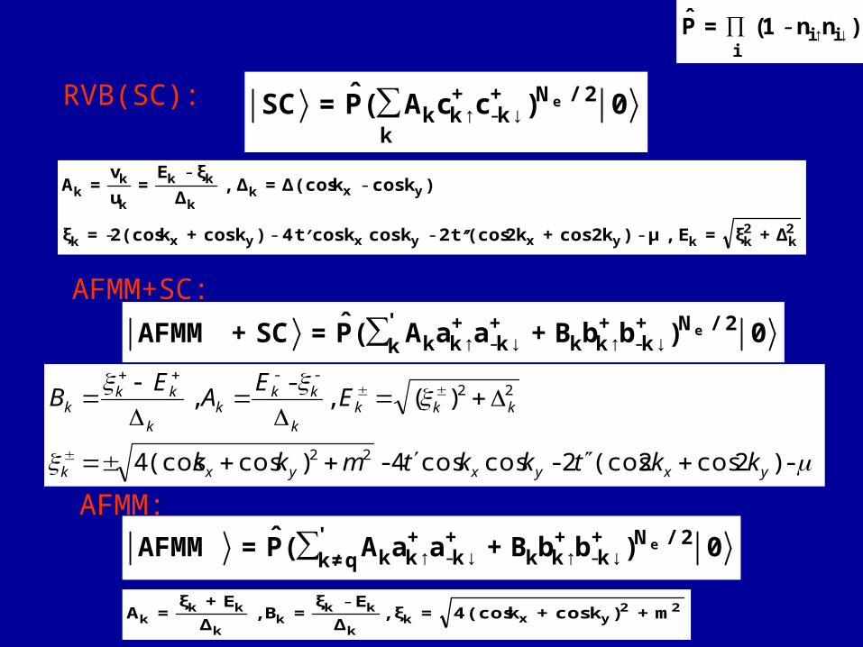
All trial wave functions:
RVB(SC): 0)ccA(P̂=SC 2/N
k
+k
+kk
e∑ ↓-↑
)nn1(=P̂ iii
↓↑-∏
AFMM+SC:
0)bbB+aaA(P̂=SC+AFMM 2/N'k
+k
+kk
+k
+kk
e∑ ↓-↑↓-↑
-)2cos2(cos2-coscos4-)cos(cos4
)(,-
,
22
22--
yxyxyxk
kkkk
kkk
k
kkk
kktkktmkk
EE
AE
B
AFMM:0)bbB+aaA(P̂=AFMM 2/N'
q≠k+k
+kk
+k
+kk
e∑ ↓-↑↓-↑
22yxk
k
kkk
k
kkk m+)kcos+k(cos4=,
E=B,
E+=A ξ
Δ
ξ
Δ
ξ -

Variational Energy
Phase diagram

SDW: 0)aaA(P̂=SDW 2/N'k
+k
+kk
e∑ ↓-↑
)(=A kk--ξΘ bandsSDWupperb;SDWlowera kk : : σσ
The energy difference among these states

CT Shih et al., LTP (’05) and PRB (‘04)t’/t=0 t’’/t=0
t’/t=-0.3, t’’/t=0.2
AFMM+SC
AFMM
x0.60.50.40.30.20.1
Possible Phase Diagrams for the t-J model
t’/t=-0.2t’’/t=0.1

Phase diagram for hole-doped systems
H Mukuda et al., PRL (’06)
The “ideal” Cu-O plane
Extended t-J model, t’/t=-0.2, t’’/t=0.1
Summary – I • Variational approach provides a quantitative way to unde
rstand the t-J or extended t-J model by taking into account the projection rigorously.
• Based on the RVB concept, trial wave functions for the doped system have been constructed to represent the AFMM, AFMM+SC and SC phases observed in multilayer cuprates.
• With the values of t, t’ and J in the range of experiments, the phase diagram obtained agree with cuprates below optimal doping.

Acknowledgement
• Y. C. Chen, Tung Hai University, Taichung, Taiwan• R. Eder, Forschungszentrum, Karlsruhe, Germany • C. M. Ho, Tamkang University, Taipei, Taiwan• C. Y. Mou, National Tsinghua University, Taiwan• Naoto Nagaosa, University of Tokyo, Japan• C. T. Shih, Tung Hai University, Taichung, TaiwanStudents:• Chung Ping Chou, National Tsinghua University, Taiwan• Wei Cheng Lee, UT Austin• Hsing Ming Huang, National Tsinghua University, Taiwan

Outline• Background and motivation
• Variational Monte Carlo method -- basic approach -- improve trial wave functions increasing variational parameters power Lanczos method
• Hole-doped cases, antiferromagnetic (AFM) and superconducting states.
-- ground state -- excitations
• Electron-doped cases
• Summary

Excitations in the SC state
)cos(cos,/ yxqq
qqqqq qq
Euva
With a fixed-number of holes, the d-RVB state becomes
The ground state 0)(P,,d'
k
kkkkt
CCvuRVB
0)(P,1 2/,,,d
q
Nqqqke
eCCaCkN
)( 22kkkE
Quasi-particle excitation
Excitation energies are fitted with

0)(P,1 2/,,,d
q
Nqqqke
eCCaCkN
)( 22kkkE Excitation energies are fitted with
Example:
QP excitation
t’/t, t’’/t, and /t are renormalized and “Fermi surface” is determined by Setting =0 in the excitation energy.

J/t=0.3, t=0.3eV t’/t=-0.3 & t’’/t=0.2 for YBCO and BSCO
but t’/t=-0.1 & t’’/t=0.05 for LSCO
Our VMC overestimates the gap by a factor of 2, PRB 2006

Anomalies in the spectral weight for the low-lying excitations.
For Gutzwiller-projected wave functions??
For ideal Fermi gas : 0
kk n1Z 0
kk nZ
For BCS theory : 2
kk uZ 2kk vZ
mmk
mmk EECmEECmkA 0
2
,0
2
, 00),(

Exact Identity :
S. Yunoki, cond-mat/0508015, C.P. Nave et al., cond-mat/0510001
No exact relation is known about
Using the identities,

Is this relation between pairing amplitude and spectral weight also true for projected wave functions?
BCS theory predicts
2k
2k
2kkk vuZZ
So what is ?
YES!!

Pairing amplitude by VMC (II):
C.T. Shih et al., PRL
Long-range pair-pair correlation

Anomalies in STS conductance
S.H. Pan et al., unpublished data
OPD
T. Hanaguri et al., Nature
Ca2-xNaxCuO2Cl2
MgB2

McElroy et al. Science (05)

Could the asymmetry be DOS effects ?
d-BCS with 2 bands
B. W. Hoogenboom et al. PRB (‘03)
as hole doped
d-wave gap opened !
DOS singularity
Hoffman
M. Cheng et al. PRB (‘05)

Particle-hole asymmetry for STS conductance
2
, 0 00k m k km k
m C E E Z E E
0k kk
Z E E
the tunneling conductance at negative bias:
For positive bias:
mmk
mmk EECmEECmkA 0
2
,0
2
, 00),(
Conductance is related to the spectral weight

Quasi-particle contribution to the conductance ratio
d-RVB (t’=-0.3, t’’=0.2)
d-BCS
E=0.3t for 12X12E=0.2t for 20X20

Quasi-particle contribution to the conductance ratio :
d-RVB (t’=-0.3, t’’=0.2)
d-BCS

Spectral weight PEAK HEIGHTS and GAP SIZES

Why is d-wave SC so robust?
McElroy et al. Science (05)

Consider the impurity elastic scattering matrix element
, ' , ', 'k k k kV k C C k
For BCS theory, this is just uk u k’ – vk v k’
0)(P,1 2/,,,d
q
Nqqqke
eCCaCkN
But for projected states, there is a strong renormalization
, ' , ',1, 1, 'k k e k k eV N k C C N k

, ' , ',1, 1, 'k k e k k eV N k C C N k
0)(P,1 2/,,,d
q
Nqqqke
eCCaCkN
gt=2x/(1+x) RenormalizedMean-fieldtheory ,Garg et al,Cond-mat/0609666
15 holes in 12*12

Summary - II
• In addition to studying ground states, variational approach could also study excitation spectra, STM conductance asymmetry, effects of disorder (why d-wave is so robust) etc..

Hole-doped Electron-doped
T’ phaseT phase
Electron-doped systems

Damscelli, Shen and Hussain, Rev. Mod. Phys. 2003
Phase diagram:

jijiji
jijiij nnssJCHcctH
,, 4
1..
t for n.n., t’ for 2nd n.n., and t” for 3rd n.n.
Consider t-t’-t”-J model:
For electron-doped, no empty sites!! “Lower Hubbard band is projected out”

Experiments M. Ikeda,
thesis ‘06
T. Kubo, Physica C ‘02

VMC
(0.1,-0.05)
(t’,t’’)
(0.15,-0.1)
(0.3,-0.2)

Recent ARPES for Nd2-
xCexCuO4:
16.5 eV --- Armitage et al., PRL 2002
55 eV --- Armitage et al., PRL 2001
(x=0.15)
400 eV --- Claesson et al., PRL 2004
(x=0.15)
22 eV --- H. Matsui et al., 0410388
(x=0.13)

NCCO
SCCO
Non-uniform gap!(x=0.13, TN=110K, T=30K)
x=0.14, Tc=13K,T~18K, TN=110K

• A gap near (π,0) region, but not near (π/2,π/2)• The gap increases as it moves away from (π,0)• The “lower” band approaches Fermi energy near (π /2, π /2) and the peaks are broad• Could these be lower and upper SDW bands??
Near (π,0) Near (π/2,π/2)

t-J model only has the upper Hubbard band
+
“AF LRO”
k and k + Q are coupled!!Q= (π,π)
In weak coupling analogy, 2 “SDW” bands

zB
zA ssm staggered magnetization:
ji ccuniform bond order:
jiji cccc
yjiif
xjiif
ˆ,
ˆ,
d-wave RVB pairing:
2 sublattices and 2 bands – upper and lower SDW bands
G.J. Chen at al. 1990, Giamarchi and Lhuiller, 1991
Same asa
same as the hole-doped case

..
,,
CHbbaa
bbaaH
kkkkkk
kkkk
kkkkMF
bandsSDWupperbSDWlowera kk &
21
222
43 coscos JmkkJ yxk
yxk kkJ coscos43
Mean-field Hamiltonian for lower and upper SDW bands:
with

A down spin with –k (–k+Q) is removed from the half-filled ground state.
Dope one hole
Create charge excitations in the Mott Insulator “vacuum”,The AFMM state:
Dope one electron
0bbBaaA'C P
C)2/1S,k(
12
N
kqqqqqqqkd
0kzh1
0bbBaaA'CCC P
C)2/1S,k(
12
N
kqqqqqqqQkQkkd
0kze1
T. K. Lee, et al., PRB 1997; T. K. Lee, et al., PRL 2003; W. C. Lee, et al., PRL 2003.
all quantities could be calculated with hole wf except t’/t → – t’/t and t”/t → – t”/t

0)(P
)2/1,(
12'
d
01
N
kqqqqqqqkQkQk
kze
bbBaaACCC
cSk
1 electron wave function:
Another similar wave function:
0)(P
)2/1,(
12'
d
01
N
kqqqqqqqkkQk
Qkze
bbBaaACCC
cSQk
These 2 wave functions have a finite overlap!

(0,0) (π,0) (π,π) (0,0)
Fermi level
2 occupied states for the same k
0bbBaaA'
CCCC P)2/1S(
102
N
region ,0)(qqqqqqq
10
region ,0)(kQkQkkkdze20
Consider 20 doped electrons in 144 sites:

or Outside (π,0) region
(0,0) (π ,0) (π,π) (0,0)
Fermi level
Remove an electron from this (π,0) region
(0,0) (π ,0) (π,π) (0,0)
Fermi level
(1)
(2)

0bbBaaA'
CCCC P)2/1S(
102
N
region ,0)(qqqqqqq
10
region ,0)(kQkQkkkdze20
Consider 19 doped electrons in 144 sites:
another similar wave function: )2/1,(19 ze SQk
QP state
0bbBaaA'
CCCCCCC P)2/1S,k(
102
N
k & region ,0)(qqqqqqq
9
region ,0)(kQkQkkkQkQkkdze19
0bbBaaA'
CCCCC P)2/1S,k(
112
N
k & region ,0)(qqqqqqq
10
region ,0)(kQkQkkkkdze19
(1)
(2)

Spectral Weight
(π,0) (5π/6,π/6) (2π/3,π/3) (π/2,π/2)
USDW (19e) 3.23E-01 2.99E-01 2.08E-06 8.61E-08
USDW (27e) 3.08E-01 3.00E-01 9.76E-06 8.31E-08
LSDW (19e) 5.63E-02 7.51E-02 1.41E-02 1.29E-02
LSDW (27e) 1.08E-01 1.12E-01 2.07E-02 1.90E-02
12 by 12, x=013 & 0.19
16 by 16, x=0.17
Gap exists only near (π,0)!Gap is K-dependent!


Conclusions:
• The e-doped t-t’-t’’-J model has been studied in the low energy states.
• At low doping, small FS pockets appear around anti-nodal points.
• Upon increased doping, AF will become weaker.• Based on the AFMM states and coupling between k and k
+ Q= (π,π), the evolution of the FS with doping and the calculated spectral weight are in good qualitative agreement with the ARPES data.
• Questions remained: The doping dependence of phase diagram? Other excited states to be considered? SC+AFM coexistent state ?
Thank you for your attention!
Recommended