Download pdf - Evolution of the Leading-Edge Vortex over an Accelerating ... · PDF file234 Yossef Elimelech et al. / Procedia IUTAM 7 ( 2013 ) 233 – 242 Nomenclature c¯ mid-span chord length

Procedia IUTAM 7 ( 2013 ) 233 – 242

2210-9838 © 2013 The Authors. Published by Elsevier B.V.Selection and/or peer-review under responsibility of the Isaac Newton Institute for Mathematical Sciences, University of Cambridgedoi: 10.1016/j.piutam.2013.03.027

Topological Fluid Dynamics: Theory and Applications

Evolution of the leading-edge vortex over an accelerating rotatingwing

Yossef Elimelecha ∗, Dmitry Kolomenskiyb, Stuart B. Dalzielc, H. K. Moffattc

aFaculty of Aerospace Engineering, Technion-Israel Institute of Technology, Haifa 32000, IsraelbCentre Europeen de Recherche et de Formation Avancee en Calcul Scientifique, 42 avenue Gaspard Coriolis, 31057 Toulouse Cedex 01, FrancecDepartment of Applied Mathematics and Theoretical Physics, Centre for Mathematical Sciences, University of Cambridge, Wilberforce Road,

Cambridge CB3 0WA, United Kingdom

Abstract

The flow field over an accelerating rotating wing model at Reynolds numbers Re ranging from 250 to 2000 is investigated using

particle image velocimetry, and compared with the flow obtained by three-dimensional time-dependent Navier-Stokes simulations.

It is shown that the coherent leading-edge vortex that characterises the flow field at Re∼200-300 transforms to a laminar separation

bubble as Re is increased. It is further shown that the ratio of the instantaneous circulation of the leading-edge vortex in the accel-

eration phase to that over a wing rotating steadily at the same Re decreases monotonically with increasing Re. We conclude that

the traditional approach based on steady wing rotation is inadequate for the prediction of the aerodynamic performance of flapping

wings at Re above about 1000.

c© 2012 Published by Elsevier Ltd. Selection and/or peer-review under responsibility of K. Bajer, Y. Kimura, & H.K. Moffatt.

Keywords: flapping flight; unsteady aerodynamics; leading-edge vortex evolution; particle image velocimetry; Navier-Stokes simulations

∗ Corresponding author

E-mail address: [email protected]

Available online at www.sciencedirect.com

© 2013 The Authors. Published by Elsevier B.V.Selection and/or peer-review under responsibility of the Isaac Newton Institute for Mathematical Sciences, University of Cambridge

234 Yossef Elimelech et al. / Procedia IUTAM 7 ( 2013 ) 233 – 242

Nomenclature

c mid-span chord length

R wing span

X dimensional coordinate in the streamwise direction (wing frame of reference)

Y dimensional coordinate parallel to the axis of rotation

Z dimensional spanwise coordinate in the wing frame of reference

x dimensionless coordinate in the streamwise direction (wing frame of reference), x = X/cy dimensionless coordinate parallel to the axis of rotation, y = Y/cz dimensionless spanwise coordinate in the wing frame of reference, z = Z/Rt time from start of stroke motion

τ time constant

U dimensional flow velocity components in the wing frame of reference

u dimensionless flow velocity components in the wing frame of reference, u = U/(z Rθ)uz dimensionless spanwise velocity component

θ angular location from start of stroke motion

θ∞ angular velocity of wing in steady rotation

α geometric angle-of-attack

ν fluid kinematic viscosity

Re Reynolds number, Re=θ∞Rc/νωz dimensional spanwise vorticity

ωz dimensionless spanwise vorticity, ωz = ωz c/(zRθ)Γ circulation

Σ symmetric part of velocity gradient tensor

Ω antisymmetric part of velocity gradient tensor

1. Introduction

Flapping flight has been a subject of interest for several centuries since the visionary ideas of Roger Bacon and

Leonardo da Vinci. Since Weis-Fogh’s [1] analysis of hovering animal flight, many authors have studied flow mecha-

nisms of hovering insects, and our understanding of insect flight mechanisms has advanced significantly over the last

two decades through many experimental and numerical explorations. Most studies fall into two main groups: the first

analyses the flow over periodically flapping wings; the second analyses the flow over rotating wings like propellers,

simulating the mid-stroke of the flapping cycle but not the wing rotation at the end of each cycle.

For insects, it is generally accepted that most of the lift is associated with a large, stable leading-edge vortex (LEV)

which separates from the sharp leading edge of the wing [2]. Other features of this leading-edge vortex, such as its

spanwise distribution [3, 4] or its stability [5, 6], are more controversial. Usherwood & Ellington [7] showed that

the LEV is stable on a steadily rotating wing like a propeller. The resultant aerodynamic force is normal to the wing

surface, reflecting the fact that the LEV essentially eliminates the leading-edge suction. The practical consequence of

this result is a low lift-to-drag ratio; the high vertical force coefficients measured in propeller tests for various aspect

ratios and Reynolds numbers Re were therefore inevitably associated with high aerodynamic drag.

An important aspect of hovering flight which cannot be treated using steadily rotating wings is the lift evolution

after the abrupt wing rotation (about the wing axis) which occurs at either end of the wing stroke. During each end-

of-stroke rotation, the existing LEV separates from the wing surface and a ‘newly born’ LEV is formed once the wing

starts to accelerate through the following wing stroke. It is important to determine the time-scale of development of

the new LEV as this is directly related to the time it takes for the aerodynamic lift (and drag) to reach its ultimate

value. While optimistic estimates assume immediate formation of the LEV, more realistic evaluations are needed to

better understand the detailed flow mechanisms of hovering flight.

A recent study [8] discussed the time evolution of the flow field over a dynamically-scaled flapping wing at Re =


250 and angle-of-attack α = 50o. It is believed that such a high angle-of-attack is unlikely to be representative of

insect flight; we therefore initiated the present study with an experiment at Re = 250 and α = 30o.

Micro air vehicles are currently designed for Reynolds numbers that are higher than this by an order of magnitude

or more, yet little is known about the nature of the transient flow field over flapping wings in this regime. The present

experimental study discusses the evolution of the flow field and the formation of the leading-edge vortex over an

accelerating rotating wing up to Re = 2000. We observed a coherent LEV at Re = 250; a separation bubble bounded

by a sheet of vorticity shed from the leading edge at Re = 1000; and an instability of this vortex sheet at Re = 2000.

We focus on the first quarter of the wing flapping cycle, i.e. half of the stroke of a flapping wing. The flow field during

this acceleration phase is compared to the flow that develops over a steadily rotating wing in order to highlight the

differences between the two. We find that at the end of the first quarter of a cycle, the circulation around the wing

exceeds its steady-state value at Re = 250, but that at Re = 1000 it remains below the corresponding steady-state

value. Later, we discuss the question, important for engineering applications, as to whether the flapping-wing strategy

is aerodynamically advantageous at Reynolds numbers above 250 as compared with steady wing rotation.

2. Setup and methods

2.1. Experimental setup

The study was performed using a controlled wing suspended in a Perspex tank (400×400×500 mm) filled with

water-glycerin solution of kinematic viscosity ν = 3.92 · 10−6(±6%) m2/s (Fig. 1a and c). A real-time control unit

(National Instruments cRIO-9022 controller together with the NI-9505 DC brushed servo module) controlled a servo

motor which rotated the wing around a vertical axis. The wing’s planform was a triangle machined from a 1.5 mm

thick stainless steel flat plate. The distance between the centre of rotation and the wing tip (i.e. the wing length) was

R=100 mm and the tip chord length was 50 mm (Fig. 1b).

The flow field was obtained using two-dimensional particle image velocimetry . Data was acquired at five equidis-

tant span locations between Z/R = 0.4 and Z/R = 0.8 (see Fig. 1b), where Z is the coordinate along the span. Using

a high frame-rate digital camera (Photron FASTCAM-ultima APX 120K, 1000 by 1000 pixel resolution) and a Nikon

60 mm f/2.8G ED AF-S Micro NIKKOR lens, a field of view of approximately 60 by 60 mm was recorded. This

allowed capturing the flow over the entire chord at all span locations and some of the flow details of the near wake.

Silver-coated hollowed glass spheres with a mean diameter of 10 μm (Dantec Dynamics Ltd.) were used as seeding

particles. The flow was illuminated by a high repetition dual cavity Nd:YLF laser head (10 mJ/pulse per cavity at 527

nm). A cylindrical lens (f = 7.8 mm) was used to create a thin light sheet approximately 2 mm thick; the light sheet

illuminated several span stations, as shown in Fig. 1b.

During the wing motion, high frame-rate image sequences were recorded at several angular wing positions, namely,

θ=10, 22.5, 45, 67.5 and 90o, from the start of the motion. Using information from the servo motor encoder, a

synchronisation pulse was fired to the camera and the laser head at these specific angular locations. In order to

keep the same camera calibration and illumination settings, the initial angular position of the wing was modified to

allow image capturing at a fixed location with respect to the camera. For better signal-to-noise ratio, each case was

repeated 20 times. At the end of each wing stroke the wing decelerated to rest, and a pause of approximately 60s

was inserted between two successive wing strokes to establish an essentially quiescent flow at the beginning of each

stroke. The PIV processing was conducted using DigiFlow [9]. For each PIV plane, two in-plane velocity components

were computed from the cross-correlation of pairs of successive images with 50% overlap between the interrogation

domains. The high seeding density allowed high quality vector fields for interrogation windows of 21 by 21 pixels.

2.2. Numerical setup

Rigid wings moving in an incompressible viscous fluid are considered, as described in [10]. The no-slip boundary

condition at the solid boundary is modelled using the volume penalisation method [11] . The penalised Navier-

Stokes equations are solved using a classical Fourier pseudo-spectral method. The spatial computational domain is a

rectangular box with periodic boundary conditions imposed on all its faces. The computational domain of size Lx ×Ly×Lz = 123 was uniformly discretised with 7683 grid points. The time integration is exact for the viscous term and


Fig. 1. Experimental setup: (a) general illustration showing the tank, the rotating wing and the camera-illumination setup; (b) top view of the

wing-shaft assembly showing the wing planform, the rotation angle and the planes where images were obtained; (c) side view of the wing-shaft

assembly showing the geometric angle-of-attack with respect to the horizon.

an adaptive second-order Adams-Bashforth scheme is used for the nonlinear term [12]. The parallel implementation

of the code employs the P3DFFT fast Fourier transform package.

2.3. Kinematics

In order to parameterise the complex motion of a flapping wing, the wing kinematics was simplified to an angular

motion at a constant geometric angle-of-attack of 30o (Fig. 1c). Starting from rest, the wing followed the kinematic

relation θ/θ∞ = (1− e−t/τ ), where θ is the wing rotation angle, θ∞ is the ultimate angular velocity of the wing, t is

elapsed time from motion start and τ is a time constant. In order to represent a realistic manoeuvre of a periodically

flapping wing, the motion was subject to the kinematical constraints θ/θ∞(t∗) = 0.99, θ(t∗) = π/2. The Reynolds

number Re= θ∞Rc/ν is based on the maximal tip velocity θ∞R, the mid-span chord of the wing c = R/4, and the

kinematic viscosity ν; in this study, Re ranged from 250 to 2000.

2.4. Flow diagnostics

In order to establish a comparison of the flow field over the wing, the velocity field U, and the spanwise vorticity

component ωz , were referenced to the wing’s instantaneous circumferential velocity at each span. In particular,

the dimensionless velocity components and the spanwise vorticity fields are u = {ux, uy, uz} = U/(z Rθ) and

ωz = ωz c/(zRθ), respectively, where Z is the radial position, R the wing length, c the mid-span chord and z = Z/Rthe dimensionless radial location; using this terminology, the dimensionless spanwise velocity component is denoted

by uz (positive towards the wing tip). Whenever the velocity vector field is shown below, it is given in the wing frame

of reference, not in the inertial frame.

The LEV region was identified using the dimensionless second invariant of the velocity gradient tensor [13]:

E = (‖Σ‖2 − ‖Ω‖2)/(‖Σ‖2 + ‖Ω‖2), (1)

where Σ and Ω are the symmetric and antisymmetric components of the velocity gradient tensor:

Σ =1

2(∇u + (∇u)T ) , Ω =

1

2(∇u − (∇u)T ) . (2)


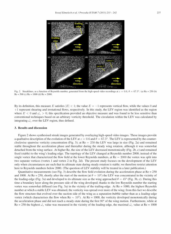
Fig. 2. Streaklines, as a function of Reynolds number, generated from the high-speed video recordings at z = 0.6, θ = 67.5o. (a) Re = 250 (b)

Re = 500 (c) Re = 1000 (d) Re = 2000.

By its definition, this measure E satisfies |E| < 1; the value E = −1 represents vortical flow, while the values 0 and

+1 represent shearing and irrotational flows, respectively. In this study, the LEV region was identified as the region

where E < 0 and ωz > 0; this specification provided an objective measure and was found to be less sensitive than

conventional techniques based on an arbitrary vorticity threshold. The circulation within the LEV was calculated by

integrating ωz over the LEV region, thus defined.

3. Results and discussion

Figure 2 shows synthesised streak images generated by overlaying high-speed video images. These images provide

a qualitative description of the evolution of the LEV at z = 0.6 and θ = 67.5o. The LEV is represented by the counter-

clockwise spanwise vorticity concentration (Fig. 3); at Re = 250 the LEV was large in size (Fig. 2a) and remained

stable throughout the acceleration phase and thereafter during the steady wing rotation, although it was somewhat

detached from the wing surface. At higher Re, the size of the LEV decreased monotonically (Fig. 2b, c) and remained

fixed (stable) to the wing’s leading edge. The topology of the LEV changed at Reynolds number 2000; instead of the

single vortex that characterized the flow field at the lower Reynolds numbers, at Re = 2000 the vortex was split into

two separate vortices (vortex 1 and vortex 2 in Fig. 2d). The present study focuses on the development of the LEV

only when circumstances are such that its ultimate state during steady rotation is stable; we therefore restrict attention

here to Reynolds numbers below 2000. (The question of LEV stability will be treated in a later publication.)

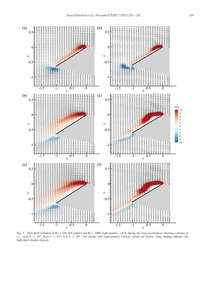
Quantitative measurements (see Fig. 3) describe the flow field evolution during the acceleration phase at Re = 250

and 1000. At Re = 250, shortly after the start of the motion (at θ = 10o) the LEV was concentrated in the vicinity of

the leading-edge (Fig. 3a) and developed to its ultimate size as the wing approached θ = 45o (Fig. 3b, c). During this

time a boundary layer along the pressure side of the wing developed; thanks to the low Reynolds number the starting

vortex was somewhat diffused (see Fig. 3a) in the vicinity of the trailing-edge. At Re = 1000, the highest Reynolds

number at which a stable LEV was obtained, the vorticity was spread over more of the wing; from this fact we describe

the flow structure that evolved over the suction side of the wing as a separation-bubble rather than as a leading-edgevortex (which characterises the flow when Re ∼ 102). At Re = 1000, the vorticity developed monotonically during

the acceleration phase and did not reach a steady-state during the first 90o of the wing motion. Furthermore, while at

Re = 250 the highest ωz value was measured in the vicinity of the leading-edge, the maximal ωz value at Re = 1000


(Fig. 3e, f) was measured in the vicinity of the flow reattachment point. This intense vorticity encouraged induced

reversed velocity which, in turn, created a ’dead-water’ zone inside the separation-bubble; this zone is characterized

by low ωz values near the wing surface and a shear layer above it.

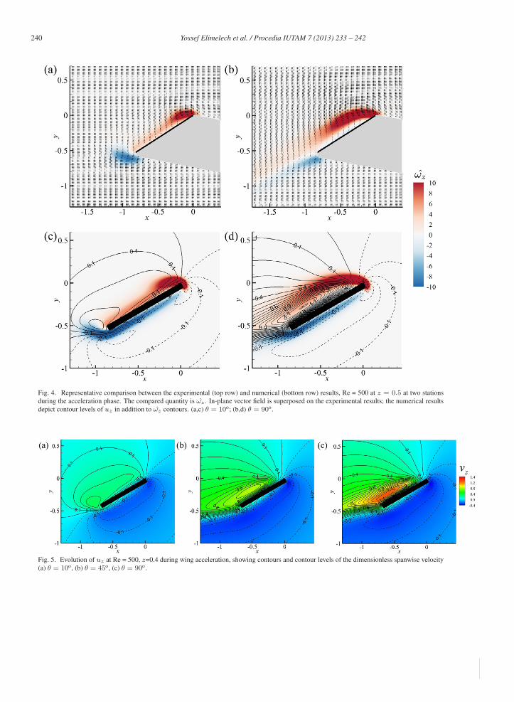
Good agreement between the experimental and numerical results (see representative example in Fig. 4) allowed us

to use the latter to obtain the spanwise velocity component uz , which could not be resolved experimentally using two-

dimensional particle image velocimetry. This spanwise component provides a clear distinction between the flow field

over a rotating wing, and that over a wing in rectilinear motion. A rotating wing experiences a non-uniform spanwise

pressure distribution due to the linearly varying circumferential velocity at each radial location along the wing span.

In such circumstances, the flow field is fully three-dimensional, especially near the root of the wing [6, 14]1. This

phenomenon has already been found to yield high cross-sectional lift coefficients [14]; other studies associated the

augmented lift capacity and postponed stall characteristics with the stability of the LEV which is itself correlated with

uz [6]. In these scenarios, the LEV was found to remain attached along the median portion of the wing while further

out toward the wing tip the LEV lost its coherence and experienced vortex breakdown. As mentioned earlier, we

restrict attention in the present discussion to cases where the LEV was found to remain attached to the wing surface.

We attempted to correlate between the evolution of the spanwise flow and the spanwise vorticity production because

the latter is a direct measure of the aerodynamic load acting on the wing. The evolution of uz during the acceleration

phase is shown in Fig. 5 for Re = 250. As expected, uz increased immediately after the motion began (Fig. 5a). At

z = 0.4 and θ = 10o, uz reached approximately 0.2. Later, when the wing approached θ = 90o (mid-stroke) uz

attained a value as high as 1.2, exceeding the wing’s instantaneous circumferential velocity at that spanwise station

(emphasising the three-dimensional character of the flow). Not only did uz evolve during the acceleration phase, it

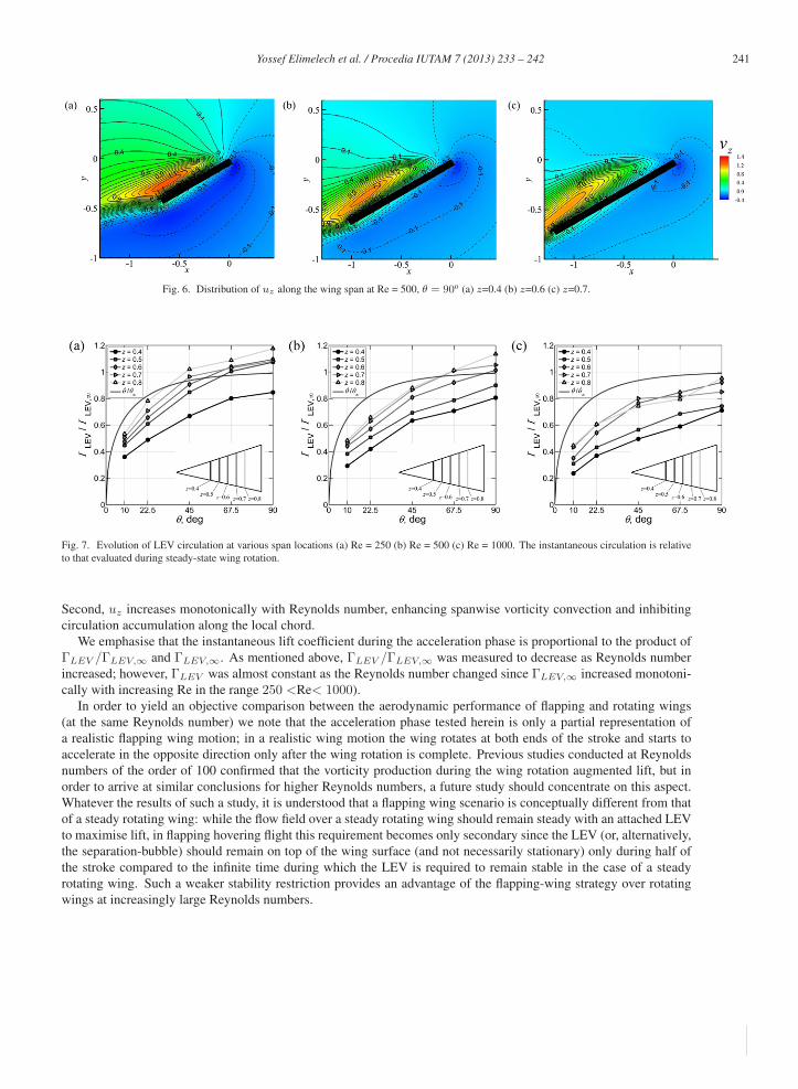
was also non-uniformly distributed along the wing span, as shown in Fig. 6 for Re = 500 at θ = 90o. The highest uz

was measured near the wing root (Fig. 6a), and it decayed monotonically along the span towards the wing tip (Fig. 6c).

Interestingly, uz was not confined to the region where ωz was maximal (i.e. within the LEV region); this phenomenon

is at variance with earlier discussions which have associated the stability of an LEV solely with the presence of high

spanwise flow within the LEV core; in a case where the LEV stability was solely uz dependent, higher values of uz

should have been associated with an attached LEV. In turn, the current results at Re = 2000 showed a non-stationary

dual-core LEV (Fig. 2d) while uz peaked to its highest value at that Reynolds number. Therefore, we suggest that the

fluid viscosity (which of course affects the local Reynolds number at each span location) is another key factor which

may inhibit the growth-rate of possible flow disturbances and preserve the LEV coherence.

In order to describe the role of the spanwise flow, we show its correlation with the vorticity production within the

LEV. To this end, ωz within the LEV was integrated during the acceleration phase and thereafter during the steady

rotation, yielding the LEV circulation; its evolution is described below as the ratio between the instantaneous circula-

tion and that obtained during steady wing rotation, ΓLEV /ΓLEV,∞. ΓLEV,∞ was calculated from flow measurements

acquired following five successive periods of steady wing rotation. The evolution of the LEV circulation is presented

in Fig. 7 for three different Reynolds numbers. The initially high circulation growth rate is explained by the fact

that the spanwise velocity component was small at the initial stage of the wing motion (Fig. 5a). The low spanwise

velocity induced low vorticity convection towards the tip and encouraged vorticity accumulation. Only later, when the

spanwise velocity component grew considerably, did the growth rate of ΓLEV decay following the same mechanism.

The evolution of uz also explains the differences in the LEV circulation growth along the span: at the middle of the

stroke ΓLEV approached approximately its steady-state value at the most distal span station, z = 0.8, (Fig. 7) while

at the most medial span station (z = 0.4) ΓLEV reached only 80 percent of its ultimate steady-state value at the same

instant.

Interestingly, at the lowest end of the Reynolds number range (Re = 250), the circulation evolution during the accel-

eration phase showed some aerodynamic benefits since the circulation attained a level which exceeded its asymptotic

steady wing rotation value. The results clearly show that ΓLEV /ΓLEV,∞ decreases as Reynolds number increases

(Fig. 7); we believe that two effects contribute to this phenomenon: first, the separation-bubble region is consider-

ably longer at larger Reynolds numbers; a longer time is therefore needed to convect vorticity in the chord direction.

1The flow field is also fully three-dimensional near the wing tips; however, this feature is generally present in the flow over a translating finite

wing as well as in that over a rotating finite wing.


Fig. 3. Flow field evolution at Re = 250 (left panels) and Re = 1000 (right panels), z=0.6, during the wing acceleration, showing contours of

ωz . (a,d) θ = 10o; (b,e) θ = 45o; (c,f) θ = 90o. For clarity, only representative velocity vectors are shown. Gray shading indicates the

light-sheet-shadow regions.


Fig. 4. Representative comparison between the experimental (top row) and numerical (bottom row) results, Re = 500 at z = 0.5 at two stations

during the acceleration phase. The compared quantity is ωz . In-plane vector field is superposed on the experimental results; the numerical results

depict contour levels of uz in addition to ωz contours. (a,c) θ = 10o; (b,d) θ = 90o.

Fig. 5. Evolution of uz at Re = 500, z=0.4 during wing acceleration, showing contours and contour levels of the dimensionless spanwise velocity

(a) θ = 10o, (b) θ = 45o, (c) θ = 90o.


Fig. 6. Distribution of uz along the wing span at Re = 500, θ = 90o (a) z=0.4 (b) z=0.6 (c) z=0.7.

Fig. 7. Evolution of LEV circulation at various span locations (a) Re = 250 (b) Re = 500 (c) Re = 1000. The instantaneous circulation is relative

to that evaluated during steady-state wing rotation.

Second, uz increases monotonically with Reynolds number, enhancing spanwise vorticity convection and inhibiting

circulation accumulation along the local chord.

We emphasise that the instantaneous lift coefficient during the acceleration phase is proportional to the product of

ΓLEV /ΓLEV,∞ and ΓLEV,∞. As mentioned above, ΓLEV /ΓLEV,∞ was measured to decrease as Reynolds number

increased; however, ΓLEV was almost constant as the Reynolds number changed since ΓLEV,∞ increased monotoni-

cally with increasing Re in the range 250 <Re< 1000).

In order to yield an objective comparison between the aerodynamic performance of flapping and rotating wings

(at the same Reynolds number) we note that the acceleration phase tested herein is only a partial representation of

a realistic flapping wing motion; in a realistic wing motion the wing rotates at both ends of the stroke and starts to

accelerate in the opposite direction only after the wing rotation is complete. Previous studies conducted at Reynolds

numbers of the order of 100 confirmed that the vorticity production during the wing rotation augmented lift, but in

order to arrive at similar conclusions for higher Reynolds numbers, a future study should concentrate on this aspect.

Whatever the results of such a study, it is understood that a flapping wing scenario is conceptually different from that

of a steady rotating wing: while the flow field over a steady rotating wing should remain steady with an attached LEV

to maximise lift, in flapping hovering flight this requirement becomes only secondary since the LEV (or, alternatively,

the separation-bubble) should remain on top of the wing surface (and not necessarily stationary) only during half of

the stroke compared to the infinite time during which the LEV is required to remain stable in the case of a steady

rotating wing. Such a weaker stability restriction provides an advantage of the flapping-wing strategy over rotating

wings at increasingly large Reynolds numbers.


4. Conclusions

A combined experimental-numerical study has been undertaken to analyse the vorticity production over an accel-

erating wing at various Reynolds numbers. The good comparison between the experimental and numerical results

allowed use of the spanwise velocity component which was resolved numerically in order to describe the essential

flow mechanisms involved. At Reynolds numbers higher than 250 the vorticity was not confined to the vicinity of the

leading-edge and remained stable up to a Reynolds number between 1000 and 2000. The evolution of the spanwise

velocity component was found to be correlated with the growth of circulation; higher spanwise velocity at larger

Reynolds numbers was characterised by slower time evolution of the LEV circulation over the wing.

The results presented here show that at Re = 250 the LEV circulation exceeds its steady-state value when the wing

approaches the middle of the stroke (θ = 90o). At Re = 1000, by contrast, the LEV circulation during the acceleration

phase was found to stay considerably below its asymptotic steady wing rotation value. This finding demonstrates that

at Reynolds numbers of a few thousand the aerodynamic performance of a flapping wing cannot be well described by

a steady rotation analysis which overestimates the actual aerodynamic wing performance.

Most importantly, the results highlight the aerodynamic advantage of flapping flight (over steady wing rotation) at

Reynolds numbers above 1000; whereas the LEV becomes unstable during steady wing rotation, the flapping strategy

limits the time during which the LEV has to remain stable (or marginally stable) because the LEV is shed by the

wing rotation at each end of the half stroke and is then renewed. Each half stroke is thus characterised by a high lift

(associated with the LEV) that cannot be attained with steady wing rotation. It is believed that the wing rotation at

each end of the half stroke (at Re > 250) can produce additional lift and be advantageous to the flapping wing strategy.

Acknowledgements

Y.E. was supported in part by the Joan and Reginald Coleman-Cohen Fund. Numerical simulations were carried

out using HPC resources of IDRIS, Paris, project 81664.

References

[1] Weis-Fogh T. Quick estimates of flight fitness in hovering animals including novel mechanisms for lift production. The Journal of ExperimentalBiology. 1973;59:169–230.

[2] Van-Den-Berg C, Ellington CP. The three-dimensional leading-edge vortex of ‘hovering’ model hawkmoth. Phil Trans R Soc Lond B.

1997;352:329–340.

[3] Ellington CP, Van-Den-Berg C, Willmott AP, Thomas ALR. Leading-edge vortices in insect flight. Nature. 1996;384:626–630.

[4] Bomphrey RJ, Lawson NJ, Harding NJ, Taylor GK, Thomas ALR. The aerodynamics of Manduca sexta: digital particle image velocimetry

analysis of the leading-edge vortex. The Journal of Experimental Biology. 2005;208:1079–1094.

[5] Maxworthy T. The formation and maintenance of a leading-edge vortex during the forward motion of an animal wing. Journal of FluidMechanics. 2007;587:471–475.

[6] Lentink D, Dickinson MH. Rotational accelerations stabilize leading-edge vortices on revolving fly wings. The Journal of ExperimentalBiology. 2009;212:2705–2719.

[7] Usherwood JR, Ellington CP. The aerodynamics of revolving wings. II. Propeller force coefficients from mayfly to quail. The Journal ofExperimental Biology. 2002;205:1547–1564.

[8] Poelma C, Dickson WB, Dickinson MH. Time-resolved reconstruction of the full velocity field around a dynamically-scaled flapping wing.

Experiments in Fluids. 2006;41:213–225.

[9] Dalziel SB. DigiFlow User Guide. Dalziel Research Partners; 2003–2009.

[10] Kolomenskiy D, Moffatt HK, Farge M, Schneider K. Two- and three-dimensional numerical simulations of the clap-fling-sweep of hovering

insects. Journal of Fluids and Structures. 2011;27(5–6):784–791.

[11] Angot P, Bruneau CH, Fabrie P. A penalisation method to take into account obstacles in viscous flows. Numerische Mathematik. 1999;81:497–

520.

[12] Schneider K. Numerical simulation of the transient behaviour in chemical reactors using a penalisation method. Method Comput Fluids.

2005;34:1223–1238.

[13] Davidson PA. Turbulence: An introduction for scientists and engineers. Oxford University Press; 2004.

[14] Himmelskamp H. Profile investigation on rotating airscrew. Dissertation Gottingen; 1947.