1
Evaluation of Segmentation Techniques for Inventory Management in Large Scale Multi-Item Inventory Systems1
Manuel D. Rossetti2, Ph. D., P. E. Department of Industrial Engineering
University of Arkansas 4207 Bell Engineering Center
Fayetteville, AR 72701
Ashish V. Achlerkar, M.S. MCA Solutions, Inc.
2 Penn Center Plaza (1500 JFK Blvd.) Suite 700
Philadelphia, PA 19102
Abstract This paper presents and evaluates methodologies for the segmentation or grouping of items and the subsequent setting of their inventory policies in a large-scale multi-item inventory system. Conventional inventory segmentation techniques such as ABC analysis are often limited to using demand and cost when segmenting the inventory into groups for easier management. Other attributes may be of functional and operational importance when deciding inventory control policies. Considering other attributes while forming item-groups may ensure group policies that achieve the desired performance metrics for a given inventory system while respecting cost considerations. Two segmentation methodologies, (Multi-Item Group Policies (MIGP) and Grouped Multi-Item Individual Policies (GMIIP), that use statistical clustering algorithms were developed and compared to the conventional ABC analysis technique. An empirical evaluation of these techniques via a set of experiments was performed. The analysis indicates that these new techniques can improve inventory management for large-scales systems when compared to ABC analysis. Keywords: multi echelon inventory, inventory segmentation, clustering.
1 Accepted for publication in the International Journal of Logistics Systems Management 2 Corresponding author. Tel.: 479-575-6756; fax: 479-575-8431. Email address: [email protected]

2
Biographical Notes
Manuel D. Rossetti, Ph.D., P.E., has published over 70 refereed articles in the areas of transportation, logistics, manufacturing, health care, and simulation and obtained over $3.4 million in funding from, among others, the National Science Foundation, Air Force Research Lab, the U. S. Navy, and Wal-Mart Stores, Inc. He was selected as a Lilly Teaching Fellow in 1997/98 and won the IE Department Outstanding Teacher Award in 2001-02 and 2007-08. He has served as co-editor for the 2004 and 2009 Winter Simulation Conference and is the author of the textbook, Simulation Modeling and Arena published by John Wiley & Sons. Ashish V. Achlerkar is a senior consultant for MCA Solutions Inc. He has over 6 years of experience providing supply chain solutions to customers from Aerospace/Defense and commercial industries. He has served in MCA’s Product Management service during which he successfully led several product development efforts. He has also performed research in the area of multi-echelon, multi-indenture inventory optimization. Prior to joining MCA, he worked for Bajaj Auto Ltd, an Asian automobile giant. He holds a Bachelors in Engineering degree from the College of Engineering Pune (COEP), India and a Masters of Science degree from the University of Arkansas, Fayetteville.
Acknowledgements Thanks to the anonymous reviewers for their suggestions to improve the article. This material is based upon work supported by the National Science Foundation under Grant No. 0437408. Any opinions, findings, and conclusions or recommendations expressed in this material are those of the author(s) and do not necessarily reflect the views of the National Science Foundation.
3
Evaluation of Segmentation Techniques for Inventory Management in Large Scale Multi-Item Inventory Systems
Abstract This paper presents and evaluates methodologies for the segmentation or grouping of items and the subsequent setting of their inventory policies in a large-scale multi-item inventory system. Conventional inventory segmentation techniques such as ABC analysis are often limited to using demand and cost when segmenting the inventory into groups for easier management. Other attributes may be of functional and operational importance when deciding inventory control policies. Considering other attributes while forming item-groups may ensure group policies that achieve the desired performance metrics for a given inventory system while respecting cost considerations. Two segmentation methodologies, (Multi-Item Group Policies (MIGP) and Grouped Multi-Item Individual Policies (GMIIP), that use statistical clustering algorithms were developed and compared to the conventional ABC analysis technique. An empirical evaluation of these techniques via a set of experiments was performed. The analysis indicates that these new techniques can improve inventory management for large-scales systems when compared to ABC analysis. 1 Introduction Williams and Tokar (2008) provide a review of inventory management issues that have
appeared in the literature. They classify the literature into the inventory models,
collaboration control, stock out assumptions, and demand assumptions. An important
issue that has been missing in the literature is the modeling of large-scale inventory
systems. Large-scale inventory systems have as their primary characteristic a significant
number of SKUs. A SKU is an individually managed item type, for which a quantity of
inventory is stored and managed at a particular location. Only 17 years ago, Moore and
Cox (1992) considered issues in forecasting for large-scale inventory systems, with
examples that ranged between only 250 and 80,000 SKUs. Today, many inventory
systems easily have hundreds of thousands of SKUs. For example, Lowe’s Companies,
Inc. was recently given a Voluntary Interindustry Commerce Solutions (VICS)

4
achievement award for being able to “forecast demand for more than 42 million
store/SKUs, creating a time-phased, flexible approach to adjusting to changing consumer
demand, and sharing the data with suppliers” (Margulis (2009)).
In very large inventory systems, it may not be feasible to set stock levels and
service control guidelines for each individual item. Inventory management resources may
be better utilized by managing the “significant few” and not the “trivial many”. Such an
approach to inventory management may be achieved by the classification and grouping of
inventory items and subsequent assignment of inventory policies according to the
characteristics of a group. Classification systems serve to prioritize inventory items by
certain criteria and allow expenditure of management resources in proportion to an item’s
value in the system.
The characteristics of the groups of items formed depend upon the type and
number of attributes considered while forming the groups. Conventional grouping
techniques like ABC analysis give importance to the cost and demand volume attributes
of items during grouping. Techniques such as group technology give importance to the
physical attributes of items during grouping so as to achieve convenience during
manufacturing operations, not necessarily for inventory policy determination. There are
several other attributes of items in inventory systems that are critical in deciding
inventory policies. These attributes are of operational significance when it comes to
meeting strategic and operational objectives. In order to obtain balanced, practical, and
operationally useful groups of items in an inventory system, it is important to consider
item-attributes that contribute to inventory management goals.
5
Clustering is a technique that is used to classify objects into groups based on their
attributes. Different clustering techniques are defined depending on the mathematical
algorithms used to classify objects into groups. The basic objective of clustering
algorithms is to form groups of objects that exhibit minimum within-group variability and
maximum between-group variability. The concept of clustering can be applied to the
inventory segmentation problem to form groups of items that have similar inventory
policy parameters. Selecting appropriate item attributes to be used in the clustering
algorithm is important to obtain groups of items that show high homogeneity between
items in a given group. Once such groups of items are formed, common inventory
policies for all the items in a group may be applied. This may enhance managerial
convenience for overall system control since it is necessary to determine policies and
manage only a small number of “groups of items” instead of managing every item
individually.
On the other hand, because group policies are used instead of individual policies
while managing inventory items, there is a loss of identity for the items. This loss of
identity suggests a penalty cost that has to be incurred as a result of using group policies
instead of individual policies. Also, there might be an undesired change in the values of
several performance metrics if the penalty cost is minimized. It is important that the
groups resulting from the application of segmentation or clustering techniques still meet
the cost and performance goals. The managerial convenience obtained by grouping items
has to be traded-off with the penalty cost and performance metric values associated with
the system. This is a challenge for inventory managers and strategic planners.

6
From this paper, the reader should develop a better understanding of the issues
and trade-offs involved in inventory segmentation for large-scale inventory systems. In
addition to explaining and illustrating many of the issues, this paper develops and
compares methodologies for segmenting inventory for multi-item single echelon large-
scale inventory systems. Two new segmentation methodologies (Multi-item Group
Policies, MIGP and Grouped Multi-item Individual Policies, GMIIP) that use statistical
clustering algorithms are compared to the conventional ABC analysis technique. The
examination of a multi-item single echelon large-scale inventory system allows an
analysis without the complications of having to set policies in a multi-echelon setting and
provides a foundation for addressing large-scale multi-item, multi-echelon systems.
The paper is organized as follows. In the next section, background on the
inventory segmentation problem is presented by reviewing relevant literature. Section 3
describes the methods (MIGP and GMIIP) for segmenting and assigning the inventory
policies. Section 4, presents the experimental procedures and discusses the results.
Finally, Section 5 summarizes the findings and discusses the possibilities for future
research.
2 Background and Literature Review In large supply networks (e.g. Wal-Mart, US-Navy, etc.) hundreds of thousands of items
are stocked at a single location or echelon within a larger supply chain. These types of
inventory systems (e.g. multi-echelon, multi-item) with millions of items throughout the
network are considered large-scale inventory systems. Calculating the optimal inventory
policy parameters for large-scale inventory systems is a computational burden that
necessitates the need for efficient policy setting techniques that reduce the computational
7
time, and at the same time improve the ability of inventory managers to more effectively
manage the supply chain. Because of these challenges extensive research has been
performed on how to optimally set inventory policy parameters within these contexts.
The purpose here is not to review that body of work. The reader interested in that topic
can refer to Deuermeyer and Schwarz, (1981), Svoronos and Zipkin (1988), Zipkin
(2002), Cohen et al. (1990), Hopp et al. (1999), Caglar et al., (2004), Al-Rifai and
Rossetti (2006), and Muckstadt (2005) and the references therein, for a basic introduction
and overview of this area. See also Gümüs and Güneri (2007) for a recent review with 92
references.
In this background section, the discussion is focused on two papers that are
directly relevant to this paper: Hopp et al. (1997) and Cohen and Ernst (1986). Hopp et
al. (1997) and subsequently Hopp and Spearman (2001) serve as the basis for the policy
setting methodology used in this paper in order to test the effectiveness of the inventory
segmentation techniques.
Research on grouping methods within inventory systems dates at least back to
1981 where Chakravarty (1981) examined classifying SKUs into a few manageable
groups that have a common order cycle or common order quantity. The approach
involves finding a common policy parameter given a pre-specified number of items in
each group. The grouping problem was formulated as a non-linear program and solved
via dynamic programming. The results confirm the common notions of ABC
classification found in industry. Leonard and Roy (1995) call for the gap between
inventory theory and practice to be reduced by having “items grouped into coherent
families using a structure of attributes which are both theoretical and practical” and then
8
building “an aggregate item representative of the different items of the family in order for
the practitioner to take his decisions”. Partovi and Anandarajan (2002) used neural
networks to classify stock keeping units within the pharmaceutical industry into A, B,
and C type items. Other work in this area has focused primarily on multi-attribute
classification (Ramakrishnan (2006), Zhou and Fan (2007), Chu et al. (2008)) to find
management groups, but not integrated with policy setting.
Cohen and Ernst (1986) is the first paper (to our knowledge) that begins to
address the inventory segmentation problem and its implications. Cohen and Ernst
(1986) developed a methodology to group spare parts based on statistical clustering
constrained by operational performance criteria, which they termed (ORG) for
operational relevant groups. Their clustering technique considers many attributes used in
functional grouping going beyond the conventional cost and volume attributes used in
ABC analysis. The paper uses a classical statistical grouping problem that attempts to
assign items to groups with the following properties: minimum within group variance for
each variable, maximum between group variance for each variable, and a limited or
constrained number of groups. The paper uses statistical techniques to try to maximize
the degree of dissimilarity (D) amongst the groups based on the proportion of variance
accounted for by the clusters. The statistical clustering problem, as described in the paper,
then requires finding the set of clusters that maximize D subject to a constraint on the
maximum number of groups.
Cohen and Ernst (1986) suggest three steps to solve this optimization problem:
sample selection and preliminary data analysis, data reduction by factor analysis, and
group generation by cluster analysis. The paper gives a method to balance the cost
9
penalties and the loss of individual item identity due to grouping against the reduction in
computational and managerial efforts due to grouping. The operations based analysis
described in the paper has two objectives: (1) find the groups that minimize the cost/and
operational performance penalty for group based generic control policies, and 2) restrict
the maximum number of groups to be less than or equal to a managerial and
computational maximum. The grouping problem was then reformulated to be
operationally constrained. The revised grouping problem attempts to minimize the total
number of groups subject to a constraint on the maximum operational penalty.
The revised problem of Cohen and Ernst (1986) has a non-linear constraint and
was solved using a special hierarchical approach. The membership function was
determined using discriminant analysis and Euclidean distance coefficients were used as
a measure of dissimilarity amongst groups. The paper gives consideration to the impact
of the grouping scheme on the policies to be developed with the aid of the groups. The
experiments conducted for the inventory system of a vehicle manufacturer using the ORG
technique showed superior results when compared to conventional grouping techniques.
The need to define groups in a manner that reflects trade-offs among statistical
performance, operational performance, data needs, and computational requirements is the
key connection to the work presented here. This research also uses statistical clustering,
but trying to fully solve the clustering problem and the policy-setting problem at the same
time is not attempted. The methodology presented in this paper is meant to be heuristic
and primarily illustrative, but certainly points to how segmenting and policy setting can
be integrated. The idea is straightforward: segment the items, set inventory policies, and

10
examine the cost penalties associated with resulting groups. In order to set the inventory
policies, the methodology presented in Hopp and Spearman (2001) was used.
Hopp and Spearman (2001) presents an algorithm for a multi-item (R, Q) backorder
model that computes the inventory policy parameters at a single location that is faced
with Poisson demands and assumed fixed lead times. The notation for this model is as
follows:
i = Item index
N = Number of items
€
F = Target order frequency (orders per year)
€
B = Target number of backorders
€
λi = Item i demand rate (units/year)
€
Li = Item i lead time (ordering and transportation)
C = Total inventory investment ($)
€
hi = Item i holding cost ($/item) = holding cost rate times unit cost
€
Qi = Item i replenishment batch size (units)
€
Ri = Item i reorder point (units)
€
I i Ri ,Qi( ) = Item i average on-hand inventory (units)
€
B i Ri ,Qi( ) = Item i expected number of backorders (units)
P1:
€
Minimize C = hi I ii=1
N
∑ Ri ,Qi( ) (1)
Subject to
€
1N
λi
Qii=1
N
∑ ≤ F (2)

11
€
B i Ri ,Qi( )i=1
N
∑ ≤ B (3)
€
Ri ≥ −Qi ,i = 1, 2 …N (4)
€
Qi ≥1,i=1,2,...N (5)
(6)
The resulting mathematical program attempts to minimize the total inventory
holding cost subject to expected annual order frequency and expected number of
backorder constraints. In this model, it is unnecessary to specify a backorder cost because
the model formulates the customer service requirement as a constraint involving the total
backorder level. This is also a surrogate for customer wait time because of Little’s
formula. Hopp and Spearman (2001) suggest an iterative procedure to solve this
optimization problem. In this procedure, they first satisfy the average order frequency
constraint and then satisfy the backorder level constraint. Since the order frequency
depends upon the order quantity
€
Qi alone, once the procedure finds a
€
Qi that gives an
average order frequency as per the required value, the procedure proceeds to satisfy the
second constraint on the backorder level. The total backorder level depends upon both the
order quantity and the reorder point. So with the optimal order quantity obtained while
satisfying the first constraint, a reorder point that satisfies the backorder constraint can be
found. The algorithm suggested by Hopp and Spearman (2001) and can be implemented
using a binary search procedure on the Lagrange multipliers in the constrained
optimization problem that represent the imputed setup and backorder costs.
For a large-scale inventory system, deciding optimal inventory policies expends
much computational time and resources. The idea behind inventory segmentation
procedures is to group items into families based on some important attributes, and then

12
apply common generic control policies to those part-families. This may greatly reduce
the computational and operational efforts required in managing the items. In an
inventory segmentation process, the idea is to group items that are “most” similar
together. So the attribute values for items in the same group will be similar but not
exactly alike. This within-group similarity between items in the same group depends on
the level of similarity at which the groups are formed using clustering algorithms. So
there is bound to be at least some minor dissimilarity between items in the same group.
If common inventory policies are applied to items in the same group, then a cost
penalty will result because optimal policies are not set individually. It is important to note
that there is a loss of identity for items due to using group policies. The loss of identity by
items can be measured by a penalty cost and/or undesired change in the values of
performance metrics when group policies are used instead of individual policies. As the
number of groups increases, the more will be the similarity between items in the same
group and hence less will be the loss of identity for items. But at the same time managing
a larger number of groups means less managerial convenience while managing inventory
and hence less benefit from inventory segmentation. This trade-off between the effect of
the loss of identity of the items and the benefits of segmentation is of key interest in this
paper.
Most of the conventional inventory classification techniques such as ABC
analysis consider only limited number of attributes while forming classes of items. This
research examines inventory segmentation techniques that consider operationally relevant
attributes while classifying inventory items. Also, this research focuses on establishing an
effective trade-off between managerial convenience via clustering with the penalty cost
13
and overall supply chain goals as a result of using group policies. The next section
presents methodologies that allow the examination of these trade-offs.
3 Inventory Segmentation Methods In this paper the inventory segmentation methods are applied to the control of single
echelon, multi-item, large-scale inventory systems. The basic approach is: 1) cluster the
items into groups, 2) apply inventory policy setting algorithms, and 3) measure the
cost/performance trade-offs. This section describes the specifics of these steps. Since the
approaches depend upon clustering it is important to start with the underlying
characteristics of the inventory systems.
3.1 Characteristics of the Inventory Systems
Based on the characteristics of items in an inventory system, inventory systems can be
categorized into different types. For example, an inventory system might consist
primarily of repairable items, consumable items, perishable items, or some combination
of these types of items. Each of these types of inventory system will have definite
characteristics when the item attribute values and the relationships between the attributes
are considered. Thus, to perform the segmentation of the items, the different attributes of
the items need to be considered.
This research considers inventory systems that can be roughly classified as
repairable, consumable or both. Table 1 summarizes the assumptions regarding the
characteristics of the different types of inventory systems while Table 2 quantifies the
attributes that are considered. In Table 1, repairable item inventory systems have items
that are characterized by high unit costs, low average annual demand, high replenishment
lead times, low mean lead time demand, high variance of lead time demand, high desired
14
fill rate, high essentiality values, and high criticality values. The quantification of
attribute categories is based on a study of datasets used by Deshpande et al. (2003) in
their study on the inventory system of the Defense Logistics Agency (DLA). In Table 2,
the attribute value categories are given. For example, from Table 2, it can be noted that if
the attribute category value of unit cost for items in a given inventory system is defined
as high, the items in such an inventory system should have unit cost values ranging from
$50,000 to $100,000. The other attributes and their categories can be interpreted in a
similar fashion. These attributes and categories for the different types of inventory
systems will be used during the clustering analysis and as part of a data generation
procedure used in the experiments to make inferences concerning how well the
segmentation methods perform for different types of systems and item types.
Table 1 and Table 2 placed near here
Assuming an inventory system that has many items that have the characteristics given in
Table 1 and 2, the next step is to consider methods for grouping or clustering the items
and setting policies
3.2 Issues related to Grouping or Clustering the Items
The most frequently used inventory classification scheme is ABC inventory
classification. This classification is based on ranking the items by the product of each
item’s annual demand and its unit cost. Typically, approximately 20% of items account
for about 80% of the total annual dollar usage (Silver et al. (1998)). Classification of
items is also often performed within the application of group technology, primarily based
on physical or other characteristics that are important in the production process. The type
of groups obtained using such techniques may satisfy limited goals of the overall supply
15
chain; however, in practice there may be many other objectives that need to be satisfied.
Thus, it is important to try to group items based on additional operationally and
functionally important attributes so as to obtain practical groups. Clustering algorithms,
which have not been traditionally applied to the area of inventory management, can be
used for this purpose.
The main clustering method used in this research is the Unweighted Pair Group
Method Using Arithmetic Averages or the UPGMA clustering method. During the
experimentation, the performance of the K-means clustering algorithm is also examined.
Statistical Analysis Software (SAS) was used for the clustering of the datasets.
Romesberg (1984) gives the steps in clustering problems: 1) attribute selection, 2) data
matrix formation and standardization, 3) computing similarity metrics, and 4) forming the
clusters. In addition, Romesberg (1984) describes the UPGMA and K-means algorithms.
UPGMA is a hierarchical form of clustering. In a hierarchical clustering technique the
data are not partitioned into a particular number of classes or clusters at a single step.
Instead the classification consists of a series of partitions, which may run from a single
cluster containing all individuals, to n clusters each containing a single individual. The
key issues for this research are 1) attribute selection, 2) the number of clusters, and 3)
similarity metrics. The attributes examined are given in Table 1. The usefulness of
various attributes to the formation of clusters and number of clusters are examined within
the experiments. The similarity metric used here is the Euclidean distance coefficient
based on the standardized attribute values. See Everitt et al. (2001). Given a method for
forming groups is available, the next important issue is how to incorporate the groups
16
into a policy setting procedure. The next two sections discuss alternative methods for
when and how to use the groups in the inventory segmentation problem.
3.3 Multi-Item Group Policies (MIGP) Inventory Segmentation
The inventory segmentation problem is how to form groups and how to set policies. The
MIGP methodology: 1) groups inventory items based on some attributes using a
clustering algorithm, 2) determines an inventory policy for each group (i.e. determines a
group policy), and 3) has each item within each group use the group policy for its
individual inventory policy. In this approach, step 2 is accomplished by applying the
multi-item back order model (P1) to the groups. This effectively reduces the size of the
optimization problem where N is now the number of groups rather than the number of
items. A key issue in this procedure is how to determine the other parameters of the
optimization problem (e.g. item demand rate, lead time, holding cost, etc.) for each group
prior to applying the optimization procedure. This is denoted as the group policy
deciding criteria. For example, let
€
G j represent the set of items in group
€
j having
€
m j = G j as the number of items in the group. Then, if the group policy deciding criteria
is the average of the attribute values of items in the group then
€
L jg = 1 m j( ) Lii∈G j
∑ represents the lead time of group
€
j in the multi-item back order
optimization problem.
Clearly, there is a trade-off associated with the computational savings associated
with solving the optimization problem based on groups and the use of the group’s
inventory policy on the individual items within the group. If the items are truly similar,
then applying a group policy may not cause a significant increase in total cost or decrease
in performance when compared to solving each item’s optimal policy parameters. In

17
addition, it is easier to manage a smaller number of groups than potentially hundreds of
thousands of individual items.
3.4 Grouped Multi-Item Individual Policies (GMIIP) Inventory Segmentation
In the MIGP inventory segmentation methodology, after the items are grouped a group
policy deciding criteria is applied and then the optimization problem is solved on the
groups. The GMIIP segmentation methodology implements the same logical steps as the
MIGP segmentation methodology with one major change. Instead of using a group policy
deciding criteria, the GMIIP methodology calculates individual inventory policies for
every item within the groups. The statistical clustering algorithm serves the purpose of
providing inventory groups that are versatile, practical, and operationally useful. Once
the right number and type of groups are formed, these groups are treated as separate sub-
problems for the multi-product backorder model.
The complex problem involving policy calculations for a large number of items has
now been broken down into several smaller problems. This permits each sub problem to
be more readily (quickly) solved. While this achieves managerial convenience with some
extra computational cost to solve each sub problem, the items do not lose their total
identity because they have their own individual policies. The only loss of identity that
the items experience is due to the interactions in the multi-item backorder model. This is
because the sub-problems are solved individually and the items within different groups
no longer compete within the constraints. Thus, the GMIIP segmentation methodology
makes it possible to eliminate one major factor for the loss of identity of the items. At the
same time (hopefully) achieving more practical and operationally useful inventory groups
than those formed by the conventional inventory grouping techniques like ABC analysis.
18
The GMIIP technique may yield an inventory segmentation solution that gives a lower
penalty cost than the MIGP technique but with increased computation.
In the next section, a set of experiments is used to understand the effectiveness of the
MIGP and GMIIP methods by computing the penalty cost and computation times
associated with any loss of optimality for not solving the entire multi-item back order
problem.
4 Experiments and Results
This section discusses the experiments and the results of the analysis. The overall goal is
to gain insights by comparing the performance of the MIGP, GMIIP and ABC analysis
techniques with respect to performance metrics like penalty cost, execution time for
policy calculations, fill rate and customer wait time. The clustering process can be
sensitive to the characteristics of the inventory system, thus it is also important to
examine the factors involved in the inventory segmentation process for different types of
inventory systems when considering the effectiveness of the segmentation procedures. In
order to be able to test the performance of the methods, a procedure is needed that can
generate problem instances for the segmentation processes.
4.1 Data Generation Procedure
A procedure to generate problem instances for testing purposes was developed based on
the discussion in Section 3 (Tables 1 and 2). In order to develop a method to generate
artificial datasets that contain relationships between the generated values of various
attributes some assumptions between the attributes based on experience and Deshpande
et al. (2003) were made:
• The average annual demand is inversely proportional to the unit cost of an item.
• The average annual demand is inversely proportional to the replenishment lead-time.

19
• The average annual demand directly proportional to the mean demand during the
replenishment lead-time.
• The average annual demand is directly proportional to the variance of demand during
the replenishment lead-time.
• The average annual demand is directly proportional to the essentiality of the item.
• The average annual demand is directly proportional to the criticality of the item.
• The average annual demand is directly proportional to the desired fill rate of the item.
These assumptions are based on reasonable intuitive notions that are expected in typical
inventory system datasets. For example, high demand items will tend to have low unit
costs. In addition, high demand items tend to have lower lead times. For high demand
items, it is intuitive that the mean demand during the lead-time and the variance of
demand during the lead-time will tend to be high and hence these two attributes were
considered to be directly proportional to the attribute “demand”. Highly essential items
will be procured more and hence they tend to have a high annual demand. Similarly
highly critical items will also tend to be procured more and hence will have high demand.
This helps to explain the assumption regarding the relationship between the pairs of
attributes “demand and essentiality” and “demand and criticality”. Those items for which
the value of the attribute desired fill-rate is very high will tend to be procured more and
hence may tend to exhibit a higher annual demand. This helps to explain the assumption
regarding the relationship between the attributes “average annual demand” and “fill-rate”.
Based on the above assumptions a procedure was developed to randomly generate
datasets with desirable characteristics based on a sequence of conditional probability
distributions. Table 3 contains an example specification for generating attribute values

20
for an inventory system. For example, in Table 3, the attribute average annual demand is
stratified into 3 strata ([1, 1000] low demand, [1000-5000] medium demand, [5000-
10000] high demand). A probability distribution is specified across the strata (in this
example it is equally likely (33%) to get demand from a particular stratum). Once the
stratum is chosen, then the attribute value is randomly generated from the stratum using a
uniform distribution over the stratum’s range. This process continues for each of the
other attributes.
Table 3 placed near here
For example, suppose the high average annual demand stratum was randomly selected, to
generate the lead-time, one of the strata for the lead-time values must then be chosen.
Once that stratum is chosen, a value for the lead-time is then drawn. The strata and
allocation of probability across the strata were set based on the previously described
intuitive assumptions. For example, the low stratum for lead-time has an 80% chance of
being selected for high demand items. Thus, the procedure will tend to generate high
demand items with low lead-time values. Other strata for the attributes criticality, size,
weight, and fill-rate were also used, but not shown here due to limitations on space.
It should be clear that this procedure will not represent any particular real
inventory system (and readers may question the ultimate validity of the assumptions);
however, that is not the point. The point is to be able to generate reasonable large-scale
datasets (with some control over their properties) such that a relative comparison
between the segmentation methods can be examined. In the experiments, different
allocations for the conditional probability distributions for the strata as well as ranges for
the strata were examined to attempt to mimic different kinds of inventory systems. Such

21
a data generation procedure is necessary in order to allow experimentation involving such
factors as the type of inventory system, number of items, etc. as well as to gain some
understanding into the importance of various attributes during the clustering procedure.
While it may be preferable to test on real data sets, real data sets do not permit easy
control over a wide range of attribute values. To our knowledge, no such data generation
procedure is described elsewhere in the literature. The procedure used in this research
represents a first step at developing an important component for testing algorithms and
methods for large-scale inventory systems. Once datasets can be generated, experimental
analysis of the effect of the segmentation strategies can be completed.
4.2 Screening and Segmentation Experiments
In order to examine the effectiveness of the MIGP and GMIIP procedures a two-phase
experimental plan was developed. The first phase involves a set of screening
experiments to understand the basic behavior of the responses and to establish important
factors for further investigation. The second phase of the analysis examined a prioritized
response function to try to develop recommendations as to the most appropriate
segmentation strategy given different types of datasets.
The key responses to be considered during both phases are:
• Penalty cost – The total inventory cost increase due to setting the policies based
on a segmentation strategy.
• Execution time – The time to execute the policy setting algorithm.
• Average fill rate – The average fill rate achieved for the items.
• Customer wait time – The average customer wait time achieved for the items.
22
Penalty cost, average fill rate, and customer wait time provide insights into the trade-offs
for cost and service due to the application of the segmentation techniques. Execution
time provides a surrogate for ease in managing the items.
4.2.1 Screening Experiments and Results Because the purpose of the experiments is to screen factors, only the MIGP procedure
was analyzed. In this analysis, the following factors are of interest:
• Algorithm based factors: number of clusters, clustering algorithm, group policy
deciding criteria. For number of clusters, the levels are high [80% of the total
number of SKU’s in the data set], and low [20% of the total number of SKU’s in
the data set]. For the clustering algorithm the UPGMA method was compared to
the K-means method. For the group policy deciding criteria, using the mean of
the group is compared to using the median of the group for policy setting was
compared.
• Attribute based factors: unit cost, average annual demand, replenishment lead-
time, mean lead-time demand, variance of lead time, essentiality, criticality, item
size, item weight, desired fill rate. For these factors, the levels are simply the
presence or absence of the factor during the application of the segmentation
procedure.
The algorithm-based factors can provide for an understanding of how the cluster
algorithm factors affect the responses. The attribute-based factors indicate which
attribute may be important to include in the clustering. It is important to note that the
analysis shown here is illustrative and that an organization planning on applying
segmentation techniques should do such a screening experiment to determine the factors

23
to consider for their specific situation. The results presented here should provide
guidance during that application.
There are a total of 13 factors. Thus, for screening purposes, a fractional factorial
design approach was used. A 213-6 resolution IV design (1/64 fraction with 128 runs, 1
replicate per run) was chosen. This provides a clean estimate of the main effects
assuming that three way interactions and above are negligible. The experiments were
applied to two different datasets containing 10,000 SKUs. The datasets were generated
using the aforementioned data generation methodology to represent two different systems
(one consumable and one repairable). The observed values of responses for each of the
design points were analyzed using the Statistical Analysis Software (SAS) package by
examining the ANOVA results.
Table 4 placed near here
Table 4 presents a summary of the results for each of the factors. In the table, a
“+” indicates that the factor had a positive effect on the response, “-“ indicates that the
factor had a negative effect on the response, and a blank cell indicates that the factor was
not significant. The significance was tested using a type 1 error of 0.05.
The results of the analysis mostly confirm intuition concerning the experiments.
For example, it is clear that the number of clusters within the algorithm significantly
affects all of the performance measures. In particular, as the number of clusters increases
the penalty cost associated with the grouping decreases. This should be as expected since
there is less loss of identity when there are more groups. The results indicate the
performance measures fill rate and customer wait time increase as the number of clusters
increases. Finally, as expected, the execution time increases as the number of clusters

24
increases. The choice of clustering algorithm (UPGMA or K-Means) has an effect for
the consumable items, but not for the repairable items. Switching from UPGMA to K-
Means increases the penalty cost and customer wait time. The group policy deciding
criterion has an effect on the penalty cost and fill rate for consumables, and on penalty
cost, fill rate and customer wait time for repairable items. Switching from the mean to
the median increases the penalty cost.
The attribute-based factors have mixed results. As expected, the unit cost,
demand, lead-time and mean lead-time demand affect the penalty cost as well as the fill
rate and customer wait time. Recall that for attribute based factors, the presence or
absence of the attribute is being tested within the clustering algorithm. Since the policy
setting algorithm relies heavily on these attributes it should be natural that they have an
effect. The other attributes indicate no effect, except in the case of criticality, item size,
and item weight for customer wait time. This is an artifact of the assumptions used the
generate the data which cause items with similar characteristics to be grouped together,
even though these attributes are not involved in the policy setting algorithm.
Based on the ANOVA results (not shown here), the following algorithm-based
factors were selected for phase 2 analysis: number of clusters, group policy deciding
criteria, and algorithm type. When applying the clustering procedure a set of attributes
must be selected. Using the results of phase 1, the following attribute-based factors: unit
cost, lead-time, mean lead-time demand, essentiality, criticality, and size were selected.
These selections were based on the significance and magnitude of the effect within the
consumable and repairable system experiments. The unit cost, lead-time, and mean lead-
time demand clearly showed some effect across the cases. The effect of essentiality,

25
criticality, and size was marginal; however, they were included because their presence or
absence would not have much effect but possibly change the groupings.
4.2.2 Combined Response Experiments and Results The purpose of the combined response experiments is primarily to understand the effect
of the number of clusters, group policy criterion, and clustering algorithm on the behavior
of the MIGP and GMIIP procedures and how they compare to applying ABC analysis.
In the conventional inventory classification technique of ABC analysis, the
inventory items are divided into three operational groups “A”, “B” and “C”. This
classification is based on the cost and average annual demand of the inventory items.
Within a segmentation context, we assume that a particular group shares a common
inventory policy. The class “A” items are supposed to be 20% out of the total and
account for 80% of the annual dollar usage. The class “B” items are supposed to be 60%
out of the total and account for 15% of the annual dollar usage. The class “C” items are
supposed to be 20% of the total and account for 5% of the annual dollar usage. Thus, by
using common policies for items in each of these three groups, more emphasis and
attention is given on those items that are important.
As shown in the previous section, the screening experiments demonstrated that
there exists trade-offs between the responses (penalty cost, fill rate, customer wait time,
and execution time) for the various factors when segmentation is applied. Because of
this, the individual responses were prioritized and combined into a single overall
response so that recommendations based on the importance of the responses to an
inventory manager can be developed.

26
The combined response was formulated as follows. Let
€
n be the total number of
experimental design points with
€
j =1,2,…n indicating the
€
j th design point. Let
€
Rijk be the
€
ith response (1= total cost, 2 = fill rate, 3 = customer wait time, 4 = execution time) for
the
€
j th design point of the
€
k th segmentation procedure (k = MIGP, GMIIP, ABC). Let
Multi-Item Individual Policies (MIIP) refer to solving problem (P1) without any
grouping. Define
€
Dijk = Rij
k − RijMIIP as the percent difference between the MIIP value for
the
€
ith response for the jth design point and the MIIP solutions value of the
€
ith response
for the jth design point. For example,
€
D1 jMIGP represents the penalty cost due to applying
the MIGP segmentation procedure. Let
€
Pi represent the priority that the inventory
manager assigns to the
€
ith response. Define
€
Djk as the overall prioritized response for
the
€
j th design point, where
€
Djk = P1 ×D1 j
k + P2 ×D2 jk + P3 ×D3 j
k − P4 ×D4 jk .
It is important to note that because of the loss of identity caused by grouping, the
values observed for the responses cost, fill rate, and customer wait time will be inferior to
the solution obtained by using the MIIP approach. The execution time for policy
calculations will be reduced because of using the inventory segmentation approach and
hence the values observed for the response execution time should be superior to those
observed by using the MIIP approach. Hence, for the responses cost, fill rate, and
customer wait time, it is desirable to minimize the percentage difference of their values
with respect to the solution obtained by the MIIP approach, while for the response
execution time it is desirable maximize the percentage saving in the execution time or
maximize
€
D4 jk . Hence a negative coefficient has been assigned to the term
€
D4 jk in the
combined response function. While other approaches (e.g. multiplicative, utility based,

27
etc.) could be used for developing a combined response, this linearly additive response
was deemed reasonable because of its simplicity and because of its ability to sufficiently
capture the trade-offs between the individual responses.
In the final experiments, looking for a factorial combination that tends to
minimize the combined response function will be useful. Thus, for a given set of priority
values for the four responses, a recommended strategy for inventory segmentation for a
given type of inventory system may be obtained. The following cases were considered
when comparing the MIGP, GMIIP, and ABC segmentation techniques.
• Case 1: Cost has the highest priority, with all other responses being equally important
(
€
P1 = 0.85 ,
€
P2 = 0.05,
€
P3 = 0.05,
€
P4 = 0.05 )
• Case 2: Execution time has the highest priority, with all other responses being equally
important (
€
P1 = 0.05 ,
€
P2 = 0.05,
€
P3 = 0.05,
€
P4 = 0.85 )
• Case 3: Fill rate has the highest priority, with all other responses being equally
important (
€
P1 = 0.05 ,
€
P2 = 0.85,
€
P3 = 0.05,
€
P4 = 0.05 )
• Case 4: Customer wait time has the highest priority, with all other responses being
equally important (
€
P1 = 0.05 ,
€
P2 = 0.05,
€
P3 = 0.85,
€
P4 = 0.05 )
• Case 5: All responses have the same importance (
€
P1 = 0.25 ,
€
P2 = 0.25,
€
P3 = 0.25,
€
P4 = 0.25 )
To examine the types of recommendations that may be made for typical repairable items
inventory system, a repairable system dataset containing 10000 items was generated.
Then, a set of experiments as outlined in Table 5 was performed for each of the
segmentation methods for which
€
Djk (k = MIGP, GMIIP, ABC) was determined. Given
the number of factors and levels, there are 64 runs. Two replicates per run were used for

28
the analysis. Finally, the resulting response surface model for each segmentation method
was examined to determine the set of levels that resulted in the smallest value of the
combined response function for each of the five priority cases.
Table 5 placed near here
As seen from the Table 5, the factor “Number of Clusters” was tested for eight
different levels. These levels indicate the number of clusters or inventory groups to be
formed. For example the level “10%” means that the number of inventory groups formed
is 10% of the total number of items present in the inventory system. Thus, the
experiments range from a very low number of inventory groups or clusters (10%) to a
very high number of inventory groups or clusters (80%). Four different levels for the
factor “Group Policy Criteria” were selected. These levels include the mean, median,
minimum and the maximum group policy deciding criteria. For the clustering algorithm
the UPGMA and the Ward’s Minimum Variance clustering algorithm available in SAS
were selected.
Table 6 summarizes the recommendations based on the experiments. The results
indicate that the attributes unit cost, lead time, mean lead time demand, essentiality,
criticality, and size should all be included in the segmentation process. In addition, in all
cases the UPGMA clustering method should be used. If low cost is the most important
supply chain goal then there should be a high number of groups (at least 60%) and that
the minimum of the group should be used as the group policy deciding criteria. If
execution time is more important then there should be less groups and the mean of the
group should be used as the group policy deciding criteria. It is interesting to not that the

29
maximum should be preferred for the group policy deciding criteria when the supply
chain goal is focused on customer service (i.e. fill rate and/or customer wait time).
Table 6 placed near here
Because of the complex nature of the inventory segmentation problem it is
difficult to achieve an effective trade-off between the managerial convenience due to
inventory classification and the penalty incurred due to the loss of identity. Hence every
inventory segmentation strategy will have its own advantages and disadvantages. It is
important to choose an inventory classification technique that is best suited to the type of
inventory system under consideration. The purpose of the comparison between the three
inventory classification techniques is to develop the relative advantages and
disadvantages of each of these techniques from the perspective of important performance
metrics. Next, the experiments conducted for this comparison and analysis of the results
is discussed.
Table 7 presents the percentage above the MIIP values. Recall that the MIIP
values represent the non-segmented solutions and thus the best that can be achieve. In
terms of all the performance measures (penalty cost, fill rate, and customer wait time) the
GMIIP approach does the best because it assigns the policies individually. The ABC
approach is the least preferred in terms of these performance measures. Figure 1
illustrates the execution time for the sample problems. It is observed that the MIGP
segmentation methodology takes longer to calculate group policies than both the GMIIP
and the ABC analysis techniques. This is also an intuitive result as the number of groups
for which we need to calculate inventory policies is highest in case of the MIGP
technique. In ABC analysis we constantly have 3 inventory groups and hence the

30
execution time is the lowest in this case. It is important to note here that in case of the
GMIIP technique, we have to individually calculate inventory policies for items in each
of the groups (sub problems) formed. Hence if parallel computing resources are not
available, GMIIP will take more time than what is observed in these results. Our
experiments assume that we have as many computing resources as the number of groups
formed using the GMIIP inventory classification technique.
Table 7 placed near here
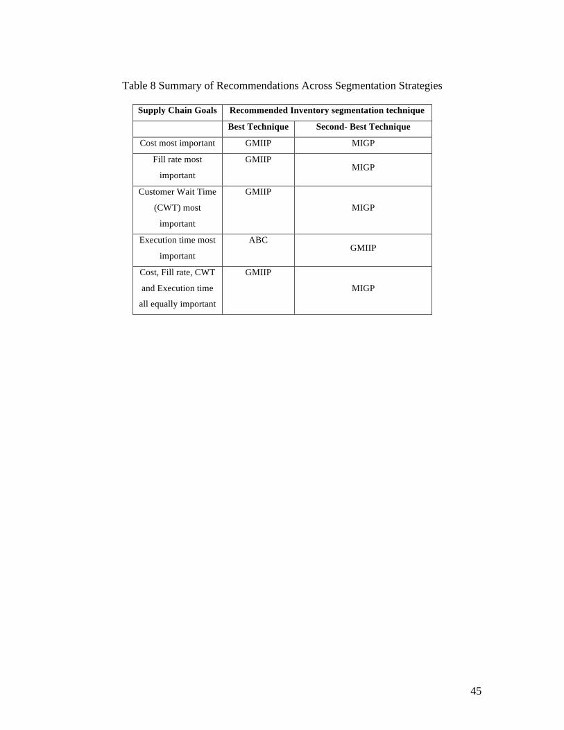
Table 8 summarizes the results based on the supply chain goals. These recommendations
are based on the results obtained by comparing the performance of these three techniques.
It is important to choose the right type of inventory segmentation methodology that suits
the goals of the supply chain under consideration. Also, the feasibility of using these
methods has to be evaluated. Hence we recommend the best and also the second best
inventory segmentation technique for the supply chain goals considered.
Table 8 placed near here
These recommendations can be used in combination with the recommendations to
choose the inventory segmentation technique. Thus a strategy can be developed that helps
to choose an inventory segmentation technique and further helps to arrive at a
recommended combination of factors in the inventory segmentation process. This can
help in finding an effective trade off between the managerial convenience and the loss of
identity in the process of inventory classification.
5 Summary and Future Work This paper presented techniques that can help achieve an effective trade off between the
managerial convenience and penalty cost in the inventory classification or segmentation

31
process. It is very important to state here that managerial convenience is a highly
subjective term and hence the results of an inventory segmentation process will depend
on the expectations of the manager. Because of this, the research recommends strategies
for inventory segmentation when different supply chain goals are important.
The primary focus of the work is in analyzing the impact of segmentation strategies
for large-scale, multi-item inventory systems. The basic idea is to segment or group the
items so that the items can be more easily managed, especially with regards to setting the
inventory policies for the items. Statistical clustering techniques were examined to
determine the effect of using different attributes within the clustering procedures and the
resulting performance of the inventory policy settings. A new data generation procedure
was developed and used to generate large-scale data sets for use during the experiments.
Two new approaches to the setting of the policies were developed and analyzed. The
Multi-Item Group Policy (MIGP) procedure sets a policy for the group of items, such that
all items in the group use the same policy parameters. This reduces the computations to
set the policies significantly, but also causes a lack of identity for the items and a
resulting lack of performance when compared to individual policy setting procedures.
The Group Multi Item Individual Policy (GMIIP) procedure uses the resulting groups to
set the policies of the individual items within the groups. This results in more
computation but policies that are significantly closer to individually determining the
policies for each item. The ABC approach to classifying the items was also compared to
the MIGP and GMIIP procedures. The experimental results show that the MIGP and the
GMIIP inventory segmentation techniques outperform conventional inventory
classification technique like ABC analysis both from the perspective of achieving cost as

32
well as service oriented goals of the supply chain. Given a specific target of penalty cost
and managerial convenience (preferred number of inventory groups to be managed) the
MIGP and GMIIP techniques hold the potential to achieve the desired performance
metrics for different types of inventory systems.
This research has established and tested a basic, generic framework to handle the
challenging task of inventory classification. There are many aspects of this framework
that can be further refined. In the MIGP and GMIIP inventory segmentation techniques,
the items are grouped and the policies are set (either individually or for the group). There
is a need to formulate an optimization model that combines the grouping and policy-
making processes at the same time. Such an optimization model may help to explicitly
capture the trade-offs between cost and service that result from the grouping processes.
Finally, the ideas within this paper could be extended to the application of segmentation
techniques on large-scale multi-item multi-echelon inventory systems, where the policy
setting process is significantly more complicated.
Acknowledgements Thanks to the anonymous reviewers for their suggestions to improve the article. This
material is based upon work supported by the National Science Foundation under Grant
No. 0437408. Any opinions, findings, and conclusions or recommendations expressed in
this material are those of the author(s) and do not necessarily reflect the views of the
National Science Foundation.

33
6 References 1. Al-Rifai´ M. H. and Rossetti, M. D. (2007), “An Efficient Heuristic Optimization
Algorithm for a Two-Echelon (R, Q) Inventory System”, International Journal of
Production Economics, Vol. 109, No. 1-2, pp. 195-213.
2. Caglar, D., Li, C-L. and Simchi-Levi, D. (2004), “Two-echelon spare parts inventory
system subject to a service constraint”, IIE Transactions, Vol. 36, pp. 655-666.
3. Chakravarty, A. (1981), “Multi-item inventory aggregation into groups”, Journal of
the Operational Research Society, Vol. 32, pp. 19-26.
4. Chu, C., Liang, G. and Liao, C. (2008), “Controlling inventory by combining ABC
analysis and fuzzy classification”, Computers & Industrial Engineering, Vol. 55, no.
4, pp. 841-851
5. Cohen, M. A., Kamesam, P. V., Kleindorfer, P., Lee, H., and Tekerian, A. (1990),
“Optimizer: IBM’s multi-echelon inventory system for managing service logistics”,
Interfaces, Vol. 20, No. 1, pp. 65-82.
6. Deshpande, V., Cohen, M.A., and Donohue, K. (2003), “An Empirical Study of
Service Differentiation for Weapon System Service Parts”, Operations Research,
Vol. 51, No. 4, pp. 518-530.
7. Deuermeyer, B. and Schwarz, L. B. (1981), “A Model for the Analysis of System
Service Level in Warehouse/ Retailer Distribution Systems: the Identical Retailer
Case”, in: L. B. Schwarz (Ed.), Studies in Management Sciences, Vol. 16, Multi-
Level Production/ Inventory Control Systems, North-Holland, Amsterdam, pp. 163-
193.

34
8. Ernst, R. and Cohen, M.A. (1986), “Operations Related Groups (ORGs): A
Clustering Procedure for Production / Inventory Systems”, Journal of Operations
Management, Vol. 9, No. 4, pp. 574-598.
9. Everitt, B.S., Landau, S., and Leese, M. (2001), Cluster Analysis, 4th edition, Oxford
University Press Inc., New York.
10. Gümüs, A. T. and Güneri, A. F. (2007), “Multi-echelon inventory management in
supply chains with uncertain demand and lead times: literature review from an
operational research perspective”, Proceedings of the Institution of Mechanical
Engineers, Part B: Journal of Engineering Manufacture, Vol. 221, No. 10, pp. 1553-
1570.
11. Hopp, W. J., Spearman, M. L., and Zhang, R. Q. (1997), “Easily implementable
inventory control policies”, Operations Research, Vol. 45, No. 3, pp. 327-340.
12. Hopp, W. J., Zhang, R. Q., and Spearman, M. L. (1999), “An easily implementable
hierarchical heuristic for a two-echelon spare parts distribution system”, IIE
Transactions, Vol. 31, pp. 977-988.
13. Lenard, J. and Roy, B. (1995), “Multi-item inventory control: a multi-criteria view”,
European Journal of Operational Research, Vol. 87, pp. 685-692.
14. Margulis, R. (2009), “Lowe’s, Whirlpool, Rite Aid, Kimberly-Clark, Wal-Mart,
eBizPrize, Schneider National, and Safeway Honored at 12th VICS Achievement
Awards”, VICS Press Release,
<http://www.vics.org/docs/KSurvey/press_releases/pdf/VICS_2009_Winners_Releas
e.pdf>, accessed 8/21/09.

35
15. Moore, R. and Cox, J. (1992), “An analysis of the forecasting function in large-scale
inventory systems”, International Journal of Production Research, Vol. 30, No. 9,
pp. 1987-2010.
16. Muckstadt, J. A., (2005), Analysis and Algorithms for Service Parts Supply Chains,
Springer Science+Media, Inc.
17. Partovi, F. Y. and Anandarajan, M. (2002), “Classifying inventory using an artificial
neural network approach”, Computers &Industrial Engineering, Vol. 41, No. 4, pp.
389-404
18. Ramanathan, R. (2006)., “ABC inventory classification with multiple criteria using
weighted linear optimization”, Computers and Operations Research, Vol.33 (3), pp.
695-700
19. Romesburg, H. C. (1984), Cluster Analysis for Researchers, 1st edition, Lifetime
Learning Publications, California.
20. Silver, E. A., Pyke, D. F., and Peterson, R. (1998), Inventory Management and
Production Planning and Scheduling, 3rd edition, John Wiley & Sons, New York.
21. Svoronos, A and Zipkin, P. (1988), “Estimating the performance of multi-level
inventory systems”, Operations Research, Vol. 36, No. 1, pp. 57-72.
22. Williams, B. D. and Tokar, T. (2008), “A review of inventory management research
in major logistics journals – Themes and future directions”, The International Journal
of Logistics Management, Vol. 19, No. 2, pp. 212-232.
23. Zhou, P. and Fan, L. (2007), “A note on multi-criteria ABC inventory classification
using weighted linear optimization”, European Journal of Operational Research,
Vol. 182, pp. 1488-1491.

36
24. Zipkin, P. H. (2002), Foundations of Inventory Management, McGraw-Hill
Companions, Inc.

37
Table 1 Inventory system characteristics
Inventory system type Item attributes Repairable Consumable Repairable and Consumable Unit cost ($) High Low Medium Average annual demand (units) Low High Medium
Replenishment lead time (days) High Low Medium
Mean lead time demand (units) Low High Medium
Variance of lead time demand High Low Medium
Desired fill rate High Medium Medium Essentiality High Medium Medium Criticality High Medium Medium Item size High Low Medium Item weight High Low Medium

38
Table 2 Quantification of attribute value categories Category values
Low Medium High Item attributes Range Low
Range Low
Range Low
Range High
Range Low
Range High
Unit cost ($) 1 10,000 10,000 50,000 50,000 100,000 Average annual demand (units) 1 10,000 10,000 25,000 25,000 50,000
Replenishment lead time (days) 1 5 5 10 10 20
Mean lead time demand (units) Derivable Derivable Derivable Derivable Derivable Derivable
Variance of lead time demand Derivable Derivable Derivable Derivable Derivable Derivable
Desired fill rate 70 80 80 90 90 95 *Essentiality 3 2 2 2 2 1 *Criticality 3 2 2 2 2 1 *Size 3 2 2 2 2 1 *Weight 3 2 2 2 2 1 *Note: The category values for the attributes essentiality, criticality, size and weight have the following meaning: 1 = high, 2 = medium, 3 = low.

39
Table 3 Example Strata for Generating Datasets % of Total
Average annual Demand
Lead Time Cost Var-Annual Demand
Var-Lead time
Essentiality
33% [5000-10000] H [1-5] L -80% [1-5] L -80%
[500-1000] H-80%
[0-2.5] L -80%
[1] H-33%
[10-15] H-10%
[25-50] H-10%
[100-500] M-10%
[5-10] H-10%
[2] M-33%
[5-10] M-10% [5-25] M-10%
[0-100] L -10% [2.5-5] M-10%
[3] L-33%
33% [1000-5000] M [5-10] M-80% [5-25] M-80%
[100-500] M-80%
[2.5-5] M-80%
[1] H-33%
[1-5] L -10% [1-5] L -10%
[0-100] L -10% [0-2.5] L -10%
[2] M-33%
[10-15] H-10%
[25-50] H-10%
[500-1000] H-10%
[5-10] H-10%
[3] L-33%
33% [1-1000] L [10-15] H-80%
[25-50] H-80%
[0-100] L -80% [5-10] H-80%
[1] H-33%
[5-10] M-10% [5-25] M-10%
[500-1000] H-10%
[2.5-5] M-10%
[2] M-33%
[1-5] L -10% [1-5] L -10%
[100-500] M-10%
[0-2.5] L -10%
[3] L-33%

40
Table 4 Summary of Screening Experimental Results
Consumable Repairable Factors PC ET FR CWT PC ET FR CWT Number of clusters - + + + - + + + Clustering algorithm + - + Group policy deciding criteria + + + - + Unit cost - - + + Average annual demand - + + Replenishment lead-time + + + Mean lead time demand + - - - Variance of lead time Desired fill rate Essentiality Criticality - Item size - Item weight +

41
Table 5 Factors and Levels for Combined Response Experiments Factors Levels Number of clusters 10%, 20%, 30%, 40%, 50%, 60%, 70%, 80% Group Policy Criterion Mean, median, minimum, maximum Clustering Algorithm UPGMA, Ward’s

42
Table 6 General Recommendations Based on Response Surface Analysis
Supply Chain Goals
Attributes to be
included in the
clustering process
Number of inventory groups Clustering
Algorithm
Group Policy
criteria
Cost most important High (60-70% of the total
number of items) UPGMA Minimum
Fill rate most important High (60-70% of the total
number of items) UPGMA Maximum
Customer Wait Time
(CWT) most important
High (60-80% of the total
number of items) UPGMA Maximum
Execution time most
important
Low (10-20% of the total
number of items) UPGMA Mean
Cost, Fill rate, CWT and
Execution time all equally
important
Unit Cost
Lead Time
Mean Lead time
demand
Essentiality
Criticality
Size Moderate (30-40% of the total
number of items) UPGMA Mean

43
Table 7 Percentage above the MIIP value for MIGP, GMIIP, and ABC Analysis Penalty Cost Fill Rate Customer Wait Time
Size MIGP ABC GMIIP MIGP ABC GMIIP MIGP ABC GMIIP
2 25.48 39.50 3.29 22.329 53.531 1.086 23.40 45.68 1.56
4 31.79 44.70 3.44 22.782 54.841 1.086 23.80 52.70 1.70
6 34.36 47.18 3.96 23.505 55.073 1.086 24.52 57.08 1.71
8 38.24 51.28 4.79 24.572 55.045 1.086 25.00 59.20 1.80
10 40.14 55.14 5.05 24.723 55.439 1.087 26.34 63.44 1.89

44
Figure 1: Execution Time (Seconds) for Segmentation Techniques
45
Table 8 Summary of Recommendations Across Segmentation Strategies
Supply Chain Goals Recommended Inventory segmentation technique
Best Technique Second- Best Technique
Cost most important GMIIP MIGP
Fill rate most
important
GMIIP MIGP
Customer Wait Time
(CWT) most
important
GMIIP
MIGP
Execution time most
important
ABC GMIIP
Cost, Fill rate, CWT
and Execution time
all equally important
GMIIP
MIGP
Recommended