Evaluation of graphical and multivariate statistical methods for classification of water chemistry data

Ciineyt Giiler · Geoffrey D. Thyne · John E. McCray A. Keith Turner

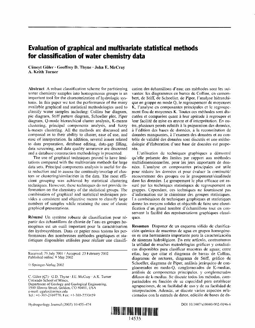
Abstract A robust classification scheme for partitioning water chemistry samples into homogeneous groups is an important tool for the characterization of hydrologic sys­tems. In this paper we test the performance of the many available graphical and statistical methodologies used to classify water samples including: Collins bar diagram, pie diagram, Stiff pattern diagram, Schoeller plot, Piper diagram, Q-mode hierarchical cluster analysis, K-means clustering, principal components analysis, and fuzzy k-means clustering. All the methods are discussed and compared as to their ability to cluster, ease of use, and ease of interpretation. In addition, several issues related to data preparation, database editing, data-gap filling, data screening, and data quality assurance are discussed and a database construction methodology is presented.

The use of graphical techniques proved to have limi­tations compared with the multivariate methods for large data sets. Principal components analysis is useful for da­ta reduction and to assess the continuity/overlap of clus­ters or clustering/similarities in the data. The most effi­cient grouping was achieved by statistical clustering techniques. However, these techniques do not provide in­formation on the chemistry of the statistical groups. The combination of graphical and statistical techniques pro­vides a consistent and objective means to classify large numbers of samples while retaining the ease of classic graphical presentations.

Resume Un systeme robuste de classification pour re­partir des echantillons de chimie de l'eau en groupes ho­mogenes est un outil important pour Ia caracterisation des hydrosystemes. Dans ce papier nous testons les per­formances des nombreuses methodes graphiques et sta­tistiques disponibles utilisees pour realiser une classifi-

Received: 25 .July 2001 I Accepted: 23 February 2002 Published online: 9 May 2002

!tl Springer-Verlag 2002

C. Guier (0) · G.D. Thyne · J.E. McCray · A.K. Turner Colorado School of Mines, Department of Geology and Geological Engineering, 1500 11linois Street, Golden, CO 8040 L USA e-mail: cguler@rnines.edu Tel.: + 1-303-2)69770. Fax: + I-303-2733X59

Hydrogeology Journal (2002) I 0:455-474

cation des echantillons d'eau; ces methodes sont les sui­vantes: les diagrammes en barres de Collins, en camem­bert, de Stiff, de Schoeller, de Piper, !'analyse hierarchi­que en grappe en mode Q, le regroupement de moyennes K, !'analyse en composantes principales et le regroupe­ment flou de moyennes K. Toutes ces methodes sont dis­cutees et comparees quant a leur aptitude a regrouper et leur facilite de mise en reuvre et d'interpretation. En ou­tre, plusieurs points relatifs a la preparation des donnees, a !'edition des bases de donnees, a la reconstitution de donnees manquantes, a l'examen des donnees et au con­trole de validite des donnees sont discutes et une metho­dologie d'elaboration d'une base de donnees est propo­see.

L'utilisation de techniques graphiques a demontre qu'elle presente des limites par rapport aux methodes multidimensionnelles, pour les jeux importants de don­nees. L'analyse en composantes principales est utile pour reduire les donnees et pour evaluer Ia continuite/ recouvrement des groupes ou le groupement/similitude dans les donnees. Le groupement le plus efficace est as­sure par les techniques statistiques de regroupement en grappes. Cependant, ces techniques ne fournissent pas d'information sur le chimisme des groupes statistiques. La combinaison de techniques graphiques et statistiques donne les moyens solides et objecti£.;; de faire une classi­fication d'un grand nombre d'echantillons tout en con­servant Ia facilite des representations graphiques classi­ques.

Resumen Disponer de un esquema solido de clasifica­ci6n quimica de muestras de agua en grupos homogene­os es una herramienta importante para la caracterizaci6n de sistemas hidrol6gicos. En este articulo, contrastamos la utilidad de muchas metodologias gnificas y estadisti­cas disponibles para clasificar muestras de aguas; entre elias, hay que citar el diagrama de barras de Collins, diagramas de sectores, diagrama de StitT, gnifico de Schoeller, diagrama de Piper, analisis jerarquico de con­glomerados en modo-Q, conglomerados de K-medias, analisis de componentes principales, y conglomerados difusos de k-medias. Se discute todos los metodos, com­parandolos en funcion de su capacidad para establecer agrupaciones, de su facilidad de uso y de su facilidad de interpretacion. Ademas, se discutc varios aspectos rela­cionados con Ia entrada de datos, edici6n de bases de da-

DOl I 0.1 007/s I 0040-002-0196-6

111111111111 11111111111111111111111 14535

456

tos, extrapolaci6n de datos en series incompletas, visua­lizaci6n de datos, y garantia de calidad de los datos, y se presenta una metodologia para elaborar una base de da­tos.

Se demuestra que el uso de tecnicas graticas padece limitaciones respecto a los metodos multivariados para conjuntos de datos numerosos. El amilisis de componen­tes principales es uti! para reducir el numero de datos y establecer Ia continuidad/superposici6n de grupos o agrupaciones/similaridades en los datos. Los resultados mas efectivos se logran mediante tecnicas estadisticas de agrupamiento; sin embargo, estas no proporcionan infor­macion sobre Ia quimica de los grupos estadisticos. La combinaci6n de tecnicas graficas y estadisticas posibilita un enfoque coherente y objetivo para clasificar numeros elevados de muestras y, a Ia vez, mantener Ia facilidad de las presentaciones graficas convencionales.

Keywords Classification techniques · Cluster analysis · Database construction · Fuzzy k-means clustering · Water chemistry

Introduction

The chemical composition of surface and groundwater is controlled by many factors that include composition of precipitation, mineralogy of the watershed and aquifers, climate, and topography. These factors combine to create diverse water types that change spatially and temporally. In our study area, which lies within the south Lahontan hydrologic region of southeastern California (Fig. 1 ), there is a wide variety of climatic conditions (high alpine to desert), hydrologic regimes (alluvial basin-fill aqui­fers, fractured rock aquifers, and playas) and geologic environments (igneous rocks, volcanic rocks, metamor­phic rocks, sedimentary deposits, evaporites, and miner­alized zones). Thus, the samples from the area could po­tentially represent a variety of water types providing an opportunity to test the performance of many of the avail­able graphical and statistical methodologies used to clas­sify water samples.

The use of major ions as natural tracers (Back 1966) has become a very common method to delineate flow paths in aquifers. Generally, the approach is to divide the samples into hydrochemical facies (aka water types), that is groups of samples with similar chemical characteris­tics that can then be correlated with location. The spatial variability observed in the composition of these natural tracers can provide insight into aquifer heterogeneity and connectivity, as well as the physical and chemical pro­cesses controlling water chemistry. Thus, a robust classi­fication scheme for partitioning water chemistry samples into homogeneous groups can be an important tool for the successful characterization of hydrogeologic sys­tems. A variety of graphical and multivariate statistical techniques have been devised since the early 1920s in order to facilitate the classification of waters, with the ultimate goal of dividing a group of samples into similar

Hydrogeology Journal (2002) 10:455-474

124'

State of CALIFORNIA

1110

120.

Fig. 1 Location of the study area

NC. North Coast SF • San Francisro Bay CC- Cootml Coii$1 sc • South Coast SR • Sacramento River SJ • San Joaquin River TL - TUlare Lake Nl· North Lahontan SL - South Lahontan CR- Colorado River

homogeneous groups (each representing a hydrochemi­cal facies). Several commonly used graphical methods and multivariate statistical techniques are available in­cluding: Collins bar diagram, pie diagram, Stiff pattern diagram, Schoeller semi-logarithmic diagram, Piper diagram, Q-mode hierarchical cluster analysis (HCA), K-means clustering (KMC), principal components analy­sis (PCA), and fuzzy k-means clustering (FKM). This paper utilizes a relatively large data set to review these techniques and compare their ease of use and ability to sort water chemistry samples into groups.

Hydrogeologic Setting The study area is part of the Basin and Range Province of the southwestern USA and extends from 35-3T of latitude north and from 117-118.5° of longitude west (Fig. 1). The area comprises a portion of the Sierra Ne­vada mountain range, which is the recharge area, and ad­joining alluvial basins, which are arid. Because of the modem arid climate, surface water is scarce in the area and groundwater is the only source of drinking and household use water (Berenbrock and Schroeder 1994). Thus, effective management of the groundwater resourc­es requires an accurate model for the aquifer characteris­tics, groundwater flow directions, recharge mechanisms, discharge mechanisms, and water chemistry processes.

In the basin and range groundwater system, water flows from recharge areas in the mountains to discharge areas in the adjacent valleys (Maxey 1968). This local flow system is often modified by local geologic, physio-

DO 1 I 0.1 007 Is I 0040-002-0 I 96-6

graphic, and climatic factors. During the Pleistocene and Holocene epochs, the valley floors in the study area were periodically occupied by a chain of lakes stretching from Mono Lake in the north to Lake Manley in Death Valley (Duffield and Smith 1978; Lipinski and Knochenmus 1981 ). Present-day valley floors are occupied by playas, known in different localities as "salt lakes," "soda lakes," "alkali marshes," "dry lakes," or "borax lakes", where the majority of groundwater discharges by evapo­transpiration (Lee 1912; Fenneman 1931; Dutcher and Moyle 1973 ). Minor discharge also occurs by other ways including discharge from springs, seeps, and pumping from wells. The groundwater in the area occurs in two porosity regimes: (I) intergranular porosity found mostly in alluvial basin-fill aquifers, and (2) fracture porosity found in the mountain watersheds. The alluvial basin-fill aquifers can be further divided into two components: a shallow saline aquifer (<!50 m depth), and a deep ( 610 m), locally confined aquifer that extends throughout the area (Dutcher and Moyle 1973 ).

Methods

The available major solute data (spring, surface, and well water) for the area was compiled for this study in order to create a comprehensive database, called SLH­DATA (south Lahontan hydrochemical database), for the

Table 1 Data sources used to create the SLHDATA database. Code Data sources NWIS: US Geological Survey number National Water Storage and Retrieval System

I Barnes et a!. ( 1981) 2 Berenbroek ( 1987)

457

classification of waters into hydrochemical facies repre­senting "water types". The data were arranged in rows (for sampling locations) and in columns (for chemical parameters). The entire database consists of chemical an­alyses of !52 spring samples, 153 surface samples, and 1,063 well (groundwater) samples, including temporal samples (samples collected over a period of time at the same location). Sources of the data are presented in Table 1. In the case of multiple samples from the same location, the more recent and/or the more complete sam­ple data were included in the statistical analysis unless evaluation of temporal effects was desired. Database construction procedures and comparison of the results from the various statistical and graphical techniques is discussed in detail in the following sections. Detailed analysis of the graphical and statistical water groups in terms of the physical and chemical factors that control water chemistry is not the focus of this paper. Instead, we are interested here in the ability of available tech­niques to classify a diverse set of samples into distinct groups.

Of the 39 hydrochemical variables (consisting of ma­jor ions, minor ions, trace elements, and isotope data) in the compiled database, 11 variables (specific conduc­tance, pH, Ca, Mg, Na, K, Cl, S04, HC03, Si02, and F) occur most often and, thus, were used in our evaluation. It is usually assumed that adequate quality assurance (QA) and quality control (QC) measures were performed

Number of samples

Surface Spring Well

194 3 Berenbrock and Schroeder ( 1994) 108 4 8 uono and Packard ( 1982) 3 5 California State University, Bakersfield, unpublished data 51 38 74 6 Dockter ( 1980a) I 7 Dockter ( 1980b) 2 8 Feth eta!. ( 1964) I 9 Font ( 1995) 3 18

10 Fournier and Thompson ( 1980) 8 3 II Hollett et al. (1991) 5 12 Houghton (1994) 10 2 25 13 Hunt et al. (1966) I 14 Johnson ( 1993) 13 15 Johnson et al. ( 1991) 6 16 Lamb ct al. (1986) 42 17 Lopes ( 198 7) 14 14 18 Maltby et al. ( 1985) 45 19 McHugh et al. ( 1981) 70 8 20 Melack et al. ( 1985) 10 21 Miller ( 1977) 2 7 2 22 Moyle ( 1963) I 137 23 Moyle ( 1969) 24 96 24 Moyle (1971) 57 25 Ostdick ( 1997) 6 14 14 26 Robinson and Beetem ( 1975) I 27 US Bureau of Reclamation ( 1993) 33 28 US Geological Survey NWIS QW data 28 154 29 Whelan et al. ( 1989) I 9 30 No source information available 3 8

Hydrogeology Journal (2002) I 0:455-474 DOl I 0.1 007/sl 0040-002-0196-6

458

at the time of original data collection and analysis; how­ever, we screened the data to verify that they were usable (see below for further discussion). The data collection methods, which are similar are described in detail for most of the data sources, or documented in US Geologi­cal Survey's "Techniques of water-resources investiga­tions" manuals (e.g., Brown eta!. 1970; Wood 1981).

The Statistica Release 5.0 (StatSoft, Inc. 1995) com­mercial software package was utilized for the basic sta­tistical analyses performed. Microsoft Excel 97 (Micro­soft Corporation 1985) and RockWorks (RockWare, Inc. 1999) were used for the graphical analyses. Classifica­tion of the data was also performed using FuzME (Fuzzy k-Means with Extragrades; Minasny and McBratney 1999). The techniques used include cluster analysis (HCA and KMC), principle components analysis (PCA), fuzzy k-means clustering (FKM), and a variety of graph­ical methods. Detailed technical descriptions of HCA, KMC, and PCA techniques and a description of the FKM technique are provided in StatSoft, Inc. ( 1997) and Bezdek eta!. ( 1984 ), respectively.

Database Editing Figure 2 is a flow chart that summarizes the methodolo­gy used for compiling the hydrochemical database. If re­ported, field measurements of alkalinity and pH were used for the construction of the database. Otherwise, lab­oratory measurements of these variables were used. Some of the individual data sets contained the same sam­ple, or apparent near-duplicate analyses for minor ele­ments. In general, there were more discrepancies for iron than for any other minor element. This was probably be­cause of the different ways in which iron concentrations were expressed, or the convention being used was not clearly stated. We have chosen not to use any minor ele­ment data for our study because of these sorts of prob­lems.

Samples with uncertain locations were located using reports and maps or eliminated from the database when such information was not available. Locations of sites that had only the name of the well or spring were deter­mined as accurately as possible, usually to several hundred meters and always within 1 km. Well-water samples without sampling depths were retained in the database, but eliminated from the multivariate statistical analysis.

Units of measurement were sometimes inconsistent between different data sets. All values were converted to an internally consistent format (all units are in mg L-1 in the SLHDATA database). Common reporting units for data sets were weight-per-volume units [milligrams per liter (mg L-1) and micrograms per liter (!lg L-1)], equiva­lent-weight units [milliequivalents per liter (meg L-1) and microequivalents per liter (11eq L-1)], or weight-per­weight units [parts per million (ppm), parts per billion (ppb ), and parts per trillion (ppt)]. Conversion factors for calculation of a unit from the other units are given by Hem (1989).

Hydrogeology Journal (2002) 10:455-474

Combined Database (SLHDATA)

Database Editing Procedures - lil.lJJl!~a!l· n:ni(n til . Near-duphcate records - Uncertain sample locations - Unccnam sampling depths llhr \\ell>< .I - Different unit reponing fnrmats

CctH<>I\.xl values ~ V,;thJ\!S' 4d.ecfinn hmh {icss-thilrt \a~ues) • \·ah.h:~'-i.ll!tecti-on limit ~·gn.~al~f·lh~m values)

I Data-Gap Filling Procedures - Com;-latinn ana!~sis - Esti mutlon of mi ssmg ndues

• Snnpl~ lin<'"f ~e.r.:"i' 111

• C~CtKik~mic:d r.:latH~rr~h1 r~

L ···. FLAG · J

Calcnla~ ll1ld El!tirnated Valttes

IMPORT Into Statistical i

' Software Package

Calculate Charge Balance

Errors

!.>iscard llnbnhHK't~d

Sllmplcs

! Data ('harnl'tcrization & Scrccnin~ j · 1 )c~~tilzlJ\~: $\;;li:<li\;> I

- (.'~ntraJ h.'ntkn..:-j inh.'rtH. mi'd~<-tH. mt,, . .h~) I - JJ!'P"1'1•>r• (s!andard d.::v•~li'''L ,;;,"11'''1 I

(,rtlpbtcnl Displ;lYS

- lli:'\1ogram~~ S,..:-:tdh'rph~H. Pn)h;,tblhty ph.~~

Fig. 2 Methodology used for compiling and editing the SLHDATA database

Censored values Water chemistry data are frequently censored, that is, con­centrations of some elements are reported as non­detected, less-than or greater-than. These values are created by the lower or upper detection limit of the instrument or method used. Censored data are not appropriate for many multivariate statistical techniques. Therefore, the non-de­tected, less-than, and greater-than values must be replaced with unqualified values (Farnham et a!. 2002). In our dat­abase there were no censored values for the 11 variables used in this study, however, because this is often not the case we briefly discuss methods to deal with this situation.

DOl 10.1007 /s 10040-002-0196-6

A number of techniques have been suggested for re­placement of a censored value including replacement of the less-than values by 3/4 times the lower detection lim­it and the greater-than values by 4/3 times upper detec­tion limit (VanTrump and Miesch 1977). An alternative is replacement of less-than values by 0.55 times the low­er detection limit and the greater-than values by 1.7 times upper detection limit (Sanford et al. 1993). For da­ta where the proportion of the censored values is > 10%, another method that was devised by Sanford eta!. ( 1993) can be used. This method estimates the mean of the nor­mal distribution using a maximum likelihood estimation method. Then, this estimated mean is used to derive an estimated replacement value.

Data-gap filling procedures -estimation of the missing values Usually the effective use of many of the methods re­quires complete water analyses (no missing data values). Missing data values may make the use of graphical water chemistry techniques impossible, or limit the quality of the statistical analysis. During the statistical analysis, most statistical software packages replace those missing values with means of the variables, or prompt the user for case-wise deletion of analytical data, both of which are not desirable. This can bias statistical analyses if these values represent a significant number of the data being analyzed.

Table 2 Charge balance (CB) Code no." Years collected statistics for the individual data

sources I 1981 2 1977-1984 3 1987-1989 4 1968-1980 5 1994-1998 6 1978 7 1978 8 1959 9 1989-1994

10 1974-1979 II 1945-1978 12 1993-1994 13 Unknown 14 1993 15 1990 16 1986-1991 17 1986 18 1984-1985 19 1979 20 1982 21 1967-1972 22 1917-1960 23 1917-1967 24 1916-1969 25 1996

a Data sources corresponding 26 1965 to code numbers arc listed in 27 1990-1992 Table I. The+ and- columns 28 1945-1990 refer to the number of analyses 29 1976-1987 from a data source having posi- 30 1989-1996 tive and negative CB errors

Hydrogeology Journal (2002) I 0:455--4 74

459

There are statistical methods and chemical relationships that can be employed to estimate missing data values. For instance, missing conductance data can be calculated from total dissolved solids (TDS) data by using a simple linear regression method. In our database, a significantly (p<O.OOl) high correlation coefficient (r-=0.984) was found to exist between these two variables. The p-value is the significance probability for testing the null hypothesis that true correlation in the population is zero. A small value of p (e.g., p<O.OO I) indicates that there is a significant corre­lation. Thus, missing potassium (K) values were estimated by utilizing the linear relationship between potassium and sodium (Na), which had a significantly (p<O.OOl) high cor­relation coefficient of0.904.

Missing bicarbonate (HC03) data can be calculated from alkalinity values and pH. Inverting the problem, missing pH values can be calculated by using Eq. (1) if the C03 and HC03 values were reported:

[co~ J . w-pH

K~ = ..>o-----,----"--c;---~ [HC03 )

(1)

The same relationship can also be used to calculate the missing carbonate (C03) values if pH was reported. Fi­nally, if there were no means of establishing a value, a value of "-9,999" was entered for the missing value, in­dicating that no data were available for that entry. In our data set there were very few (3%) samples with censored or missing values.

+ CB error range Median Mean (±I cr)

I 0 -1.04 -1.04 -1.04 (±0.00) 82 112 -10.31 7.75 0.35 0.16(±2.87) 54 54 -9.43 8.66 -0.11 0.24 (±3.95)

2 I -2.05 0.96 -1.31 -0.80 (±1.57) 61 102 -9.44 10.04 1.33 1.88 (±3.73)

0 I 0.32 0.32 0.32 (±0.00) I I -0.02 0.52 0.25 0.25 (±0.38) I 0 -1.14 -1.14 -1.14(±0.00)

14 7 -3.70 3.03 -1.25 -0.83 (±2.01) 7 5 -5.71 9.41 -0.30 0.82 (±4.31) I 4 -0.12 5.30 1.69 2.03 (±2.15)

12 25 -8.39 10.40 0.87 0.90(±4.01) 0 I 0.34 0.34 0.34 (±0.00) 9 4 -8.94 8.16 -1.43 -1.04 (±4.34) 4 2 -3.30 8.33 -0.28 0.56 (±4.34)

34 8 -5.14 2.05 -2.20 -1.82 (±1.80) 10 18 -2.65 10.39 0.84 1.35 (±2.92) 30 15 -6.02 8.51 -0.86 -0.92 (±2.97) 64 14 -9.45 9.10 -5.00 --4.02 (±4.38)

7 3 -6.17 4.75 -2.68 -2.01 (±3.56) 4 7 -2.31 4.67 0.79 0.89 (±2.02)

28 110 -2.34 10.13 0.13 1.13 (±2.23) 17 103 -9.55 8.74 1.89 2.00 (±2.28) 22 35 ~-3.81 8.84 0.20 0.74 (±1.94) 17 17 -8.70 10.32 0.03 1.14 (±5.32)

I 0 -().09 -0.09 -0.09 (±0.00) 8 25 -3.13 6.88 2.38 1.99 (±2.55)

119 63 -8.10 9.92 -0.94 -0.75 (±2.69) I 9 -0.76 9.99 6.54 5.18 (±3.52) 3 8 -10.04 9.58 2.59 2.35 (±5.63)

DO I I 0.1 007 /s I 0040-002-0196-6

460

Fig. 3 Distribution of percent charge balance error for a, b spring, c, d well, and e. f sur­face water samples

Charge balance error

Surl&:-e Water

The edited chemical analyses in the SLHDATA database were tested for charge balance (Freeze and Cherry 1979):

Iz·mc- Iz ·nla %Charge Balance (CB) Error= · 100 (2)

Iz·mc+ Iz·ma

where z is the absolute value of the ionic valence, me the molality of cationic species and ma the molality of the anionic species. Conventions and assumptions used in balancing the analyses included:

I. When bicarbonate and carbonate data were not given, alkalinity, if available, was used to estimate a bicar­bonate concentration.

Hydrogeology Journal (2002) 10:455-4 74

,····:·.,·,::-·····

32::' d)

3C·'

IS

~' t6l & !4,

&: 12\ w: s: 6'

4'

(l

lli•togrom of l'erc.ml. (%) CharS" llillUk'<' FtrM {Spring Water)

Sample N 152 Mean :ft612 l\-ledian : 0.181 Std Dev. : :UO(, SktWIICM! : 0.035

IH~Wg,ntm of !'ere-em ("'•) Charge Balllnue FJTor (Well Water)

Sample N : 1063 ~kiln · ll.,28 MediN~ : (l !68 Sld .. IX'I. : 3.203 Skcwne~~ : 0.:128

Hi•1ogram <>fl'crcon1 (~i1) Cllarg:e Tl.!llanc< Err<tr (St .. fnce Water)

.]1 .;., .jf ,(; 4 .: ()

2. In the few cases where the calcium and magnesium data were missing, hardness was used to estimate the sum of calcium and magnesium concentrations.

Calculated charge balance errors are less than or equal to ±10.4% for SLHDATA database, which is an acceptable error for the purpose of this study {Table 2). Samples with errors greater than ±I 0.4% were not used. For the spring-water and well-water (groundwater) data, errors are evenly distributed between positive and negative values, and, thus, are not systematic (Fig. 3a-d). The charge balance errors of the surface water data showed a bimodal distribution and had a skewed distribution (Fig. 3e, f). Accordingly, the surface water samples were further studied. The samples were split into those from

DOl I 0.1007 Is 10040-002-0196-6

Fig. 4 Map view of HCA­derived subgroup and group values for the spring water samples

the Sierra Nevada mountain block and the Indian Wells­Owens Valley area (see Fig. 4 for locations). The Indian Wells-Owens Valley area samples have charge balance errors that approach a norn1al distribution and range from -6% to+ 10%, whereas the Sierra Nevadan samples had a strongly skewed distribution. The Sierra Nevada data included 78 samples collected for the Domeland Wilderness study (McHugh et al. 1981 ), which were identified as the source of the skewed distribution and indicates a systematic error in that particular set of ana­lyses. However, the error is not sufficient to remove the data set from the database.

Data screening The purpose of data screening is to evaluate the distri­bution characteristics of each variable in the database.

Hydrogeology Journal (2002) I 0:455-4 74

0

461

117"00'

EXPLAlVA TrON

Group I

f.}:~;J Group fi

~~ L"~~·

Gmupm

01• Spring sam ph: location wilh subgroup number

•4

N

+

We used univariate and bivariate statistical methods to assess each variable independently, and the relationship between variable pairs. The physical and chemical properties were evaluated using central tendency (mean, median, mode) and dispersion (standard devia­tion, skewness), and by graphical displays such as his­tograms, scatter plots, probability plots, and box plots. Based on these analyses, decisions were made concern­ing the need for, and selection of, appropriate transfor­mations to achieve a better approximation of the nor­mal distribution. This is important because most of the statistical analyses assume that data are normally dis­tributed.

The data screening showed that the data used in this study were universally skewed positively; the data con­tained a small number of high values. Most naturally oc­curring element distributions follow this pattern (Miesch

DOl 10.1007/sl0040-002-0196-6

462

1976). The data were log-transformed (except for pH) so that they more closely corresponded to normally distrib­uted data. Then, all the 11 variables were standardized by calculating their standard scores (z-scores) as follows:

x;-x Z.i ==

.1' (3)

where z;= standard score of the sample i; x;= value of sample i; i= mean; s= standard deviation.

Standardization scales the log-transformed data to a range of approximately -3 to +3 standard deviations, centered about a mean of zero. In this way, each variable has equal weight in the statistical analyses. Otherwise, the Euclidean distances will be influenced most strongly by the variable that has the greatest magnitude (Judd 1980; Berry 1995). Besides normalizing and reducing outliers, these transformations also tend to homogenize the variance of the distribution (Rummel 1970). The raw data (with data-gaps filled) were used for the graphical analyses, whereas the transformed (log-transformed and standardized) data were used for the hierarchical cluster analysis (HCA), K-means cluster analysis (KMC), prin­cipal components analysis (PCA), and fuzzy k-means clustering (FKM).

Results

The fundamental aim of the techniques compared here is to identify the chemical relationships between water samples. Samples with similar chemical characteristics often have similar hydrologic histories, similar recharge areas, infiltration pathways, and flow paths in terms of climate, mineralogy, and residence time. Table 3 shows

the various techniques and the required input data. For brevity, only the 152 spring water samples are discussed in the following text. The other subsets of the complete database produced similar results. A preliminary analy­sis of temporal effects, based on examination of individ­ual analyses, suggested that relatively little change oc­curred in the water quality of samples with time. This indicates that the spatial variability is the most impor­tant source of variation in the data, rather than the tem­poral factor. This conclusion was later tested and con­firmed as discussed in the statistical methods section. For that reason, we did not include samples from tempo­ral series to statistical analysis. This reduced the total number of samples to 118.The fundamental aim of the techniques compared here is to identify the chemical re­lationships between water samples. Samples with simi­lar chemical characteristics often have similar hydrolog­ic histories, similar recharge areas, infiltration path­ways, and flow paths in terms of climate, mineralogy, and residence time. Table 3 shows the various tech­niques and the required input data. For brevity, only the 152 spring water samples are discussed in the following text. The other subsets of the complete database pro­duced similar results. A preliminary analysis of tempo­ral effects, based on examination of individual analyses, suggested that relatively little change occurred in the water quality of samples with time. This indicates that the spatial variability is the most important source of variation in the data, rather than the temporal factor. This conclusion was later tested and confirmed as dis­cussed in the statistical methods section. For that rea­son, we did not include samples from temporal series to statistical analysis. This reduced the total number of samples to 118.

Table 3 Statistical and graphical techniques evaluated for the classification of water samples

Method Cations used Anions used

Cluster analysis All major, minor All major, minor (HCA and KMC) and trace elements and trace elements

Principal All major, minor All major, minor components and trace elements and trace elements analysis (PCA)

Fuzzy k-means All major, minor All major, minor Clustering (FKM) and trace elements and trace elements Piper diagram Na+ K, Ca, Mg Cl, S04,

HC03 + C03

Collins bar Na+ K, Ca, Mg Cl, S04, HC03 diagram (or HC03 + C03)

Pie diagram Na+ K, Ca, Mg Cl, S04, HC03

Stiff pattern Na (or Na + K), Cl, S04,

diagram Ca, Mg Fe HC03 co3 (optional) (optional)

Schoeller Na+ K, Ca, Mg CL S04, HC03 semi-logarithmic diagram

Chernotf faces Up to 20 parameters can be plotted

Hydrogeology Journal (2002) 10:455--474

Other parameters

All applicable parameters Yes (I) or no (0) statements, discrete variables

All applicable parameters Yes (I) or no (0) statements, discrete variables

Same as above

n/a

n/a

n/a

n/a

n/a

Input data and plotting units

Input: z-scores of the log-transformed data Output: distance matrix (KMC) and dendogram (HCA)

Input: z-scores of the log-transformed data Output: PCA scores

Input: same as above matrix Output: membership Relative %meq L-1

Relative %meq L-1 or meq L I

Relative %meq L -1

meq L-1

meq L -I in log-scale

meq L-1 or mg L-1 Other parameters in their respective units

DOl I 0.1 007/s I 0040-002-0196-6

463

PIPER DIAGRAM

Fig. 5 Piper diagram of the 118 spring water samples

Graphical Methods Most of the graphical methods are designed to simulta­neously represent the total dissolved solid concentration and the relative proportions of certain major ionic spe­cies (Hem 1989). All the graphical methods use a limited number of parameters, usually a subset of the available data, unlike the statistical methods that can utilize all the available parameters. The Piper diagram (Piper 1944; Fig. 5) is the most widely used graphical form and it is quite similar to the diagram proposed by Hill (1940, 1942). The diagram displays the relative concentrations of the major cations and anions on two separate trilinear plots, together with a central diamond plot where the points from the two trilinear plots are projected. The central diamond-shaped field (quadrilateral field) is used to show overall chemical character of the water (Hill 1940; Piper 1944 ). Back ( 1961) and Back and Hanshaw (1965) defined subdivisions of the diamond field, which

Hydrogeology Journal (2002) 10:455-474

represent water-type categories that form the basis for one common classification scheme for natural waters. The mixing of water from different sources or evolution pathways can also be illustrated by this diagram (Freeze and Cherry 1979). Symbol sizes can be scaled to TDS on the diamond-shaped field to add even more information (Domenico and Schwartz 1997).

Figure 5 shows the results of plotting the 118 spring samples on the Piper diagram. The data are broadly dis­tributed rather than forming distinct clusters. Employing the water classification scheme of Back and Hanshaw ( 1965), the samples are classified into a variety of water types including Ca-HC03, Ca-Mg-HC03, Ca--Na-HC03,

Na-HC03, Na-Ca-HC03, Na-Cl and Ca-Mg-S04 types, with no dominant type. This diagram provides little in­formation that allows us to discriminate between sepa­rate clusters (groups) of samples.

The Collins bar diagram (Collins 1923) and the pie diagram (Fig. 6) are easy to construct and present rela­tive major ion composition in percent milliequivalents per liter (relative %meq L - 1 ). The constituents can also

DOl I 0.1 007/s I 0040-002-0196-6

464

Fig. 6 Plots for a single sample using several different graphical methods (Collins, pic, Schoeller and Stiff)

Water analysis results for SP118

Ca Mg Na K Cl

29.00 14.00 230.00 12.00 89.00

1.45 Ll5 10.01 0.31 2.51

11.20 8.92 77.50 2.38 19.13

so4 HC03

180.00 418.46

3.75 6.86

28 . .58 52.28

CoJiin11 Bar Diagram

%•me<tl1,

Pie Diagram

r:;·····:······.·········:··"Na·········l I~ Ah!OL.:. I IlK BHCO,I

I DNa b::! so~ 1 1 eMl· ~ c1 I !Uilc~_j

Uppt:r HatfofCircle ! 1t- ;;:• ... .,

k'A TioNa: 1111 Ca 5i .}vfg 0 Na IJlll K L ___ ,~"N'"w'~·~·,m~A-' •• •• o •w"""""""-'Y'""""" "'

CATIO!'III meqlL ANl<JNS t ~ J I I I

NttK""'" _____ ..... ~_,....,Cl Co ,____; __ • HCO;) +<: 0:\

~ O.l w11• .so4

be plotted in meq L-1 with an appropriate scaling. For the Collins bar diagram, major cations are plotted on the left and major anions are plotted on the right. For the pie diagram, the cations are plotted in the upper half and an­ions are plotted in the lower half of the circle. The pie diagram is usually drawn with a radius proportional to TDS.

The Stiff pattern (Fig. 6) is a polygon that is created from three (or four) parallel horizontal axes extending on either side of a vertical zero axis (Stiff 1951 ). In this dia­gram, cations are plotted on the left of the axes and an­ions are plotted on the right, in units of milliequivalents per liter (meq L-1). The Stiff diagram is usually plotted without the labeled axis and is useful making visual comparison of waters with different characteristics. The patterns tend to maintain its shape upon concentration or dilution, thus visually allowing us to trace the flow paths on maps (Stiff 1951 ).

The Schoeller semi-logarithmic diagram (Schoeller 1955, 1962; Fig. 6) allows the major ions of many sam­ples to be represented on a single graph, in which sam­ples with similar patterns can be easily discriminated. The Schoeller diagram shows the total concentration of major ions in log-scale.

As we can see from Fig. 6, the Collins, pie, and Stiff methods produce a single diagram for each sample. Clearly, it is not practical to produce and manually sort 118 separate figures (e.g., Stiff diagrams), one for each

Hydrogeology Journal (2002) I 0:455-474

sample, in order to sort and classify large data sets. The choice of similarity would be based on the evaluation of the analyst, which is highly subjective. Therefore, we suggest that using purely graphical methods to group the samples is not efficient and can produce biased results. However, these methods are useful for presentation of maps showing hydrochemical facies, and software is available (e.g., RockWorks) to automatically and rapidly prepare such maps.

Multivariate Statistical Techniques Another approach to understanding the chemistry of wa­ter samples is to investigate statistical relationships among their dissolved constituents and environmental parameters, such as lithology, using multivariate statis­tics (Drever 1997). Statistical associations do not neces­sarily establish cause-and-effect relationships, but do present the information in a compact format as the first step in the complete analysis of the data and can assist in generating hypothesis for the interpretation of hydro­chemical processes.

Statistical techniques, such as cluster analysis, can provide a powerful tool for analyzing water-chemistry data. These methods can be used to test water quality da­ta and determine if samples can be grouped into distinct populations (hydrochemical groups) that may be signifi­cant in the geologic context, as well as from a statistical

DOl I 0.1007 Is I 0040-002-0196-6

i ' .... L ...... .

465

. ................. ··-··1

I -------·········-l---·········~

IGroupift] Group IIi ~-.. """"~y·-·· . ·• ····--r·-

Fig. 7 Dendogram from the HCA for the 118 spring water sam­ples. Line of asterisks defines "phenon line", which is chosen by analyst to select number of groups or subgroups

point of view. Cluster analysis was successfully used, for instance, to classify lake samples into geochemical fa­cies (Jaquet eta!. 1975). Alther (1979), Williams (1982), and Farnham et a!. (2000) also applied cluster analysis to classify water-chemistry data.

The assumptions of cluster analysis techniques in­clude homoscedasticity (equal variance) and normal dis­tribution of the variables (Alther 1979). Equal weighing of all variables requires the log-transformation and stan­dardization (z-scores) of the data, as discussed above. Comparisons based on multiple parameters from differ­ent samples are made and the samples grouped according to their "similarity" to each other. The classification of samples according to their parameters is termed Q-mode classification. This approach is commonly applied to wa­ter-chemistry investigations in order to define groups of samples that have similar chemical and physical charac­teristics because rarely is a single parameter sufficient to distinguish between different water types.

Both the hierarchical cluster analysis (HCA) and K-means clustering (KMC) were used to classify the samples into distinct hydrochemical groups based on their similarity. In order to determine the relation be­tween groups, the rxc data matrix (r samples with c vari­ables) is imported into a statistics package. The Statistica (StatSoft, Inc. 1995) has seven similarity/dissimilarity measurements and seven linkage methods and supports up to 300 cases for the amalgamation process in the clus­ter analysis. Individual samples are compared with the specified similarity/dissimilarity and linkage methods and then grouped into clusters.

The linkage rule used here is Ward's method (Ward 1963). Linkage rules iteratively link nearby points (sam-

Hydrogeology Journal (2002) 10:455--474

pies) by using the similarity matrix. The initial cluster is formed by linkage of the two samples with the greatest similarity. Ward's method is distinct from all other methods because it uses an analysis of variance (ANOVA) approach to evaluate the distances between clusters. Ward's method calculates the error sum of squares, which is the sum of the distances from each in­dividual to the center of its parent group (Judd 1980) and forms smaller distinct clusters than those formed by other methods (StatSoft, Inc. 1995).

Similarity/dissimilarity measurements and linkage methods used for clustering greatly affects the outcome of the HCA results. After careful examinations of avail­able combinations of similarity/dissimilarity measure­ments, it was found that using Euclidean distance (straight line distance between two points in c-dimen­sional space defined by c variables) as similarity mea­surement, together with Ward's method for linkage, pro­duced the most distinctive groups where each member within the group is more similar to its fellow members than to any member from outside the group. The HCA technique does not provide a statistical test of group dif­ferences; however, there are tests that can be applied ex­ternally for this purpose (e.g., Student's t-test). It is also possible in HCA results that one single sample that does not belong to any of the groups is placed in a group by itself. This unusual sample is considered as residue.

HCA classifies the data in a relatively simple and di­rect manner, with the results being presented as a dendo­gram, an easily understood and familiar diagram (Davis 1986). In the present case, we selected the number of groups based on visual examination of the dendogram (Fig. 7). The resulting dendogram was interpreted to have classified the 118 spring water samples into three major groups (I-III) and nine subgroups (1-9) using 11 variables; this, however, is a subjective evaluation. Greater or fewer groups could be defined by moving the

DOl I 0.1 007/sl 0040-002-0196-6

466

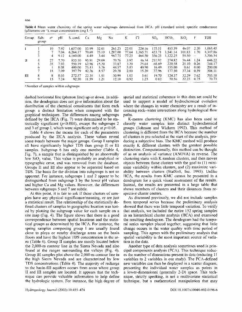
Table 4 Mean water chemistry of the spring water subgroups determined from HCA. pH (standard units); specific conductance ().!Siemens cml), mean concentrations (mg L I)

Group Sub- n" pH S. cond. Ca Mg Na group

1 10 7.92 1,657.00 53.99 32.01 261.23 2 7 7.04 6,264.17 70.69 75.10 1,2R7.00 3 4 9.12 4,160.00 4.40 3.44 967.75

II 4 27 7.70 855.10 95.91 29.09 70.76 5 28 7.92 550.19 62.96 15.20 32.87 6 I 8.08 400.00 25.43 5.76 44.57 7 18 7.09 397.79 42.26 8.57 29.28

111 8 8 8.03 272.57 22.38 1.81 30.99 9 15 7.24 92.50 11.59 1.21 12.10

a Number of samples within subgroups

dashed horizontal line (phenon line) up or down. In addi­tion, the dendogram does not give information about the distribution of the chemical constituents that form each group: a distinct limitation when compared with the graphical techniques. The differences among subgroups defined by the HCA (Fig. 7) were determined to be sta­tistically significant (p<O.OO 1 ), except the subgroups 2 and 3 of group I, which were significant only at p<0.05.

Table 4 shows the means for each of the parameters produced by the HCA analysis. These values reveal some trends between the major groups. Group I samples all have significantly higher TDS than group II or III samples. Subgroup 6 has only one member (Table 4, Fig. 7), a sample that is distinguished by an abnormally low Si02 value. This value is probably an analytical or typographic error, and was removed from the database. Groups II and III also appear to be separated based on TDS. The basis for the division into subgroups is not so apparent. For instance, subgroups 1 and 2 appear to be distinguished from subgroup 3 by the lower pH values and higher Ca and Mg values. However, the differences between subgroups 5 and 7 are subtle.

At this point, it is fair to ask if these clusters of sam­ples have any physical significance/meaning, or are just a statistical result. The relationship of the statistically de­fined clusters of samples to geographic location was test­ed by plotting the subgroup value for each sample on a site map (Fig. 4). The figure shows that there is a good correspondence between spatial locations and the statis­tical groups as determined by the HCA. For instance, the spring samples composing group I are usually found close to playa or nearby discharge areas on the basin floors and have the highest TDS concentration in the ar­ea (Table 4). Group II samples are mostly located below the 2,000-m contour line in the Sierra Nevada and also found at the ranges surrounding the valleys (Fig. 4). Group III samples plot above the 2,000-m contour line in the high Sierra Nevada and are characterized by low TDS concentrations (Table 4). The majority of recharge to the basin-fill aquifers occurs from areas where group II and III samples are located. It appears that the tech­nique can provide valuable information to help define the hydrologic system. For instance, the high degree of

Hydrogeology Journal (2002) 10:455--474

K C1 so4 HC01 Si02 F TDS

22.01 224.16 175.51 453.39 46.07 2.20 1,063.45 77.64 1,165.71 433.71 1,541.14 101.83 1.70 4.347.86 77.25 464.50 336.25 1,122.25 50.50 - 3,206.34

3.92 46.34 211.92 274.82 36.44 1.24 646.22 3.20 25.64 68.69 220.58 25.10 0.26 344.17 5.83 40.90 16.49 155.00 0.61 0.00 200.00 2.80 15.20 37.96 177.50 37.34 0.59 308.11

1.03 5.61 19.70 124.37 32.29 2.62 205.18 0.92 1.23 0.82 70.56 22.23 0.75 70.73

spatial and statistical coherence in this data set could be used to support a model of hydrochemical evolution where the changes in water chemistry are a result of in­creasing rock-water interactions along hydrological flow paths.

K-means clustering (KMC) has also been used to classify water samples into distinct hydrochemical groups (Johnson and Wichern 1992). This method of clustering is different from the HCA because the number of clusters is pre-selected at the start of the analysis, pro­ducing a subjective bias. The KMC method will produce exactly K different clusters with the greatest possible distinction. Computationally, this method can be thought of as an analysis of variance (ANOVA) in reverse. The clustering starts with K random clusters, and then moves objects between those clusters with the goal to (1) mini­mize variability within clusters, and (2) maximize vari­ability between clusters (StatSoft, Inc. 1995). Unlike HCA, the results from KMC cannot be presented in a dendogram for a quick visual assessment of the results. Instead, the results are presented in a large table that shows members of clusters and their distances from re­spective cluster centers.

As discussed previously, we did not include samples from temporal series because the preliminary analysis showed that there was little temporal variation. To verify that analysis, we included the entire 152 spring samples in an hierarchical cluster analysis (HCA) and examined the resulting dendogram. The dendogram had the tempo­ral series samples placed together, suggesting that little change occurs in the water quality with time period of sampling. This agrees with the preliminary analysis that spatial variability is the most important source of varia­tion in the data.

Another type of data analysis sometimes used is prin­cipal components analysis (PCA). This technique reduc­es the number of dimensions present in data (reducing 11 variables to 2 variables in our study). The PCA-defined new variables can then be displayed in a scatter diagram, presenting the individual water samples as points in a lower-dimensional (generally 2-D) space. This tech­nique, strictly speaking, is not a multivariate statistical technique, but a mathematical manipulation that may

DOl 10.1 007/s1 0040-002-0196-6

467

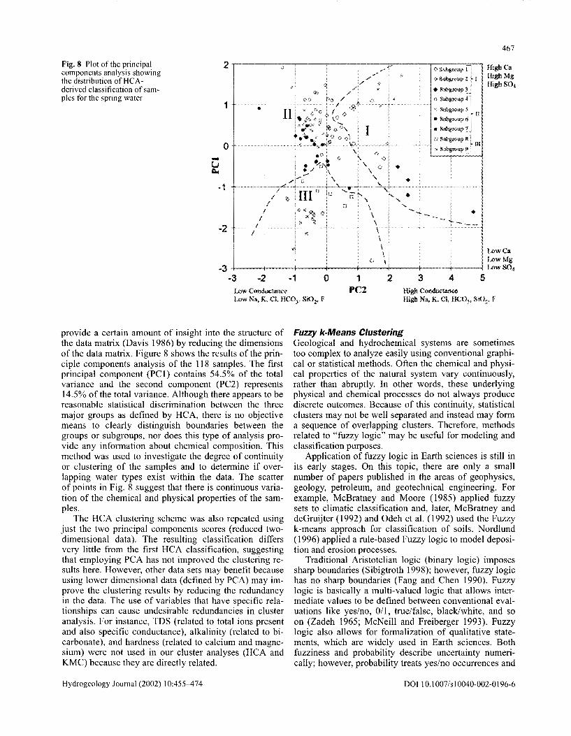
Fig. 8 Plot of the principal components analysis showing the distribution of HC A­derived classification of sam­ples for the spring water

0 Subgroup l I High Mg

2 .,------c-: ~-----:----------.,.,.------,-0-S-~bg-ro-,·u-p-::l~::::----, High Ca

High so4 + SubllJOUp 3

0

<> Subgroup 4>} ' Subg:mup 5 ll

• Su\>gr<>u;p6 .. • Subgro11p 1

o Subgr<>up sl ------~~;;•'7~-~-~¥-''---------------------------··'i--·-·······----·--- ---! • m

Subgn>up 9 :

1 •

I

-u 1:1,.

• -2

l.owCa LowMg

-3 +-----+----1---+---+----+---+---+---·-l I .ow S04 -3 -2 -1 0 1 2 3 4 5

Low Conductance PC2 High Conductance Low Na., K. Cl. HCO;, Si02, F High Na, K. Cl, HC03, Si02• F

provide a certain amount of insight into the structure of the data matrix (Davis 1986) by reducing the dimensions of the data matrix. Figure 8 shows the results of the prin­ciple components analysis of the 118 samples. The first principal component (PC I) contains 54.5% of the total variance and the second component (PC2) represents 14.5% of the total variance. Although there appears to be reasonable statistical discrimination between the three major groups as defined by HCA, there is no objective means to clearly distinguish boundaries between the groups or subgroups, nor does this type of analysis pro­vide any information about chemical composition. This method was used to investigate the degree of continuity or clustering of the samples and to determine if over­lapping water types exist within the data. The scatter of points in Fig. 8 suggest that there is continuous varia­tion of the chemical and physical properties of the sam­ples.

The HCA clustering scheme was also repeated using just the two principal components scores (reduced two­dimensional data). The resulting classification differs very little from the first HCA classification, suggesting that employing PCA has not improved the clustering re­sults here. However, other data sets may benefit because using lower dimensional data (defined by PCA) may im­prove the clustering results by reducing the redundancy in the data. The use of variables that have specific rela­tionships can cause undesirable redundancies in cluster analysis. For instance, TDS (related to total ions present and also specific conductance), alkalinity (related to bi­carbonate), and hardness (related to calcium and magne­sium) were not used in our cluster analyses (HCA and KMC) because they are directly related.

Hydrogeology Journal (2002) I 0:455-4 74

Fuzzy k-Means Clustering Geological and hydrochemical systems are sometimes too complex to analyze easily using conventional graphi­cal or statistical methods. Often the chemical and physi­cal properties of the natural system vary continuously, rather than abruptly. In other words, these underlying physical and chemical processes do not always produce discrete outcomes. Because of this continuity, statistical clusters may not be well separated and instead may form a sequence of overlapping clusters. Therefore, methods related to "fuzzy logic" may be useful for modeling and classification purposes.

Application of fuzzy logic in Earth sciences is still in its early stages. On this topic, there are only a small number of papers published in the areas of geophysics, geology, petroleum, and geotechnical engineering. For example, McBratney and Moore (1985) applied fuzzy sets to climatic classification and, later, McBratney and deGruijter (1992) and Odeh et al. (1992) used the Fuzzy k-means approach for classification of soils. Nordlund ( 1996) applied a rule-based Fuzzy logic to model deposi­tion and erosion processes.

Traditional Aristotelian logic (binary logic) imposes sharp boundaries (Sibigtroth 1998); however, fuzzy logic has no sharp boundaries (Fang and Chen 1990). Fuzzy logic is basically a multi-valued logic that allows inter­mediate values to be defined between conventional eval­uations like yes/no, 0/1, true/false, black/white, and so on (Zadeh 1965; McNeill and Freiberger 1993). Fuzzy logic also allows for formalization of qualitative state­ments, which are widely used in Earth sciences. Both fuzziness and probability describe uncertainty numeri­cally; however, probability treats yes/no occurrences and

DOl I 0.1 007/sl 0040-002-0196-6

468

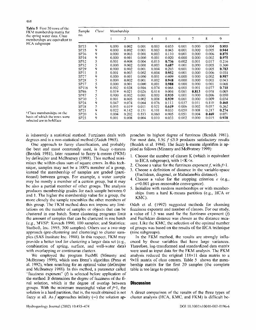
Table 5 First 20 rows of the FKM membership matrix for Sample Class" Membership the spring water data. Class no. memberships are equivalent to 2 3 4 5 6 7 8 9 HCA subgroups

SP33 9 0.000 0.002 0.001 0.003 0.033 0.001 0.000 0.004 0.955 SP35 9 0.000 0.002 0.001 0.003 0.043 0.001 0.000 0.005 0.944 SP36 9 0.000 0.003 0.001 0.003 0.110 0.001 0.000 0.006 0.875 SP34 9 0.000 0.001 0.000 0.001 0.020 0.000 0.000 0.002 0.975 SP52 5 0.001 0.008 0.004 0.015 0.736 0.002 0.001 0.017 0.216 SP32 5 0.000 0.002 0.001 0.003 0.687 0.001 0.000 0.005 0.300 SP29 9 0.000 0.002 0.001 0.004 0.203 0.001 0.000 0.005 0.783 SP31 5 0.001 0.003 0.002 0.004 0.952 0.001 0.000 0.006 0.031 SP27 9 0.000 0.001 0.000 0.001 0.009 0.000 0.000 0.002 0.987 SP28 5 0.000 0.002 0.001 0.002 0.948 0.000 0.000 0.003 0.043 SP37 5 0.000 0.001 0.000 0.001 0.988 0.000 0.000 0.001 0.008 SP116 9 0.002 0.038 0.016 0.074 0.068 0.005 0.001 0.077 0.718 SP86 7 0.019 0.021 0.026 0.014 0.004 0.081 0.813 0.018 0.005 SP47 5 0.000 0.002 0.001 0.003 0.935 0.001 0.000 0.006 0.050 SP30 5 0.001 0.005 0.002 0.008 0.939 0.001 0.000 0.009 0.034 SP24 9 0.047 0.074 0.064 0.076 0.113 0.037 0.011 0.110 0.468 SP38 5 0.003 0.019 0.011 0.021 0.619 0.006 0.002 0.057 0.262 SP21 9 0.022 0.142 0.151 0.101 0.033 0.050 0.008 0.217 0.274

a Class memberships on the SP20 8 0.004 0.202 0.183 basis of which the rows were

0.060 0.005 0.051 0.004 0.469 0.021 SP25 9 0.001 0.008 0.004 0.010 0.033 0.002 0.000 0.015 0.928

selected are in boldface

is inherently a statistical method. Fuzziness deals with degrees and is a non-statistical method (Zadeh I 965).

One approach to fuzzy classification, and probably the best and most commonly used, is fuzzy c-means (Bezdek 1981), later renamed to fuzzy k-means (FKM) by deGruijter and McBratney (1988). This method mini­mizes the within-class sum of square errors. In this tech­nique, samples may not be a 100% member of a group, instead the membership of samples are graded (parti­tioned) between groups. For example, a water sample may be mostly a member of a certain group, but it may be also a partial member of other groups. The analysis produces membership grades for each sample between 0 and 1. The higher the membership value for a group, the more closely the sample resembles the other members of this group. The FKM method does not impose any limi­tations on the number of samples or objects that can be clustered in one batch. Some clustering programs limit the amount of samples that can be clustered in one batch (e.g., MVSP: Kovach 1990, 100 samples; and Statistica: StatSoft, Inc. 1995, 300 samples). Others use a two-step approach (pre-clustering and clustering) to cluster sam­ples (SAS Institute Inc. 1988). In this respect, FKM may provide a better tool for clustering a larger data set (e.g., combination of spring, surface, and well-water data) with overlapping or continuous clusters.

We employed the program FuzME (Minasny and McBratney 1999), which uses Brent's algorithm (Press et al. I 992), when searching for an optimal value ( deGruijter and McBratney 1988). In this method, a parameter called "fuzziness exponent" (j) is selected before application of the method. It determines the degree of fuzziness of the fi­nal solution, which is the degree of overlap between groups. With the minimum meaningful value off= 1, the solution is a hard partition, that is, the result obtained is not fuzzy at all. As f approaches infinity ( oo) the solution ap-

Hydrogeology Journal (2002) 10:455-474

proaches its highest degree of fuzziness (Bezdek 1981 ). For most data, 1.5:::; f ::;3.0 produces satisfactory results (Bezdek et al. 1984). The fuzzy k-means algorithm is ap­plied as follows (Minasny and McBratney 1999):

1. Choose the number of classes K (which is equivalent to HCA subgroups), with 1<K<n.

2. Choose a value for the fuzziness exponent f, with f> 1. 3. Choose a definition of distance in the variable-space

(Euclidean, diagonal, or Mahalanobis distance). 4. Choose a value for the stopping criterion e (e.g.,

e=0.001 gives reasonable convergence). 5. Initialize with random memberships or with member­

ships from a hard K-means partition (e.g., HCA or KMC).

Odeh et al. (1992) suggested methods for choosing fuzziness exponent and number of classes. For our study, a value of 1.5 was used for the fuzziness exponent (j) and Euclidean distance was chosen as the distance mea­sure. Like the KMC, the selection of the optimal number of groups was based on the results of the HCA technique (nine subgroups).

In the FKM method, the results are strongly influ­enced by those variables that have large variances. Therefore, log-transformed and standardized data matrix were used as input data for the FKM analysis. The FKM analysis reduced the original 118xll data matrix to a 9xll matrix of class centers. Table 5 shows the mem­bership matrix for the first 20 samples (the complete table is too large to present).

Discussion

A direct comparison of the results of the three types of cluster analysis (HCA, KMC, and FKM) is difficult be-

DOl 10.1 007 /s I 0040-002-0196-6

Fig. 9 Piper diagram of the nine subgroup means for the clusters defined by the three ditlcrent methods

PIPER DIAGRAM

469

() Fuzzy k-means Clustering 6 Hierarchical Cluster Analysis [] K-means Clustering

Numbers in parenthesis show the number of samples in that particular subgroup,

cause only the HCA technique produces a graphical out­put. Therefore, we plotted the HCA-, KMC- and FKM­defined means for each subgroup on a Piper diagram. Figure 9 shows that the HCA-, KMC- and FKM-defined means for each group overlap for most of the subgroups, showing the similar results obtained for all three methods. For instance, the FKM analysis placed 97% of the samples within the same three major groups defined by HCA method, whereas 79% of the samples are placed exactly into same subgroups. However, in both the KMC and FKM analysis, we had pre-selected the number of groups (in our case that number was based on the nine defined by the HCA results). The similarity of the results for all three techniques suggests that the pre-selection of the number of groups strongly influences the outcome. This is a serious limitation that means the investigator is required to have performed some type of preliminary analysis when employing the KMC and FKM tech­niques, which could then bias the results of the statistical analysis.

The efficiency and semi-objective nature of the statis­tical techniques makes these techniques superior to the graphical methods in order to group samples based on water chemistry data. However, the graphical methods

Hydrogeology Journal (2002) I 0:455--4 74

provide valuable information about the chemical nature of the groups. By combining the two techniques we can gain additional information that neither technique by it­self can offer.

Figure I Oa-c shows the mean values for each of the nine subgroups (defined by HCA) on Collins bar, pie, and Stiff diagrams, respectively. Each graphical tech­nique shows distinct visual differences between the sub­groups, while providing information about the chemical composition of each group. In Fig. II, all the samples are plotted on Schoeller semi-logarithmic diagrams for each subgroup. This plot illustrates the difficulty in using purely graphical means to cluster samples. The patterns of subgroups I and 2 are distinctive, but subgroup 3 does not appear related. However, although subgroups 4-7 show a distinct pattern that differs from the other sub­groups, it would be difficult to discriminate between samples belonging to subgroups 4-7.

Although previously not utilized in the classification of water samples, we have included an example of icon plots that can be used to represent and visually discern similarities between water samples. The basic idea of icon plots is to represent individual water samples as graphical objects where values of variables are assigned

DOl I 0.1 007/sl 0040-002-0196-6

470

Fig. 10 Plots of a Collins bar diagram, b pie diagram, and c Stiff pattern using subgroup means defined by HC A

Cullin!! Bar l>iagtllm

I Sl1\w<11p I $~ 2 ~ 3 !l Subgrouf> 4 S~ 5 l>'ubgroop 6 Suhgnmp 7 I I Snhgtoop 8 Subgroup 91

Group 1 Group 11 Group III

Pic Diagram 1:.Jpper HalfofCirdc Lower llalf of eircle

Subgroup 4

to specific features or dimensions of the objects. The as­signment is such that the overall appearance of the ob­jects changes as a function of the configuration of val­ues. Thus, the objects are given visual "identities'' that are unique for configurations of values. One of the most

Hydrogeology Journal (2002) I 0:455-474

Subgroup 5 Subgroup 6

Group II

Stift'Pattem

Subgroup 8 I t Group Ill

Subgroup 9

t

Subgroup 7

Group I

n-.ecy'L Alill:!l!llL....

Subgroup4 -Subgroup 5

~ Group Subgroup 6 TI

t Subgroup 7

t elaborate type of icon plot is Chernoff faces (Chernoff 1973 ), which can be used to plot up to 20 parameters for one water sample. Chernoff faces were plotted for the subgroup means from the cluster analysis (Fig. 12). This technique also provides an effective visualization of a

DOl I 0.1 007/sl 0040-002-0196-6

Subgroup l

10

~ O.f

Subgroup4

!()()

1 n 1

I).GI

0 001

SubgroupS HKl~

IU: l l · · ...ll~l ----

<Jo $ 0 J --

' I I {}{}] J l

OMt•· J ........ I · ·' Ca \1g t\• K

Subgroup 8 !00 , .............. , ........... .

471

>lubgroup 3

100

10

~ G D.l

Group nj 0.01

I .............. ········•

C! SG4 KCO, Mg Na K

Suhgmup9

Fig. 11 Plots of all spring water samples by using Schoeller diagram (subgroups and groups defined by HC A)

Fig. 12 Chernotf faces (sub­groups and groups defined by 1-!CA)

Hydrogeology Journal (2002) 10:455--474

kon Plot (Ciu~ruoff Fat-es) I \Pj.,\\'.\J'I(>N

Width .. ,fh~e·e Ca

l~.:cmn.:·•t\· nt'uppcr !ilc·c \lg,

L<X~tlll11.1h <>fltll\c'J' fi"" \';I ! .<:nglh <)f ll••~c K \\ tchh •'I' '\1>•.~ C1 Cun ;Utuv ,fmot>lh S( )4

! '-'llt:lh ••fmnmh I!C<l1

i la)f.fac~ h(•tgln SiOc

S.;p;mt1!0f1 ,,f ~\~' !' i <:liglft of ri\chm\'> ·· pi! R;"hus. t>l ~ar C<>ndu..:t:.mw

DO I I 0.1 007 /s I 0040-002-0196-6

472

small number of water samples having different charac­teristics. The different physical and chemical characteris­tics of the samples are shown by the changes in facial features. Parameter values are represented in schematic humanlike faces such that the values for each variable are represented by the variations of specific facial fea­tures (StatSoft, Inc. I 995). Examining such plots may help to discover specific clusters of both simple relations and interactions between variables.

Summary and Conclusions

Each technique that has been discussed in this paper has advantages and disadvantages in clustering and display­ing water samples using typical chemical and physical parameters. The graphical techniques can provide valu­able and rapidly accessible information about the chemi­cal composition of water samples such as the relative proportion of the major ions; however, these techniques have some serious limitations when used alone. All the graphical techniques use only a portion of the available data. Minor constituents (0.01-10 mg L-1; e.g., boron, fluoride, iron, nitrate, strontium) and trace constituents (<0.1 mg L-1; e.g., aluminum, arsenic, barium, bromide, chromium, lead, lithium) are not used. From a water­quality standpoint, the presence of one of these minor or trace elements may be important because small amounts can pose threats to human health. Some of these minor and trace constituents behave more conservatively in the groundwater, thus, they can be used more efficiently to classify waters (Farnham et a!. 2000). Some graphical techniques can display only one sample (or a mean) per diagram (e.g., Collins bar, pie, Stiff), whereas others can display multiple samples (e.g., Piper, Schoeller). Neither type is particularly useful to produce distinct grouping of samples because there is no objective means to discrimi­nate the groups or to test the degree of similarity be­tween samples in a group. Collins bar, pie, and Stiff dia­grams are probably the best to help distinguish between small numbers of samples that have distinct chemical differences. For a large number of samples these dia­grams are unwieldy. In this study, neither the Piper nor Schoeller diagrams could group all the similar water sam­ples (based on statistical measures) from our data set.

Unlike the graphical classification techniques, multivar­iate statistical techniques can use any combination of chemical and physical parameters (e.g., temperature) to classify water samples. The HCA technique was judged more efficient than the KMC and FKM techniques because it offers a semi-objective graphical clustering procedure (dendogram), which does not require pre-determining the final number of clusters. However, none of the statistical techniques offered easily accessible information about the chemical composition of the samples in the clusters (groups). That is, these methods are very efficient at group­ing water sample by physical and chemical similarities, but the results are not immediately useful for identifying trends or processes relevant to hydrogeochemical problems.

Hydrogeology Journal (2002) I 0:455-4 74

Combining the two approaches appears to offer a methodology that retains the advantages while minimiz­ing the limitations of either approach. Using the HCA analysis to initially cluster the samples (into groups and subgroups) provides an efficient means to recognize groups of samples that have similar chemical and physi­cal characteristics. The technique also allows discrimina­tion of samples that have extreme values for closer eval­uation. These statistical groups have distinct spatial pat­terns in the study area, providing the spatial discrimina­tion desired when determining hydrochemical facies. The mean for each of the required chemical parameters are then plotted on diagrams, e.g., a Piper diagram, offer­ing easily accessible information on the chemical differ­ences between the groups and potential information about the physical and chemical processes in the water­shed. The use of the hierarchical cluster analysis (HCA) in conjunction with a multi-sample graphical technique such as the Piper plot offers a robust methodology with consistent and objective criteria to efficiently classify large numbers of water samples based on common chemical and physical parameters.

Acknowledgements The authors would like to thank reviewers, Dr. Patrice deCaritat and Dr. K.H. Johannesson. for their thorough critique. This study was fully sponsored by the Ministry of Na­tional Education ofTurkey.

References

Alther GA (1979) A simplified statistical sequence applied to rou­tine water quality analysis: a case history. Ground Water 17:556-561

Back W (1961) Techniques for mapping of hydrochemical facies. US Geol Surv Prof Pap 424-D, pp 380-382

Back W ( 1966) Hydrochemical facies and groundwater flow pat­terns in northern part of Atlantic Coastal Plain. US Geol Surv Prof Pap 498-A. Washington, DC

Back W, Hanshaw BB ( 1965) Chemical geohydrology. Adv Hydrosci 2:49-109

Barnes I, Kistler RW, Mariner RH, Presser TS ( 1981) Geochemi­cal evidence on the nature of the basement rocks of the Sierra Nevada, California. US Geol Surv Water-Supply Pap 2181, 13 pp

Berenbrock C ( 1987) Ground-water data for Indian Wells Valley, Kern, lnyo, and San Bernardino Counties, California, 1977-84. US Geol Surv Open-File Rep 86-315, 56 pp

Berenbrock C, Schroeder RA (1994) Ground-water flow and qual­ity, and geochemical processes, in Indian Wells Valley, Kern, lnyo and San Bernardino Counties, California, 1987-88. US Geol Surv Water-Resour Invest Rep 93-4003, 59 pp

Berry JK (1995) Spatial reasoning for ctfective GIS. GIS World Books, Fort Collins, Colorado

Bezdek JC ( 198 I) Pattern recognition with fuzzy objective func­tion algorithms. Plenum Press, New York

Bezdek JC, Ehrlich R, Full W (1984) FCM: the fuzzy c-means clustering algorithm. Comput Geosci 10:191-203

Brown E. Skougstad MW. Fishman MJ ( 1970) Methods for collec­tion and analysis of water samples for dissolved minerals and gases. US Geol Surv Tech Water-Resour Invest, TWI 5-A I, 160 pp

Buono A, Packard EM (1982) Evaluation of increases in dissolved solids in ground water, Stovepipe Wells Hotel, Death Valley National Monument, California. US Gcol Surv Open-File Rep 82-513,23pp

DOl I 0.1 007/s I 0040-002-0196-6

Chernoff H ( 1973) The use of faces to represent points in k-dimensional space graphically. JAm Stat Assoc 68:361-368

Collins WD ( 1923) Graphic representation of water analyses. lnd Eng Chem 15:394

Davis JC ( 1986) Statistics and data analysis in geology, 2nd edn. Wiley, New York

deGruijter JJ, McBratney AB ( 1988) A modified Fuzzy k-mcans for predictive classification. In: Bock HH (ed) Classification and related methods of data analysis. Elsevier Science, Amsterdam

Dockter RD ( I980a) Geophysical, lithologic and water-quality da­ta from test well CU-2, Cuddeback dry lake, San Bernardino County, California. US Geol Surv Open-File Rep 80-1033. I sheet

Dockter RD ( !980b) Geophysical, lithologic, and water-quality data from test well CU-I, Cuddeback dry lake, San Bernardino County, California. US Geol Surv Open-File Rep 80-1034, I sheet

Domenico PA, Schwartz FW ( 1997) Physical and chemical hydro­geology, 2nd edn. Wiley, New York

Drcvcr Jl (I 997) The geochemistry of natural waters, 3rd edn. Prentice-Hall, Upper Saddle River, NJ

Duffield WA, Smith GI (1978) Pleistocene history of volcanism and the Owens River near Little Lake, California. J Res US Geol Surv 6:395-408

Dutcher LC, Moyle WR Jr (1973) Geologic and hydrologic fea­tures of Indian Wells Valley, California. US Geol Surv Water­Supply Pap 2007, 30 pp

Fang JH, Chen HC (I 990) Uncertainties are better handled by Fuzzy arithmetic. Am Assoc Petrol Geol Bull 74: 1128-1233

Farnham IM, Stetzenbach KJ, Singh AK, Johannesson KH (2000) Deciphering groundwater flow systems in Oasis Valley, Neva­da, using trace element geochemistry, multivariate statistics, and geographical information system. Math Geol 32:943-968

Farnham IM, Stetzenbach KJ, Singh AS, Johanncsson KH (2002) Treatment of nondetects in multivariate analysis of ground­water geochemistry data. Chemometrics Intelligent Lab Sys 60:265-281

Fenneman NM ( 1931) Physiography of western United States. McGraw-Hill Book Company. New York

Feth JH, Roberson CE, Polzer WL (1964) Sources of mineral con­stituents in water from granitic rocks, Sierra Nevada, Califor­nia and Nevada. US Geol Surv Water-Supply Pap 1535-1, p 11-170

Font KR (I 995) Geochemical and isotopic evidence for hydrologic processes at Owens Lake, California. MSc Thesis University of Nevada, Reno, 219 pp

Fournier RO. Thompson JM ( 1980) The recharge area for the Coso, California, geothermal system deduced from liD and 8180 in thermal and non-thermal waters in the region. US Geol Surv Open-File Rep 80-454, 24 pp

Freeze RA, Cherry JA ( 1979) Groundwater. Prentice Hall, Engle­wood Cliffs, NJ

Hem JD ( 1989) Study and interpretation of the chemical charac­teristics of natural water, 3rd edn. US Geol Surv Water-Supply Pap 2254, 263 pp

Hill RA ( 1940) Geochemical patterns in Coachella Valley. Trans Am Geophys Union 2 I :46-49

Hill RA ( 1942) Salts in irrigation waters. Trans Am Soc Civil Eng 107:1478-1493

Hollett KJ, Danskin WR, McCaffrey WF, Walti CL ( 1991) Geolo­gy and water resources of Owens Valley, California. US Geol Surv Water-Supply Pap 2370-B, 77 pp

Houghton BD (1994) Ground water geochemistry of the Indian Wells Valley. MSc Thesis, California State University, Bakers­field, 85 pp

Hunt CB, Robinson TW, Bowles WA, Washburn AL (1966) Hy­drologic basin, Death Valley, California. US Gcol Surv Prof Pap 494-B, 138 pp

Jaquet JM, Froidevoux R, Verncd JP ( 1975) Comparison of auto­matic classification methods applied to lake geochemical sam­ples. Math Geol 7:237-265

Hydrogeology Journal (2002) I 0:455-4 74

473

Johnson JA ( 1993) Water resources data California water year 1993, vol 5, ground-water data. US Geol Surv Water-Data Rep CA-93-5, pp 97-270

Johnson JA, Fong-Frydendal LJ, Baker JB ( 1991) Water resources data California water year I 991, vol 5, ground-water data. US Gcol Surv Water-Data Rep CA-9 I -5, pp 6 I -62

Johnson RA, Wichern DW ( 1992) Applied multivariate statistical analysis. Prentice Hall, Englewood Cliffs, NJ

Judd AG ( 1980) The use of cluster analysis in the derivation of geotechnical classifications. Bull Assoc Eng Geol 17:193-21 I

Kovach WL ( 1990) A multivariate statistical package. Institute of Earth Studies, University College of Wales, Aberystwyth, Wales SY23 3DB, UK

Lamb CE, Keeter GL, Grillo DA (1986) Water resources data California water year 1986, vol 5, ground-water data for California. US Geol Surv Water-Data Rep CA-86-5, pp 34-185

Lee CH ( 1912) Ground water resources of Indian Wells Valley, California. California State Conservation Commission Report, pp 403-429

Lipinski P, Knochenmus DD (1981) A I 0-Year plan to study the aquifer system of Indian Wells Valley, California. US Geol Surv Open-File Rep 81-404, 18 pp

Lopes TJ (1987) Hydrology and water budget of Owens Lake, California. MSc Thesis, University of Nevada, Reno, 127 pp

Maltby DE, Downing KT, Keeter GL, Lamb CE ( 1985) Water re­sources data California water year 1985, vol 5, ground-water data for California. US Geol Surv Water-Data Rep CA-85-5, pp 42-207

Maxey GB ( 1968) Hydrogeology of desert basins. Ground Water 6:10--22

McBratney AB, deGruijter JJ ( 1992) A continuum approach to soil classification by modified Fuzzy k-mcans with extra­grades. J Soil Sci 43:159-175

McBratney AB, Moore A W ( 1985) Application of fuzzy sets to climatic classification. Agric For Meteorol 35: I 65-185

McHugh JB, Ficklin WH. Miller WR ( 198 I) Analytical results of 78 water samples from Domeland Wilderness and adjacent further planning areas (RARE II), California. US Geol Surv Open-File Rep 81-730, 17 pp

McNeill D, Freiberger P (1993) Fuzzy logic - the revolutionary computer technology that is changing our world. Simon and Schuster, New York

Melack JM, Stoddard JL, Ochs CA (1985) Major ion chemistry and sensitivity to acid precipitation of Sierra Nevada lakes. Water Resour Res 21:27-32

Microsoft Corporation ( 1985) Microsoft Excel 97 spreadsheet software

Miesch AT ( 1976) Geochemical survey of Missouri -methods of sampling, laboratory analysis and statistical reduction of data. US Geol Surv Prof Pap 954-A, 39 pp

Miller GA ( 1977) Appraisal of the water resources of Death Valley, California-Nevada. US Geol Surv Open-File Rep 77-728. 68 pp

Minasny B, McBratney AB ( 1999) FuzME (Fuzzy k-Means with Extragrades) version 1.0. Australian Centre for Precision Agriculture, McMillan Building A05, University of Sydney. http://www.usyd.edu.au/su/agric/acpa

Moyle WR Jr (1963) Data on water wells in Indian Wells Valley area, lnyo, Kern, and San Bernardino Counties, California. California Dept Water Resour Bull 9 I -9, 243 pp

Moyle WR Jr ( 1969) Water wells and springs in Panamint, Searles, and Knob Valleys, San Bernardino and lnyo Coun­ties, California. California Dept Water Resour Bull 91-17, I 10 p

Moyle WR Jr (1971) Water wells in the Harper, Superior, and Cuddeback Valley areas, San Bernardino County, California. California Dept of Water Resour Bull 91-19, 99 pp

Nordlund U (1996) Formalizing geological knowledge- with an example of modeling stratigraphy using Fuzzy logic. J Sedi­ment Res 66:689-698

DOT I 0.1 007/sl 0040-002-0196-6

474

Odeh lOA, McBratney AB, Chittleborough DJ ( 1992) Soil pattern recognition with Fuzzy c-means: application to classification and soil-landform interrelationships. Soil Sci Soc Am J 56:505-516

Ostdick JR ( 1997) The hydrogeology of southwest Indian Wells Valley, Kern County, California: evidence for extrabasinal, fracture-directed groundwater recharge from the adjacent Sierra Nevada Mountains. MSc Thesis, California State Uni­versity, Bakersfield, 128 pp

Piper AM (1944) A graphic procedure in the geochemical inter­pretation of water-analyses. Trans Am Geophys Union 25: 914-923

Press WH, Teukolsky SA, Vetter ling WT, Flannery BP ( 1992) Nu­merical recipes: the art of scientific computing. Cambridge University Press, Cambridge. http://www.nr.com

Robinson BP, Beetem WA (1975) Quality of water in aquifers of the Amargosa Desert and vicinity, Nevada. US Geol Surv Rep 474-215,64pp

Rock Ware, Inc. ( 1999) Rock Works plotting software. Golden, Colorado

Rummel RJ ( 1970) Applied factor analysis. Northwestern Univer­sity Press, Evanston

Sanford RF, Pierson CT. Crovelli RA ( 1993) An objective replace­ment method for censored geochemical data. Math Geol 25:59-80

SAS Institute, Inc. ( 1988) SAS/STAT user's guide, release 6.03 edn. SAS Institute Inc. Cary, NC, I 028 pp

Schoeller H ( 1955) Geochemie des eaux souterraines. Rev Inst Fr Petrol I 0:230-244

Hydrogeology Journal (2002) 10:455--474

Schoeller H ( 1962) Les eaux souterraines. Massio et Cie, Paris, France

Sibigtroth J ( 1998) A graphical introduction to fuzzy logic. http://www.mcu.motsps.com/lit/tutor/fuzzy/fuzzy.html

StatSoft, Inc. ( 1995) STATISTICA for Windows (computer pro­gram manual), vol 3. StatSoft, Inc. Tulsa, OK

StatSoft, Inc. ( 1997) Electronic statistics textbook. StatSoft, Inc. Tulsa, OK. http://www.statsoft.com/textbook/stathome.html

Stiff HA Jr ( 1951) The interpretation of chemical water analysis by means of patterns. J Petrol Tech 3:15-17

US Bureau of Reclamation ( 1993) Indian Wells Valley ground­water project. US Bureau of Reclamation Technical Report, vols 1-11

Van Trump G Jr, Miesch AT ( 1977) The US Geological Survey RASS-STATPAC system for management and statistical re­duction of geochemical data. Com put Geosci 3:475--488

Ward JH (1963) Hierarchical grouping to optimize an objective function. J Am Stat Assoc 69:236-244

Whelan JA, Baskin R, Katzenstein AM (1989) A water geochem­istry study of Indian Wells Valley, Inyo and Kern Counties, California, vol I, geochemistry study and appendix A. Naval Weapons Center Technical Publication 7019,54 pp

Williams RE ( 1982) Statistical identification of hydraulic connec­tions between the surface of a mountain and internal mineral­ized zones. Ground Water 20:466-4 78

Wood WW ( 1981) Guidelines for collection and tield analysis of ground-water samples for selected unstable constituents. Tech Water-Resour Invest US Geol Surv, 24 pp

Zadeh LA ( 1965) Fuzzy sets. Infonn Control 8:338-353

DOl I 0.1 007/sl 0040-002-0196-6