Essays on Economic and Econometric Modelling
of Behavioral Heterogeneity in Demand Theory
Ralf Wilke

Universitat Dortmund
Fachbereich fur Wirtschafts- und Sozialwissenschaften
DFG Graduiertenkolleg
Allokationstheorie, Wirtschaftspolitik und kollektive Entscheidungen
Dissertation
Essays on Economic and Econometric
Modelling of Behavioral Heterogeneity in
Demand Theory
Ralf Andreas Wilke
Dortmund, 4.2002

Vorwort
Die Modellierung des individuellen Verhaltens der Subjekte einer Okonomie ist in der
Regel das Fundament der Wirtschaftstheorie, auf dem Aussagen abgeleitet werden.
Der entsprechende Modellierungsansatz wird durch Vermutungen an jenes Verhal-
ten begrundet. Ergebnisse sind daher meistens das Resultat von Annahmen. Sie
sind demnach nicht allgemein gultig, sondern halten nur in dem vorgegebenen Mo-
dellrahmen. Es ist in der Regel leicht zu zeigen, dass diese Ergebnisse nicht erzielt
werden, wenn entsprechende Bedingungen verletzt sind. Ausserdem ist es meistens
nicht schwierig zu sehen, dass Vermutungen uber individuelles Verhalten in der Rea-
litat bestenfalls fur eine Gruppe von Individuen oder Wirtschaftssubjekten erfullt
sind, jedoch fast sicher nicht fur alle Individuen einer Population. Damit stellt sich
die Frage, auf welche Berechtigung sich die Wirtschaftstheorie stutzt, diese Vorge-
hensweise weiterzufuhren.
Es soll und kann nicht das Ziel der vorliegenden Dissertation sein, eine Antwort
auf diese Fragestellung zu liefern. Vielmehr sollte sie jeder Wissenschaftler selbst be-
antworten, seine Ziele definieren und entsprechende Methoden wahlen oder erfinden,
um diese zu erreichen. Deshalb sollte ein Wissenschaftler in zumindest den folgenden
drei Kriterien uber gewisse Fahigkeiten verfugen: Kritik, Innovation, Technik.
Diese Dissertation liefert vielmehr einige Beitrage zu einer interessanten Vorge-
hensweise, das angedeutete Dilemma der Wirtschaftstheorie zumindest in Teilen zu
uberwinden. Die zugrundeliegende Idee ist dabei nicht, das Verhalten jedes Indivi-
duums zu spezifizieren, sondern vielmehr die Bevolkerung als Ganzes zu betrachten
und aufgrund von einer gewissen Heterogenitat in der Bevolkerung Gesetzmassig-
keiten fur das durchschnittliche Verhalten abzuleiten. Bei der Modellierung spielen
z.B. die Verteilung des verfugbaren Einkommens von Haushalten oder Unterschiede
im Verhalten eine wichtige Rolle. Die Dissertation liefert Beitrage zur Methodik der
Wirtschaftstheorie und der Okonometrie, die einen Schritt ermoglicht hin zu ange-
wandteren Problemstellungen. Der Rahmen dieser Beitrage ist die Nachfragetheorie.
Er wurde gewahlt, da es in diesem Bereich bereits eine Reihe von Forschungen gibt,
die diese Art der Modellierung eingefuhrt und bearbeitet haben. Das Gebiet ist
daruber hinaus interessant, da es hinreichend grosse Datensatze gibt, die komplexe
okonometrische Untersuchungen erlauben.
2

Diese Arbeit gliedert sich in zwei Teile. Der erste Teil umfasst drei Beitrage zur
Wirtschaftstheorie. Der erste Beitrag fasst bestehende Ergebnisse der Nachfrage-
theorie zusammen. Dieser Uberblick erstreckt sich von klassischen, auf Nutzenmaxi-
mierungsprinzipien beruhenden Ansatzen bis hin zu den neueren verteilungstheore-
tischen Ansatzen. Der zweite Beitrag untersucht, wie die Aggregation von beliebigen
Bevolkerungen strukturelle Eigenschaften der aggregierten Nachfrage erzeugen kann.
Dabei stellt sich in dem gewahlten Rahmen heraus, dass durch die Aufteilung der
Bevolkerung in homogene Teilbevolkerungen strukturelle Eigenschaften der aggre-
gierten Nachfrage verloren gehen konnen. Im dritten Beitrag zur Wirtschaftstheorie
werden in einem allgemeinen Modellrahmen einige Eigenschaften fur die Verteilung
von individuellem Verhalten und des Einkommens von Haushalten hergeleitet, so-
dass die durchschnittliche Nachfrage das Law of Demand erfullt. Ausserdem werden
die in der Literatur eingefuhrten Konzepte und Definition von Verhaltensheteroge-
nitat verglichen und es wird untersucht, welche Arten von Verhaltensheterogenitat
wie zu interpretieren sind. Ein neues Konzept der Verhaltensunterschiede wird ein-
gefuhrt und so definiert, dass es messbar ist.
Der zweite Teil der Arbeit beschaftigt sich in zwei Beitragen mit der okono-
metrischen Modellierung von Verhaltensheterogenitat. Es sollen Nachfragesysteme
modelliert werden, die auf der einen Seite genugend Flexibilitat besitzen, ein breites
Spektrum an individuellem Verhalten zuzulassen, aber auf der anderen Seite nicht
zu grosse Datensatze benotigen, um konkrete und prazise Aussagen zu treffen. Die-
ser Trade-Off wird mit Hilfe von semiparametrischen Schatzern durchbrochen, deren
nichtparametrischer Teil genugend Flexibilitat und deren parametrischer Teil eine
hohe Konvergenzrate bietet. Im ersten Beitrag dieses Teils werden zwei Schatzer
fur Ausgabenanteilsfunktionen und Engel-Kurven vorgeschlagen, die nicht das kon-
krete Verhalten von Haushalten, sondern nur systematische Unterschiede zwischen
homogenen Gruppen von Haushalten parametrisieren. Simulationen untersuchen die
Leistungsfahigkeit dieser Schatzer in endlichen Stichproben unter richtigen Spezifika-
tionen und unter Fehlspezifikationen. Im zweiten Beitrag wird ein weiterer Schatzer
fur die Schatzung von Engel-Kurven eingefuhrt, der mit bereits in der Literatur exi-
stierenden Schatzern vergleichbar ist. Simulationen bescheinigen dem neuen Schatzer
eine uberlegene Leistungsfahigkeit im Vergleich zu den existierenden Ansatzen. Die
Bedingungen fur die Konsistenz des Schatzer werden hergeleitet. Daruber hinaus
3

wird der Schatzer auf Konsumdaten angewendet. Die Ergebnisse zeigen die Rele-
vanz dieser Methode fur die angewandte Mikrookonometrie.
Diese Arbeit wurde im Rahmen des DFG Graduiertenkollegs Allokationstheorie,
Wirtschaftspolitik und kollektive Entscheidungen an den Universitaten Dortmund
und Bochum erstellt. Ein Teil der Beitrage wurde in den Workshops des Gradu-
iertenkolleges an der Universitat Dortmund, dem Workshop uber Okonomien mit
heterogenen Agenten an der Universiteit Maastricht und dem Okonometrie Seminar
an der University of Pittsburgh vorgestellt. Ich bedanke mich bei allen Teilnehmern
fur ihre Kommentare. Insbesondere danke ich Marina Bauer, Dinko Dimitrov, Luis
Gonzalez, Christian Kleiber, Walter Kramer, Wolfgang Leininger und Thomas Spar-
la fur detaillierte Hinweise und Diskussionen. Ein Teil der Arbeit wurde im Rahmen
eines Marie Curie Training Research Fellowships am University College London, De-
partment of Economics, durchgefuhrt. Ich bedanke mich bei den Teilnehmern des
Metrics Lunch Seminars und des Student Lunch Seminars fur Ihre Kommentare.
Besonderer Dank gilt hier Richard Blundell und Hidehiko Ichimura fur die Betreu-
ung eines Teiles der Arbeit und letzterem ausserdem fur das intensive Training in
Asymptotik. Ausserdem bedanke ich mich bei Ben Groom und Katrin Voss fur die
sprachliche Korrektur meiner Arbeit.
4
Inhaltsverzeichnis
I Economic Modelling 6
1 A Selective Survey of Demand Theory 6
2 A Note of Behavioral Heterogeneity and Aggregation 23
3 Behavioral Heterogeneity and the Law of Demand 38
II Econometric Modelling 69
4 Semiparametric Estimation of Consumer Demand 69
5 Semiparametric Estimation of Regression Functions under Shape
Invariance Restrictions 100
5

Essay 1
A Selective Survey of Demand Theory
April 22, 2002
Abstract
This essay surveys recent approaches to the explanation of how the shape of mean
demand is determined. The main focus is to address the following questions: Is it
necessary to impose specific behavior of the households in order to achieve regularities
of mean demand or is it sufficient to know that a certain degree of behavioral hetero-
geneity implies structural properties of mean demand, such as the Law of Demand?
Firstly, results of classic, utility based, demand theory are presented. Secondly, newer
approaches are shown which are essentially based on the fact that households behave
heterogeneously. It is shown that both approaches may serve as a justification for
structural properties of mean demand.
1 Introduction
Demand theory is one of the most investigated fields of economic theory. It has been of par-
ticular interest to find a realistic explanation for having a mean demand function satisfying
some nice mathematical properties. Apart from the modelling of specific household behav-
ior there are also approaches considering heterogeneity in behavior and characteristics as a
source of generating structural properties of mean demand. This paper briefly reviews these
two approaches to demand theory. The underlying mathematical concepts and assumptions
are presented. The proofs can be found in the cited references.
The classic approach in economic theory is mainly based on a utility maximizing repre-
sentative consumer. This ensures a convex mathematical problem both at the micro and at
the macro level. Standard methods like Lagrange, Kuhn-Tucker and Euler can be applied
either at the micro or at the macro level with an identical structure of the economic model.
Solutions to these constrained optimization problems yield explicit values. Although very
convenient, this kind of modelling is nevertheless only a rough approximation of the truth,
since it neglects the heterogeneity of the population. In contrast, there are economists who
do not assume explicit behavior at the micro level. They instead try to explain structural
properties for aggregated demand by the behavioral heterogeneity of the population.
The paper is organized as follows: In Subsection 1.1, an economy is mathematically
defined, which will be the basis for further analysis. Section 2 is concerned with utility
based demand theory, and Section 3 shows that mean demand might also be influenced by
behavioral heterogeneity. Section 4 summarizes, provides a brief critique and presents some
ideas for future research.
1.1 The Economy
Suppose there are n households indexed by i = 1, . . . , n with M observable characteristics
indexed by m = 1, . . . , M . There are K goods indexed k = 1, . . . , K with prices pk ∈ IR++.
Denote p ∈ IRK++ as the vector of prices. It could also include interest rates and other
economic variables, but we do not consider this case, as is common in theoretical analysis.
Assumption 1 Each household i possesses a demand function fk(p, ai) for each good k,
where f ∈ F and ai = (a1i, . . . , aMi) ∈ AM ⊂ IRM, i.e. fk : IRK++ ×AM �→ IR+.
7

The household characteristics aji include for example, the income, the number of children
or cars owned by the household as well as the age of the household head. This assumption
ensures a unique mapping of the individual behavior. Therefore, the households do not
possess demand correspondences. The space F is the space of admissible demand functions.
Different functional forms of the demand functions across the households are due to unob-
servable heterogeneity. Differences in the functional form of household demand functions
could be interpreted as different demand behavior. Therefore, a population with somewhat
different behavior at the micro level possesses at certain degree of behavioral heterogeneity.
For analysis, let us work with the expenditure share wk(p, ai) and the consumption ex-
penditure ck(p, ai) of household i for good k:
ck(p, ai) = pkfk(p, ai)
wk(p, ai) = ck(p, ai)/income of household i,
where w ∈ W and c ∈ C, the spaces of admissible functions f and w. I would like to
emphasize that I did not restrict by any assumption the individual behavior, except for the
existence of the demand function. Therefore, the spaces F , W and C are only restricted by
the uniqueness of the mappings.
In this paper I also treat the topic of aggregation over individuals. Aggregate demand or
mean demand is defined by
Fk(p, a) := 1/nn∑
i=1
fk(p, ai).
Similar definitions could be given for the mean expenditure share and the mean consumption
expenditures. To simplify the notation in further analysis, I will sometimes omit the index
i, indicating individual values.
2 Utility Maximization
Suppose that all households make their consumption decisions depending solely on the house-
hold’s income, which is called x ∈ IR+ for further analysis, and the price system p. Suppose
also that all households have rational and continuous preferences, i.e. there are (direct) util-
ity functions u(q) for each household which depend positively on the quantity q of consumed
goods and are concave in their argument.1 The expenditure function c(p, u) is the unique
1For further analysis, I omit the index i.
8

solution to the following optimization problem:
minq pq s.t. u(q) ≥ u,
where u is a reservation utility. Notice that the expenditure function is not identical to the
consumption expenditure share. Of course, the so-called budget identity, c(p, u) = x, holds
under these assumptions. Therefore, indirect utility functions v(p, x) = u exist.
With “Shepard’s Lemma”, one obtains the Hicksian demand function hk(p, u)
∂c(p, u)/∂pk = hk(p, u) = qk
and with “Roy’s Identity” the (Marshallian) demand function
fk(p, x) = −∂v(p, x)/∂pk
∂v(p, x)/∂x,
where f ∈ FR, the space of demand functions generated by transitive preferences. Transi-
tivity of household preferences corresponds to rationality.
The expenditure share, wk(p, x), which in this case is equal to the budget share, is
obtained bypkqk
x=
pk
c(p, u)
∂c(p, u)
∂pk
=∂lnxk
∂lnpk
= wk(p, x).
For the derivation of these results, see Deaton (1986) or a microeconomics textbook like
Mas-Collel et al. (1995).
Gorman (1981) proves that budget shares generated by rational preferences, and therefore
solutions to the differential equation above, necessarily have the specific functional form
wk(p, x) =∑r∈IR
γkrφr(lnx).
In other words the space of expenditure shares of rationally behaving households, WR, is
restricted in some ways. Gorman shows, that the maximum rank of γkr is not larger than
three and the functions φr(.) follow some further restrictions. Clearly WR ⊂ W.
In the classic utility maximization framework, one can choose arbitrary functional forms
for u(q) that are continuous and increasing in its arguments. Engel curves2, which are
2Engel curves were introduced by Ernst Engel in 1895. They show the relationship between consumption
expenditure and household income. Nowadays, some economists call the relationship between expenditure
share and income an Engel curve, too. The shape of these two different functions is obviously the same.
9
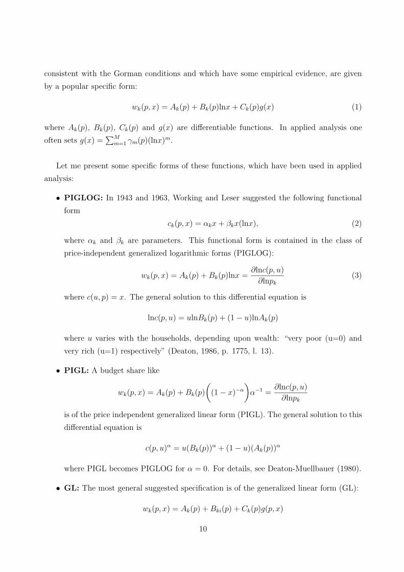
consistent with the Gorman conditions and which have some empirical evidence, are given
by a popular specific form:
wk(p, x) = Ak(p) + Bk(p)lnx + Ck(p)g(x) (1)
where Ak(p), Bk(p), Ck(p) and g(x) are differentiable functions. In applied analysis one
often sets g(x) =∑M
m=1 γm(p)(lnx)m.
Let me present some specific forms of these functions, which have been used in applied
analysis:
• PIGLOG: In 1943 and 1963, Working and Leser suggested the following functional
form
ck(p, x) = αkx + βkx(lnx), (2)
where αk and βk are parameters. This functional form is contained in the class of
price-independent generalized logarithmic forms (PIGLOG):
wk(p, x) = Ak(p) + Bk(p)lnx =∂lnc(p, u)
∂lnpk
(3)
where c(u, p) = x. The general solution to this differential equation is
lnc(p, u) = ulnBk(p) + (1 − u)lnAk(p)
where u varies with the households, depending upon wealth: “very poor (u=0) and
very rich (u=1) respectively” (Deaton, 1986, p. 1775, l. 13).
• PIGL: A budget share like
wk(p, x) = Ak(p) + Bk(p)
((1 − x)−α
)α−1 =
∂lnc(p, u)
∂lnpk
is of the price independent generalized linear form (PIGL). The general solution to this
differential equation is
c(p, u)α = u(Bk(p))α + (1 − u)(Ak(p))α
where PIGL becomes PIGLOG for α = 0. For details, see Deaton-Muellbauer (1980).
• GL: The most general suggested specification is of the generalized linear form (GL):
wk(p, x) = Ak(p) + Bki(p) + Ck(p)g(p, x)
10

where∑
k Ck(p) =∑
k Bki(p) =∑
i Bki(p) = 0 and∑
k Ak(p) = 1. A PIGL budget
share is contained in the GL class. In this special case, set g(p, x) = (1 − x−α)α−1, i.e.
g(p, x) is price independent3.
From these three classes of Engel curves, it is possible to derive some parametric forms
of demand functions, which can be empirically scrutinized:
1. Deaton and Muellbauer (1980) took budget shares of the PIGLOG form and specified
lnAk(p) and lnBk(p) such that
lnc(p, u) = a0 +∑
l
αllnpl + ln1
2
∑l
∑j
γ∗ljlnpklnpj + uβ0Πlp
βl
l
where αs, βs and γ∗st are parameters such that c(p, u) is consistent with utility maxi-
mization theory, i.e. it is linear homogeneous in p. After some calculations one obtains
the almost ideal demand system (AIDS):
wk(p, x) = αk +∑
j
γkjlnpj + βkln(x/P ), (4)
where P is a price index and γkj = 12(γ∗
kj + γ∗jk). Notice that this system has rank two.
For further details, see Deaton-Muellbauer (1980).
2. A quadratic extension of the AIDS is given by Blundell, Pashardes and Weber (1993)
and Banks, Blundell and Lewbel (1997). The latter show that exactly aggregable utility
derived demand systems of rank three must have g(x) = (lnx)2 in (1) and Bk(p) and
Ck(p) cannot both be price independent. Hence their quadratic almost ideal demand
system (QUAIDS) is based on rank three Engel curves of the form
wk(p, x) = Ak(p) + Bk(p)lnx + Ck(p)(lnx)2.
Using information on the functional form of the indirect utility function and using
specific translog forms for the unknown functions, similar to Deaton-Muellbauer (1980),
they obtain the QUAIDS, which is
wk(p, x) = αk +∑
j
γkjlnpj + βkln(x/P1) +λk
P2
(ln(x/P1)
)2
(5)
3As an extension, the function gi(p, x) could also depend on an individual behavior parameter. For
simplicity, I have set this constant equal to one. For further details, see Deaton-Muellbauer (1980).
11

where αs, βs and γst are parameters as in the AIDS, P1 and P2 form indices and λk is
a new parameter, due to the third rank of the demand system.
Up to now I have derived and pointed out two different demand systems, given by (4)
and (5), both of which are consistent with utility maximization theory and commonly used
in applied analysis. Now I will switch to the aggregation framework of demand systems.
It is easy to aggregate these kinds of demand systems, as I will show for the QUAIDS. Taking
into account that i is the index for households i = 1, . . . , n, (5) then becomes
wik(p, xi) = αki +
∑j
γkjlnpj + βkiln(xi/P1) +λki
P2
(ln(xi/P1)
)2
.
The mean expenditure share for good k as defined by
Wk(p, x) =1
n
∑i
wik(p, xi)
can then be written as
Wk(p, x) = meaniαki +∑
j
γkjlnpj + meani
(βkiln(xi/P1)
)+ meani
(λki
P2
(ln(xi/P1)
)2)
which has apparently the same structural form as the individual shares. The reason for
this is its linearity in the household specific parameters. Blundell et al. (1993) extend this
approach by suggesting to write individual behavior parameters αki, βki and λki as a linear
combination of alternative household characteristics ai, like age and sex. The approach of
Banks et al. (1997) points in the same direction. For further details, see their papers. In
a recent survey, Blundell and Stoker (2000) are concerned with impacts of the household
income distribution on aggregate demand. They show that this kind of heterogeneity affects
the shape of rank two and rank three demand systems.
12
3 Behavioral Heterogeneity
Let us now focus on the second theoretical approach, the modelling of behavioral hetero-
geneity, which is quite different to what we have seen in Section 2. For one thing, cancel the
assumptions I made in Section 2. In the following section, I do not state any assumption
about individual behavior of households. I will work with a much wider class of admissible
demand and, therefore, expenditure share functions. Distributions of individual character-
istics and heterogeneous behavior will play an important role. It is shown that structural
properties of aggregate demand can be induced by behavioral heterogeneity and not only by
imposing some regularity conditions on household behavior. This section is based on two
articles: Kneip (1999) and Hildenbrand and Kneip (1999).
Kneip (1999) Kneip considers a continuum of households with expenditure shares w ∈ Wand household characteristics a ∈ AM . Firstly, he states some technical assumptions:
Assumption 2 There exists a continuous density µ(a) : AM �→ [0, 1] for the distribution of
individual characteristics a.
This assumption is restrictive in one way because some of the observable characteristics,
for example age, are discrete numbers. To simplify the theoretical analysis, we assume the
densities are continuous. This does not decrease the generality of the economy. Note that
Kneip only considers a single individual characteristic, M = 1, namely disposable household
income. I therefore here consider an extended framework with more than one individual
characteristic.
Assumption 3 1. For some γ ∈ IR+ and some subspace I ⊂ [0, γ]K, the space of ad-
missible expenditure share functions is a subset of the set V(I) of all functions from
IRK+ × IR+ to I. There exists a Lebesgue measure on I.
2. The space W is large enough such that for any w ∈ W and all ∆ ∈ IRK++, Θ ∈ IRM
+ the
function v satisfying
v(p, x) = w(∆ ∗ p, Θ ∗ a) for all p ∈ IRK++ and a ∈ AM,
is also an element of W. Furthermore, for all p and a the set {w(p, a) ∈ I|w ∈ W} is
Lebesgue measureable.
13
These conditions are of a technical nature. They do not affect an economist’s point of view.
In addition to the previous assumptions we need a precise definition of a probability space
for ν.
Assumption 4 1. The distribution ν is a probability measure on the σ-algebra AW of
W.
2. For every continuous function v : I �→ IR the integral∫
Iv(z)νp,a(dz) is differentiable
with respect to p and a.
The first condition makes use of AW , the smallest σ-algebra of W , containing all sets of the
form A = {w ∈ W|w(p, a) ∈ Jp,a}, where {Jp,a}p,a∈IRK++×AM .
As a consequence of these assumptions, the following integral exists
Wν(p, a) =
∫W×AM
w(p, a)dνµ(a)da.
In other words, one has a convenient tool with which to write the mean expenditure share.
Example 1 Suppose that the budget identity holds for all households. The space I then
restricts to {z ∈ IRK++|
∑Kk=1 zk = 1}. Realizations on I are observable, hence also the
distribution νp,a of the zk’s. Keeping that in mind, the above integral for fixed p, a becomes
Wν(p, a) =
∫{z|z∈I}
zνp,a(dz) =
∫{z|z∈I}
zφp,a(z)dz
where for fixed p, a, νp,a is the k-dimensional distribution of z on I with the density φp,a(z).
For further analysis I also need a precise formulation of demand behavior.
Definition 1 Consider two different households i and j. They possess a similar demand
behavior, if supp,a‖wi(p, a) − wj(p, a)‖2 is small, where ‖ ∗ ‖2 is the Euclidean distance.
Of course, similar demand behavior does not imply similar demand. With this definition
Kneip skilfully uses the relative nature of share functions. For some examples, see Kneip
(1999). Thus, a flat distribution of ν on W can be considered as behavioral heterogeneity. A
uniform distribution can be interpreted as extreme heterogeneity. In other words, extreme
heterogeneity then induces equal probability for equal sized sets. One can express this by
the following relationship, which should hold for all Borel sets J ⊂ I:
νp,a(J) = ν∆∗p,Θ∗a(J)
14
for fixed p and x, where the right hand side is a distance preserving transformation of the
left hand side with (∆, Θ) ∈ IRK++ ×AM. For details, see Kneip (1999).
It is expected that the equation above does not hold, but νp,a(J) ≈ ν∆∗p,Θ∗a(J) for (∆, Θ) ≈(1,1) could be reasonable. In addition, one can equivalently say that for any measurable
subset J ⊂ I the partial derivatives ∂∆rν∆∗p,Θ∗a(J)|(∆,Θ)=(1,1) are close to zero, where r =
1, . . . , K,K + 1, . . . , K + M and ∆K+1 = Θ1, . . . , ∆K+M = ΘM .
Definition 2 Let C(I, [0, γ]) denote the space of all continuous functions from I into [0, γ].
A measure of the structural stability of mean demand is
h(v) = maxrsupp,ahp,a;r(v),
the coefficient of sensitivity, where
hp,a;r(v) = supv∈C(I,[0,γ])
∣∣∣∣∂∆r
(∫I
v(z)ν∆∗p,Θ∗a(dz)
)|(∆,Θ)=(1,1)
∣∣∣∣.The coefficient is small in the case of behavioral heterogeneity and in the case of invariant
demand behavior. This is identified as structural stability.
Definition 3 Mean demand is structurally stable, if
• the household expenditure shares are independent of household characteristics or prices
respectively, or
• the population is very heterogeneous in its behavior.
In addition, the coefficient of sensitivity becomes smaller with a combination of these two
points. For an alternative definition, see Hildenbrand and Kneip (1997) and Hildenbrand
and Kneip (1996). They consider a population over time and conclude that mean demand is
structurally stable if the distributions of household characteristics are invariable over time.
Kneip (1999) proves that a small coefficient of sensitivity implies certain structural properties
of mean demand:
Proposition 1 The Jacobian matrix of mean demand with respect to prices is negative
definite for all prices p ∈ IRK++ if the coefficient of sensitivity h(ν) is sufficiently small and
if there is a constant c > 0 such that∫W wk(p, a)dν ≥ c.
Therefore, the Law of Demand holds for mean demand. In addition, Kneip shows nega-
tive semi-definiteness of the Slutsky substitution matrix of aggregate demand and positive
15
definiteness of the Slutsky income matrix, hence the Slutsky decomposition for utility derived
demand theory holds for the mean demand, if and only if the coefficient is small enough.
We obtain rational mean behavior by a sufficient degree of structural stability.
Example 2 Cobb-Douglas. Suppose that the household demand functions are given by
f ik(p, xi) = βi
kxi/p, where xi denotes the income of each household and∑
k βik = 1 for all i.
There is equivalence of the distribution νp,a and the distribution of β, since wik(p, xi) = βi
k,
and therefore h(ν) = 0.
More generally, Kneip shows that small derivatives of all household budget share functions
imply a small coefficient of sensitivity h(ν).
Hildenbrand and Kneip (1999) The authors derive an index that measures the degree
of behavioral heterogeneity of a population. In addition, they show that structural prop-
erties of mean demand, such as negative definiteness of its Jacobian matrix, are generated
by heterogeneity in the households’ behavior. In contrast to former approaches, i.e. Hilden-
brand (1993) and Kneip (1999), they choose a decomposition of mean demand that requires
less restrictive conditions on individual behavior than the Slutsky decomposition.
Suppose that the population H consists of i = 1, . . . , n households. Each household
possesses a demand function f i depending on income xi > 0 and prices p, i.e. fk(p, ai) :=
f ik(p, xi). The specific behavior of a household is therefore completely described by the
household’s characteristics (f i, xi). The demand function of a household for good k given
prices p and income xi is f ik(p, xi), where k = 1, . . . , K and p ∈ (0,∞)K . Let X denote mean
income of the population H
X =1
n
n∑i=1
xi.
Accordingly, the mean expenditure share for good k is defined as:
Wk(p) :=pk
XFk(p).
Now, let us define Skl(p), the rate of change of Wk(p) with respect to a percentage change
of the price pl as
Skl(p) := ∂λWk(p1, . . . , λpl, . . . , pK)|λ=1 = pl∂plWk(p)
and accordingly for wik(p, xi) one obtains
sikl(p, xi) := ∂λw
ik(p1, . . . , λpl, . . . , pK , xi)|λ=1 = pl∂pl
wik(p, xi).
16
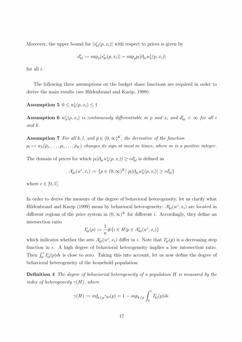
Moreover, the upper bound for |sikl(p, xi)| with respect to prices is given by
dikl := supp|si
kl(p, xi)| = supppl|∂plwi
k(p, xi)|
for all i.
The following three assumptions on the budget share functions are required in order to
derive the main results (see Hildenbrand and Kneip, 1999):
Assumption 5 0 ≤ wik(p, xi) ≤ 1
Assumption 6 wik(p, xi) is continuously differentiable in p and xi and di
kl < ∞ for all i
and k.
Assumption 7 For all k, l, and p ∈ (0,∞)K, the derivative of the function
pl �→ wk(p1, . . . , pl, . . . , pK) changes its sign at most m times, where m is a positive integer.
The domain of prices for which pl|∂plwi
k(p, xi)| ≥ εdikl is defined as
Aεkl(w
i, xi) := {p ∈ (0,∞)K | pl|∂plwi
k(p, xi)| ≥ εdikl}
where ε ∈ [0, 1].
In order to derive the measure of the degree of behavioral heterogeneity, let us clarify what
Hildenbrand and Kneip (1999) mean by behavioral heterogeneity: Aεkl(w
i, xi) are located in
different regions of the price system in (0,∞)K for different i. Accordingly, they define an
intersection ratio
Iεkl(p) :=
1
n#{i ∈ H|p ∈ Aε
kl(wi, xi)}
which indicates whether the sets Aεkl(w
i, xi) differ in i. Note that Iεkl(p) is a decreasing step
function in ε. A high degree of behavioral heterogeneity implies a low intersection ratio.
Then∫ 1
0Iεkl(p)dε is close to zero. Taking this into account, let us now define the degree of
behavioral heterogeneity of the household population:
Definition 4 The degree of behaviorial heterogeneity of a population H is measured by the
index of heterogeneity γ(H), where
γ(H) := infk,l,pγkl(p) = 1 − supk,l,p
∫ 1
0
Iεkl(p)dε.
17
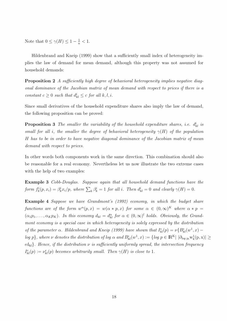
Note that 0 ≤ γ(H) ≤ 1 − 1n
< 1.
Hildenbrand and Kneip (1999) show that a sufficiently small index of heterogeneity im-
plies the law of demand for mean demand, although this property was not assumed for
household demands:
Proposition 2 A sufficiently high degree of behavioral heterogeneity implies negative diag-
onal dominance of the Jacobian matrix of mean demand with respect to prices if there is a
constant c ≥ 0 such that dikl ≤ c for all k, l, i.
Since small derivatives of the household expenditure shares also imply the law of demand,
the following proposition can be proved:
Proposition 3 The smaller the variability of the household expenditure shares, i.e. dikl is
small for all i, the smaller the degree of behavioral heterogeneity γ(H) of the population
H has to be in order to have negative diagonal dominance of the Jacobian matrix of mean
demand with respect to prices.
In other words both components work in the same direction. This combination should also
be reasonable for a real economy. Nevertheless let us now illustrate the two extreme cases
with the help of two examples:
Example 3 Cobb-Douglas. Suppose again that all household demand functions have the
form f ik(p, xi) = βi
kxi/p, where∑
k βik = 1 for all i. Then di
kl = 0 and clearly γ(H) = 0.
Example 4 Suppose we have Grandmont’s (1992) economy, in which the budget share
functions are of the form wα(p, x) = w(α ∗ p, x) for some α ∈ (0,∞)K where α ∗ p =
(α1p1, . . . , αKpK). In this economy dkl = dαkl for α ∈ (0,∞)l holds. Obviously, the Grand-
mont economy is a special case in which heterogeneity is solely expressed by the distribution
of the parameter α. Hildenbrand and Kneip (1999) have shown that Iεkl(p) = ν{Bε
kl(w1, x)−
log p}, where ν denotes the distribution of log α and Bεkl(w
1, x) := {log p ∈ IRK| |∂log plw1
k(p, x)| ≥εdkl}. Hence, if the distribution ν is sufficiently uniformly spread, the intersection frequency
Iεkl(p) := νε
kl(p) becomes arbitrarily small. Then γ(H) is close to 1.
18

4 Summary and Criticism
Two different approaches to the modelling of mean demand have been surveyed. The classic,
utility derived, approach uses well known results of microeconomics. There is a wide range
of contributions in the literature dealing with this topic. In applied analysis, the resulting
demand systems are estimable with parametric statistical methods. This has often been
done, in many cases the systems fitted the data well. However, there are methodological
problems imbedded in this approach. To state restrictive assumptions on the behavior of
the households is difficult to justify. Moreover, it seems unrealistic that demand decisions of
households are made independently of individual characteristics, except income. As a matter
of fact there are some articles allowing for individual components but these approaches are
artificial because they only exploit the freedom given by Gorman’s Engel curve specification,
for some differentiable functions. Nevertheless, the fit of aggregate data for Gorman form
Engel curves can be considered a stylized fact. In contrast this fit at the macro level does
not allow welfare analysis at the micro level as in Banks et al. (1997). Analyses of this
kind and expressions of the form ”richer people have higher utility than poorer people”, as in
Deaton (1986) show the methodological dilemma of the classic approach at the micro level.
Nevertheless, the classical approach can be used as the theoretical foundation for empirical
analysis at the macro level. However, semiparametric estimation seems to be a good com-
promise between an adequate rate of convergence of the estimators and a moderate risk of
misspecification.
The second approach presented allows for more generality at the micro level. Here, it
is not as necessary to describe completely each individual in order to explain structures of
aggregate demand, as it is in the first approach. Indeed, it is possible to achieve compatible
results for mean demand, e.g. if the sensitivity coefficient or the index of heterogeneity is
small, without making restrictive assumptions on the behavior of the households, e.g. re-
strictions on the class of feasible expenditure share functions. As a matter of fact, it is
difficult to scrutinize how structurally stable mean demand is. It is impossible to find out
empirically how large the index of heterogeneity is for a given population. Moreover, behav-
ioral heterogeneity is not uniquely defined by the authors.
There are only a few contributions treating the empirical evidence of this approach, e.g.
Hildenbrand and Kneip (1996, 1999). The econometric modelling of behavioral heterogeneity
is still in the first steps of development. Due to an increase of computational power during
19

the past few years and significant progress in non- and semiparametric statistics, there are
devices and tools now available which can play a key role in econometric modelling of be-
havioral heterogeneity in demand theory.
Finally, I conclude that from a theoretical point of view, there is no contradiction in the
results of the two approaches presented. The statistician should use the advantages of both
in order to build a model to be estimated.
20
References
[1] Banks, J. and Blundell, R. and Lewbel, A. (1997). Quadratic Engel Curves and Consumer
Demand. The Review of Economics and Statistics, Vol. LXXIX (No. 4): 527–539.
[2] Blundell, R. and Pashardes, P. and Weber, G. (1993). What do we Learn about Consumer
Demand Patterns from Micro Data. American Economic Review, Vol. 83 (No. 3): 570–597.
[3] Blundell, R. and Stoker, T. (2000). Models of Aggregate Economic Relationships that
account for Heterogeneity. Handbook of Econometrics V, North-Holland, Amsterdam.
[4] Deaton, A (1986). Demand Analysis. Handbook of Econometrics III, North-Holland,
Amsterdam.
[5] Deaton, A and Muellbauer, J. (1980). An almost ideal demand system. American
Economic Review, Vol. 70: 312-336.
[6] Grandmont, J.M. (1992). Transformation of the Commodity Space, Behavioral Hetero-
geneity, and the Aggregation Problem. Journal of Economic Theory, 57(1): 1–35.
[7] Gorman, W. (1981). Some Engel Curves. In: The Theory and Measurement of Consumer
Behavior, Angus Deaton (Ed.), Cambridge University Press, Cambridge.
[8] Hildenbrand, W. (1993). Market Demand. Princeton University Press, Princeton.
[9] Hildenbrand, W. and Kneip, A. (1996). Modelling Aggregate Consumption Expenditure
and Income Distribution Effects. SFB 303 Discussion Paper No. A-510, Universitat Bonn.
[10] Hildenbrand, W. and Kneip, A. (1999). Demand Aggregation under Structural Stability.
Journal of Mathematical Economics, 31: 81-109.
[11] Hildenbrand, W. and Kneip, A. (1999). On Behavioral Heterogeneity. SFB 303 Discus-
sion Paper No. A-589, Universitat Bonn.
[12] Kneip, A. (1999). Behavioral Heterogeneity and Structural Properties of Aggregate
Demand. Journal of Mathematical Economics, 31: 49-74.
[13] Leser C.E.V. (1963). Forms of Engel-Functions. Econometrica, Vol. 31: 694-703.
[14] Mas Colell, A., Whinston, Green (1995). Microeconomic Theory. Oxford University
Press, Oxford.
21

[15] Working, H. (1943). Statistical Laws of Family Expenditure. Journal of the American
Statistical Association, Vol. 38: 43-56.
22
Essay 2
A Note on Behavioral Heterogeneity
and Aggregation
April 22, 2002
Abstract
The purpose of this note is to investigate how aggregation of households affects the
variation of the index of heterogeneity as recently defined in Hildenbrand and Kneip
(1999). We show the degree of behavioral heterogeneity of an entire population is at
least as high as the smallest degree of behavioral heterogeneity of some disjoint sub-
population. We further derive conditions under which aggregation increases the degree
of behavioral heterogeneity. Finally, we show that aggregation always weakly increases
the degree of behavioral heterogeneity. Therefore we offer a theoretical framework that
helps to answer the question of how the structural properties of aggregate demand are
obtained due to aggregation.
1 Introduction
In a recent paper Hildenbrand and Kneip (1999) develop an index that measures the degree
of behavioral heterogeneity of a population. It is well known that structural properties of
aggregate demand, such as negative definiteness of the Jacobian matrix, are generated by
heterogeneity in household’s behavior. In particular, Hildenbrand and Kneip (1999) show
that a sufficiently large index implies the law of demand for mean demand. In contrast to
former approaches, i.e. Hildenbrand (1993) and Kneip (1999), these authors have chosen
a decomposition of aggregate demand that requires less restrictive conditions on individ-
ual behavior than the Slutsky decomposition. In addition, their work is a generalization of
Grandmont’s (1992) economy.
The aim of this note is to derive further properties of the index of heterogeneity. We
mainly focus on the question of what happens to the structural properties of mean demand if
we aggregate subpopulations, i.e. we investigate the impact of aggregation on the degree of
behavioral heterogeneity. We present three results: Firstly, aggregation never decreases the
degree of behavioral heterogeneity. In other words, the degree of behavioral heterogeneity at
the aggregate level is higher than the lowest degree of behavioral heterogeneity of arbitrary
disjoint subpopulation. Secondly, we show that the degree of behavioral heterogeneity at the
aggregate level can be either greater or smaller than the maximal degree of heterogeneity of
all subpopulations. Since we intend to investigate the impacts of behavioral heterogeneity
on the structural properties of aggregate demand, we derive conditions for generating het-
erogeneity due to aggregation. Thirdly, and finally, we show that aggregation always weakly
generates heterogeneity. In other words, aggregation leads to a higher degree of behavioral
heterogeneity at the aggregate level when compared to the weighted average of arbitrary
disjoint subpopulations.
Notation We use the same notation as in Hildenbrand and Kneip (1999).
Suppose that every household h ∈ H with income xh > 0 has a demand function fh. The
specific behavior of a household is completely described by the household’s characteristics
(fh, xh). The demand function of a household for good i given prices p and xh is fhi (p, xh),
where i = 1, . . . , l and p ∈ (0,∞)l. Let X denote mean income of the population and let
F (p) :=1
#H
∑h∈H
fh(p, xh) ∈ IRl+
24
denote mean demand. The household expenditure share is defined as
whi (p, xh) :=
pi
xhfh
i (p, xh)
and analogously we obtain the mean expenditure share for good i:
Wi(p) :=pi
XFi(p).
Now, consider the rate of change of Wi(p) and whi (p, xh) with respect to a percentage change
of the price pj which is defined as
Sij(p) := ∂λWi(p1, . . . , λpj, . . . , pl)|λ=1 = pj∂pjWi(p)
and
shij(p, x
h) := ∂λwhi (p1, . . . , λpj, . . . , pl, x
h)|λ=1 = pj∂pjwh
i (p, xh).
Moreover, the upper bound for |shij(p, x
h)| with respect to prices is given by
dhij := supp|sh
ij(p, xh)| = supppj|∂pj
whi (p, xh)|
for all h ∈ H.
The following three assumptions on the budget share functions are required to derive the
following results, see Hildenbrand and Kneip (1999):
Assumption 1 0 ≤ wi(p, x) ≤ 1
Assumption 2 w(p, x) is continuously differentiable in p and x and dhij < ∞ for all h ∈ H.
Assumption 3 For all i, j, and p ∈ (0,∞)l, the derivative of the function
pj �→ wi(p1, . . . , pj, . . . , pl) changes its sign at most m times, where m is a positive integer.
The domain of prices for which pj|∂pjwh
i (p, xh)| ≥ εdhij is defined as
Aεij(w
h, xh) := {p ∈ (0,∞)l| pj|∂pjwh
i (p, xh)| ≥ εdhij}
where ε ∈ [0, 1].
In order to derive the definition of the degree of behavioral heterogeneity, let us clarify
what it means in the framework of Hildenbrand and Kneip (1999): Aεij(w
h, xh) are located
25
in different regions of the price system in (0,∞)l for different h. Accordingly, they define an
intersection ratio
Iεij(p) :=
1
#H#{h ∈ H|p ∈ Aε
ij(wh, xh)}
which indicates whether the sets Aεij(w
h, xh) differ in h. Note that Iεij(p) is a decreasing
step function in ε. A high degree of behavioral heterogeneity implies a low intersection
ratio. Then∫ 1
0Iεij(p)dε is close to zero. Taking this into account we can define the degree of
behavioral heterogeneity of the household population H as
γ(H) := infi,j,pγij(p) = 1 − supi,j,p
∫ 1
0
Iεij(p)dε.
Note that 0 ≤ γ(H) ≤ 1 − 1#H
< 1.
In addition, define Gεij(p) := 1 − Iε
ij(p). Then
Gεij(p) =
1
#H#{h ∈ H||sh
ij(p, xh)| < εdh
ij}
is the cumulative distribution function of |shij(p, x
h)|/dhij.
2 Behavioral Heterogeneity and Aggregation
In this section, we derive some properties of the index of heterogeneity, while taking into
account the aggregation over subpopulations.
Aggregation Over Subpopulations. Consider m = 1, . . . , k nonempty subpopulations
of H with⋃k
m=1Hm = H, where
⋃denotes the union of disjoint sets. The disjoint subpop-
ulations are allowed to be of arbitrary size and arbitrary composition.
Definition 1 Aggregation reduces heterogeneity as measured by γ, if
γ(H) < infmγ(Hm)
is true.
Definition 2 Aggregation increases heterogeneity as measured by γ, if
γ(H) ≥ supmγ(Hm)
is true.
26

Proposition 1 Aggregation cannot reduce the degree of behavioral heterogeneity as measured
by γ, i.e. for every H and {Hm}m=1,...,k such that⋃k
m=1Hm = H it follows
γ(H) ≥ infmγ(Hm).
Proof. It suffices to prove the proposition for k = 2, since Hk ∪(⋃k−1
m=1Hm
)= H.
Suppose we have two subpopulations m and n and assume without loss of generality that
γ(Hm) ≤ γ(Hn). Then,
Iεij(p) =
1
#Hm + #Hn#{h ∈ Hm ∪ Hn|p ∈ Aε
ij(wh, xh)}
=1
#Hm + #Hn
(#HmIεm
ij (p) + #HnIεnij (p)
)(1)
≤ sup{Iεmij (p), Iεn
ij (p)}
for ε ∈ [0, 1], where
Iεmij (p) :=
1
#Hm#{h ∈ Hm|p ∈ Aε
ij(wh, xh)}.
Applying this inequality gives
1 − γij(p) =
∫ 1
0
Iεij(p)dε ≤
∫ 1
0
sup{Iεmij (p), Iεn
ij (p)}dε ≤ 1 − inf{γmij (p), γn
ij(p)}⇔ γij(p) ≥ inf{γm
ij (p), γnij(p)}
for all i, j and p ∈ (0,∞)l, which proves Proposition 1. �
Note, however, that we can neither infer from Proposition 1 that an expansion of the pop-
ulation by an additional household does not lead to a decrease in the index of heterogeneity
nor that γ(H) < supmγ(Hm) holds. More generally, we ask whether γ(H) ≥ supmγ(Hm)
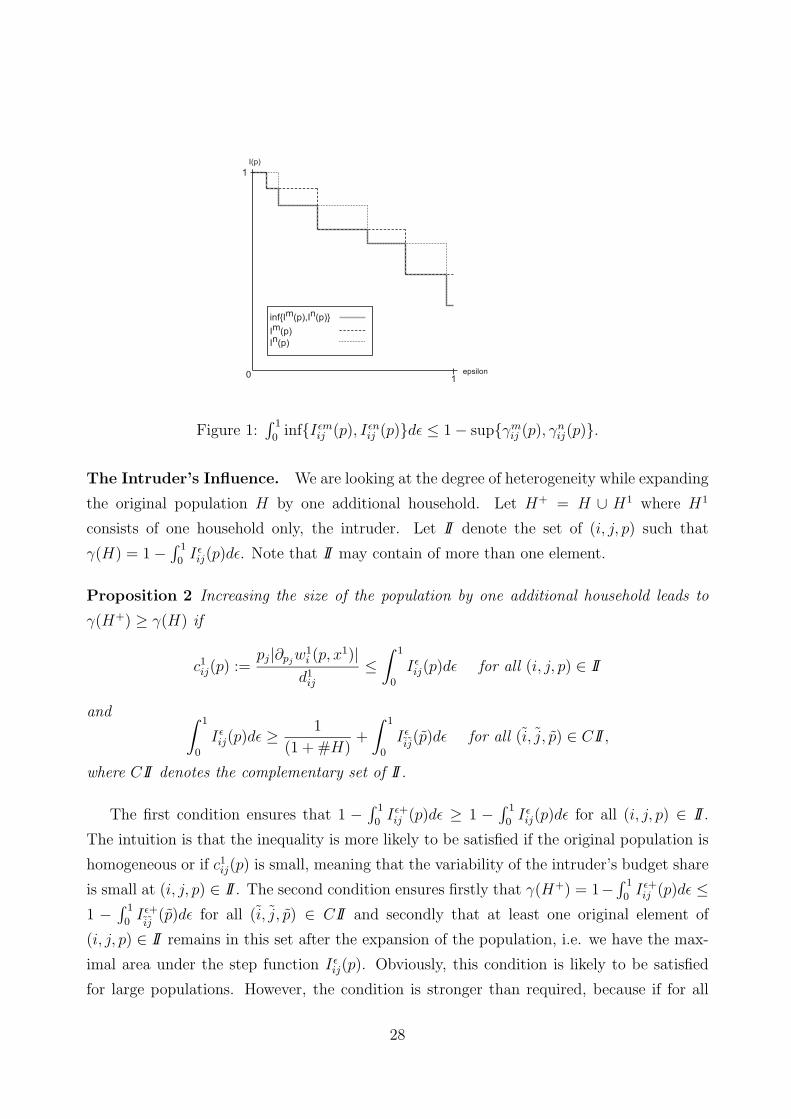
may occur. We show that this inequality does not hold in general: because of equation (1)
one can infer Iεij(p) ≥ inf{Iεm
ij (p), Iεnij (p)} (see Figure 1). Therefore
1 − γij(p) =
∫ 1
0
Iεij(p)dε ≥
∫ 1
0
inf{Iεmij (p), Iεn
ij (p)}dε ≤ 1 − sup{γmij (p), γn
ij(p)},
which is not a unique relation.
The next propositions shed light on this point. Proposition 2 looks at an expansion of
the original population by an additional household, while Proposition 3 considers the general
case when aggregating subpopulations of arbitrary size.
27
inf{Im(p),In(p)} Im(p)In(p)
1
1
0
I(p)
epsilon
Figure 1:∫ 1
0inf{Iεm
ij (p), Iεnij (p)}dε ≤ 1 − sup{γm
ij (p), γnij(p)}.
The Intruder’s Influence. We are looking at the degree of heterogeneity while expanding
the original population H by one additional household. Let H+ = H ∪ H1 where H1
consists of one household only, the intruder. Let II denote the set of (i, j, p) such that
γ(H) = 1 − ∫ 1
0Iεij(p)dε. Note that II may contain of more than one element.
Proposition 2 Increasing the size of the population by one additional household leads to
γ(H+) ≥ γ(H) if
c1ij(p) :=
pj|∂pjw1
i (p, x1)|
d1ij
≤∫ 1
0
Iεij(p)dε for all (i, j, p) ∈ II
and ∫ 1
0
Iεij(p)dε ≥ 1
(1 + #H)+
∫ 1
0
Iεij(p)dε for all (i, j, p) ∈ CII,
where CII denotes the complementary set of II.
The first condition ensures that 1 − ∫ 1
0Iε+ij (p)dε ≥ 1 − ∫ 1
0Iεij(p)dε for all (i, j, p) ∈ II.
The intuition is that the inequality is more likely to be satisfied if the original population is
homogeneous or if c1ij(p) is small, meaning that the variability of the intruder’s budget share
is small at (i, j, p) ∈ II. The second condition ensures firstly that γ(H+) = 1−∫ 1
0Iε+ij (p)dε ≤
1 − ∫ 1
0Iε+ij
(p)dε for all (i, j, p) ∈ CII and secondly that at least one original element of
(i, j, p) ∈ II remains in this set after the expansion of the population, i.e. we have the max-
imal area under the step function Iεij(p). Obviously, this condition is likely to be satisfied
for large populations. However, the condition is stronger than required, because if for all
28

(i, j, p) ∈ CII : c1ij(p) ≤ ∫ 1
0Iεij(p)dε, then
∫ 1
0Iε+ij
(p)dε ≤ ∫ 1
0Iεij(p)dε. In those cases we do not
require the second condition. However, we use the stronger version of the second condition.
The first condition is also satisfied if
c1ij(p) ≤ infh∈H
pj|∂pjwh
i (p, xh)|dh
ij
,
meaning that the intruder needs to have less relative variability of the budget share for
(i, j, p) ∈ II than every household of the original population. In fact, this condition is
stronger than the first one.
Let us prove Proposition 2 and illustrate it with the help of three examples.
Proof. The inequality γ(H+) ≥ γ(H) corresponds to supi,j,p
∫ 1
0Iε+ij (p) ≤ supi,j,p
∫ 1
0Iεij(p).
In the Part A we prove the proposition for the strong version of the first condition. In Part
B we show the general result.
A Since Gεij(p) is the cumulative distribution function of |si(p,xh)|
dhij
, we have for all (i, j, p) ∈ II
that Gε+ij (p) ≥ Gε
ij(p) for ε ∈ [0, 1], if c1ij(p) ≤ infh∈H
pj |∂pj whi (p,xh)|
dhij
and therefore Iε+ij (p) −
Iεij(p) ≤ 0. Using the properties of first order stochastic dominance (Lemma 2 in the
appendix) leads to γ+ij (p) ≥ γij(p) for all (i, j, p) ∈ II. In order to ensure
∫ 1
0Iεij(p)dε ≥∫ 1
0Iε+ij
(p)dε for all (i, j, p) ∈ II and all (i, j, p) ∈ CII we need the second condition, since
1(1+#H)
≥ supi,j,p
(∫ 1
0Iε+ij (p)dε − ∫ 1
0Iεij(p)dε
)for all (i, j, p) ∈ II ∪ CII.
B One can show that
Iε+ij (p) − Iε
ij(p) =
11+#H
(1 − Iε
ij(p))
if|w1
i (p,x1)|d1
ij≥ ε
−Iεij(p)
1+#Hotherwise
In order to obtain ∫ 1
0
Iε+ij (p) − Iε
ij(p)dε ≤ 0,
we need1
1 + #H
(∫ c1ij(p)
0
1dε −∫ c1ij(p)
0
Iεijdε −
∫ 1
c1ij(p)
Iεij(p)dε
)≤ 0
and therefore1
1 + #H
(c1ij(p) −
∫ 1
0
Iεij(p)dε
)≤ 0
29
for all (i, j, p) ∈ II such that γ(H) = 1− ∫ 1
0Iεij(p)dε. Using
∫ 1
0Iεij(p)dε−∫ 1
0Iεij(p)dε ≥ 1
(1+#H)
for all (i, j, p) ∈ CII proves the proposition. �
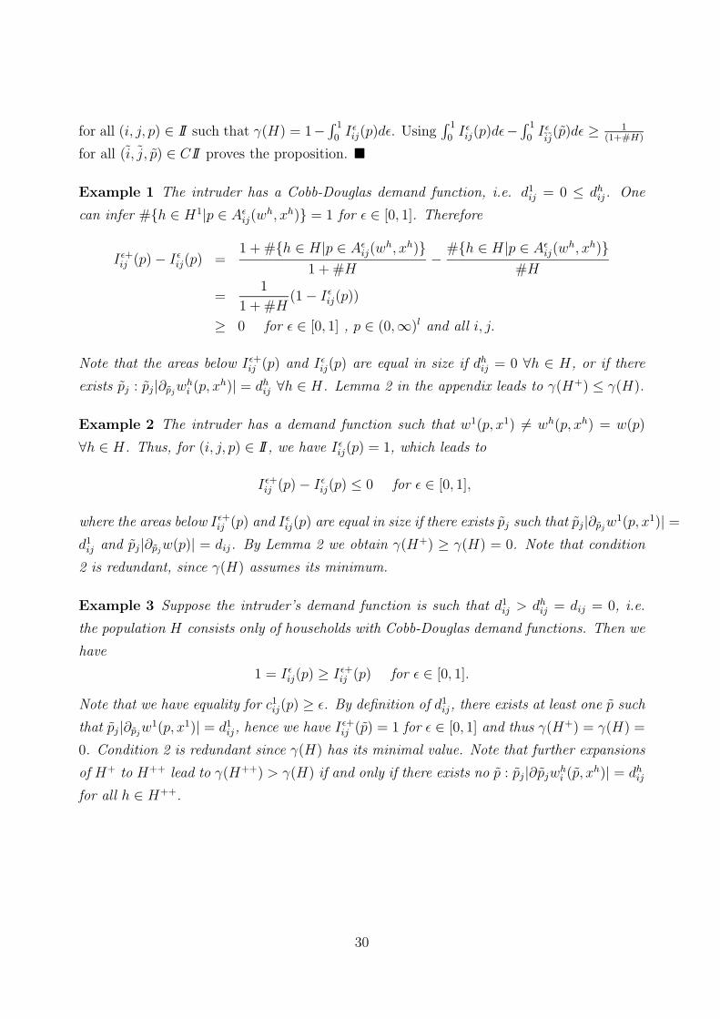
Example 1 The intruder has a Cobb-Douglas demand function, i.e. d1ij = 0 ≤ dh
ij. One
can infer #{h ∈ H1|p ∈ Aεij(w
h, xh)} = 1 for ε ∈ [0, 1]. Therefore
Iε+ij (p) − Iε
ij(p) =1 + #{h ∈ H|p ∈ Aε
ij(wh, xh)}
1 + #H− #{h ∈ H|p ∈ Aε
ij(wh, xh)}
#H
=1
1 + #H(1 − Iε
ij(p))
≥ 0 for ε ∈ [0, 1] , p ∈ (0,∞)l and all i, j.
Note that the areas below Iε+ij (p) and Iε
ij(p) are equal in size if dhij = 0 ∀h ∈ H, or if there
exists pj : pj|∂pjwh
i (p, xh)| = dhij ∀h ∈ H. Lemma 2 in the appendix leads to γ(H+) ≤ γ(H).
Example 2 The intruder has a demand function such that w1(p, x1) = wh(p, xh) = w(p)
∀h ∈ H. Thus, for (i, j, p) ∈ II, we have Iεij(p) = 1, which leads to
Iε+ij (p) − Iε
ij(p) ≤ 0 for ε ∈ [0, 1],
where the areas below Iε+ij (p) and Iε
ij(p) are equal in size if there exists pj such that pj|∂pjw1(p, x1)| =
d1ij and pj|∂pj
w(p)| = dij. By Lemma 2 we obtain γ(H+) ≥ γ(H) = 0. Note that condition
2 is redundant, since γ(H) assumes its minimum.
Example 3 Suppose the intruder’s demand function is such that d1ij > dh
ij = dij = 0, i.e.
the population H consists only of households with Cobb-Douglas demand functions. Then we
have
1 = Iεij(p) ≥ Iε+
ij (p) for ε ∈ [0, 1].
Note that we have equality for c1ij(p) ≥ ε. By definition of d1
ij, there exists at least one p such
that pj|∂pjw1(p, x1)| = d1
ij, hence we have Iε+ij (p) = 1 for ε ∈ [0, 1] and thus γ(H+) = γ(H) =
0. Condition 2 is redundant since γ(H) has its minimal value. Note that further expansions
of H+ to H++ lead to γ(H++) > γ(H) if and only if there exists no p : pj|∂pjwhi (p, xh)| = dh
ij
for all h ∈ H++.
30
Increasing Heterogeneity Due to Aggregation Let us generalize Proposition 2. Sup-
pose H =⋃k
m=1Hm and let supmγ(Hm) =: γ(Hn). In addition, let II be the set of (i, j, p)
such that γ(Hn) = 1 − ∫ 1
0Iεnij (p)dε.
Proposition 3 Aggregation increases the degree of behavioral heterogeneity as measured by
γ, i.e. γ(H) ≥ supmγ(Hm), if the following conditions hold:∫ 1
0
Iεmij (p)dε ≤
∫ 1
0
Iεnij (p)dε
for all (i, j, p) ∈ II and m = 1, . . . , k and∫ 1
0
Iεnij (p)dε −
∫ 1
0
Iεnij
(p)dε ≥ #H − #Hn
#H
for all (i, j, p) ∈ II and for all (i, j, p) ∈ CII such that∫ 1
0
Iεmij
(p)dε ≥∫ 1
0
Iεnij
(p)dε.
Proof. The proof follows the same reasoning as in the proof of Proposition 2. The first
condition implies ∫ 1
0
Iεij(p)dε ≤
∫ 1
0
Iεnij (p)dε
for all (i, j, p) ∈ II. Let CII = ∪2i=1CIIi, where (i, j, p) ∈ CII1 if
∫ 1
0Iεmij
(p)dε ≤ Iεmij
(p)dε ≤∫ 1
0Iεnij (p)dε and (i, j, p) ∈ CII2 if
∫ 1
0Iεmij
(p)dε ≥ Iεmij
(p)dε ≤ ∫ 1
0Iεnij (p)dε. Therefore we have
∫ 1
0
Iεij(p)dε ≤
∫ 1
0
Iεmij
(p)dε
for all (i, j, p) ∈ CII1 and ∫ 1
0
Iεij(p)dε ≥
∫ 1
0
Iεmij
(p)dε
for all (i, j, p) ∈ CII2. Thus, the second condition ensures∫ 1
0Iεij(p)dε ≥ Iε
ij(p)dε for all
(i, j, p) ∈ II and all (i, j, p) ∈ CII2, since supi,j,p
(∫ 1
0Iεij(p) − Iεm
ij (p)dε)
≤ #H−#Hm
#Hfor all
m, i, j and p ∈ (0,∞)l. Hence the set of (i, j, p) such that γ(H) = 1− ∫ 1
0Iεijdε might consist
of elements of II, CII1 and CII2. �
The first condition of Proposition 3 implies that for all (i, j, p) ∈ II the heterogeneity of
subpopulation n has to be the lowest. The second condition says that for subpopulation
n the largest expanding area below the step function has to be smaller than the largest
31

diminishing area minus the largest possible size of variation. The second condition is more
likely to be satisfied if #Hn is large compared to the rest of the population.
The following examples might help in illustrating Proposition 3.
Example 4 Suppose we have two homogeneous subpopulations H1 and H2, where H1 con-
sists only of households with Cobb-Douglas demand functions, i.e. for all h ∈ H1 we have
dhij = 0, and for all h ∈ H2 we have wh(p, xh) = w(p), i.e. dh
ij = dij ≥ 0. Therefore, we have
γ(H1) = γ(H2) = 0 and, as is shown in Example 3, we obtain γ(H) = 0.
Example 5 Suppose we have two homogeneous subpopulations m = 1, 2, where Hm consists
of households with demand functions such that wh(p, xh) = wm(p). Therefore for all h ∈ Hm
we have dhij = dm
ij ≥ 0. We conclude γ(H) > 0 if II1 ∩ II2 = ∅, and γ(H) = 0 otherwise,
where IIm denotes the set of (i, j, p) such that γ(Hm) = 1 − ∫ 1
0Iεmij (p)dε.
Example 6 Suppose we have the Grandmont economy in which the budget share functions
are to be taken of the form wα(p, x) = w(α ∗ p, x) for some α ∈ (0,∞)l, where α ∗ p =
(α1p1, . . . , αlpl). It is well known that dij = dαij for α ∈ (0,∞)l. Hildenbrand and Kneip
(1999) have shown that Iεij(p) = ν{Bε
ij(w1, x) − log p}, where ν denotes the distribution of
log α and Bεij(w
1, x) := {log p ∈ IRl| |∂log pjw1
i (p, x)| ≥ εdij}. Hence, if the distribution ν is
sufficiently uniformly spread, the intersection frequency Iεij(p) := νε
ij(p) becomes arbitrarily
small. Obviously, the Grandmont economy is a special case in which heterogeneity is solely
expressed by the distribution of the parameter α. Let νm denote the distribution of log α for
subpopulation m. Then, the distribution of the entire population is a mixture distribution,
i.e. we have
log α ∼∑m
#Hm
#Hνm
for all m. Then, γ(H) ≥ supmγ(Hm) corresponds to
supi,j,p
∫ 1
0
νεij(p)dε ≤ infmsupi,j,p
∫ 1
0
νεmij (p)dε.
Consequently, the conditions of Proposition 3 immediately apply. Using this concept, in-
creasing heterogeneity due to aggregation corresponds to a mixed distribution ν that is more
uniformly spread than every νm.
32
Weakly Increasing Heterogeneity. Now, we look at a weaker definition of increasing
heterogeneity. Since Proposition 2 and Proposition 3 involve complicated conditions, this
may allow for more intuitive results. We use a concept that compares the degree of hetero-
geneity on average.
Definition 3 Aggregation weakly increases heterogeneity, as measured by γ, if
γ(H) ≥k∑
m=1
#Hm
#Hγ(Hm)
is true.
Before presenting the result by a proposition, we state a lemma.
Lemma 1 For all i, j and p ∈ (0,∞), γij(p) is an element of a convex set. The lower bound
is infmγmij (p) and the upper bound is supmγm
ij (p), where all nonempty subpopulations Hm are
disjoint and H =⋃k
m=1Hm for every positive integer k ≤ #H.
Proof. We have to prove that γij(p) ∈ [infmγmij (p), supmγm
ij (p)] for all i, j and p ∈ (0,∞).
For a fixed ε, one can infer from the definition of Iεij(p) that
Iεij(p) =
k∑m=1
#Hm
#HIεmij (p),
which is a convex combination of Iεmij (p) over m = 1, . . . , k. By rearranging, it follows
immediately that
γij(p) := 1 −∫ 1
0
Iεij(p)dε = 1 −
k∑m=1
#Hm
#H
∫ 1
0
Iεmij (p)dε,
which is evidently a convex combination of 1− supm
∫ 1
0Iεmij (p)dε and 1− infm
∫ 1
0Iεmij (p)dε. �
Now we ask whether γ(H) ≥ ∑km=1
#Hm
#Hγ(Hm) holds. Preliminarily, this inequality is
likely to be satisfied if all γ(Hm) are very small, which corresponds to very homogeneous
subpopulations, or if γ(H) is close to one. The next proposition provides an unambiguous
answer.
Proposition 4 Aggregation weakly generates heterogeneity as measured by γ.
33
Before we provide some intuition, let us prove the proposition.
Proof.
infi,j,pγij(p) ≥ 1 − supi,j,p
k∑m=1
#Hm
#H
∫ 1
0
Iεmij (p)dε
≥ 1 −k∑
m=1
#Hm
#Hsupi,j,p
∫ 1
0
Iεmij (p)dε
=k∑
m=1
#Hm
#H
(1 − supi,j,p
∫ 1
0
Iεmij (p)dε
)
=k∑
m=1
#Hm
#Hinfi,j,pγ
mij (p)
We remark that the first inequality is due to Lemma 1. �
Intuitively, γ(H) is the smallest weighted average over all γmij (p) with respect to (i, j, p)
due to γ(H) := infi,j,pγij(p), while∑k
m=1#Hm
#Hγ(Hm) is the weighted average over infi,j,pγ
mij (p).
Note, the fact that Proposition 4 includes Proposition 1 as a weak increase in heterogeneity
rules out a decrease in heterogeneity as defined in Definition 1.
One can infer that the separation of the population into homogeneous subgroups affects
the structural properties of mean demand. Then we have on average less behavioral hetero-
geneity and we therefore may lose the monotonicity property of mean demand.
Proposition 1 and Proposition 4 are in accordance with results from Kneip (1999). He
proves that the coefficient of sensitivity, a measure of structural stability of a population,
does not decrease on average when aggregating subpopulations. In general, a small coefficient
of sensitivity corresponds either to high behavioral heterogeneity of the population or to low
variability in the demand behavior of households.
34
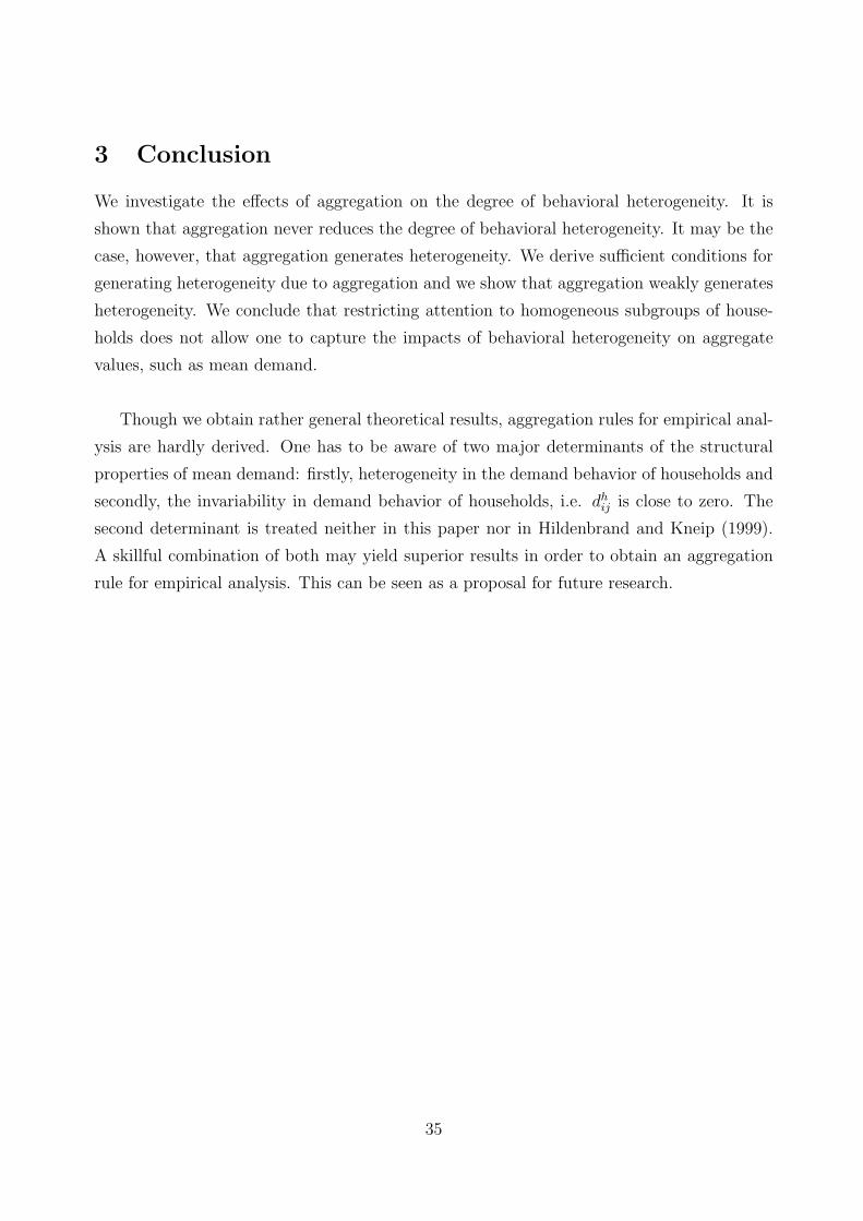
3 Conclusion
We investigate the effects of aggregation on the degree of behavioral heterogeneity. It is
shown that aggregation never reduces the degree of behavioral heterogeneity. It may be the
case, however, that aggregation generates heterogeneity. We derive sufficient conditions for
generating heterogeneity due to aggregation and we show that aggregation weakly generates
heterogeneity. We conclude that restricting attention to homogeneous subgroups of house-
holds does not allow one to capture the impacts of behavioral heterogeneity on aggregate
values, such as mean demand.
Though we obtain rather general theoretical results, aggregation rules for empirical anal-
ysis are hardly derived. One has to be aware of two major determinants of the structural
properties of mean demand: firstly, heterogeneity in the demand behavior of households and
secondly, the invariability in demand behavior of households, i.e. dhij is close to zero. The
second determinant is treated neither in this paper nor in Hildenbrand and Kneip (1999).
A skillful combination of both may yield superior results in order to obtain an aggregation
rule for empirical analysis. This can be seen as a proposal for future research.
35
0 0.1 0.2 0.3 0.4 0.5 0.6 0.7 0.8 0.9 10
0.1
0.2
0.3
0.4
0.5
0.6
0.7
0.8
0.9
1
G
epsilon
G*(p): __ __ G(p) : _____
Figure 2: Gεij(p) first order stochastically dominates Gε∗
ij (p).
Appendix
Lemma 2 Consider two populations H and H∗ such that Iε∗ij (p) − Iε
ij(p) ≤ 0 for ε ∈ [0, 1].
Then we have
γ∗ij(p) − γij(p) ≥ 0.
Proof. For ε ∈ [0, 1] we have
Iε∗ij (p) ≤ Iε
ij(p) ⇔ Gε∗ij (p) ≥ Gε
ij(p).
We know that Gεij(p) = 1−Iε
ij(p) is the cumulative distribution function of|sh
ij(p,xh)|dh
ij, so Gε
ij(p)
first order stochastically dominates Gε∗ij (p). By definition of first order stochastic dominance
one yields ∫εdGε
ij(p) ≥∫
εdGε∗ij (p)
which is equivalent to
1 − γij(p) ≥ 1 − γ∗ij(p).
If this inequality holds for all p, i, j, one obtains γ(H∗) ≥ γ(H) by definition of γ(H). �
36
References
[1] Grandmont, J.M. (1992). Transformation of the commodity space, behavioral hetero-
geneity, and the aggregation problem. Journal of Economic Theory, 57(1): 1–35.
[2] Hildenbrand, W. (1993). Market Demand. Princeton University Press, Princeton.
[3] Hildenbrand, W. and Kneip, A. (1999). On Behavioral Heterogeneity. SFB 303 Discussion
Paper No. A-589, Universitat Bonn.
[4] Kneip, A. (1999). Behavioral Heterogeneity and Structural Properties of Aggregate
Demand. Journal of Mathematical Economics, 31: 49-74.
37
Essay 3
Behavioral Heterogeneity and the Law of Demand
April 22, 2002
Abstract
This paper focuses on the question how the shape of aggregate demand is affected
by behavioral heterogeneity of a population. It is shown that the Law of Demand for
aggregate demand holds under some conditions on the joint distribution of household
behavior and disposable household income. Previous findings of Villemeur (2000b),
who argues that behavioral complementarities induce the Law of demand for aggre-
gate demand, are supported. In particular, it is shown that the joint distribution
of disposable household income and not only the household behavior determines the
shape of aggregate demand. Moreover, a new definition and a measure of behavioral
differences is introduced and compared to existing concepts of behavioral heterogeneity
as given in Grandmont (1992), Kneip (1999) and Hildenbrand and Kneip (1999). It
is shown that extreme behavioral differences within a population imply the Law of
demand and that this new concept overcomes some weaknesses of the previous ap-
proaches. In terms of aggregation, the measure of behavioral differences possesses the
desirable properties of a heterogeneity measure (Wilke 2000).
38

1 Introduction
The modelling of an economy by a representative household cannot be considered as sophis-
ticated. It is often done because of its simplicity. In general, the question arises whether
such an idealization is crucial or not. It is not crucial if the average behavior of a population
does not depend on distributional aspects or if the population indeed consists of homo-
geneous households. Otherwise information about heterogeneity has to be used. Kirman
(1992) surveys the problem why the reduction of an heterogeneously behaving population
to a rationally behaving representative household should fail. He concludes:
This reduction of the behavior of a group of heterogeneous agents even if they
are all themselves utility maximizers, is not simply an analytical convenience as
often explained, but is both unjustified and leads to conclusions which are usually
misleading and often wrong.
This is a strong conclusion and good news for scientists seeking to improve methods in
economic theory. However, improving these methods is not an easy task, the development
of fully general methods particularly so. This paper only treats a specific part of economic
theory that is the modelling of aggregate demand for a heterogeneous population. The
following questions are subject to analysis:
1. Does heterogeneity in the behavior of a population induce structural properties of
aggregate demand, such as the Law of Demand? Does the shape of the distribution of
household characteristics like disposable income have an impact?
2. What is a reasonable definition of behavioral heterogeneity? What definitions have
been introduced in the past?
3. How can behavioral heterogeneity be measured? What kinds of measures already exist?
The answer to the first question is a clear yes. This question has already been treated
and answered in several contributions. Among those are Grandmont (1992), Kneip (1999),
Hildenbrand and Kneip (1999), Villemeur (2000b), Maret (2001) and Giraud and Maret
(2001). All of these authors find that extreme behavioral heterogeneity (in various defi-
nitions) induces the Law of demand for aggregate demand, even if this property need not
hold for any household of the population. The purpose of this paper is to derive exact
conditions on the distribution of behavior and household characteristics of the population
such that aggregate demand becomes regular without assuming the same for each house-
hold. Intuitively, the obtained conditions coincide with the so called ”balancing effect” or
39
complementarity of behavior as introduced by Villemeur (2000b). That is, given arbitrar-
ily behaving households, aggregation can smooth individual behavior to aggregate behavior
that fulfills some regularities, like monotonicity. In this paper it is shown that some kind of
behavioral heterogeneity indeed leads to this effect. It also becomes clear that the amount
of disposable income matters. A separation of the aggregate expenditure share is derived
such that the scaling effect of the amount of disposable income is isolated from the effect
of average demand behavior. In terms of affecting the shape of aggregate demand, it turns
out that the behavior of households with higher income is weighted at least as high as the
behavior of households with lower income.
In order to answer the second question there is some need for discussion. It should be ob-
vious that behavioral heterogeneity means that households have different demand functions.
This is something upon which all scientists have probably agreed. But there is even more
which is widely accepted in the literature: extreme behavioral heterogeneity is considered to
be present when each behavior occurs with the same probability. This can be described, for
example, by a uniform distribution over a space of parameters if demand functions only differ
in some parameters. It can also be described by a uniform distribution over the space of ad-
missible demand functions, where admissible means that the space of functions is restricted
due to some assumptions or regularity conditions. This viewpoint makes sense but has a
major disadvantage: it is almost impossible to observe it empirically. Moreover, this very
abstract concept is difficult to model and gives some freedom in terms of modelling to the
scientist. Consequently, it is not uniquely defined in the literature. The aforementioned au-
thors have introduced several definitions of behavioral heterogeneity in different frameworks
of demand theory. Nevertheless, all succeeded in showing that extreme behavioral hetero-
geneity induces the Law of demand. Villemeur (1998),(1999) and (2000a) lays substantial
criticism on some of these articles. He argues that by the construction of the definitions of
behavioral heterogeneity some kinds of heterogeneity are ruled out. Moreover, he shows that
in some of the above frameworks a very heterogeneous population in fact corresponds to one
in which there are many very similar and regularly behaving households. In this case it is
not surprising that aggregate demand inherits the same property. Recently, Maret (2001)
and Giraud and Maret (2001) overcome his criticism by extending Kneip’s (1999) definition
of behavioral heterogeneity. The aforementioned authors base their definitions of behavioral
heterogeneity on distributions of parameters or on distributions in the space of admissible
expenditure share. This paper introduces a new definition of behavioral heterogeneity that is
based on the images of household expenditure shares. More precisely, households are consid-
40

ered to be heterogeneous if there is a large distance between the images of their expenditure
shares for the same commodity. If the images are close to each other they are considered to
be homogenous in behavior. This concept will be referred to as ’behavioral differences’.
The answer to the third question is as follows: Some measures of behavioral heterogene-
ity have already been introduced in the past. For example Hildenbrand and Kneip (1999)
define an ”index of heterogeneity” which ranges from zero to one. The value one is obtained
if the population is extremely heterogenous. The value zero can be obtained, for example, if
all households possess the same demand functions. Kneip (1999) introduce a ”coefficient of
sensitivity” with similar properties. Both show that if the index or the coefficient approaches
a certain value, the Law of demand holds for aggregate demand. This paper presents a new
measure according to the concept of behavioral differences described above. It turns out
that extreme behavioral differences in a population induce the Law of demand for aggregate
demand. The new measure is therefore similar to the other measures even if the underlying
concepts are very different. Thereafter, the direction to which the degree of behavioral dif-
ferences is affected due to the aggregation of arbitrary disjoint subpopulations is determined.
Again, the derived properties are similar to the properties of the index of heterogeneity and
the coefficient of sensitivity.
To summarize, this paper is structured as follows: In the second part, the question of
the conditions under what the Law of demand holds is analyzed and such conditions are
derived. Commonly used definitions of behavioral heterogeneity are surveyed in the third
part. In addition, a new definition is introduced and compared to the other concepts.
Moreover existing measures of behavioral heterogeneity are surveyed. A new measure of
behavioral differences is introduced. The fourth and last part investigates some properties
of the measure of behavioral differences that are due to the aggregation of subpopulations.
41
2 Aggregate Demand and the Law of demand
Consider an economy with n households indexed by i = 1, . . . , n. Each household i possesses
a demand function f i(p, xi) : IRK+×IR+ 7→ IRK
+, where p ∈ [0,∞]K denotes the vector of prices
for the K commodities and xi ∈ IR+ is the disposable income of household i. The expendi-
ture share of household i is given by wi(p, xi) = p∗f i(p, xi)/xi, where p∗f = (p1f1, p2f2, . . .).
Aggregate demand is given by
F (p) =n∑
i=1
f i(p, xi) =n∑
i=1
xiwi(p, xi)./p,
where w./p = (w1/p1, w2/p2, . . .) and the aggregate expenditure share is defined as
W (p) = p ∗ F (p)/X =n∑
i=1
xiwi(p, xi)/X,
where X =∑n
i=1 xi. We state now two assumptions on the household expenditure shares:
Assumption 1 The functions wi(p, xi) are continuously differentiable in p and xi for all i.
Furthermore,
supp∂pwi(p, xi)
is a finite matrix for i = 1, . . . , n.
Assumption 2 0 ≤ wi(p, xi) ≤ 1.
Assumption 1 and 2 are of technical nature and are not restrictive from an economist’s
viewpoint. The so called ’Law of demand’ has frequently been the subject of theoretical
and applied analysis and is therefore not presented in detail here. However, the following
remarks are made about the definition and about some of the main properties :
Remark 1 The Law of demand for household demand holds if for two price vectors p and
q the inequality (p− q)′(F (p)− F (q)) ≤ 0 holds.
Remark 2 The Law of demand for household demand holds if the Jacobian matrix with
respect to prices, ∂pfi(p, x), is negative semi-definite.
Remark 3 The Law of demand for household demand holds if the household possesses a
Cobb-Douglas demand function. In this case wik(p, x) = wi
k.
42
Observe also that matrices with a negative dominant diagonal are also negative semi-
definite. For further analysis we use this stronger negative dominant diagonal criterion due
to its simplicity. In this case it is easy to derive the following useful results:
Lemma 1 The Jacobian matrix of household demand has a negative dominant diagonal if
pk∂pkwi
k(p, xi)− wi
k(p, xi) < 0 and (1)
∣∣pk∂pkwi
k(p, xi)− wi
k(p, xi)∣∣ ≥ pk
∑
l 6=k
∣∣∂plwi
k(p, xi)∣∣ (2)
for k = 1, . . . , K.
Lemma 2 The Jacobian matrix of aggregate demand has a negative dominant diagonal if
n∑i=1
xi∂pkwi
k(p, xi)
pk
−n∑
i=1
xiwik(p, x
i)
p2k
< 0 and (3)
∣∣∣∣∣n∑
i=1
xi∂pkwi
k(p, xi)
pk
−n∑
i=1
xiwik(p, x
i)
p2k
∣∣∣∣∣ ≥∑
l 6=k
∣∣∣∣∣n∑
i=1
xi
pk
∂plwi
k(p, xi)
∣∣∣∣∣ (4)
for k = 1, . . . , K.
From Lemma 1 and Lemma 2 it is apparent that the less sensitive the household expenditure
shares are to changes of the prices, the more likely is the Law of demand to hold. The next
paragraphs shall illustrate the forces which may make the Law of demand for aggregate
demand hold.
Aggregate Demand is Cobb-Douglas. Suppose aggregate demand is Cobb-Douglas,
i.e. W (p) = W . Then
∂W (p) =n∑
i=1
xi∂pwi(p, xi) = 0K ,
where 0K is a K ×K matrix of zeros. This can be rewritten as:
n∑i=1
xi∂pkwi
k(p, xi) = 0
n∑i=1
xi∂plwi
k(p, xi) = 0 for l 6= k.
In other words, aggregation smoothes heterogenous household expenditure shares to a Cobb-
Douglas aggregate expenditure share. Household expenditure shares may have either positive
or negative partial derivatives with respect to prices. Let us now distinguish two cases:
43
−6 −4 −2 0 2 4 60
0.05
0.1
0.15
0.2
0.25
0.3
0.35
0.4
0.45
0.5
−6 −4 −2 0 2 4 60
0.05
0.1
0.15
0.2
0.25
0.3
0.35
0.4
0.45
0.5
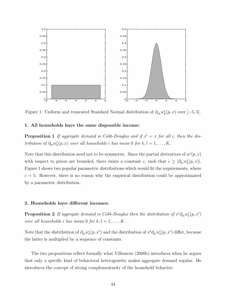
Figure 1: Uniform and truncated Standard Normal distribution of ∂pkwi
k(p, x) over [−5, 5].
1. All households have the same disposable income:
Proposition 1 If aggregate demand is Cobb-Douglas and if xi = x for all i, then the dis-
tribution of ∂plwi
k(p, x) over all households i has mean 0 for k, l = 1, . . . , K.
Note that this distribution need not to be symmetric. Since the partial derivatives of wi(p, x)
with respect to prices are bounded, there exists a constant c, such that c ≥ |∂plwi
k(p, x)|.Figure 1 shows two popular parametric distributions which would fit the requirements, where
c = 5. However, there is no reason why the empirical distribution could be approximated
by a parametric distribution.
2. Households have different incomes:
Proposition 2 If aggregate demand is Cobb-Douglas then the distribution of xi∂plwi
k(p, xi)
over all households i has mean 0 for k, l = 1, . . . , K.
Note that the distribution of ∂plwi
k(p, xi) and the distribution of xi∂pl
wik(p, x
i) differ, because
the latter is multiplied by a sequence of constants.
The two propositions reflect formally what Villemeur (2000b) introduces when he argues
that only a specific kind of behavioral heterogeneity makes aggregate demand regular. He
introduces the concept of strong complementarity of the household behavior:
44

0 10 20 30 40 50 60 70 80 90 100−500
−400
−300
−200
−100
0
100
200
300
400
500
x ∂
pk
wk(p
,x)
x
Figure 2: Illustration of a possible joint distribution of x and x∂pkwk(p, x). The marginal
distributions of ∂pkwk(p, x) and x∂pk
wk(p, x) are different.
Definition 1 (Villemeur 2000b) The households (wi, xi)i=1,...,n are said to display strong
behavioral complementarities if their aggregate expenditure share is constant in prices, i.e.
W (p) = c.
Strong complimentary household behavior smoothes the aggregate expenditure share to a
constant. Indeed, the conditions for strong behavioral complementarity are given in Propo-
sition 1 and Proposition 2.
An interesting fact can be inferred from Proposition 2. It is easy to see that the forces
which make the Law of demand hold are driven not only by the composition of the household
expenditure shares within the economy, but also by the shape of the income distribution.
We therefore have to consider the joint empirical distribution of the income xi and the
partial derivatives of wik(p, x
i) with respect to prices. Figure 2 shows the joint distribution
for a population of 1000 households. The marginal distribution of ∂pkwk(p, x) is the uniform
distribution over [−5, 5] and the household incomes are log normally distributed. The shaded
area illustrates the support of the joint distribution.
General Case Let us now consider the general case when W (p) is a function of prices.
We obtained some conditions in Lemma 2 that we are now reformulating in order to obtain
some more convenient expressions. This convenience will be mainly based on the fact that
we approximate empirical distributions by continuous distribution functions. We state two
45
additional assumptions:
Assumption 3 The empirical income distribution Gn(x) = n−1∑
i 1Ixi≤x converges uni-
formly to a continuous cumulative distribution function G(x) with density gx(x) and mean
value µ as n becomes large.
This assumption has several implications. Firstly, the uniform convergence allows us to sub-
stitute empirical frequencies by nicely behaved distribution functions. Secondly, continuity
of the distribution is required for technical purposes. Moreover, it is precluded that there is
one single household that dominates the whole economy in terms of disposable income.
Assumption 4 The economy is large, i.e. n is large, such that supx|Gn(x)−G(x)| < ε for
any ε > 0.
Let us now define some functions which assign values to the diagonal elements of the Jacobian
of household demand with respect to prices.
Definition 2 Let aik(p, x
i) := pk∂pkwi
k(p, xi) − wi
k(p, xi) be the diagonal value function for
household i and let ak,n(p, x) :=∑n
i=1 1Ixi=xaik(p, x
i) be the population diagonal value function
at a given level of income x, where 1I denotes the indicator function.
In addition, we use accordingly a definition for the off-diagonal elements:
Definition 3 Let bikl(p, x
i) := pk∂plwi
k(p, xi) be the off-diagonal value function of household
i and bkl,n(p, x) =∑n
i=1 1Ixi=xpk∂plwi
k(p, xi) the population off-diagonal value function at a
given level of income x.
Let us now state two assumptions on the functions defined above, which can be considered
as smoothness conditions across the income levels for a sufficiently large economy.
Assumption 5 ak,n(p, x) converges uniformly to a finite function ak(p, x) that is continuous
in p and x for all k.
Assumption 6 bkl,n(p, x) converges uniformly to a finite function bkl(p, x) that is continuous
in p and x for all k, l.
Assumptions 5 and 6 can be justified by a law of large numbers. As already mentioned in the
previous paragraph, the shape of the functions ak and bkl is driven by two impacts: first, aik
and bikl reflect the behavior of households and second, the sum over the indicator functions is
an empirical frequency and therefore connected to the empirical income distribution. Using
assumptions 3 and 4 we obtain a very useful separation for these two impacts:
46
Lemma 3 The influence of household behavior and the income distribution on the structure
of aggregate demand can be separated:
ak(p, x) = nak(p, x)gx(x),
where
ak(p, x) = limn→∞ak,n(p, x)∑
i 1Ixi=x
.
Define ak(p, x) = 0 whenever gx(x) = 0. Note that ak(p, x) is continuous in p and x due to
assumptions 3, 4 and 5. The same separation can be used for bkl(p, x). The question now
arises, what is the exact meaning of ak and bkl? Suppose there are j = 1, . . . , nj households
with income xj = x. Then
ak(p, x) = limn→∞
∑i 1Ixi=x (∂pk
wik(p, x)− wi
k(p, x))∑i 1Ixi=x
= limn→∞
∑nj
j=1
(∂pk
wjk(p, x)− wj
k(p, x))
nj
and an accordingly defined bkl(p, x) is the mean behavior of households with income x at
prices p. Assumptions 3,4,5 and 6 imply that these two functions vary smoothly with changes
in prices and across the income levels.
Let us now use the above results to define functions which determine the values of the
diagonal and off-diagonal elements for the Jacobian of aggregate demand with respect to
prices:
Definition 4 Let
Ak(p) :=
∫
IR+
x
Xak(p, x)dx
= n
∫
IR+
x
Xak(p, x)gx(x)dx
be the aggregate diagonal value function for k = 1, . . . , K.
Definition 5 Let
Bkl(p) :=
∫
IR+
x
Xbkl(p, x)dx
= n
∫
IR+
x
Xbkl(p, x)gx(x)dx for k, l = 1, . . . , K
be the aggregate off-diagonal value function.
47
We can now formulate the main result of this section:
Proposition 3 Under assumptions 1-6 the Law of demand for aggregate demand of a het-
erogenous population (f i, xi)i=1,...,n holds if Ak(p) and Bkl(p) satisfy
Ak(p) < 0 for k = 1, . . . , K
and
|Ak(p)| ≥∑
l 6=k
|Bkl(p)| for k = 1, . . . , K.
Proof. The first condition ensures negative diagonal elements of the Jacobian matrix of
aggregate demand as they are given in Lemma 2. The second condition can be rewritten as
∫
R+
[|ak(p, x)| −
∑
l 6=k
∣∣∣bkl(p, x)∣∣∣]
gx(x)dx ≤ 0 for k = 1, . . . , K,
which is equivalent to the off-diagonal condition of Lemma 2. ¥
According to the definition of strong behavioral complementarity, Villemeur (2000b) also
considers the general case:
Definition 6 (Villemeur 2000b) The households (wi, xi)i=1,...,n are said to display behavioral
complementarities if the aggregate expenditure share W (p) verifies the Law of demand.
Proposition 3 presents the conditions for behavioral complementarity.
The following example might help in illustrating how the forces work which make the
Law of demand for aggregate demand hold.
Example 1 Suppose there are i = 1, . . . , n households and two commodities, i.e. K = 2.
From Proposition 3 we know that the Law of demand holds if the following inequalities are
true:∫
IR+
nx
Xak(p, x)gx(x)dx < 0 and
∣∣∣∣∫
IR+
nx
Xak(p, x)gx(x)dx
∣∣∣∣ ≥∣∣∣∣∫
IR+
nx
Xbkl(p, x)gx(x)dx
∣∣∣∣ for k, l = 1, 2, k 6= l
Using integration by parts, the first inequality can be rewritten as:
µak(p,∞) <
∫
IR+
[∫ x
0
1−G(τ)dτ
]∂xak(p, x)dx,
48

0 20 40 600
0.01
0.02
0.03
0.04
0.05
0.06
0.07
0.08
0.09
x
gx(x,γ,σ2)
0 20 40 600
2
4
6
8
10
12
14
x
G(x,γ+σ2,σ2)*exp(γ+0.5*σ2)
Figure 3: Logarithmic normal distribution of x with γ = 2.2 and σ2 = 0.7 (left); correspond-
ing incomplete moment function (right).
where again integration by parts yields∫IR+
1 − G(x)dx = µ, the mean household income.
The left hand side is a constant and the right hand side contains the incomplete first moment
function of the underlying income distribution. The second inequality holds if∣∣∣∣µak(p,∞)−
∫
IR+
[∫ x
0
1−G(τ)dτ
]∂xak(p, x)dx
∣∣∣∣
≥∣∣∣∣µbkl(p,∞)−
∫
IR+
[∫ x
0
1−G(τ)dτ
]∂xbkl(p, x)dx
∣∣∣∣ ,
where µak(p,∞) and µbkl(p,∞) are equal to 0, since limx→∞gx(x) = 0 induces limx→∞ak(p, x) =
bkl(p, x) = 0 for all k 6= l.
Suppose in addition that the empirical income distribution can be approximated by a
logarithmic normal distribution with parameters γ and σ2. Note that in this case µ =exp{γ+
0.5σ2} and following Butler and McDonald (1989) one can show that
∫ x
0
(1−G(τ ; γ, σ2)
)dτ = µG(x; γ + σ2, σ2)
holds. Figure 3 plots the density of the income distribution for empirically evident parameter
values σ and µ, and the corresponding incomplete first moment function. The incomplete
first moment function is positive and nondecreasing from 0 to µ and can be interpreted as
a weight function that assigns low weights to relatively poor households and large weights to
relatively rich households. Therefore, the behavior of richer households is weighted at least
49

as much as that of poorer households. From Figure 3 it is apparent that for a large fraction
of the population the incomplete first moment function is close to zero. For a given level of
income x = 8.5, we obtain G(8.5, 2.2, 0.7) = 0.47 and G(8.5, 2.9, 0.7)exp{2.55} = 1.77. This
means that to almost 50% of the population has been assigned a weight less than or equal to
1.8. To see this look at the shaded areas in Figure 1. The richest households are assigned
a weight up to a value of 12. Note that ∂xak(p, x) and ∂xbkl(p, x) converge to 0 for x large
enough (> 60) since gx(x) approaches 0. For x small enough we cannot infer mathematical
properties for ∂xak and ∂xbkl(p, x) from the above assumptions. Nevertheless, one might ask
whether the partial derivatives are larger for low incomes in order to have some counter effect
to the low income weights for poorer households. Intuitively, there is no reason for this to
happen since we are considering the mean behavior of households with the same income.
This example deepens the analysis of how both the aggregated demand behavior, ex-
pressed by the functions ak and bk, and the shape of the income distribution are the main
determinants of the structure of aggregate demand. Moreover, it turns out that the behavior
of poorer households plays a less important role than the one of richer households. This is
in accordance with what we already found out discussing Propositions 1 and 2. Note that
this effect is due to the fact that we are using expenditure shares as opposed to demand
functions. If the latter were used this effect would be ruled out since demand is measured
in absolute values.
This section has demonstrated that a somewhat heterogenous population may have an
aggregate demand function for which the Law of demand holds. Propositions 1-3 show the
conditions required for the distribution of household heterogeneity. Nevertheless, it it is not
yet clear, whether heterogeneity in general or just a specific kind of heterogeneity causes
the Law of demand to hold. The purpose of the following sections is to present existing
definitions of behavioral heterogeneity and to introduce a new one.
50

3 Behavioral Heterogeneity: Definitions and Impacts
Considering the recent literature, behavioral heterogeneity has been defined in various ways.
The contributions of Grandmont (1992), Kneip (1999) and Hildenbrand and Kneip (1999)
are all concerned with the same topic but each use different concepts. Since the definition
of behavioral heterogeneity is essential for further analysis we engage this problem in this
section. After a review of existing definitions, a new definition is introduced. Moreover the
impacts of behavioral heterogeneity on the shape of aggregate demand are presented using
the framework of the previous section.
Something upon which all scientists may agree is that in the case of extreme behavioral
homogeneity all households possess the same demand function. Finding a commonly ac-
cepted definition of behavioral heterogeneity is more difficult. The definition of behavioral
heterogeneity is widely based on the dispersion of household characteristics. Grandmont
(1992), Kneip (1999) and Hildenbrand and Kneip (1999) use this concept in order to show
that if the households behaved extremely heterogeneously, the Law of demand for aggre-
gate demand holds, even if none of the households behaves accordingly. The reasoning for
using the dispersion of characteristics for measuring behavioral heterogeneity is explained
for example by Villemeur (2000b): increasing dispersion of household characteristics means
that we have less a priori information about the type of a household which is randomly
chosen from the population. In other words low entropy means behavioral heterogeneity.
As pointed out by Villemeur, this concept makes sense when considering compact spaces
of parameters that differ across the households and which have some influence on the de-
mand behavior of the households. If the space of parameters was not bounded, and even
not observable, the reasoning becomes more complicated since the formulation can easily
become an artificial construction. Intuitively, one can also refer to the dispersion over the
space of feasible behavior. This definition is also based on the distribution on the parameter
spaces of demand or even in the space of feasible expenditure shares. Figure 4 illustrates
both concepts: on the top we see a distribution in the space of admissible demand functions
W . Extreme behavioral heterogeneity corresponds in this case to all subsets of W having
same probability. More specifically, in the middle we see a distribution of parameters α. If
all households had the same demand function and only differ in this parameter, one can say
that the flatter the distribution of α the more heterogeneously the population behaves.
Alternatively, one might also use the distance of the images of household expenditure
51
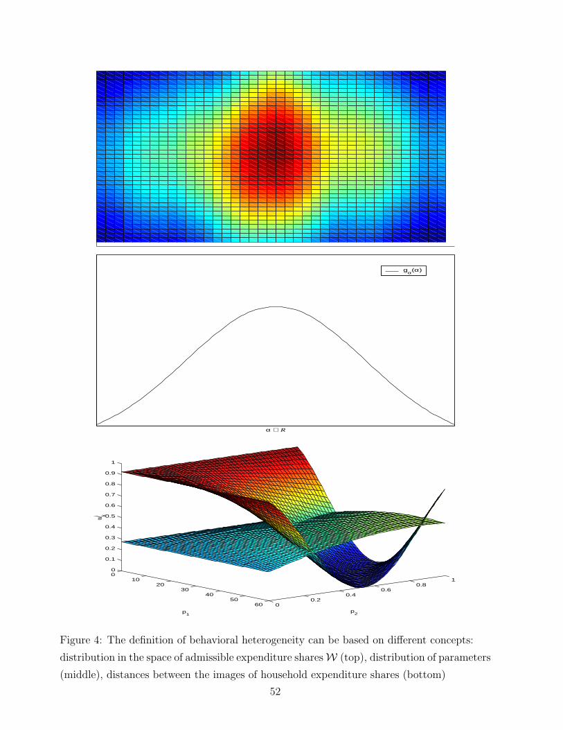
α ∈ R
gα(α)
010
2030
4050
60 00.2
0.40.6
0.81
0
0.1
0.2
0.3
0.4
0.5
0.6
0.7
0.8
0.9
1
p2p
1
wi k
Figure 4: The definition of behavioral heterogeneity can be based on different concepts:
distribution in the space of admissible expenditure sharesW (top), distribution of parameters
(middle), distances between the images of household expenditure shares (bottom)
52
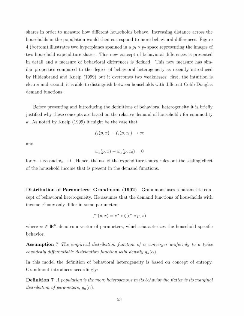
shares in order to measure how different households behave. Increasing distance across the
households in the population would then correspond to more behavioral differences. Figure
4 (bottom) illustrates two hyperplanes spanned in a p1×p2 space representing the images of
two household expenditure shares. This new concept of behavioral differences is presented
in detail and a measure of behavioral differences is defined. This new measure has sim-
ilar properties compared to the degree of behavioral heterogeneity as recently introduced
by Hildenbrand and Kneip (1999) but it overcomes two weaknesses: first, the intuition is
clearer and second, it is able to distinguish between households with different Cobb-Douglas
demand functions.
Before presenting and introducing the definitions of behavioral heterogeneity it is briefly
justified why these concepts are based on the relative demand of household i for commodity
k. As noted by Kneip (1999) it might be the case that
fk(p, x)− fk(p, x0) →∞
and
wk(p, x)− wk(p, x0) = 0
for x →∞ and x0 → 0. Hence, the use of the expenditure shares rules out the scaling effect
of the household income that is present in the demand functions.
Distribution of Parameters: Grandmont (1992) Grandmont uses a parametric con-
cept of behavioral heterogeneity. He assumes that the demand functions of households with
income xi = x only differ in some parameters:
fα(p, x) = eα ∗ ζ(eα ∗ p, x)
where α ∈ IRK denotes a vector of parameters, which characterizes the household specific
behavior.
Assumption 7 The empirical distribution function of α converges uniformly to a twice
boundedly differentiable distribution function with density gα(α).
In this model the definition of behavioral heterogeneity is based on concept of entropy.
Grandmont introduces accordingly:
Definition 7 A population is the more heterogenous in its behavior the flatter is its marginal
distribution of parameters, gα(α).
53
Heterogeneity is measured by the flatness of the distribution of α:∫
IR|∂αk
gα(α)|.
Assumption 8 fα(p, x) is homogeneous of degree 0 in p and x.
Assumption 9 fα(p, x) satisfies Walras’s law, i.e. p ∗ fα(p, x) = x.
Assumption 10 Aggregate demand F (p) is bounded from below for p ∈ IRK : ∃c ∈ IRK++,
such that F (p) ≥ c.
Under these assumptions Grandmont proves the following proposition:
Proposition 4 (Grandmont 1992) Extreme behavioral heterogeneity, i.e. supk
∫IR|∂αk
gα(α)|dα =
0, causes the Law of demand to hold for aggregate demand.
The proof follows from the fact that he shows:∣∣∣∣∫
IRK
∂plwk(e
α ∗ p, x)gα(α)dα
∣∣∣∣ ≤supp,x|wk(e
α ∗ p, x)|pl
(∫
IRK
|∂αlgα(α)|dα
)(5)
for all k, l. Using Lemma 2, extreme behavioral heterogeneity in this model therefore induces
the off-diagonal elements of the Jacobian of aggregate demand to be zero. The first term of
he diagonal elements also vanishes and the remaining second term is strictly positive due to
assumption 10. The Jacobian of aggregate demand is therefore negative diagonal dominant,
having a negative real part of its largest characteristic value.
Villemeur (1998) shows that household demand in this setting becomes more insensitive
with respect to price changes the larger is |αk|. He also points out that an extremely flat
distribution, i.e. a uniform distribution, of α on IRK implies that the mass of a compact set
on the support of α converges to 0. Therefore, the mass of this distributions is allocated to
asymptotically large values of α. In this case most of the households in this model are insen-
sitive, i.e. Cobb-Douglas-like, to price changes. Extreme behavioral heterogeneity therefore
corresponds to having a population consisting of Cobb-Douglas like behaving households.
Distribution of behavior: Kneip (1999) In contrast to the former approach, Kneip
considers the distribution of a continuum of functions w ∈ W , where W is the space of
admissible expenditure shares. He defines a probabilistic framework resulting in a well de-
fined probability measure ν on the smallest σ-Algebra of the space of admissible expenditure
shares W . Details of this measure theory based approach are not presented here. Based on
the model introduced in Section 2 we consider an economy with a discrete set of households.
54

Kneip analyzes aggregate demand conditional on a given level of income x:
F (p, x) = xp−1 ∗nj∑
j=1
wj(p, x)
He proves weak sensitivity of the sum, i.e. it has a small partial derivative with respect to a
price, induces structure and definiteness on the Jacobian of aggregate demand. In order to
measure the sensitivity of the above sum, Kneip introduces:
Definition 8 Let ν denote the empirical distribution of wi ∈ W. The coefficient of sensi-
tivity
h(ν) := maxk,l{supp,x|∂pl
nj∑j=1
wjk(p, x)|}
measures the sensitivity of the aggregate expenditure share to price changes.
Definition 9 Aggregate demand is defined as structurally stable whenever the coefficient of
sensitivity is small enough.
It is shown that structural stability of aggregate demand is caused by invariability of the
household expenditure shares with respect to prices changes, meaning that all households
behave as if Cobb-Douglas. Moreover, Kneip postulated that structural stability is also
caused by extreme behavioral heterogeneity, where he defines the latter as:
Definition 10 Extreme behavioral heterogeneity of a population is equivalent to all subsets
of W of a given and equal size having the same probability.
This concept intuitively corresponds to ’pointwise’ heterogeneity. Each feasible behavior oc-
curs with the same probability. This can be formalized as follows: Given a subset J ∈ [0, 1]K ,
the image space of admissible expenditure shares, we have a high amount of heterogeneity
if for all J
ν{wi ∈ W|w(p, x) ∈ J
} ≈ ν{wi ∈ W|w(q, y) ∈ J
}
holds, where q and y are transformed p and x.
Kneip shows under assumptions 1-3 and 10:
Proposition 5 (Kneip 1999) Structural stability induces a negative definite Jacobian of
aggregate demand.
55
The proof in our framework follows immediately from Lemma 2 with the same reasoning as in
the Grandmont model. Clearly these conditions are stronger than required since the weight-
ing of income is not considered since F (p, x) has a negative dominant diagonal for all given
x. This means in particular that the functions bkl(p, x) are close to zero and ak(p, x) < 0 for
all k, l, p and x.
It is not very easy to construct an example which intuitively points out the meaning of
’pointwise’ heterogeneity since its definition is quite abstract. It is difficult to imagine the
impact of a uniform distribution over the space of feasible expenditure shares.
Example 2 Consider an economy in which all households have the same income xi = x.
Suppose for instance that extreme behavioral heterogeneity as defined above induces a uniform
distribution of wik(p, x) on [0, 1] for k = 1, 2 and all p ∈ [0, 1]K. Then, for all k, Wk(p) =∑n
i=1 wik(p, x) converges uniformly in p to 0.5 as n becomes large. Aggregate demand is
therefore Cobb-Douglas with∑2
k=1 Wk(p) = 1. More generally, define pk = (p1, . . . , pk−1, ∆+
pk, pk+1, . . . , pK), where ∆ ∈ IR+. Then
n∑i=1
wik(p, x
i) =n∑
i=1
wik(pl, x) for k, l = 1, . . . , K
follows. Therefore, by Proposition 1 the Law of demand for aggregate demand holds since
0 = lim∆→0∆pk
n∑i=1
wik(pl, x)− wi
k(p, x)
∆
= ∆pk
n∑i=1
∂plwi
k(p, x) for k, l = 1, . . . , K
and xi = x for all i. The same reasoning holds if the empirical distribution of wik(p, x
i) on
[0, 1] is a uniform distribution independent of the prices and the income. This example can
be considered to be related to Becker’s (1962) pioneering findings. He shows that if a uniform
distribution of wik(p, x) on the budget line is not affected by price changes, then aggregate
demand is declining.
Kneip’s approach has been subject to criticism. Villemeur (1999) argues that a uniform
distribution over an infinite ’space of behavior’ gives all the weight to its boundary elements.
He concludes that behavioral heterogeneity in this setup ’reduces dramatically the set of
admissible expenditure share functions ’, whereby it does not necessarily follow that this set
only consists of Cobb-Douglas like households as in the Grandmont model. Maret (2001)
56

and Giraud and Maret (2001) show that Kneip’s result can also be achieved when W is
a compact set. In this case the mass of the distribution is not allocated on the boundary
and therefore it is not anymore subject to Villemeur’s criticism. Moreover, they show that
extreme behavioral heterogeneity corresponds to strong behavioral heterogeneity as given in
Definition 1.
Distribution of partial derivatives: Hildenbrand and Kneip (1999) Hildenbrand
and Kneip introduce an index, γ ∈ [0, 1), that measures the degree of behavioral hetero-
geneity of the population. They show under assumptions 1-3 that the Law of demand
for aggregate Demand holds if the demand behavior of the population is sufficiently het-
erogenous. Roughly speaking, their definition of behavioral heterogeneity is based on the
distribution of the partial derivatives of household expenditure shares with respect to prices.
For λ > 0 define
Skl(p) := ∂λWk(p1, . . . , λpl, . . . , pK)|λ=1 = pl∂plWk(p)
as the rate of change of Wk(p) with respect to a percentage change of the price pl. Accordingly
one obtains for each household
sikl(p, x
i) := ∂λwik(p1, . . . , λpl, . . . , pK , xi)|λ=1 = pl∂pl
wik(p, x
i).
Moreover, the upper bound for |sikl(p, x
i)| with respect to prices is given by
dikl := supp|si
kl(p, xi)| = supppl|∂pl
wik(p, x
i)|.
Let δ ∈ [0, 1]. The domain of prices in which pl|∂plwi
k(p, xi)| ≥ δdi
kl is defined as
Aδkl(w
i, xi) := {p ∈ (0,∞)K | pl|∂plwi
k(p, xi)| ≥ δdi
kl}.
In order to define the measure for the degree of behavioral heterogeneity of a population, it
is important to clarify what Hildenbrand and Kneip (1999) mean by behavioral heterogeneity:
Aδkl(w
i, xi) are located in different regions of the price system in (0,∞)K across the households
i. Accordingly, they define an intersection ratio
Iδkl(p) :=
1
ncard{i|p ∈ Aδ
kl(wi, xi)}
which indicates by how much the sets Aδkl(w
i, xi) differ across the households i. Note that
Iδkl(p) is a decreasing step function in δ. A high degree of behavioral heterogeneity implies
a low intersection ratio. Then∫ 1
0Iδkl(p)dδ is close to zero. Taking this into account, let us
now define the degree of behavioral heterogeneity of the household population:
57

Definition 11 The degree of behaviorial heterogeneity of a population is measured by the
index of heterogeneity γ, where
γ := infk,l,pγkl(p) = 1− supk,l,p
∫ 1
0
Iδkl(p)dδ.
Note that 0 ≤ γ ≤ 1− 1n
< 1.
Hildenbrand and Kneip (1999) show that a sufficiently small index of heterogeneity im-
plies the Law of demand for mean demand, although this property was not assumed for
household demands:
Proposition 6 A sufficiently high degree of behavioral heterogeneity implies negative diag-
onal dominance of the Jacobian matrix of mean demand with respect to prices if there is a
constant c ≥ 0 such that dikl ≤ c for all k, l, i.
Villemeur (2000a) has shown that in the Hildenbrand and Kneip framework, extreme
behavioral heterogeneity corresponds to a population of households that are mostly insensi-
tive to price changes but in which for each household i, there exists a small area of prices at
which i’s demand is sensitive to price changes. Their definition of behavioral heterogeneity
induces γ = 0 if all households have the same or a Cobb-Douglas demand function. Clearly,
in this case there is no heterogeneity in the distribution of the partial derivatives across the
households. Their example of extreme behavioral heterogeneity is the Grandmont economy
with a flat distribution of α. As already noted, in this case the main part of the population
behaves Cobb-Douglas-like for given prices.
Behavioral differences In what follows, the concept of behavioral heterogeneity is based
on the distance of the images of household expenditure shares. In contrast to the framework
defined in Section 2 the price system is now normalized to [0, 1]K . The distance between the
expenditure shares with given income xi = x is measured on its support, which is the price
system. For this purpose we use the Euclidian distance:
Definition 12 The Euclidian distance between the images of the functions wik(p, x) and
wjk(p, x) is defined as
‖wik(p|x)− wj
k(p|x)‖2 :=
[∫
(0,1]K
(wi
k(p, x)− wjk(p, x)
)2dp
]1/2
.
58
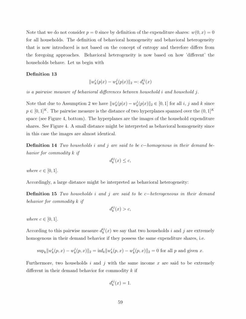
Note that we do not consider p = 0 since by definition of the expenditure shares: w(0, x) = 0
for all households. The definition of behavioral homogeneity and behavioral heterogeneity
that is now introduced is not based on the concept of entropy and therefore differs from
the foregoing approaches. Behavioral heterogeneity is now based on how ’different’ the
households behave. Let us begin with
Definition 13
‖wik(p|x)− wj
k(p|x)‖2 =: dijk (x)
is a pairwise measure of behavioral differences between household i and household j.
Note that due to Assumption 2 we have ‖wik(p|x)−wj
k(p|x)‖2 ∈ [0, 1] for all i, j and k since
p ∈ [0, 1]K . The pairwise measure is the distance of two hyperplanes spanned over the (0, 1]K
space (see Figure 4, bottom). The hyperplanes are the images of the household expenditure
shares. See Figure 4. A small distance might be interpreted as behavioral homogeneity since
in this case the images are almost identical.
Definition 14 Two households i and j are said to be c−homogenous in their demand be-
havior for commodity k if
dijk (x) ≤ c,
where c ∈ [0, 1].
Accordingly, a large distance might be interpreted as behavioral heterogeneity:
Definition 15 Two households i and j are said to be c−heterogeneous in their demand
behavior for commodity k if
dijk (x) > c,
where c ∈ [0, 1].
According to this pairwise measure dijk (x) we say that two households i and j are extremely
homogenous in their demand behavior if they possess the same expenditure shares, i.e.
supk‖wik(p, x)− wj
k(p, x)‖2 = infk‖wik(p, x)− wj
k(p, x)‖2 = 0 for all p and given x.
Furthermore, two households i and j with the same income x are said to be extremely
different in their demand behavior for commodity k if
dijk (x) = 1.
59
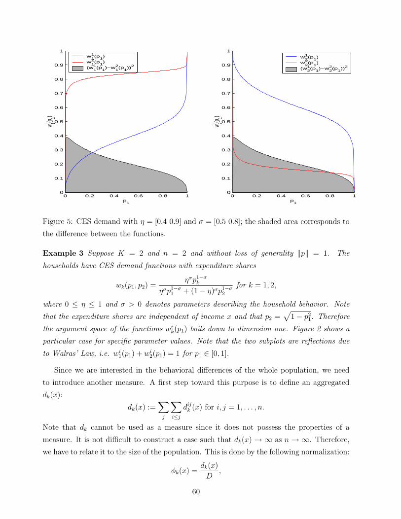
0 0.2 0.4 0.6 0.8 10
0.1
0.2
0.3
0.4
0.5
0.6
0.7
0.8
0.9
1
p1
wi 1(p 1)w1
1(p
1)
w21(p
1)
(w11(p
1)−w2
1(p
1))2
0 0.2 0.4 0.6 0.8 10
0.1
0.2
0.3
0.4
0.5
0.6
0.7
0.8
0.9
1
p1
wi 2(p 1)
w12(p
1)
w22(p
1)
(w12(p
1)−w2
2(p
1))2
Figure 5: CES demand with η = [0.4 0.9] and σ = [0.5 0.8]; the shaded area corresponds to
the difference between the functions.
Example 3 Suppose K = 2 and n = 2 and without loss of generality ‖p‖ = 1. The
households have CES demand functions with expenditure shares
wk(p1, p2) =ησp1−σ
k
ησp1−σ1 + (1− η)σp1−σ
2
for k = 1, 2,
where 0 ≤ η ≤ 1 and σ > 0 denotes parameters describing the household behavior. Note
that the expenditure shares are independent of income x and that p2 =√
1− p21. Therefore
the argument space of the functions wik(p1) boils down to dimension one. Figure 2 shows a
particular case for specific parameter values. Note that the two subplots are reflections due
to Walras’ Law, i.e. wi1(p1) + wi
2(p1) = 1 for p1 ∈ [0, 1].
Since we are interested in the behavioral differences of the whole population, we need
to introduce another measure. A first step toward this purpose is to define an aggregated
dk(x):
dk(x) :=∑
j
∑i≤j
dijk (x) for i, j = 1, . . . , n.
Note that dk cannot be used as a measure since it does not possess the properties of a
measure. It is not difficult to construct a case such that dk(x) →∞ as n →∞. Therefore,
we have to relate it to the size of the population. This is done by the following normalization:
φk(x) =dk(x)
D,
60
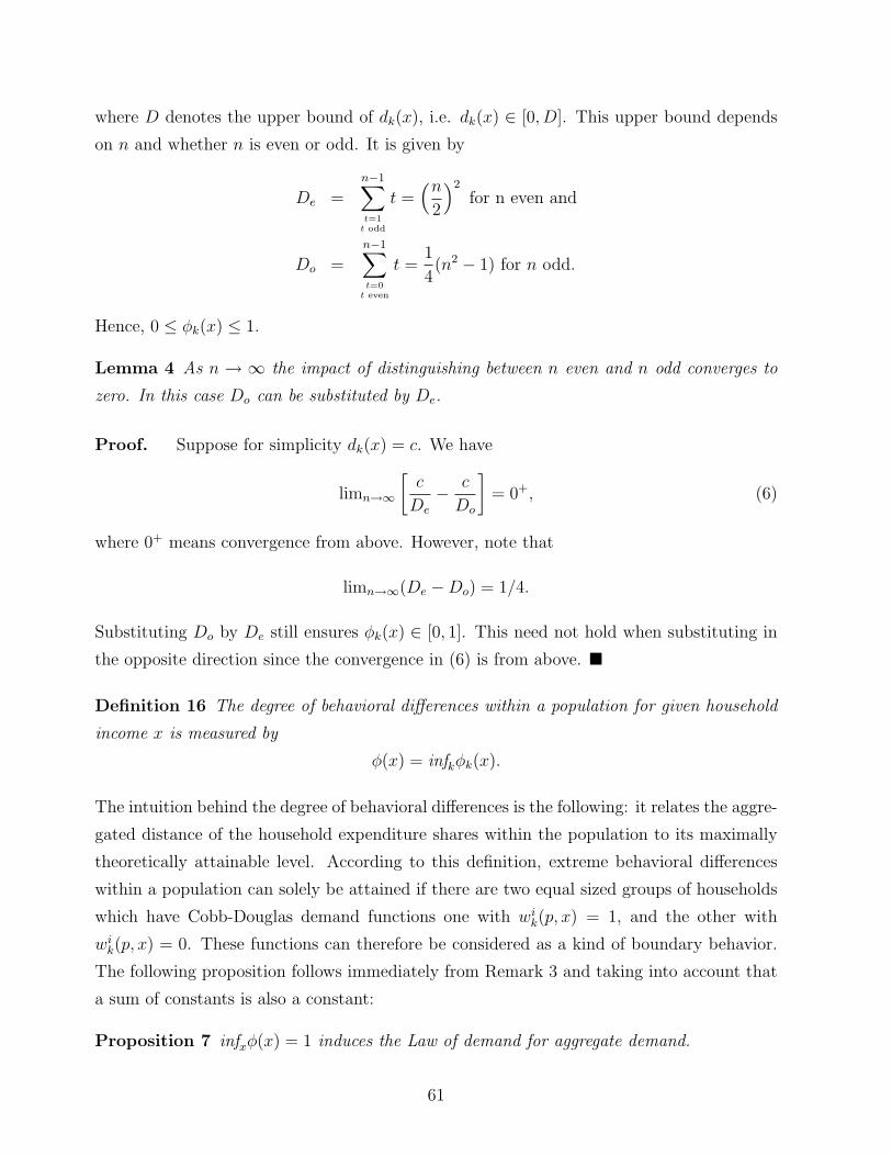
where D denotes the upper bound of dk(x), i.e. dk(x) ∈ [0, D]. This upper bound depends
on n and whether n is even or odd. It is given by
De =n−1∑t=1
t odd
t =(n
2
)2
for n even and
Do =n−1∑t=0
t even
t =1
4(n2 − 1) for n odd.
Hence, 0 ≤ φk(x) ≤ 1.
Lemma 4 As n → ∞ the impact of distinguishing between n even and n odd converges to
zero. In this case Do can be substituted by De.
Proof. Suppose for simplicity dk(x) = c. We have
limn→∞
[c
De
− c
Do
]= 0+, (6)
where 0+ means convergence from above. However, note that
limn→∞(De −Do) = 1/4.
Substituting Do by De still ensures φk(x) ∈ [0, 1]. This need not hold when substituting in
the opposite direction since the convergence in (6) is from above. ¥
Definition 16 The degree of behavioral differences within a population for given household
income x is measured by
φ(x) = infkφk(x).
The intuition behind the degree of behavioral differences is the following: it relates the aggre-
gated distance of the household expenditure shares within the population to its maximally
theoretically attainable level. According to this definition, extreme behavioral differences
within a population can solely be attained if there are two equal sized groups of households
which have Cobb-Douglas demand functions one with wik(p, x) = 1, and the other with
wik(p, x) = 0. These functions can therefore be considered as a kind of boundary behavior.
The following proposition follows immediately from Remark 3 and taking into account that
a sum of constants is also a constant:
Proposition 7 infxφ(x) = 1 induces the Law of demand for aggregate demand.
61

Extreme behav-
ioral heterogeneity
Households posses the
same demand function
Households posses Cobb-
Douglas demand
value of the index
Coefficient of sensi-
tivity
0 0 ≤ h < ∞ 0
Degree of behavioral
heterogeneity
1 0 0
Degree of behavioral
differences
1 0 0 ≤ φ ≤ 1
Table 1: Comparison of the different concepts for the modelling of behavioral heterogeneity.
Note that there is no index in the Grandmont approach.
A maximal φ(x) for all x corresponds to a population of Cobb-Douglas households. This
property is obviously stronger than required. In order to make the Law of demand for ag-
gregate demand hold it should therefore be sufficient to have a high degree of behavioral
differences. However, differences in the Cobb-Douglas demand functions across the house-
holds now matter. This is in contrast to the approaches of Kneip (1999) and Hildenbrand
and Kneip (1999). Meaning that the degree of behavioral differences can still be between
zero and one whenever all households possess Cobb-Douglas demand functions. It is only
zero if all households with the same income x possess the same expenditure share for at least
one commodity k.
Let us conclude this section by briefly summarizing the main properties of the foregoing
indices which result from different modelling concepts. Table 1 provides an overview. The
coefficient of sensitivity does not distinguish between extreme behavioral heterogeneity and
the case when all households have the same Cobb-Douglas demand function. The degree
of behavioral heterogeneity overcomes this weakness and is bounded. However, it is always
zero if the households posses Cobb-Douglas demand functions even with different param-
eters. This is in contrast to the degree of behavioral differences which is only zero if all
households have the same demand function for at least one good given an income.
For future research it might be interesting to consider the following1: Suppose we have a
given distribution of households. Is it possible to derive thresholds for the indices, such that
1This point has been suggested by Wolfgang Leininger.
62
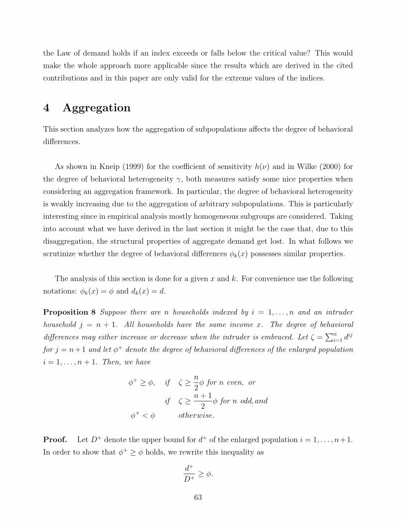
the Law of demand holds if an index exceeds or falls below the critical value? This would
make the whole approach more applicable since the results which are derived in the cited
contributions and in this paper are only valid for the extreme values of the indices.
4 Aggregation
This section analyzes how the aggregation of subpopulations affects the degree of behavioral
differences.
As shown in Kneip (1999) for the coefficient of sensitivity h(ν) and in Wilke (2000) for
the degree of behavioral heterogeneity γ, both measures satisfy some nice properties when
considering an aggregation framework. In particular, the degree of behavioral heterogeneity
is weakly increasing due to the aggregation of arbitrary subpopulations. This is particularly
interesting since in empirical analysis mostly homogeneous subgroups are considered. Taking
into account what we have derived in the last section it might be the case that, due to this
disaggregation, the structural properties of aggregate demand get lost. In what follows we
scrutinize whether the degree of behavioral differences φk(x) possesses similar properties.
The analysis of this section is done for a given x and k. For convenience use the following
notations: φk(x) = φ and dk(x) = d.
Proposition 8 Suppose there are n households indexed by i = 1, . . . , n and an intruder
household j = n + 1. All households have the same income x. The degree of behavioral
differences may either increase or decrease when the intruder is embraced. Let ζ =∑n
i=1 dij
for j = n+1 and let φ+ denote the degree of behavioral differences of the enlarged population
i = 1, . . . , n + 1. Then, we have
φ+ ≥ φ, if ζ ≥ n
2φ for n even, or
if ζ ≥ n + 1
2φ for n odd, and
φ+ < φ otherwise.
Proof. Let D+ denote the upper bound for d+ of the enlarged population i = 1, . . . , n+1.
In order to show that φ+ ≥ φ holds, we rewrite this inequality as
d+
D+≥ φ.
63
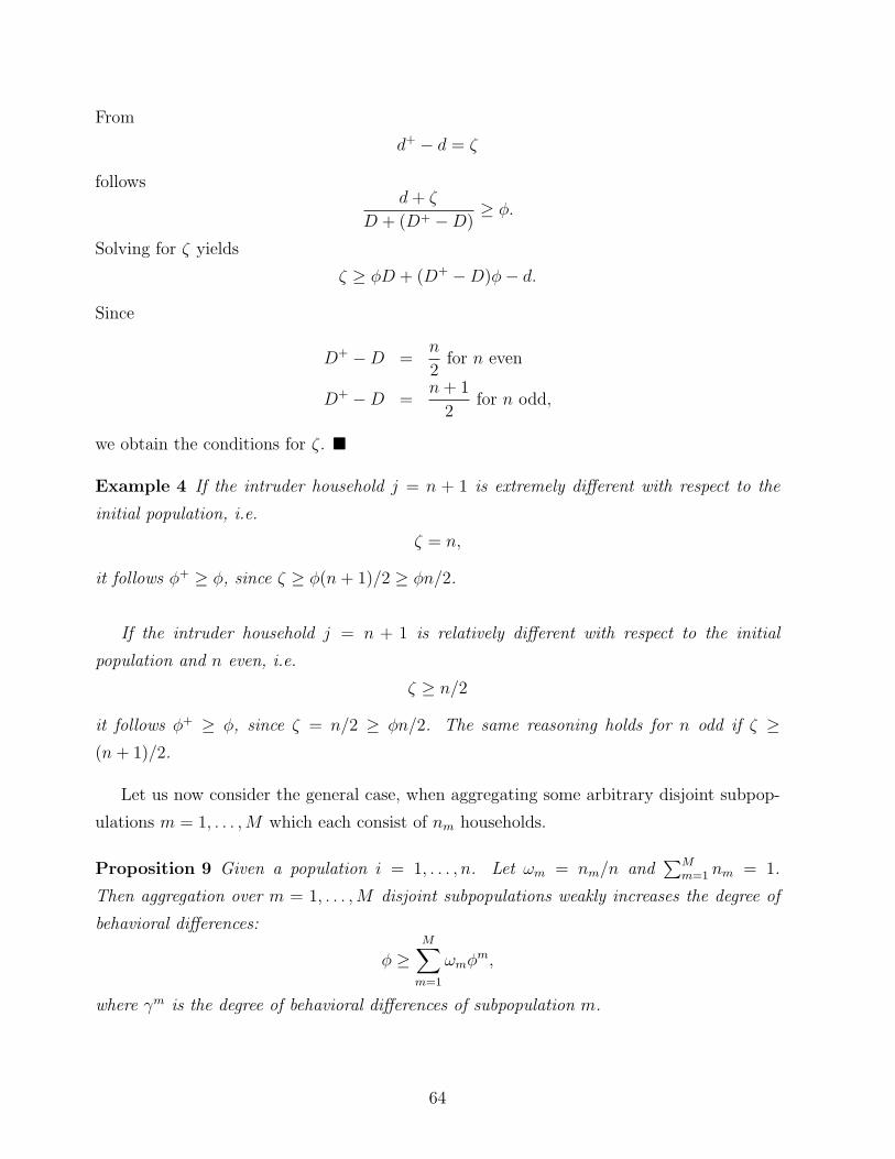
From
d+ − d = ζ
followsd + ζ
D + (D+ −D)≥ φ.
Solving for ζ yields
ζ ≥ φD + (D+ −D)φ− d.
Since
D+ −D =n
2for n even
D+ −D =n + 1
2for n odd,
we obtain the conditions for ζ. ¥
Example 4 If the intruder household j = n + 1 is extremely different with respect to the
initial population, i.e.
ζ = n,
it follows φ+ ≥ φ, since ζ ≥ φ(n + 1)/2 ≥ φn/2.
If the intruder household j = n + 1 is relatively different with respect to the initial
population and n even, i.e.
ζ ≥ n/2
it follows φ+ ≥ φ, since ζ = n/2 ≥ φn/2. The same reasoning holds for n odd if ζ ≥(n + 1)/2.
Let us now consider the general case, when aggregating some arbitrary disjoint subpop-
ulations m = 1, . . . , M which each consist of nm households.
Proposition 9 Given a population i = 1, . . . , n. Let ωm = nm/n and∑M
m=1 nm = 1.
Then aggregation over m = 1, . . . , M disjoint subpopulations weakly increases the degree of
behavioral differences:
φ ≥M∑
m=1
ωmφm,
where γm is the degree of behavioral differences of subpopulation m.
64
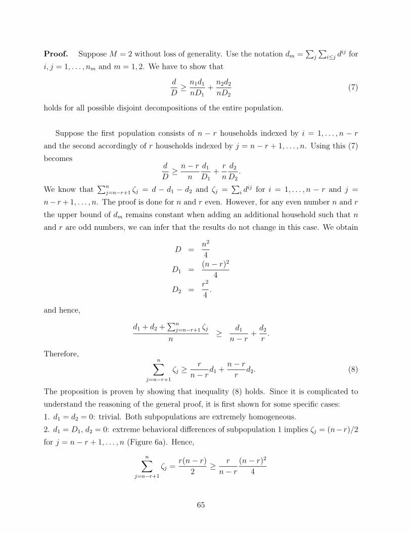
Proof. Suppose M = 2 without loss of generality. Use the notation dm =∑
j
∑i≤j dij for
i, j = 1, . . . , nm and m = 1, 2. We have to show that
d
D≥ n1d1
nD1
+n2d2
nD2
(7)
holds for all possible disjoint decompositions of the entire population.
Suppose the first population consists of n − r households indexed by i = 1, . . . , n − r
and the second accordingly of r households indexed by j = n− r + 1, . . . , n. Using this (7)
becomesd
D≥ n− r
n
d1
D1
+r
n
d2
D2
.
We know that∑n
j=n−r+1 ζj = d − d1 − d2 and ζj =∑
i dij for i = 1, . . . , n − r and j =
n− r + 1, . . . , n. The proof is done for n and r even. However, for any even number n and r
the upper bound of dm remains constant when adding an additional household such that n
and r are odd numbers, we can infer that the results do not change in this case. We obtain
D =n2
4
D1 =(n− r)2
4
D2 =r2
4.
and hence,
d1 + d2 +∑n
j=n−r+1 ζj
n≥ d1
n− r+
d2
r.
Therefore,n∑
j=n−r+1
ζj ≥ r
n− rd1 +
n− r
rd2. (8)
The proposition is proven by showing that inequality (8) holds. Since it is complicated to
understand the reasoning of the general proof, it is first shown for some specific cases:
1. d1 = d2 = 0: trivial. Both subpopulations are extremely homogeneous.
2. d1 = D1, d2 = 0: extreme behavioral differences of subpopulation 1 implies ζj = (n− r)/2
for j = n− r + 1, . . . , n (Figure 6a). Hence,
n∑j=n−r+1
ζj =r(n− r)
2≥ r
n− r
(n− r)2
4
65
0 0.1 0.2 0.3 0.4 0.5 0.6 0.7 0.8 0.9 1
0
0.2
0.4
0.6
0.8
1
p
w(p
)
Subpopulation 2: r*w2(p)
Subpopulation 1: 1*(n−r)/2
Subpopulation 1: 0*(n−r)/2
0 0.1 0.2 0.3 0.4 0.5 0.6 0.7 0.8 0.9 1
0
0.2
0.4
0.6
0.8
1
pw
(p)
Subpopulation 1: (n−r)*w1(p)
Subpopulation 2: 1*r/2
Subpopulation 2: 0*r/2
Figure 6: Illustration for∑
ζj = r(n−r)/2, if one of the subpopulations consists of extremely
differently behaving households; for simplicity: K = 1.
holds. Moreover, it holds for d2 ∈ [0, D2], whereby it is an equality for d2 = D2.
3. d1 = 0, d2 = D2: extreme behavioral differences of subpopulation 2 implies∑
ζj =
r(n− r)/2 (Figure 6b). Hence,
n∑j=n−r+1
ζj =r(n− r)
2≥ n− r
r
r2
4
holds. Moreover, it holds for d1 ∈ [0, D1], whereby it is an equality for d1 = D1.
General Case: d1 = D1 − δ1, d2 = D2 − δ2, where δ1 ∈ [0, D1] and δ2 ∈ [0, D2]. We obtain:
∑j
ζj ≥ r
n− r(D1 − δ1) +
n− r
r(D2 − δ2)
=r
n− r
[(n− r)2
4− δ1
]+
n− r
r
[r2
4− δ2
]
=r(n− r)
2− r
n− rδ1 − n− r
rδ2
and after rewriting δ1 = ε1(n− r)/2 and δ2 = ε2(r)/2, we obtain
∑j
ζj ≥ r(n− r)
2− r
2ε1 − n− r
2ε2
66
Indeed, we have
sup{∑
j
ζj
}=
r(n− r)
2+
r
2ε1 +
n− r
2ε2
inf{∑
j
ζj
}=
r(n− r)
2− r
2ε1 − n− r
2ε2,
where the sup and inf are taken over the set of all possible compositions of the subpopula-
tions. ¥
Propositions 8 and 9 are in accordance with the findings of Wilke (2000) and Kneip
(1999), since they find the same properties for γ and h(ν). However, for the case of behavioral
differences we can infer another property:
Proposition 10 Any population which possesses extreme behavioral differences, i.e. φ = 1,
can be decomposed into two extreme homogenous subgroups, i.e. φ1 = φ2 = 0, such that
aggregate demand of both subgroups separately satisfy the Law of demand.
The two subgroups clearly consist of the different types of Cobb-Douglas households. Note,
however, that this might serve as a justification that in some specific cases a decomposition
into homogenous households does not destroy structural properties.
67

References
[1] Becker, G.S. (1962). Irrational Behavior and Economic Theory. Journal of Political
Economy, 70: 1–13.
[2] Butler, R.J. and McDonald, J.B.(1989). Using Incomplete Moments to Measure Inequal-
ity. Journal of Econometrics, 42: 109–119.
[3] Giraud, G. and Maret, I. (2001). Behavioral Heterogneity in Large Economies. Working
Paper, Universite Louis Pasteur, Strasbourg.
[4] Grandmont, J.M. (1992). Transformation of the Commodity Space, Behavioral Hetero-
geneity, and the Aggregation Problem. Journal of Economic Theory, 57(1): 1–35.
[5] Hildenbrand, W. and Kneip, A. (1999). On Behavioral Heterogeneity. SFB 303 Discussion
Paper No. A-589, Universitat Bonn.
[6] Kirman, A.P. (1992). Whom or What Does the Representative Individual Represent?
Journal of Economic Perspectives, 6(2): 117-136.
[7] Kneip, A. (1999). Behavioral Heterogeneity and Structural Properties of Aggregate
Demand. Journal of Mathematical Economics, 31: 49-74.
[8] Maret, I. (2001). Modelling Behavioral Heterogeneity in Demand Theory. BETA Working
Paper No. 2001-04, Universite Louis Pasteur, Strasbourg.
[9] Villemeur, E. de (1998). Essays on Consistency in Economic Modelling. PhD Thesis,
European University Institute.
[10] Villemeur, E. de (1999). Aggregation of Demand and Distribution of Characteristics: A
Difficulty in Modelling Behavioral Heterogeneity. THEMA Discusssion Paper No. 9938,
Universite de Cergy-Pontoise.
[11] Villemeur, E. de (2000a). On the Index of Heterogeneity proposed by W.Hildenbrand
and A.Kneip. Manuscript, Universite de Toulouse.
[12] Villemeur, E. de (2000b). Behavioral Complementarity (Not Heterogeneity) Causes the
Law of Demand. Discussion Paper, Universite de Toulouse.
[13] Wilke, R. (2000). A Note on Behavioral Heterogeneity and Aggregation. Discussion
Paper in Economics No.00-05, Universitat Dortmund.
68
Essay 4
Semiparametric Estimation
of Consumer Demand
April 22, 2002
Abstract
This essay suggests two approaches to the estimation of mean expenditure shares.
The estimation of demand systems is usually done either with parametric or nonpara-
metric estimators. This paper focuses on semiparametric estimation procedures that
only parameterizes the heterogeneity in the behavior of individuals. The particular
individual behavior is supposed to be largely unknown. The resulting flexibility due to
this specification leads to a smaller risk of misspecification in comparison to parametric
estimation. Moreover, due to a low dimensionality of the nonparametric part there is
a higher rate of convergence in comparison to nonparametric estimation. Simulations
investigate the finite sample performance.
69
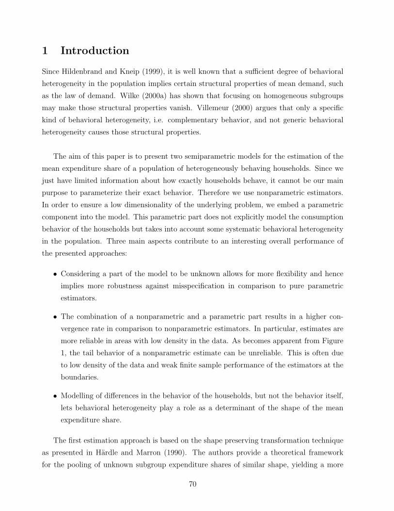
1 Introduction
Since Hildenbrand and Kneip (1999), it is well known that a sufficient degree of behavioral
heterogeneity in the population implies certain structural properties of mean demand, such
as the law of demand. Wilke (2000a) has shown that focusing on homogeneous subgroups
may make those structural properties vanish. Villemeur (2000) argues that only a specific
kind of behavioral heterogeneity, i.e. complementary behavior, and not generic behavioral
heterogeneity causes those structural properties.
The aim of this paper is to present two semiparametric models for the estimation of the
mean expenditure share of a population of heterogeneously behaving households. Since we
just have limited information about how exactly households behave, it cannot be our main
purpose to parameterize their exact behavior. Therefore we use nonparametric estimators.
In order to ensure a low dimensionality of the underlying problem, we embed a parametric
component into the model. This parametric part does not explicitly model the consumption
behavior of the households but takes into account some systematic behavioral heterogeneity
in the population. Three main aspects contribute to an interesting overall performance of
the presented approaches:
• Considering a part of the model to be unknown allows for more flexibility and hence
implies more robustness against misspecification in comparison to pure parametric
estimators.
• The combination of a nonparametric and a parametric part results in a higher con-
vergence rate in comparison to nonparametric estimators. In particular, estimates are
more reliable in areas with low density in the data. As becomes apparent from Figure
1, the tail behavior of a nonparametric estimate can be unreliable. This is often due
to low density of the data and weak finite sample performance of the estimators at the
boundaries.
• Modelling of differences in the behavior of the households, but not the behavior itself,
lets behavioral heterogeneity play a role as a determinant of the shape of the mean
expenditure share.
The first estimation approach is based on the shape preserving transformation technique
as presented in Hardle and Marron (1990). The authors provide a theoretical framework
for the pooling of unknown subgroup expenditure shares of similar shape, yielding a more
70
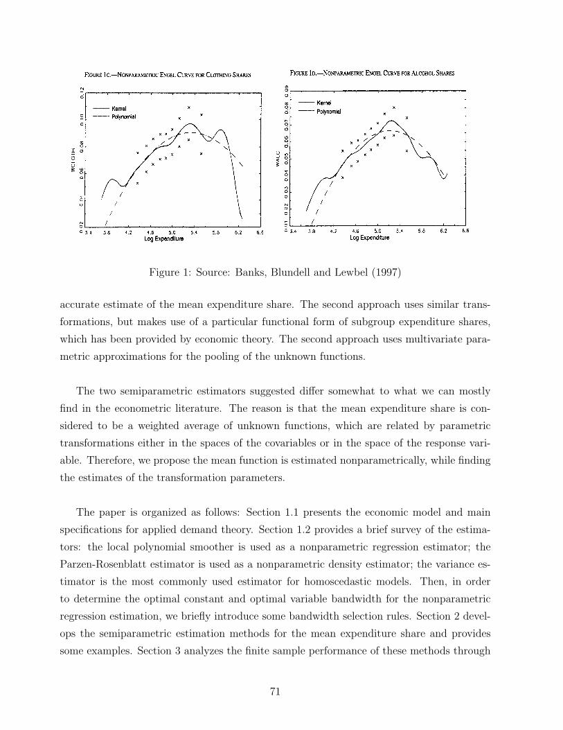
Figure 1: Source: Banks, Blundell and Lewbel (1997)
accurate estimate of the mean expenditure share. The second approach uses similar trans-
formations, but makes use of a particular functional form of subgroup expenditure shares,
which has been provided by economic theory. The second approach uses multivariate para-
metric approximations for the pooling of the unknown functions.
The two semiparametric estimators suggested differ somewhat to what we can mostly
find in the econometric literature. The reason is that the mean expenditure share is con-
sidered to be a weighted average of unknown functions, which are related by parametric
transformations either in the spaces of the covariables or in the space of the response vari-
able. Therefore, we propose the mean function is estimated nonparametrically, while finding
the estimates of the transformation parameters.
The paper is organized as follows: Section 1.1 presents the economic model and main
specifications for applied demand theory. Section 1.2 provides a brief survey of the estima-
tors: the local polynomial smoother is used as a nonparametric regression estimator; the
Parzen-Rosenblatt estimator is used as a nonparametric density estimator; the variance es-
timator is the most commonly used estimator for homoscedastic models. Then, in order
to determine the optimal constant and optimal variable bandwidth for the nonparametric
regression estimation, we briefly introduce some bandwidth selection rules. Section 2 devel-
ops the semiparametric estimation methods for the mean expenditure share and provides
some examples. Section 3 analyzes the finite sample performance of these methods through
71
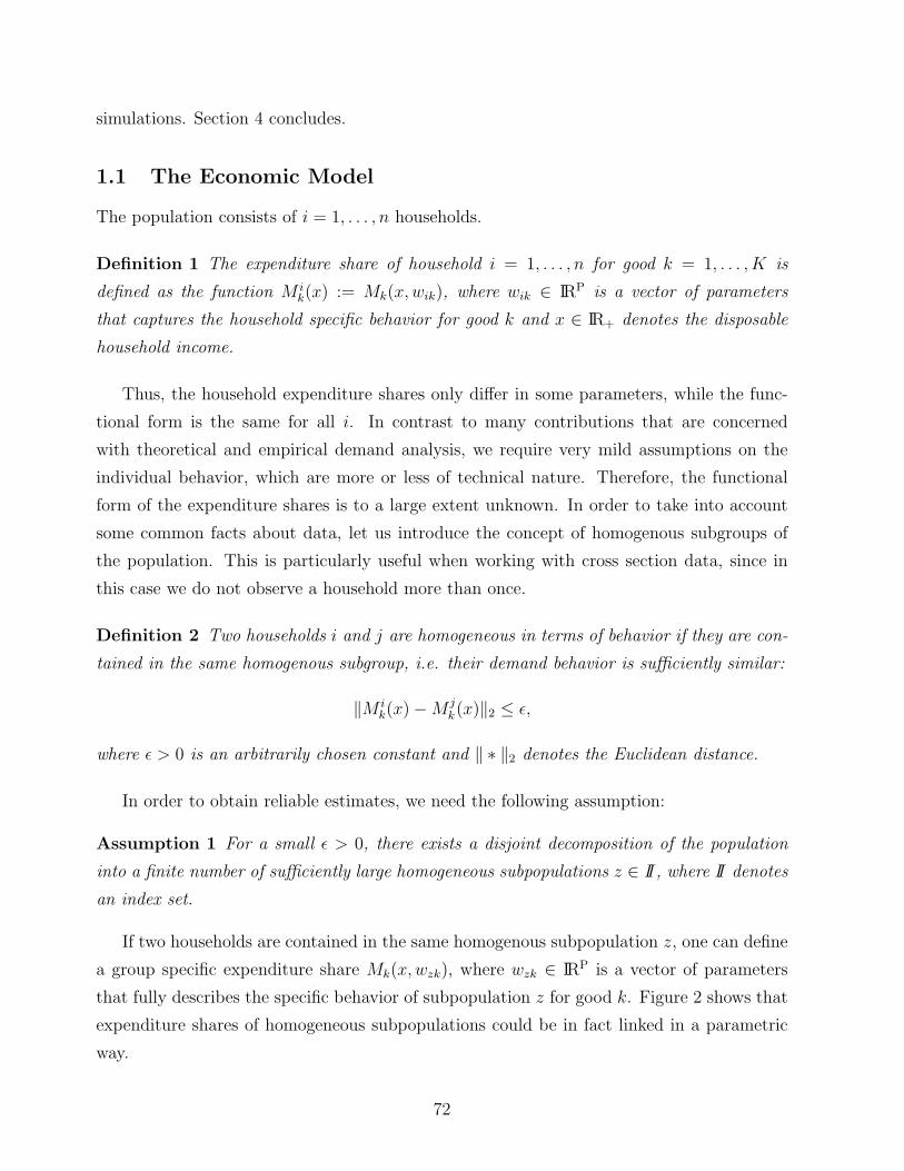
simulations. Section 4 concludes.
1.1 The Economic Model
The population consists of i = 1, . . . , n households.
Definition 1 The expenditure share of household i = 1, . . . , n for good k = 1, . . . , K is
defined as the function M ik(x) := Mk(x,wik), where wik ∈ IRP is a vector of parameters
that captures the household specific behavior for good k and x ∈ IR+ denotes the disposable
household income.
Thus, the household expenditure shares only differ in some parameters, while the func-
tional form is the same for all i. In contrast to many contributions that are concerned
with theoretical and empirical demand analysis, we require very mild assumptions on the
individual behavior, which are more or less of technical nature. Therefore, the functional
form of the expenditure shares is to a large extent unknown. In order to take into account
some common facts about data, let us introduce the concept of homogenous subgroups of
the population. This is particularly useful when working with cross section data, since in
this case we do not observe a household more than once.
Definition 2 Two households i and j are homogeneous in terms of behavior if they are con-
tained in the same homogenous subgroup, i.e. their demand behavior is sufficiently similar:
‖M ik(x)−M j
k(x)‖2 ≤ ε,
where ε > 0 is an arbitrarily chosen constant and ‖ ∗ ‖2 denotes the Euclidean distance.
In order to obtain reliable estimates, we need the following assumption:
Assumption 1 For a small ε > 0, there exists a disjoint decomposition of the population
into a finite number of sufficiently large homogeneous subpopulations z ∈ II, where II denotes
an index set.
If two households are contained in the same homogenous subpopulation z, one can define
a group specific expenditure share Mk(x,wzk), where wzk ∈ IRP is a vector of parameters
that fully describes the specific behavior of subpopulation z for good k. Figure 2 shows that
expenditure shares of homogeneous subpopulations could be in fact linked in a parametric
way.
72
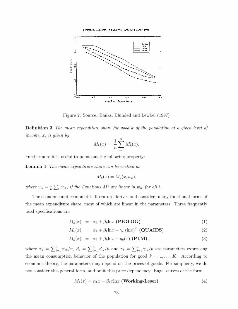
Figure 2: Source: Banks, Blundell and Lewbel (1997)
Definition 3 The mean expenditure share for good k of the population at a given level of
income, x, is given by
Mk(x) :=1
n
n∑i=1
M ik(x).
Furthermore it is useful to point out the following property:
Lemma 1 The mean expenditure share can be written as
Mk(x) = Mk(x, wk),
where wk = 1n
∑i wik, if the Functions M i are linear in wik for all i.
The economic and econometric literature derives and considers many functional forms of
the mean expenditure share, most of which are linear in the parameters. Three frequently
used specifications are
Mk(x) = αk + βklnx (PIGLOG) (1)
Mk(x) = αk + βklnx + γk (lnx)2 (QUAIDS) (2)
Mk(x) = αk + βklnx + gk(x) (PLM), (3)
where αk =∑n
i=1 αik/n, βk =∑n
i=1 βik/n and γk =∑n
i=1 γik/n are parameters expressing
the mean consumption behavior of the population for good k = 1, . . . , K. According to
economic theory, the parameters may depend on the prices of goods. For simplicity, we do
not consider this general form, and omit this price dependency. Engel curves of the form
Mk(x) = αkx + βkxlnx (Working-Leser) (4)
73

have been introduced by Working (1963) and Leser (1943). For some goods, Working and
Leser’s specification is well supported by empirical analysis, as is the PIGLOG specifica-
tion. However, expenditure shares are not generally log-linear. This is in accordance with
Gorman’s (1981) theoretical findings, which showed that utility based exactly aggregable
demand systems have a maximum rank equal to three, where the maximum rank of a de-
mand system is defined as the maximum rank of the (K × P ) matrix of the demand system
coefficients. Here, P denotes the number of parameters in a demand system, i.e. P = 2 in
(4) and (1), and P = 3 in (2). Banks et al. (1997) deal with rank three demand systems.
They show that the Quadratic Almost Ideal Demand System (QUAIDS) is the only rank
three demand system that is consistent with utility maximization and has expenditure shares
which are linear in a constant, in log income and in some other differentiable function of
income. Note that in (1), (2) and (4) Mk is linear in wik.
Since the purpose of this paper is to suggest two new semiparametric methods, we do not
consider mean expenditure shares of the common semiparametric specification (3). These
models are known as partially linear models (PLM) and represent a common extension of the
PIGLOG specification. The function gk(x) is an unknown smooth function that captures
all nonlinearities in x. It is estimated with a nonparametric estimator. Robinson (1988)
has shown√
n-consistency of the parameter estimates, while using the Nadaraya-Watson
estimator as the estimator for gk. Wilke (2000b) compares the Nadaraya-Watson estimator
to the local linear smoother and derives differences in asymptotic properties for both cases.
His simulations indicate that the local linear smoother possesses a superior finite sample
performance in this class of models. For further analysis let us omit the index k, i.e. focus
on one good.
1.2 The Estimators
Local Polynomial Regression Let (X, Y ) be observable random variables with (Xi, Yi)i=1,...,n
independent realizations. Suppose that
E(Y |X) = M(X)
holds, where
Y |X ∼ N(E(Y |X), σ2
)
74

and M is an unknown smooth function of Cν , the space of ν times differentiable functions,
for which the following series around x0 exists
M(X) = M(x0) + M ′(x0)(X − x0) +M ′′(x0)
2!(X − x0)
2 + . . . +M (ν)(x0)
ν!(X − x0)
ν .
Let K : IR 7→ IR be the Kernel function which satisfies:
• ∫K(u)du = 1
• K has compact support and is bounded
• All odd order moments of K vanish, i.e.∫
ulK(u)du = 0
for all odd integers l > 0. This is for example satisfied for symmetric functions.
Under the foregoing regularity conditions on the model and the Kernel function, the local
polynomial regression estimator at the evaluation point x is the solution to
min∑
i
(Yj −
ν∑j=0
aj(Xi − x)j
)2
Kh(Xi − x)
with respect to aj where Kh(Xi − x) = K ((Xi − x)/h(x)) /h(x) and h(x) denotes either a
variable bandwidth or a constant bandwidth h. The natural estimator for M(x0) is a0. In
fact, it is the solution to the following weighted least squares problem:
a = (X′WX)−1X′WY, (5)
where
X =
1 (X1 − x0) . . . (X1 − x0)ν
......
...
1 (Xn − x0) . . . (Xn − x0)ν
, Y =
Y1
...
Yn
, a =
a0
...
aν
and W = diag{Kh(Xi−x0)}. The performance of a0 is better when choosing ν odd. Fan and
Gijbels (1996) give a detailed description of local polynomial modelling and derive adequate
rules in order to choose ν.
Density estimation Under the usual conditions on the marginal density f(X), it is esti-
mated by
f(x) =1
n
∑i
Kh(Xi − x),
which is the so called Parzen-Rosenblatt estimator.
75

Variance estimation The unknown variance σ2 is estimated by
σ2 =∑
i
(Yi − M(Xi)
)2
f(Xi). (6)
Our model can be extended to a heteroscedastic one with an unknown variance function.
In this case the local polynomial variance function estimator of Ruppert, Wand, Holst and
Hossjer (1997) can be used.
Optimal Choice of the Bandwidth The choice of the bandwidth is crucial in nonpara-
metric regression and density estimation. The correct choice of bandwidth is necessary for
obtaining pointwise or uniform consistency of the nonparametric estimators.
Optimality of a bandwidth requires that it minimizes the asymptotic mean integrated
squared error (AMISE) of the estimator. The asymptotically optimal constant bandwidth
for regression function estimation when choosing ν = 1 and using the Epanechnikov-Kernel
is given by
hopt = 1.719
[∫σ2w(x)/f(x)dx∫M ′′(x)2w(x)dx
]1/5
n−1/5, (7)
where w : IR 7→ IR is an arbitrary weight function with∫
IRw(x)dx = 1. The function f
denotes the marginal density of X, whilst x are the design points. To obtain the value of
the constant, refer to Fan and Gijbels (1996). Note that 2a2 may serve as an estimate of
M ′′ and σ2 is an estimate of σ2 as defined in the foregoing paragraph. The optimal variable
bandwidth is proportional to
hopt(x) ∝[
σ2
M ′′(x)2f(x)
]1/5
n−1/5, (8)
where the denominator has to be bounded away from 0 for all x. If the denominator tends
to 0, the optimal constant bandwidth can be chosen. One can show (see Fan and Gijbels
(1992)) that the AMISE when using a constant bandwidth selection is at least the AMISE
when using a variable bandwidth selection. Figure 3c shows the resulting h and h(x), based
on the shape of f(X) (Figure 3a) and M ′′(X) (Figure 3b).
Plug-In Method As a matter of fact, the nonparametric estimators depend on the band-
width, and the optimal bandwidth depends on unknown quantities that have to be estimated.
In turn, these estimates depend upon the initial selection of the bandwidth. Therefore, it is
straightforward to estimate the unknown quantities M , M ′′, h and σ2 in an iterative way:
76
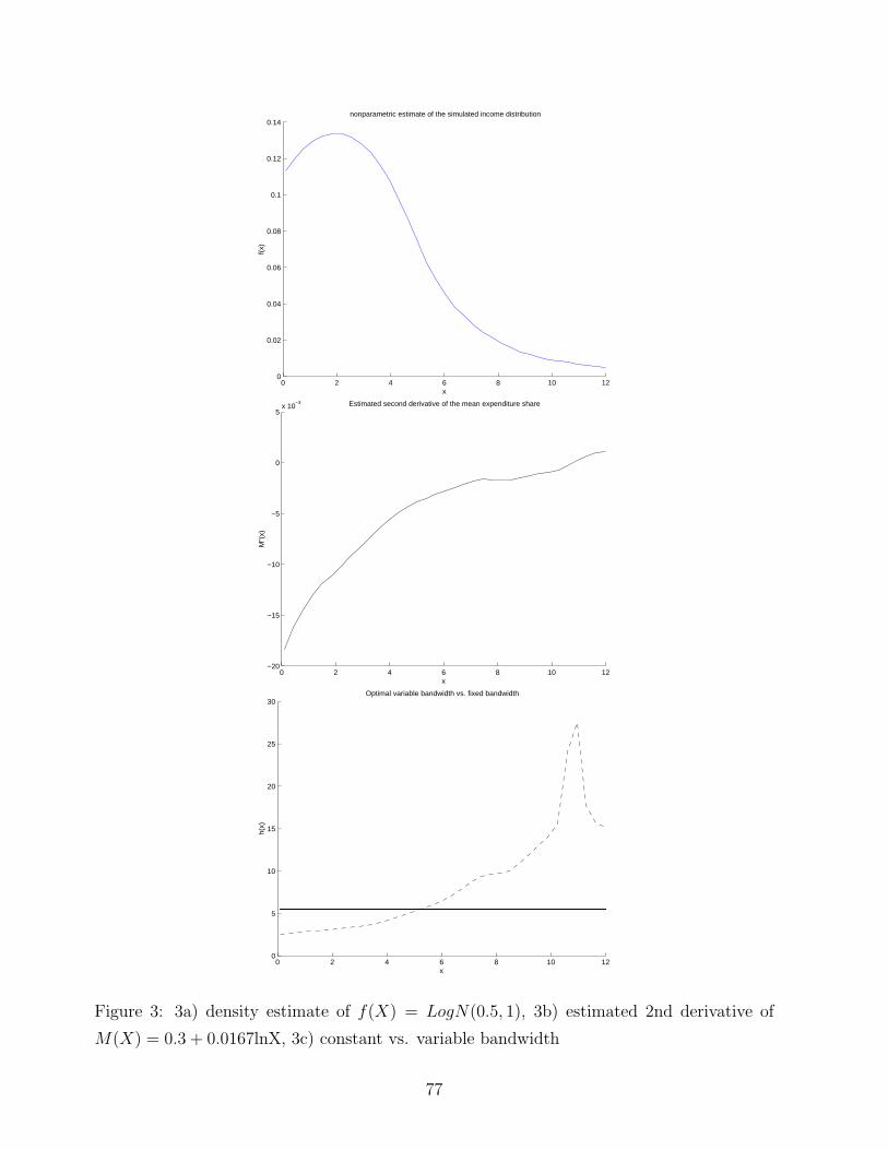
0 2 4 6 8 10 120
0.02
0.04
0.06
0.08
0.1
0.12
0.14nonparametric estimate of the simulated income distribution
f(x)
x
0 2 4 6 8 10 12−20
−15
−10
−5
0
5x 10
−3 Estimated second derivative of the mean expenditure share
M"(
x)
x
0 2 4 6 8 10 120
5
10
15
20
25
30Optimal variable bandwidth vs. fixed bandwidth
h(x)
x
Figure 3: 3a) density estimate of f(X) = LogN(0.5, 1), 3b) estimated 2nd derivative of
M(X) = 0.3 + 0.0167lnX, 3c) constant vs. variable bandwidth
77

1. Crude determination of a bandwidth (h0) by using a rule of thumb.
2. Use this bandwidth in order to estimate the unknown quantities.
3. Compute new bandwidths while using M , M ′′, σ2 and f .
4. Repeat steps 2 and 3 until convergence.
This method has been suggested by for example Fan and Gijbels (1996).
2 Semiparametric Estimation
2.1 Transformation of Covariables
This section presents an estimation procedure for the estimation of a unknown mean regres-
sion function. It captures an idea of Hardle and Marron (1990), who consider similar shaped
regression functions which are related in a parametric way. Shape preserving transformations
of these curves are used to obtain a more accurate final estimate of the regression function,
that makes use of all available data. Accordingly, we describe a method that allows for
pooling subsamples in order to obtain a more precise nonparametric estimate of the mean
regression function.
Suppose (X,Y, Z) are observable random variables with (Xi, Yi, Zi)i=1,...,n ∈ IR × IR×II
independent realizations. There are two independent covariates: let X denote the household
income and Z denote an index devoted to a homogeneous subgroup z of the households
i. Hence card{II} is the number of homogeneous subgroups. Furthermore let the following
equation hold:
E(Y |X, Z) = AZ (m(TZ(X))) , (9)
where AZ : IR 7→ IR and TZ : IR 7→ IR are known bijective transformation functions
with unknown parameter vectors αz and βz respectively. Note that the unknown func-
tion m ∈ Cν : IR 7→ IR does not depend on Z, where ν denotes a positive integer.
In general, the underlying model (9) can be used to combine univariate data sets that
are linked via shape invariant or by shape preserving transformations. The subsamples may
represent either the results of experiments or disaggregated subsamples of a larger data set,
i.e. homogeneous subgroups of households (Figure 2).
78

Before going into the details of the estimation, it is necessary to shed some light on the
transformation functions and on the discrete covariable Z. The parameter of the transforma-
tion functions differs in z. Therefore one has card{II} vectors of unknown parameters. For
reasons of identification it is indispensable either to have prior information on the parameter
values for one z ∈ II or to assume ‖α‖ = ‖β‖ = 1. Let us consider the first case and denote
z0 as the corresponding z. It will serve as a basis for the transformations. It is reasonable, if
possible, to take the basis such that the transformation functions AZ and TZ are the identity
functions. Then, the relationship (9) simplifies to
E(Y |X, Z = z0) = m(X).
We require one additional assumption on the structure of the model:
Assumption 2 A−1Z (Y |X, Z) ∼ N
(E(A−1
Z (Y |X,Z)), σ2Z
)
This assumption ensures the applicability of usual (weighted) least squares estimation.
Remark 1 The conditional density functions of X|Z are independent of Z, i.e. f(X|Z) =
f(X), ∀Z. This is due to the independency of X and Z.
Assumption 3 If Tz(x) is not the identity function for all z ∈ II, the function m has to be
nonlinear and noncycling on its observed support. Moreover the parameter space of β has to
be restricted to some extent in order to ensure that the nonparametric estimates are indeed
comparable on the same support.
A discussion of Assumption 3 can be found in Wilke (2001) for a similar class of models.
Suppose that Assumptions 1, 2, 3, the regularity conditions on the model and on the Kernel
function hold. A five step estimation procedure in order to estimate the mean regression
function M(X) is presented in what follows:
1. For all z ∈ II and all admissible αz and βz, determine Tz(X) and A−1z (Y ).
2. Estimate m(Tz(X)) by minimizing
∑
i|Zi=z
(A−1
z (Yi)−ν∑
j=0
aj (Tz(Xi)− s)j
)2
Kh (s− Tz(Xi))
with respect to aj for all z, αz and βz, where s are the design points. Consequently,
a0 = mαz ,βz .
79
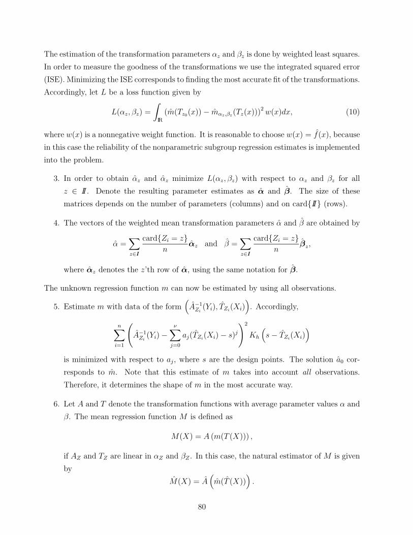
The estimation of the transformation parameters αz and βz is done by weighted least squares.
In order to measure the goodness of the transformations we use the integrated squared error
(ISE). Minimizing the ISE corresponds to finding the most accurate fit of the transformations.
Accordingly, let L be a loss function given by
L(αz, βz) =
∫
IR
(m(Tz0(x))− mαz ,βz(Tz(x)))2 w(x)dx, (10)
where w(x) is a nonnegative weight function. It is reasonable to choose w(x) = f(x), because
in this case the reliability of the nonparametric subgroup regression estimates is implemented
into the problem.
3. In order to obtain αz and αz minimize L(αz, βz) with respect to αz and βz for all
z ∈ II. Denote the resulting parameter estimates as α and β. The size of these
matrices depends on the number of parameters (columns) and on card{II} (rows).
4. The vectors of the weighted mean transformation parameters α and β are obtained by
α =∑z∈II
card{Zi = z}n
αz and β =∑z∈II
card{Zi = z}n
βz,
where αz denotes the z’th row of α, using the same notation for β.
The unknown regression function m can now be estimated by using all observations.
5. Estimate m with data of the form(A−1
Zi(Yi), TZi
(Xi)). Accordingly,
n∑i=1
(A−1
Zi(Yi)−
ν∑j=0
aj(TZi(Xi)− s)j
)2
Kh
(s− TZi
(Xi))
is minimized with respect to aj, where s are the design points. The solution a0 cor-
responds to m. Note that this estimate of m takes into account all observations.
Therefore, it determines the shape of m in the most accurate way.
6. Let A and T denote the transformation functions with average parameter values α and
β. The mean regression function M is defined as
M(X) = A (m(T (X))) ,
if AZ and TZ are linear in αZ and βZ . In this case, the natural estimator of M is given
by
M(X) = A(m(T (X))
).
80
Using the full sample size for the final nonparametric estimate is the main advantage of this
approach. Asymptotic properties are not treated in detail here but consistency can be shown
using the same framework as in Wilke (2001): under appropriate regularity conditions on
the model and the bandwidth selection rule, the nonparametric estimators are uniformly
consistent. The consistency of the parametric estimator can then be shown by using the
nonlinear least squares estimation framework.
The above defined estimation procedure can also perform well in the case of similarly
shaped regression functions mz, i.e. limited dependency on z:
‖mz0(x)−mz(x)‖2 ≤ ε
for all z ∈ II, where ε ≥ 0 is an arbitrarily chosen constant. The trade-off is as follows: Using
all data improves the identification of m, but combining different functions may result in a
biased estimate of the parameters. For further details see for example Pinkse and Robinson
(1995).
2.2 Examples
Hardle and Marron (1990) and Pinkse and Robinson (1995) Hardle and Marron
(1990) consider the following example. It treats transformations of the vertical axis and the
horizontal axis. In particular, they consider
TZ(X) = X + βZ and AZ (m(TZ(X))) = m(TZ(X)) + αZ .
Consequently, the matrices of unknown parameters reduce to vectors and therefore α and β,
the vectors of average transformation parameters, consist of only one element.
Hardle and Marron have shown consistency and asymptotic normality of the resulting
parameter estimates when using the Nadaraya-Watson Kernel estimator with nonstochastic
regressors. Moreover, they derived asymptotic results for a wider class of transformation
functions that are also treated in the next example.
Pinkse and Robinson consider shape preserving transformation functions in a stochastic
regressors framework. Let A be an affine transformation function that is taken to be
AZ(m) = α1,Z + α2,Zm(TZ(x))
81

and let TZ(X) be an invertible transformation function with unknown parameters β. The
loss function for Z = z is therefore given by
L(α1,z, α2,z, βz) =
∫
IR
(m(Tz0(x))− α1,z − α2,z(mαz ,βz(Tz(x))))2 w(x)dx
and the final estimate of m is obtained by minimizing
n∑i=1
(Yi − α1,Zi
α2,Zi
−ν∑
j=0
aj(TZi(Xi)− s)j
)2
Kh
(s− TZi
(Xi))
with respect to aj.
Pinkse and Robinson have shown√
n-consistency and asymptotic normality of the pa-
rameter estimates α1, α2 and β. However, in their paper they have chosen a specification
of the loss function that is based on the definition of the Nadaraya-Watson estimator and
different to what we have presented here. As shown in Wilke (2001) by simulations, the fi-
nite sample performance of an estimator using their particular specification is worse in many
applications, because it can involve larger expected bias of the nonparametric estimators.
PIGLOG expenditure shares Suppose that although economic theory proposes that
Engel curves are of the PIGLOG form as given in (1), there is little faith in this specification.
In particular, the specification m(x) =lnx seems too specific. Therefore, we intend to identify
the shape of m(x) with the help of a nonparametric estimator. Accordingly, we assume
M(X, Z) = AZ (m(X)) = α1,Z + α2,Zm(X),
where the function T is now the identity function and A is an affine transformation function.
Therefore we have a special case of the Pinkse and Robinson model and equivalent asymptotic
properties of the parameter estimates can be inferred immediately. In order to estimate m,
we have to minimize
n∑i=1
(Yi − α1,Zi
α2,Zi
−ν∑
j=0
aj(Xi − x)j
)2
Kh (x−Xi)
with respect to aj. Note that for this and the following example we require Assumption 3.
PIGLOG expenditure shares with price dependency Suppose that the population
is homogenous, i.e. there is only one subgroup, and we observe this group at various dates.
By definition, panel data fulfills this condition, but cross section may satisfy it, too. Assume
82

that the expenditure share of this group depends on time due to price variation, for example.
The model can then be written as
M(X, Z) = AZ (m(X)) = α1,Z + α2,Zm(X),
where Z = Zi now represents an observation date Zi ∈ II. One may also combine this spec-
ification with the modelling of heterogeneity. Then, we have expenditure shares depending
on time and subgroup specific behavior.
2.3 Semiparametric fitting of basis functions
In this section, the regression function is assumed to satisfy
E(Y |X,Z) = m (X, Z) , (11)
where X ∈ IR and Z ∈ II, the covariables, are again independent observable random variables
with i = 1, . . . , n independent realizations. The function m ∈ Cν : IR× II 7→ IR is an unknown
function which does not necessarily have the bijective property. Let Xi denote the income
of a household and let Zi denote the index devoted to its homogeneous subgroup. In order
to keep things simple, let us again assume
Y |X, Z ∼ N(E(Y |X,Z), σ2
z
)
and remark that f(X|Z) = f(X) as in the previous approach.
The idea of this section is to approximate the function m by a linear combination of
a known basis function T : IR 7→ IRP, which has an image of full rank, and unknown
transformation parameters tz ∈ IRP:
m(X|Z) ≈ t′ZT (X)
where P , the dimension of the approximation, determines the degree of smoothing and should
in fact be the rank of the underlying demand system. In many cases the basis functions can
be chosen by reference to a guess that has been provided by theoretical analysis. Ramsay
and Silverman (1997) call this approach “fitting of basis functions”. Like in Section (2.1),
the first aim is to estimate the values of the transformation parameters tz. Using matrix
notation, the least squares estimator for tz is given by
tz = (T′zTz)
−1T′zYz (12)
83
where Tz is the card{II} × P matrix of basis function values with T (Xi)′ as the i’th row
such that Zi = z. Yz denotes the card{Zi = z}×1 vector of Yi|Zi = z. Note that Tz has full
rank. There is obviously some relationship to the loss function criterion from the previous
section, since we are minimizing the norm ‖Yz −Tztz‖2. Moreover, this estimator can easily
be adjusted by a weighting scheme. The corresponding loss function is then given by
L(tz) =
∫
IR
(mz(x)− t′zT (x))2w(x)dx,
where mz(x) is a nonparametric estimate of m(x, z). As already mentioned in the previous
section, we propose a nonparametric estimate of the marginal density of x as a weight
function. Minimizing the loss function is equivalent to minimizing the weighted norm. The
weighted least squares estimator for tz can therefore be written as
tz = (T′zWTz)
−1T′zWmz
where Tz is the same as in (12) and W denotes the matrix of weights. Note that W does
not depend on z. Solving the equation for all z ∈ II yields t, the card{II} × P matrix of
parameter estimates.
In order to estimate the mean regression function, we have to compute the averaged
estimated transformation parameters t as in the foregoing section. Then, we are able to
transform the data to the mean level before estimating the mean regression function, M(X),
with the local polynomial smoother by using all observations.
Example: QUAIDS Suppose we have a model of the form
E(Y |X, Z) := t1Z + t2Z lnX + t3Z(lnX)2
where Y ∼ N(E(Y |X,Z), σ2Z). Accordingly, T (X)′ = (1 lnX (lnX)2), t′z = (t1z t2z t3z) and
P = 3. The mean regression function is given by
M(X) = t1 + t2lnX + t3(lnX)2
where
tp =∑z∈II
card{Z = z}n
tzp for p = 1, 2, 3.
The loss function now becomes
L(tz) =
∫
IR
(mz(x)− t1z − t2zlnx− t3z(lnx)2
)2w(x)dx.
84
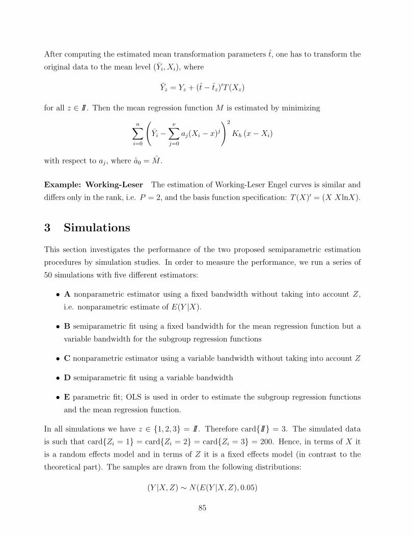
After computing the estimated mean transformation parameters t, one has to transform the
original data to the mean level (Yi, Xi), where
Yz = Yz + (t− tz)′T (Xz)
for all z ∈ II. Then the mean regression function M is estimated by minimizing
n∑i=0
(Yi −
ν∑j=0
aj(Xi − x)j
)2
Kh (x−Xi)
with respect to aj, where a0 = M .
Example: Working-Leser The estimation of Working-Leser Engel curves is similar and
differs only in the rank, i.e. P = 2, and the basis function specification: T (X)′ = (X XlnX).
3 Simulations
This section investigates the performance of the two proposed semiparametric estimation
procedures by simulation studies. In order to measure the performance, we run a series of
50 simulations with five different estimators:
• A nonparametric estimator using a fixed bandwidth without taking into account Z,
i.e. nonparametric estimate of E(Y |X).
• B semiparametric fit using a fixed bandwidth for the mean regression function but a
variable bandwidth for the subgroup regression functions
• C nonparametric estimator using a variable bandwidth without taking into account Z
• D semiparametric fit using a variable bandwidth
• E parametric fit; OLS is used in order to estimate the subgroup regression functions
and the mean regression function.
In all simulations we have z ∈ {1, 2, 3} = II. Therefore card{II} = 3. The simulated data
is such that card{Zi = 1} = card{Zi = 2} = card{Zi = 3} = 200. Hence, in terms of X it
is a random effects model and in terms of Z it is a fixed effects model (in contrast to the
theoretical part). The samples are drawn from the following distributions:
(Y |X, Z) ∼ N(E(Y |X,Z), 0.05)
85
and
f(X) = LogN(0.5, 1).
Matlab 5.3 serves as the software environment. We use the random number generators of
the toolbox ‘Statistics’. All non- and semiparametric estimators are self- programmed.
In order to investigate the performance of the Methods A-E, we apply them in six different
models:
True Model Specification
1. PIGLOG (Example of Section 2.2) ⇒ Table 1, Figure 4
2. QUAIDS, (Example of Section 2.3) ⇒ Table 2, Figure 5
Misspecification
3. Specification: QUAIDS
True Model: PIGLOG ⇒ Table 3, Figure 6
4. Specification: PIGLOG
True Model: QUAIDS ⇒ Table 4, Figure 7
5. Specification: QUAIDS
True Model: PIGLOG with an additional sine-function ⇒ Table 5, Figure 8
6. Specification: PIGLOG
True Model: PIGLOG with an additional sine-function ⇒ Table 6, Figure 9
The true values of the transformation parameters differ across the six models as is apparent
from the tables.
Resulting Performance In order to measure the performance of the estimators A-E, the
mean averaged squared error (MASE) is used:
MASE =1
S
S∑s=1
MSE(s) =1
S
S∑s=1
[(EM(s)−M(s)
)2
+ var(M(s))
],
where s ∈ (0, 12] denote the evaluation points. The nonparametric regression function esti-
mates are obtained with the local polynomial smoother, where ν is always chosen to be one
86

(local linear smoother), except for the estimation of the second derivative of the regression
function, which is done with ν = 3.
Tables 1-6 and Figures 4-9 present the results of the finite sample performance of the
methods. The following list summarizes the main findings:
• The nonparametric estimators A and C have serious problems in areas with low density
in the data, e.g. relatively rich people. This is in accordance with the empirical findings
of Banks et al. (1997) (see Figure 1). In addition, estimator A in Case 4 indicates a
linear underlying model structure, but in fact the true model is far linear. However,
estimators A and C would become more precise by increasing the sample size.
• The parametric estimator E is biased in the case of misspecification. In this case, it is
unable to detect the true underlying model structure. Under the true model specifi-
cation it outperforms the other estimators since the rate of convergence of parametric
estimators is higher.
• The choice of a variable bandwidth in five cases results in a lower MASE than choosing
a fixed bandwidth. Therefore estimator D should be preferred over B, and C over A.
This is in accordance with the theoretical findings of Fan and Gijbels (1992).
• Considering all model specifications, estimator D appears to be a good choice for the
estimation of mean expenditure shares.
87
4 Conclusion
Two semiparametric approaches to the estimation of mean expenditure shares have been
presented and have been compared to usual parametric and nonparametric methods. It is
well known that parametric estimators perform best if the underlying model specification
is correct, otherwise they are not consistent. Nonparametric estimators are consistent for
a broader class of models but require more observation in order to obtain precise results.
They have a poor performance in areas with low density in the data. The simulation study
shows that the two suggested semiparametric estimators reduce these main disadvantages.
They are more flexible than parametric estimators and have a higher convergence rate than
nonparametric estimators. The latter is of particular importance when working with small
samples. The simulations attest this aspect of finite sample performance of the estimators.
In addition, the simulations indicate that choosing a variable bandwidth is superior to choos-
ing a fixed bandwidth.
It remains to conclude that the proposed methods for the modelling of behavioral hetero-
geneity perform well in finite samples. Hence, the econometrician is not obliged to suppose
household behavior as a result of utility maximization. Behavioral heterogeneity need no
longer be considered a burden, but rather an important determinant of the mean expenditure
share.
88
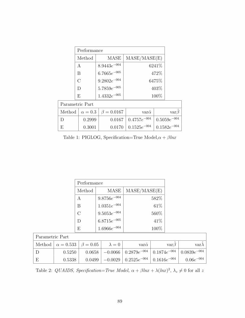
Performance
Method MASE MASE/MASE(E)
A 8.9443e−004 6241%
B 6.7665e−005 472%
C 9.2802e−004 6475%
D 5.7859e−005 403%
E 1.4332e−005 100%
Parametric Part
Method α = 0.3 β = 0.0167 varα varβ
D 0.2999 0.0167 0.4757e−004 0.5059e−004
E 0.3001 0.0170 0.1525e−004 0.1582e−004
Table 1: PIGLOG, Specification=True Model,α + βlnx
Performance
Method MASE MASE/MASE(E)
A 9.8756e−004 582%
B 1.0351e−004 61%
C 9.5053e−004 560%
D 6.8715e−005 41%
E 1.6966e−004 100%
Parametric Part
Method α = 0.533 β = 0.05 λ = 0 varα varβ varλ
D 0.5250 0.0658 −0.0066 0.2879e−004 0.1874e−004 0.0839e−004
E 0.5338 0.0499 −0.0029 0.2525e−004 0.1616e−004 0.06e−004
Table 2: QUAIDS, Specification=True Model, α + βlnx + λ(lnx)2, λz 6= 0 for all z
89
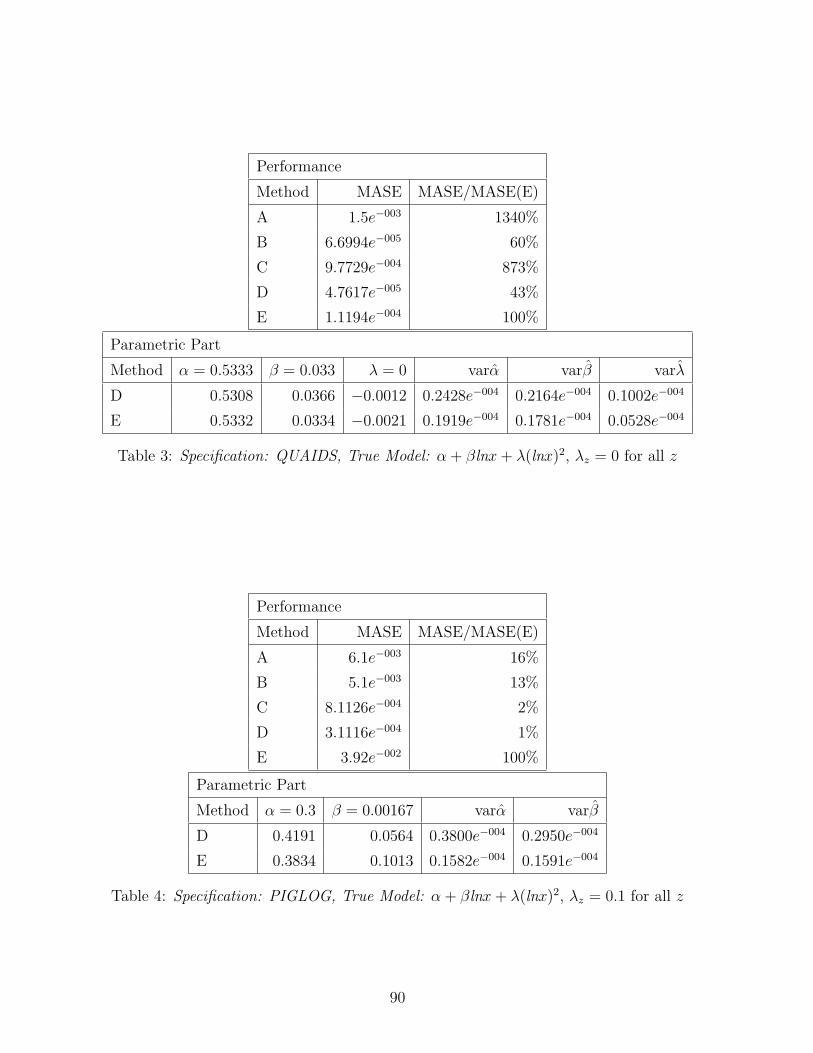
Performance
Method MASE MASE/MASE(E)
A 1.5e−003 1340%
B 6.6994e−005 60%
C 9.7729e−004 873%
D 4.7617e−005 43%
E 1.1194e−004 100%
Parametric Part
Method α = 0.5333 β = 0.033 λ = 0 varα varβ varλ
D 0.5308 0.0366 −0.0012 0.2428e−004 0.2164e−004 0.1002e−004
E 0.5332 0.0334 −0.0021 0.1919e−004 0.1781e−004 0.0528e−004
Table 3: Specification: QUAIDS, True Model: α + βlnx + λ(lnx)2, λz = 0 for all z
Performance
Method MASE MASE/MASE(E)
A 6.1e−003 16%
B 5.1e−003 13%
C 8.1126e−004 2%
D 3.1116e−004 1%
E 3.92e−002 100%
Parametric Part
Method α = 0.3 β = 0.00167 varα varβ
D 0.4191 0.0564 0.3800e−004 0.2950e−004
E 0.3834 0.1013 0.1582e−004 0.1591e−004
Table 4: Specification: PIGLOG, True Model: α + βlnx + λ(lnx)2, λz = 0.1 for all z
90

Performance
Method MASE MASE/MASE(E)
A 2.37e−002 527%
B 8.0753e−004 18%
C 2.14e−002 476%
D 3.0088e−004 7%
E 4.5e−003 100%
Parametric Part
Method α = 0.5333 β = 0.0333 λ = 0 varα varβ varλ
D 0.6050 0.0238 −0.0240 0.3447e−004 0.7777e−004 0.2316e−004
E 0.5981 0.0240 −0.0119 0.1677e−004 0.1762e−004 0.0539e−004
Table 5: Specification: QUAIDS, True Model: α + βlnx + λ(lnx)2+0.1sinx, λz = 0 for all z
Performance
Method MASE MASE/MASE(E)
A 47.7e−003 96%
B 1.7e−003 35%
C 4.5e−003 92%
D 9.4963e−004 19%
E 4.9e−003 100%
Parametric Part
Method α = 0.5 β = 0.0167 varα varβ
D 0.5402 0.0018 0.6281e−004 0.6281e−004
E 0.5564 −0.0077 0.1839e−004 0.1434e−004
Table 6: Specification: PIGLOG, True Model: α + βlnx + 0.1sinx
91
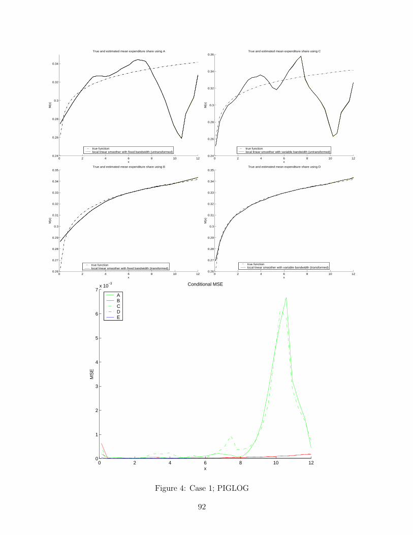
0 2 4 6 8 10 120.24
0.26
0.28
0.3
0.32
0.34
True and estimated mean expenditure share using AM
(x)
x
true function local linear smoother with fixed bandwidth (untransformed)
0 2 4 6 8 10 120.24
0.26
0.28
0.3
0.32
0.34
0.36True and estimated mean expenditure share using C
M(x
)
x
true function local linear smoother with variable bandwidth (untransformed)
0 2 4 6 8 10 120.26
0.27
0.28
0.29
0.3
0.31
0.32
0.33
0.34
0.35True and estimated mean expenditure share using B
M(x
)
x
true function local linear smoother with fixed bandwidth (transformed)
0 2 4 6 8 10 120.26
0.27
0.28
0.29
0.3
0.31
0.32
0.33
0.34
0.35True and estimated mean expenditure share using D
M(x
)
x
true function local linear smoother with variable bandwidth (transformed)
0 2 4 6 8 10 120
1
2
3
4
5
6
7x 10
−3 Conditional MSE
MS
E
x
ABCDE
Figure 4: Case 1; PIGLOG
92
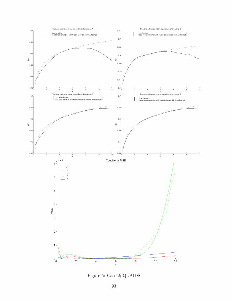
0 2 4 6 8 10 120.45
0.5
0.55
0.6
0.65
0.7True and estimated mean expenditure share using A
M(x
)
x
true function local linear smoother with fixed bandwidth (untransformed)
0 2 4 6 8 10 120.4
0.45
0.5
0.55
0.6
0.65
0.7
0.75True and estimated mean expenditure share using C
M(x
)
x
true function local linear smoother with variable bandwidth (untransformed)
0 2 4 6 8 10 120.45
0.5
0.55
0.6
0.65
0.7True and estimated mean expenditure share using B
M(x
)
x
true function local linear smoother with fixed bandwidth (transformed)
0 2 4 6 8 10 120.45
0.5
0.55
0.6
0.65
0.7True and estimated mean expenditure share using D
M(x
)
x
true function local linear smoother with variable bandwidth (transformed)
0 2 4 6 8 10 120
1
2
3
4
5
6
7x 10
−3 Conditional MSE
MS
E
x
ABCDE
Figure 5: Case 2; QUAIDS
93
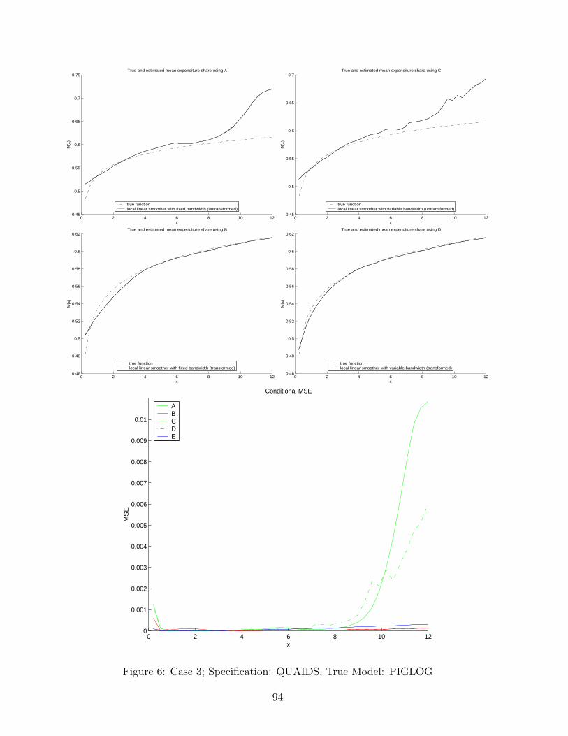
0 2 4 6 8 10 120.45
0.5
0.55
0.6
0.65
0.7
0.75True and estimated mean expenditure share using A
M(x
)
x
true function local linear smoother with fixed bandwidth (untransformed)
0 2 4 6 8 10 120.45
0.5
0.55
0.6
0.65
0.7True and estimated mean expenditure share using C
M(x
)
x
true function local linear smoother with variable bandwidth (untransformed)
0 2 4 6 8 10 120.46
0.48
0.5
0.52
0.54
0.56
0.58
0.6
0.62True and estimated mean expenditure share using B
M(x
)
x
true function local linear smoother with fixed bandwidth (transformed)
0 2 4 6 8 10 120.46
0.48
0.5
0.52
0.54
0.56
0.58
0.6
0.62True and estimated mean expenditure share using D
M(x
)
x
true function local linear smoother with variable bandwidth (transformed)
0 2 4 6 8 10 120
0.001
0.002
0.003
0.004
0.005
0.006
0.007
0.008
0.009
0.01
Conditional MSE
MS
E
x
ABCDE
Figure 6: Case 3; Specification: QUAIDS, True Model: PIGLOG
94

0 2 4 6 8 10 120.3
0.4
0.5
0.6
0.7
0.8
0.9
1
1.1True and estimated mean expenditure share using A
M(x
)
x
true function local linear smoother with fixed bandwidth (untransformed)
0 2 4 6 8 10 120.2
0.3
0.4
0.5
0.6
0.7
0.8
0.9
1
1.1
1.2True and estimated mean expenditure share using C
M(x
)
x
true function local linear smoother with variable bandwidth (untransformed)
0 2 4 6 8 10 120.3
0.4
0.5
0.6
0.7
0.8
0.9
1True and estimated mean expenditure share using B
M(x
)
x
true function local linear smoother with fixed bandwidth (transformed)
0 2 4 6 8 10 120.3
0.4
0.5
0.6
0.7
0.8
0.9
1True and estimated mean expenditure share using D
M(x
)
x
true function local linear smoother with variable bandwidth (transformed)
0 2 4 6 8 10 120
0.05
0.1
0.15
0.2
0.25
0.3
0.35
0.4Conditional MSE
MS
E
x
ABCDE
Figure 7: Case 4; Specification: PIGLOG, True Model: QUAIDS
95
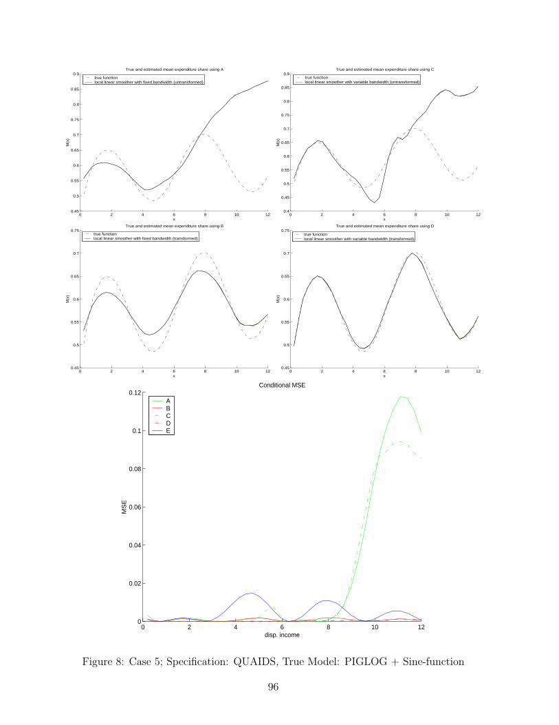
0 2 4 6 8 10 120.45
0.5
0.55
0.6
0.65
0.7
0.75
0.8
0.85
0.9True and estimated mean expenditure share using A
M(x
)
x
true function local linear smoother with fixed bandwidth (untransformed)
0 2 4 6 8 10 120.4
0.45
0.5
0.55
0.6
0.65
0.7
0.75
0.8
0.85
0.9True and estimated mean expenditure share using C
M(x
)
x
true function local linear smoother with variable bandwidth (untransformed)
0 2 4 6 8 10 120.45
0.5
0.55
0.6
0.65
0.7
0.75True and estimated mean expenditure share using B
M(x
)
x
true function local linear smoother with fixed bandwidth (transformed)
0 2 4 6 8 10 120.45
0.5
0.55
0.6
0.65
0.7
0.75True and estimated mean expenditure share using D
M(x
)
x
true function local linear smoother with variable bandwidth (transformed)
0 2 4 6 8 10 120
0.02
0.04
0.06
0.08
0.1
0.12Conditional MSE
MS
E
disp. income
ABCDE
Figure 8: Case 5; Specification: QUAIDS, True Model: PIGLOG + Sine-function
96
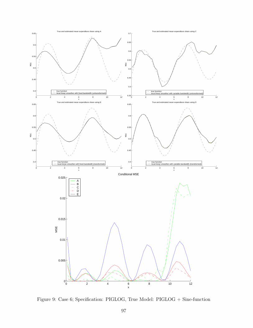
0 2 4 6 8 10 12
0.4
0.45
0.5
0.55
0.6
0.65True and estimated mean expenditure share using A
M(x
)
x
true function local linear smoother with fixed bandwidth (untransformed)
0 2 4 6 8 10 120.35
0.4
0.45
0.5
0.55
0.6
0.65
0.7True and estimated mean expenditure share using C
M(x
)
x
true function local linear smoother with variable bandwidth (untransformed)
0 2 4 6 8 10 12
0.4
0.45
0.5
0.55
0.6
0.65True and estimated mean expenditure share using B
M(x
)
x
true function local linear smoother with fixed bandwidth (transformed)
0 2 4 6 8 10 12
0.4
0.45
0.5
0.55
0.6
0.65True and estimated mean expenditure share using D
M(x
)
x
true function local linear smoother with variable bandwidth (transformed)
0 2 4 6 8 10 120
0.005
0.01
0.015
0.02
0.025Conditional MSE
MS
E
x
ABCDE
Figure 9: Case 6; Specification: PIGLOG, True Model: PIGLOG + Sine-function
97
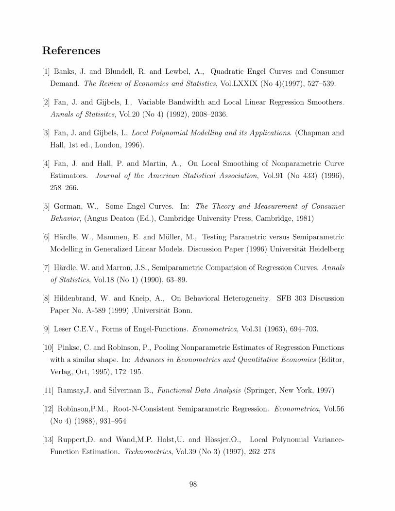
References
[1] Banks, J. and Blundell, R. and Lewbel, A., Quadratic Engel Curves and Consumer
Demand. The Review of Economics and Statistics, Vol.LXXIX (No 4)(1997), 527–539.
[2] Fan, J. and Gijbels, I., Variable Bandwidth and Local Linear Regression Smoothers.
Annals of Statisitcs, Vol.20 (No 4) (1992), 2008–2036.
[3] Fan, J. and Gijbels, I., Local Polynomial Modelling and its Applications. (Chapman and
Hall, 1st ed., London, 1996).
[4] Fan, J. and Hall, P. and Martin, A., On Local Smoothing of Nonparametric Curve
Estimators. Journal of the American Statistical Association, Vol.91 (No 433) (1996),
258–266.
[5] Gorman, W., Some Engel Curves. In: The Theory and Measurement of Consumer
Behavior, (Angus Deaton (Ed.), Cambridge University Press, Cambridge, 1981)
[6] Hardle, W., Mammen, E. and Muller, M., Testing Parametric versus Semiparametric
Modelling in Generalized Linear Models. Discussion Paper (1996) Universitat Heidelberg
[7] Hardle, W. and Marron, J.S., Semiparametric Comparision of Regression Curves. Annals
of Statistics, Vol.18 (No 1) (1990), 63–89.
[8] Hildenbrand, W. and Kneip, A., On Behavioral Heterogeneity. SFB 303 Discussion
Paper No. A-589 (1999) ,Universitat Bonn.
[9] Leser C.E.V., Forms of Engel-Functions. Econometrica, Vol.31 (1963), 694–703.
[10] Pinkse, C. and Robinson, P., Pooling Nonparametric Estimates of Regression Functions
with a similar shape. In: Advances in Econometrics and Quantitative Economics (Editor,
Verlag, Ort, 1995), 172–195.
[11] Ramsay,J. and Silverman B., Functional Data Analysis (Springer, New York, 1997)
[12] Robinson,P.M., Root-N-Consistent Semiparametric Regression. Econometrica, Vol.56
(No 4) (1988), 931–954
[13] Ruppert,D. and Wand,M.P. Holst,U. and Hossjer,O., Local Polynomial Variance-
Function Estimation. Technometrics, Vol.39 (No 3) (1997), 262–273
98
[14] Villemeur, E.B. , Behavioral Complementarity (not heterogeneity) Causes the Law of
Demand.. Manuscript (2000), Universite de Sciences Sociales Toulouse.
[15] Wilke, R. , A Note on Behavioral Heterogeneity and Aggregation. Discussion Paper in
Economics No. 00-05 (2000a), Universitat Dortmund.
[16] Wilke, R., Multivariate Quasi Likelihood Estimation. Discussion Paper in Economics
No. 00-08 (2000b), Universitat Dortmund.
[17] Wilke, R., Semiparametric Estimation of Regression Functions under Shape Invariance
Restrictions. mimeo, University College London.
[18] Working, H., Statistical Laws of Family Expenditure. Journal of the American Statis-
tical Association, Vol.38 (1943), 43–56
99
Essay 5
Semiparametric Estimation of Regression Functions
Under Shape Invariance Restrictions
April 22, 2002
Abstract
This paper considers the shape invariant modelling approach in semiparametric
regression estimation. Nonparametric regression functions of similar shape are linked
by parametric transformations with unknown parameters. A computationally conve-
nient estimation procedure is suggested. Finite sample performance of this estimator
is investigated by simulations. Consistency of the parameter estimates is shown. An
application to consumer data illustrates the importance of this method for applied
statistics. Estimation results indicate that the imposed shape invariance restrictions
have empirical evidence in the semiparametric modelling of consumer demand.
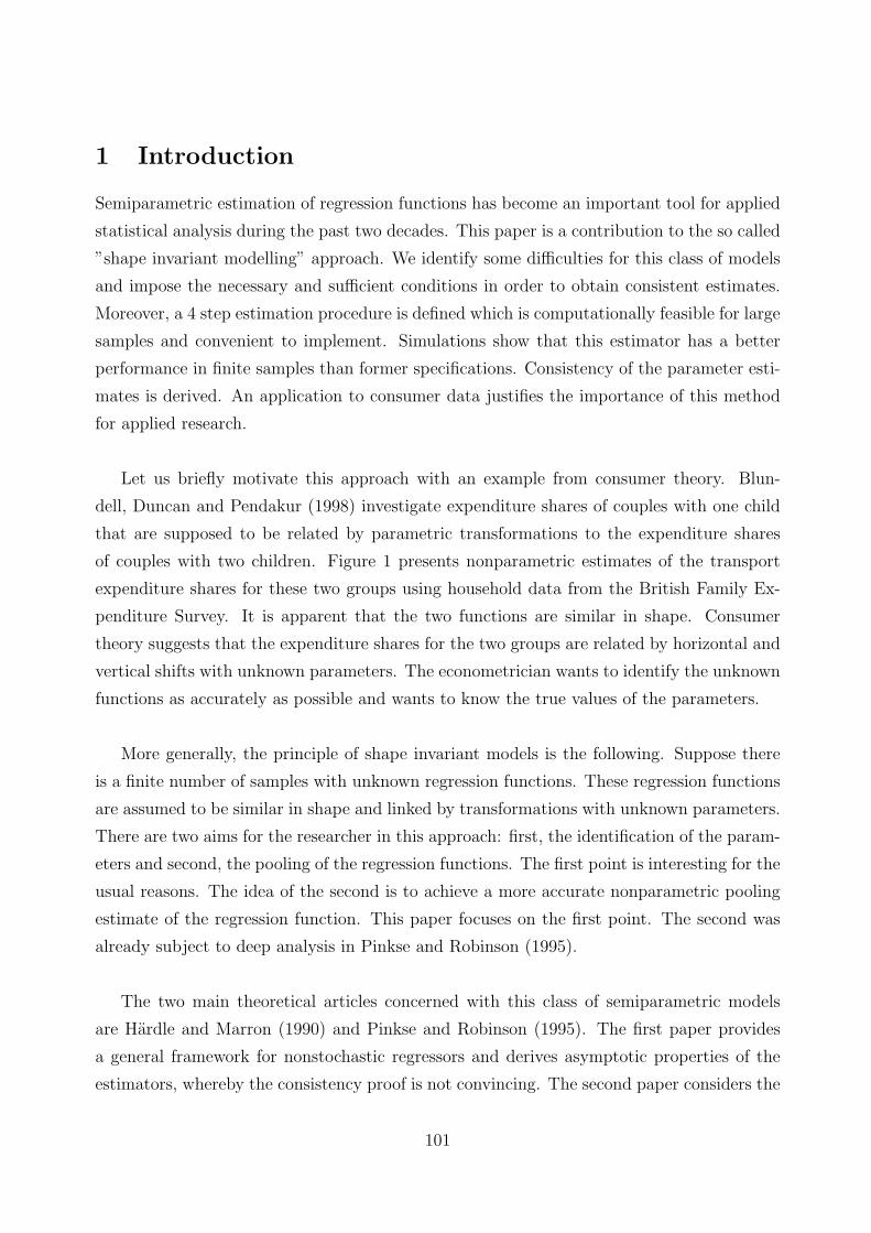
1 Introduction
Semiparametric estimation of regression functions has become an important tool for applied
statistical analysis during the past two decades. This paper is a contribution to the so called
”shape invariant modelling” approach. We identify some difficulties for this class of models
and impose the necessary and sufficient conditions in order to obtain consistent estimates.
Moreover, a 4 step estimation procedure is defined which is computationally feasible for large
samples and convenient to implement. Simulations show that this estimator has a better
performance in finite samples than former specifications. Consistency of the parameter esti-
mates is derived. An application to consumer data justifies the importance of this method
for applied research.
Let us briefly motivate this approach with an example from consumer theory. Blun-
dell, Duncan and Pendakur (1998) investigate expenditure shares of couples with one child
that are supposed to be related by parametric transformations to the expenditure shares
of couples with two children. Figure 1 presents nonparametric estimates of the transport
expenditure shares for these two groups using household data from the British Family Ex-
penditure Survey. It is apparent that the two functions are similar in shape. Consumer
theory suggests that the expenditure shares for the two groups are related by horizontal and
vertical shifts with unknown parameters. The econometrician wants to identify the unknown
functions as accurately as possible and wants to know the true values of the parameters.
More generally, the principle of shape invariant models is the following. Suppose there
is a finite number of samples with unknown regression functions. These regression functions
are assumed to be similar in shape and linked by transformations with unknown parameters.
There are two aims for the researcher in this approach: first, the identification of the param-
eters and second, the pooling of the regression functions. The first point is interesting for the
usual reasons. The idea of the second is to achieve a more accurate nonparametric pooling
estimate of the regression function. This paper focuses on the first point. The second was
already subject to deep analysis in Pinkse and Robinson (1995).
The two main theoretical articles concerned with this class of semiparametric models
are Hardle and Marron (1990) and Pinkse and Robinson (1995). The first paper provides
a general framework for nonstochastic regressors and derives asymptotic properties of the
estimators, whereby the consistency proof is not convincing. The second paper considers the
101
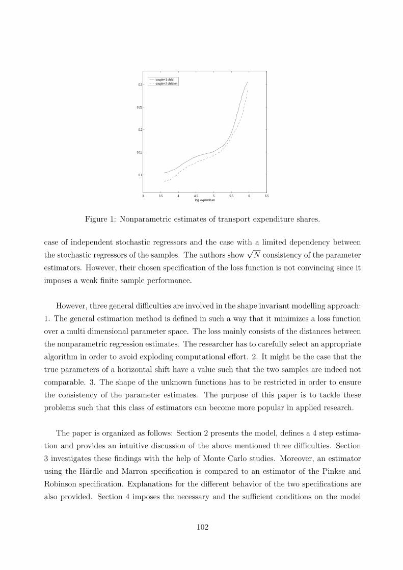
3 3.5 4 4.5 5 5.5 6 6.5
0.1
0.15
0.2
0.25
0.3
log. expenditure
couple+1 child couple+2 children
Figure 1: Nonparametric estimates of transport expenditure shares.
case of independent stochastic regressors and the case with a limited dependency between
the stochastic regressors of the samples. The authors show√
N consistency of the parameter
estimators. However, their chosen specification of the loss function is not convincing since it
imposes a weak finite sample performance.
However, three general difficulties are involved in the shape invariant modelling approach:
1. The general estimation method is defined in such a way that it minimizes a loss function
over a multi dimensional parameter space. The loss mainly consists of the distances between
the nonparametric regression estimates. The researcher has to carefully select an appropriate
algorithm in order to avoid exploding computational effort. 2. It might be the case that the
true parameters of a horizontal shift have a value such that the two samples are indeed not
comparable. 3. The shape of the unknown functions has to be restricted in order to ensure
the consistency of the parameter estimates. The purpose of this paper is to tackle these
problems such that this class of estimators can become more popular in applied research.
The paper is organized as follows: Section 2 presents the model, defines a 4 step estima-
tion and provides an intuitive discussion of the above mentioned three difficulties. Section
3 investigates these findings with the help of Monte Carlo studies. Moreover, an estimator
using the Hardle and Marron specification is compared to an estimator of the Pinkse and
Robinson specification. Explanations for the different behavior of the two specifications are
also provided. Section 4 imposes the necessary and the sufficient conditions on the model
102

such that the parameter estimates are indeed consistent. Section 5 presents an application
to consumer data.
2 The Model
Consider two samples (Yi, Xi)i=1,...,N and (Zi,Wi)i=1,...,N of size N . The sample sizes might
also be different without affecting the following analysis. Suppose
Yi = m0(Xi) + Ui
Zi = m1(Wi) + Vi, i = 1, . . . , N
with E[Ui|Xj] = E[Vi|Wj] = 0 almost surely for all i, j. Ui and Vi have finite second moments
and the pairs (Ui, Vi) are mutually independent. Xi ∈ X1 and Wi ∈ W are random variables
with i.i.d realizations on compact sets with continuous marginal distributions infx∈X1fx(x) >
0 and infw∈Wfw(w) > 0. Suppose the unknown functions m0 and m1 are twice differentiable.
Let m0 and m1 and its first two derivatives be uniformly continuous and bounded over their
supports. Furthermore a0, b0 and µ0 are unknown parameters in the interior of open subsets
in IR. The following equation is supposed to hold:
m1(x) = a0 + b0m0
(Tµ0(x)
), (1)
where T is an invertible parametric transformation with T−1µ0
(Wi) ∈ X2 and Tµ(Xi) ∈ Wµ.
In other words there exist parametric links with unknown parameters between the unknown
functions m0 and m1. Let us denote m1(x) and mµ(x) = m0(Tµ(x)) the nonparametric
estimates of m1(x) and mµ(x) = m0(Tµ(x)) respectively. This model setup is similar to one
of the models defined in Pinkse and Robinson (1995).
Since we intent to analyze a problem with a simple structure, we suppose in the following
Tµ(x) = Tc(x) = x − c. Model (1) now becomes:
m1(x) = a0 + b0m0(x − c0), (2)
where c0 ∈ C ⊂ IR. Accordingly, let denote Wc = Wµ and mc(x) = m0(x − c).
Pinkse and Robinson (1995) The definition of this estimator is essentially based on the
Nadaraya-Watson estimator. Define:
m1(x) = r(x)/f(x) and
mc(x) = rc(x)/fc(x),
103
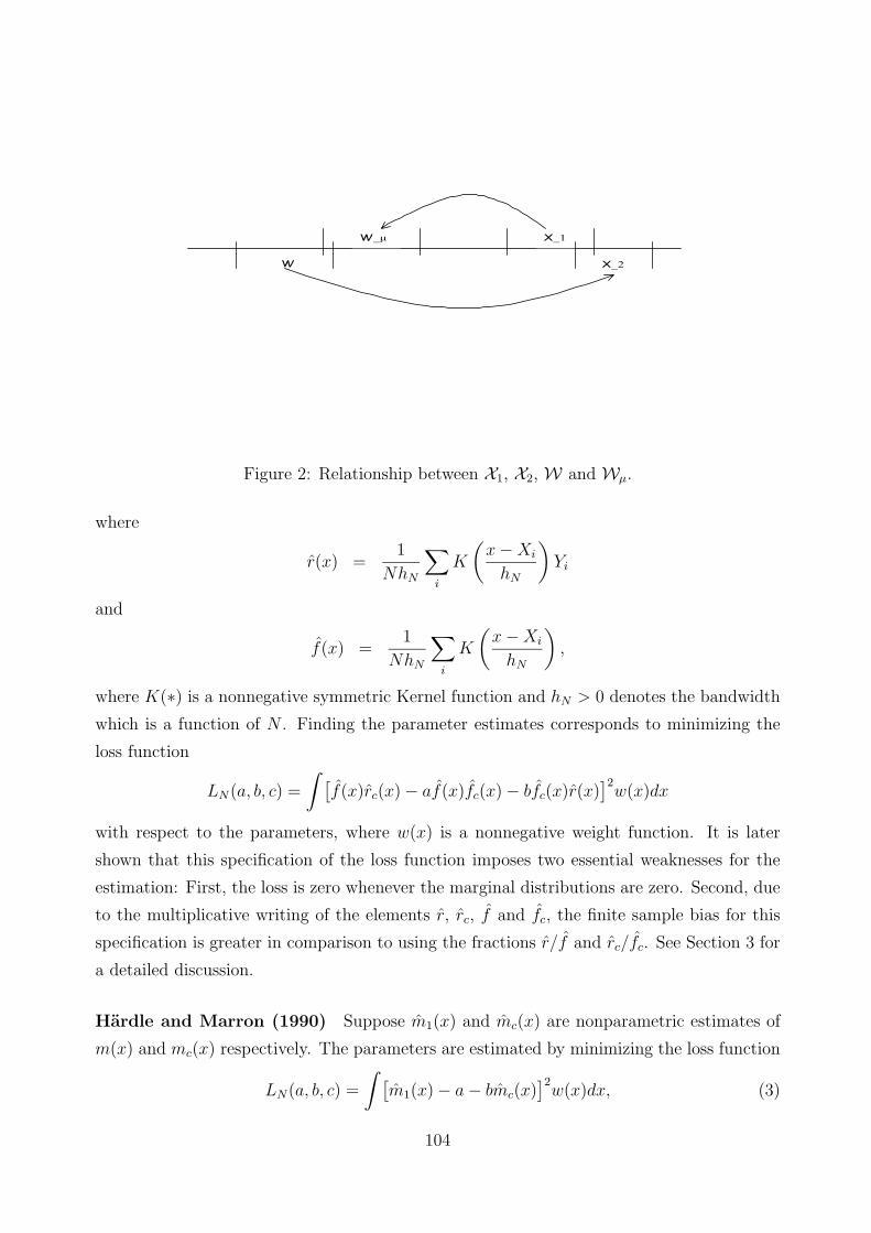
W
X_1
X_2
W_µ
Figure 2: Relationship between X1, X2, W and Wµ.
where
r(x) =1
NhN
∑i
K
(x − Xi
hN
)Yi
and
f(x) =1
NhN
∑i
K
(x − Xi
hN
),
where K(∗) is a nonnegative symmetric Kernel function and hN > 0 denotes the bandwidth
which is a function of N . Finding the parameter estimates corresponds to minimizing the
loss function
LN(a, b, c) =
∫ [f(x)rc(x) − af(x)fc(x) − bfc(x)r(x)
]2w(x)dx
with respect to the parameters, where w(x) is a nonnegative weight function. It is later
shown that this specification of the loss function imposes two essential weaknesses for the
estimation: First, the loss is zero whenever the marginal distributions are zero. Second, due
to the multiplicative writing of the elements r, rc, f and fc, the finite sample bias for this
specification is greater in comparison to using the fractions r/f and rc/fc. See Section 3 for
a detailed discussion.
Hardle and Marron (1990) Suppose m1(x) and mc(x) are nonparametric estimates of
m(x) and mc(x) respectively. The parameters are estimated by minimizing the loss function
LN(a, b, c) =
∫ [m1(x) − a − bmc(x)
]2w(x)dx, (3)
104
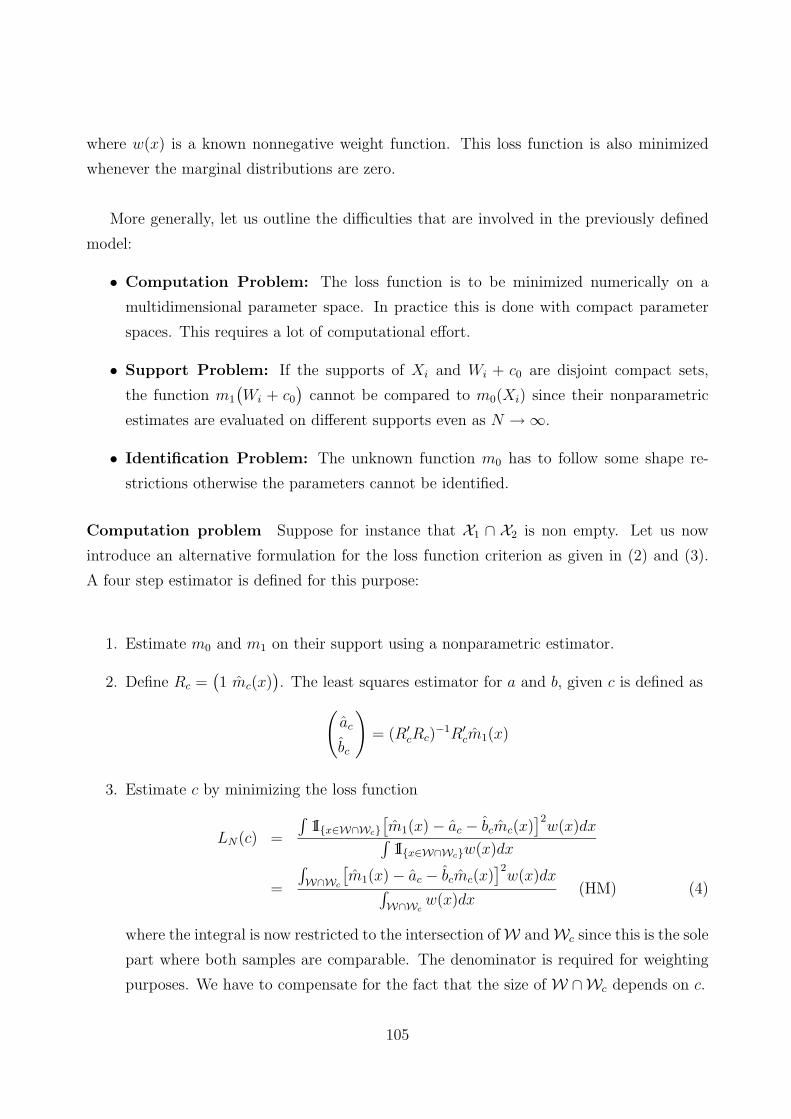
where w(x) is a known nonnegative weight function. This loss function is also minimized
whenever the marginal distributions are zero.
More generally, let us outline the difficulties that are involved in the previously defined
model:
• Computation Problem: The loss function is to be minimized numerically on a
multidimensional parameter space. In practice this is done with compact parameter
spaces. This requires a lot of computational effort.
• Support Problem: If the supports of Xi and Wi + c0 are disjoint compact sets,
the function m1
(Wi + c0
)cannot be compared to m0(Xi) since their nonparametric
estimates are evaluated on different supports even as N → ∞.
• Identification Problem: The unknown function m0 has to follow some shape re-
strictions otherwise the parameters cannot be identified.
Computation problem Suppose for instance that X1 ∩ X2 is non empty. Let us now
introduce an alternative formulation for the loss function criterion as given in (2) and (3).
A four step estimator is defined for this purpose:
1. Estimate m0 and m1 on their support using a nonparametric estimator.
2. Define Rc =(1 mc(x)
). The least squares estimator for a and b, given c is defined as
(ac
bc
)= (R′
cRc)−1R′
cm1(x)
3. Estimate c by minimizing the loss function
LN(c) =
∫1I{x∈W∩Wc}
[m1(x) − ac − bcmc(x)
]2w(x)dx∫
1I{x∈W∩Wc}w(x)dx
=
∫W∩Wc
[m1(x) − ac − bcmc(x)
]2w(x)dx∫
W∩Wcw(x)dx
(HM) (4)
where the integral is now restricted to the intersection of W and Wc since this is the sole
part where both samples are comparable. The denominator is required for weighting
purposes. We have to compensate for the fact that the size of W ∩Wc depends on c.
105
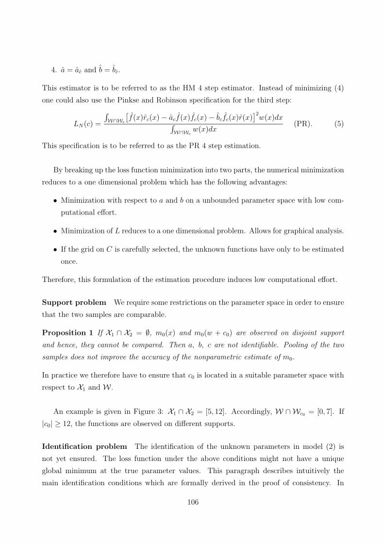
4. a = ac and b = bc.
This estimator is to be referred to as the HM 4 step estimator. Instead of minimizing (4)
one could also use the Pinkse and Robinson specification for the third step:
LN(c) =
∫W∩Wc
[f(x)rc(x) − acf(x)fc(x) − bcfc(x)r(x)
]2w(x)dx∫
W∩Wcw(x)dx
(PR). (5)
This specification is to be referred to as the PR 4 step estimation.
By breaking up the loss function minimization into two parts, the numerical minimization
reduces to a one dimensional problem which has the following advantages:
• Minimization with respect to a and b on a unbounded parameter space with low com-
putational effort.
• Minimization of L reduces to a one dimensional problem. Allows for graphical analysis.
• If the grid on C is carefully selected, the unknown functions have only to be estimated
once.
Therefore, this formulation of the estimation procedure induces low computational effort.
Support problem We require some restrictions on the parameter space in order to ensure
that the two samples are comparable.
Proposition 1 If X1 ∩ X2 = ∅, m0(x) and m0(w + c0) are observed on disjoint support
and hence, they cannot be compared. Then a, b, c are not identifiable. Pooling of the two
samples does not improve the accuracy of the nonparametric estimate of m0.
In practice we therefore have to ensure that c0 is located in a suitable parameter space with
respect to X1 and W .
An example is given in Figure 3: X1 ∩ X2 = [5, 12]. Accordingly, W ∩ Wc0 = [0, 7]. If
|c0| ≥ 12, the functions are observed on different supports.
Identification problem The identification of the unknown parameters in model (2) is
not yet ensured. The loss function under the above conditions might not have a unique
global minimum at the true parameter values. This paragraph describes intuitively the
main identification conditions which are formally derived in the proof of consistency. In
106

0 2 4 6 8 10 12 14 16 18−1
−0.5
0
0.5
1
1.5
2
2.5
3
x,w
m0(x)
2+m0(w+5)
Figure 3: Intersection of observed support: y = sin(0.5x), z = 2 + sin(0.5(w + 5)
), X1 =
[0, 12], W = [0, 12] and X2 = [5, 17].
particular, we have to impose some shape restrictions for the unknown function m0. These
conditions are violated if:
1. The unknown function m0(x) belongs to the class of linear functions.
2. The unknown function m0(x) is cycling, i.e.
∃c ∈ C such that for all x − c ∈ W ∩Wc, m0(x) = m0(x − c).
The first difficulty makes it impossible to identify a and c. The loss functions (4) and (5)
are constant in this case, i.e. L(c) = L:
Proposition 2 If m0(x) belongs to the class of linear functions, L(c) is constant and there-
fore does not posses a local minimum since the sufficient condition ∂2c L(c) > 0 does not hold.
The parameters a and c cannot be identified. Nevertheless, a pooling estimate might yield a
more accurate estimate of the unknown function.
The second difficulty implies that (4) and (5) do not have a unique minimum on the support
of c, but there is a multiple set of global minima. Therefore c cannot be identified.
Proposition 3 If m0 is cycling on W ∩Wc, the parameter c cannot be identified.
Figure 4 presents an example using a cycling sine function. In this case there are three
minima of the loss function on C.
107

−10 −8 −6 −4 −2 0 2 4 6 8 100
5
10
15
20
25
30
Figure 4: Multiple minima of the loss function: y = sin(0.5x), z = 5 + 0.5sin(0.5(x − c)),
C = [−10, 10], c0 = 0.5.
However, the smaller is the intersection of X1 and X2, the more unlikely the non-linearity
condition holds because we have imposed some smoothness conditions on the unknown func-
tions. This might lead to the following complication: The nonlinear parts of mc0(x) drop
out of the support and a and c are not longer identifiable.
Proposition 4 If the intersection of X1 and X2 is too small, the identification of the pa-
rameters might be impossible even as N → ∞.
This difficulty should have relevance in applications. It is therefore reasonable to restrict C
such that the intersection of W and Wc is not too small. However, even if the parameters
are identifiable, the convergence rate of the parametric estimator is lower than√
N since
many of the observations cannot be used for the estimation.
3 Simulations
Let us now investigate the finite sample performance of the 4 step estimator defined above
using the HM specification as given in (4) and the PR specification as given in (5). Moreover,
the semiparametric estimators are compared to a parametric estimator. It turns out that
the results for the two semiparametric estimators differ. Explanations for these differences
are provided afterwards.
108

HM4SE PR4SE HM4SE PR4SE
a 5.2328(1.2211) 6.8020(6.7376) 4.8844(0.3122) 4.1837(4.0385)
b 2.1716(7.9016) -0.4570(31.2005) 0.2633(10.4807) -1.1374(19.3405)
c 0.2398(2.2289) 0.4324(12.6926) 0.9527(10.5263) -1.6030(12.8688)
Table 1: Mean parameter estimates of the first (left) and of the second (right) Monte Carlo
experiment; (variances in brackets)
Let λ denote the Lebesgue measure defined on the smallest σ-algebra containing all open
sets in IR. For simplicity suppose λ(X1) = λ(W) in this section. Suppose also X1 = W and
λ(X1 ∩ X2) ≥ λ(X1)/2. The latter condition implies c ∈ [−λ(X1), λ(X1)]. As a consequence
of Proposition 4 we restrict C such that c ∈ [−λ(X1)/2, λ(X1)/2]. Therefore, C is properly
defined.
Monte Carlo Study Two Monte Carlo series shall help to investigate the properties of
both estimators. The following model is used:
m1(x) = 5 + 3sin(0.5(x − c0)
)m0(x) = sin(0.5x),
Xi,Wi ∼ U(0, 10), Ui, Vi ∼ N(0, 1), N = 200, 1000 simulations. The two experiments only
differ due to the value of c0, where we use c0 = 0 in the first Monte Carlo study and c0 = 4
in the second. The model setup up is interesting because the estimators have to detect a
unique minimum of the loss function in the first experiment and two minima in the second
experiment.
Figure 5 and 6 show the mean loss functions in c for the parametric estimator, the HM
4 step estimator and the PR 4 step estimator. Note that the loss functions have different
scalings and can therefore only compared in relative shape. Table 1 presents the mean pa-
rameter estimates of the two experiments.
The results of the simulations can be summarized as follows. The HM 4 step estimator
detects any minimum of the loss functions. This is in contrast to the PR 4 step estimator
which performs badly in the second experiment since it does not detect one of the minima.
Moreover, from Table 1 it is apparent that the HM 4 step estimator is superior to the PR 4
step estimator under the imposed model specification.
109

−5 0 50
0.002
0.004
0.006
0.008
0.01
0.012
0.014
0.016OLS
c−5 0 5
0
0.1
0.2
0.3
0.4
0.5
0.6
0.7
0.8
0.9
1HM4SE
c−5 0 5
0.4
0.6
0.8
1
1.2
1.4
1.6
1.8x 10
−4 PR4SE
c
Figure 5: Mean conditional Loss functions L(c|a, b) of the first Monte Carlo Series (c0 = 0):
a) parametric b)HM 4 step estimator c) PR 4 step estimator.
−5 0 52
4
6
8
10
12
14x 10
−3 OLS
c−5 0 5
0
0.05
0.1
0.15
0.2
0.25
0.3
0.35
0.4
0.45
0.5HM4SE
c−5 0 5
0.2
0.4
0.6
0.8
1
1.2
1.4
1.6
1.8
2x 10
−4 PR4SE
c
Figure 6: Mean conditional Loss functions L(c|a, b) of the second Monte Carlo Series (c0 = 4):
a) parametric b)HM 4 step estimator c) PR 4 step estimator.
110
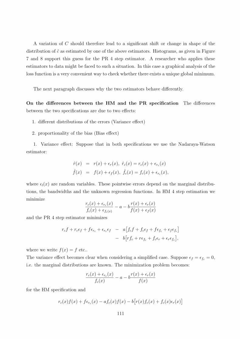
A variation of C should therefore lead to a significant shift or change in shape of the
distribution of c as estimated by one of the above estimators. Histograms, as given in Figure
7 and 8 support this guess for the PR 4 step estimator. A researcher who applies these
estimators to data might be faced to such a situation. In this case a graphical analysis of the
loss function is a very convenient way to check whether there exists a unique global minimum.
The next paragraph discusses why the two estimators behave differently.
On the differences between the HM and the PR specification The differences
between the two specifications are due to two effects:
1. different distributions of the errors (Variance effect)
2. proportionality of the bias (Bias effect)
1. Variance effect: Suppose that in both specifications we use the Nadaraya-Watson
estimator:
r(x) = r(x) + εr(x), rc(x) = rc(x) + εrc(x)
f(x) = f(x) + εf (x), fc(x) = fc(x) + εrc(x),
where εl(x) are random variables. These pointwise errors depend on the marginal distribu-
tions, the bandwidths and the unknown regression functions. In HM 4 step estimation we
minimizerc(x) + εrc(x)
fc(x) + εfc(x)
− a − br(x) + εr(x)
f(x) + εf (x)
and the PR 4 step estimator minimizes
rcf + rcεf + fεrc + εrcεf − a[fcf + fcεf + fεfc + εfεfc
]− b
[rfc + rεfc + fcεr + εrεfc
],
where we write f(x) = f etc..
The variance effect becomes clear when considering a simplified case. Suppose εf = εfc = 0,
i.e. the marginal distributions are known. The minimization problem becomes:
rc(x) + εrc(x)
fc(x)− a − b
r(x) + εr(x)
f(x)
for the HM specification and
rc(x)f(x) + fεrc(x) − afc(x)f(x) − b[r(x)fc(x) + fc(x)εr(x)
]111
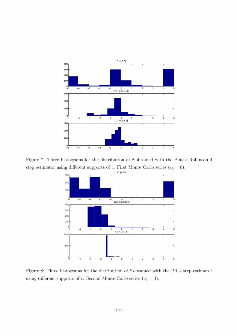
−5 −4 −3 −2 −1 0 1 2 3 4 50
100
200
300
400C=[−5,5]
−5 −4 −3 −2 −1 0 1 2 3 4 50
200
400
600C=[−3.28,3.28]
−5 −4 −3 −2 −1 0 1 2 3 4 50
100
200
300C=[−1.5,1.5]
Figure 7: Three histograms for the distribution of c obtained with the Pinkse-Robinson 4
step estimator using different supports of c. First Monte Carlo series (c0 = 0).
−5 −4 −3 −2 −1 0 1 2 3 4 50
100
200
300C=[−5,5]
−5 −4 −3 −2 −1 0 1 2 3 4 50
100
200
300
400C=[−3.28,3.28]
−5 −4 −3 −2 −1 0 1 2 3 4 50
500
1000C=[−1.5,1.5]
Figure 8: Three histograms for the distribution of c obtained with the PR 4 step estimator
using different supports of c. Second Monte Carlo series (c0 = 4).
112
for the PR specification. It is clear that if fc(x) = f(x), both estimators are the same. Oth-
erwise it is important to point out that their error distributions differ. The variance of the
HM 4 step estimator is larger whenever fc and f are smaller than one. Otherwise it is smaller.
2. Bias effect: The second point becomes clear when rewriting the problem:
r(x) = r(x)ξr(x), rc(x) = rc(x)ξrc(x)
f(x) = f(x)ξf (x), fc(x) = fc(x)ξrc(x)
and for the HM specification we obtain accordingly
rc(x)ξrc(x)
fc(x)ξfc(x)− a − b
r(x)ξr(x)
f(x)ξf (x).
ξr(x) and ξf (x) are unequal to one whenever the corresponding estimates are biased. From
Figure 9 it is moreover apparent that ξf (x) and ξr(x) are very similar functions. Therefore,
their ratio deviates less from one than each of the functions itself. A part of the pointwise bias
is therefore ruled out by the division. Rewriting the estimator in the Pinkse and Robinson
style causes a loss of this nice property. Estimators using the specification
f(x)ξf (x)rc(x) − afc(x)ξfc(x)f(x)ξf (x) − br(x)ξr(x)fc(x)ξfc(x)
therefore behave worse in the case of small samples in particularly at the boundaries where
the bias is supposed to be large. This effect becomes stronger due to the multiplicative
structure. As a consequence the estimates are more affected by the bias of f , fc, r and rc.
We conclude that there is a trade-off between, and which estimator is preferable depends
on the specific situation. In small samples the second point should clearly dominate the
first, since the systematic bias is more evident. The PR specification should therefore not
be applied in such cases. The simulations (N = 200) impressively support these findings.
In the second experiment (c0 = 4) the overlapping support at c0 = 4 is small. Since the
two nonparametric estimates are assumed to be more biased at the boundaries, we expect
the same for the estimates of the unknown functions on a large subset of W ∩ Wc0 . As a
consequence of the above findings, the estimator using the PR specification is not able to
detect the second minimum of the loss function (Figure 6c).
113

0 2 4 60.5
0.6
0.7
0.8
0.9
1
1.1
1.2
1.3
1.4
x
ξf(x)
ξr(x)
ξr(x)/ξ
f(x)
0 2 4 63
3.5
4
4.5
5
5.5
6
6.5
7
7.5
8
x
r(x)/f(x)estimate
Figure 9: Proportionality of the bias: N = 2000, y = 3 + 5sin(0.5x), x ∼ U [0, 6], h = 0.5,
mean of 1000 samples
4 Asymptotic Properties
This section derives asymptotic properties for the model defined in Section 2. For this
purpose we use a modified Hardle and Marron loss function as given in (3) that incorporates
the intuitive findings of Section 2.
Consistency Hardle and Marron (1990) assume that the loss function is convex around
the true parameter values. We are going to derive here the necessary and sufficient con-
ditions on the shape of the unknown function m0 such that the loss function indeed has a
unique minimum.
Denote by m(x) the nonparametric estimate of m0 evaluated at Xi = x. Accordingly, we
have x − c ∈ Wc for all c ∈ C. Let be {xt − c} = {x − c|x − c ∈ W} for all c ∈ C. Define
Tc = card{x − c|x − c ∈ W}. Note that Tc ≤ N and Tc weakly increases in N .
Assumption 1 c0 is an interior point of C, where C is such that for all c ∈ C: Tc ≥ 3.
Tc > 0 solves the support problem. Tc ≥ 3 is required for the identifiability of a,
b and c. Define a sequence t = 1, . . . , Tc of evaluation points wct ∈ W such that for a
given c: {wct}t=1,...,Tc = {xt − c}t=1,...,Tc . Denote {m1(w
ct )}t=1,...,Tc = {m1(xt − c0)}t=1,...,Tc
as the nonparametric estimates of m1 evaluated at wct . Moreover, denote m0(x − c) as the
114

nonparametric estimate of m0 evaluated at x and horizontally shifted to x − c for all x and
c. The loss function (4) can then be rewritten as:
LN(a, b, c) =Tc∑t=1
[m1(xt − c0) − a − bm0(xt − c)
]2/Tc. (6)
Intuitively, the loss per evaluation point is minimized. Note that this function depends on
N due to the nonparametric estimates and Tc. The following two assumption are necessary
for the identifiability and have already been discussed in Section 2.
Assumption 2 m0(xt − c) is not cycling on W ∩Wc, i.e. there does not exists c = c0 such
that m0(xt − c) = m0(xt − c0) for all xt − c ∈ W ∩Wc.
Assumption 3 m0(xt − c) is nonlinear on W ∩Wc for all c, i.e.
(1 m(xt − c) m′(xt − c))
are linearly independent on W ∩Wc for all c.
Assumptions 1-3 ensure the necessary conditions for the consistency of the parameter esti-
mates.
The nonparametric estimates for m0 and m1 can be written as
m1(xt − c0) = a0 + b0m0(xt − c0) + ε1(wct , N) (7)
m0(xt − c) = m0(xt − c) + ε0(xt − c,N). (8)
for t = 1, . . . , Tc given c ∈ C.
Assumption 4 ε0(x,N) and ε1(w,N) converge to 0 in probability uniformly in x and w,
i.e.
limN→∞P[supx∈X1
|ε0(x,N)| < δ]
= 1 for any δ > 0
limN→∞P[supw∈W |ε1(w,N)| < δ
]= 1 for any δ > 0.
This assumption can be for example justified for the class of Kernel estimators by the fol-
lowing theorem:
115
Theorem 2.1 Nadaraya (1989), p.122 The Kernel estimators of the regression func-
tions are uniformly strongly consistent, i.e.
supx∈X1|m0(x) − m0(x)| → 0 a.s.
supw∈W |m1(w) − m1(w)| → 0 a.s.
if the following conditions on the bandwidth and on the Kernel function hold:
0 < hN → 0 as N → ∞ and
∞∑N=1
exp(−γNh2N) < ∞ for any γ > 0.
K(x) is a kernel function which satisfies:
sup−∞<x<∞∣∣K(x)
∣∣ < ∞lim|x|→∞
∣∣x∣∣K(x) = 0
K(x) = K(−x)
x2K(x)dx ∈ L1(−∞,∞)
K(x) is a function with bounded variation on X1 and W .
However, there is a broad class of nonparametric estimators satisfying Assumption 4, e.g.
local polynomials and splines.
Let us now state the theorem of this paragraph which says that the parameter estimates
a, b and c are weakly consistent under appropriate regularity conditions:
Theorem 1 Under assumptions 1-4, a root of Model (6) is consistent, i.e.
limN→∞P
infa,b,c∈B
a
b
c
−
a0
b0
c0
′
a
b
c
−
a0
b0
c0
> ε
= 0 for any ε > 0
where B is the set of roots. Moreover, the set of roots consists of one single element.
Proof: Appendix 1.
Asymptotic Normality Asymptotic normality has already been shown by Hardle and
Marron (1990) and Pinkse and Robinson (1995) for their frameworks. Both show that despite
the lower convergence rate of the nonparametric estimates, the rate√
N for the parametric
116
estimates can be achieved. Whether it is indeed achieved mainly depends on the convergence
rate of the nonparametric estimator.
Using the loss function specification as given in (6), this does not hold in general since
Tc ≤ N . If X1 and X2 are small enough then Tc0 tends to be much smaller than N as
N becomes large. In this case it is hard to believe that the parameter estimates converge
at rate√
N since the number of observations that count for the comparison of the two
samples is much smaller. It is therefore more reasonable that the convergence rate of the
parameters depends on the probability that the event Xi − c0 ∈ W and Wi ∈ Wc0 occurs.
This probability depends on the proportion of each marginal distribution that is assigned to
W ∩Wc0 : ∫W∩Wc0
fj(x)dx, j = x,w,
where Xi and Wi are independent. A later version of this paper will present more details in
form of a simulation study and in form of a theorem.
Note that Pinkse and Robinson and Hardle and Marron specify their loss functions in
such a way that it takes into account N realizations and not only the observations in W∩Wc.
5 Application
This section is devoted to an application of the HM 4 step estimator to consumer data. We
mainly follow Blundell, Duncan and Pendakur (1998) who use an estimator of the Pinkse
and Robinson specification in order to estimate unknown expenditure shares under shape
invariance restrictions. It should therefore be of interest to investigate how the HM 4 step
estimator behaves in comparison. We use the same cross section samples of the British
Family Expenditure Survey (FES I) for this purpose. Afterwards the estimation is done for
samples (FES II) which are also used in Blundell, Chen and Kristensen (2001).
Blundell, Duncan and Pendakur estimate expenditure shares for several commodities
using an extended semiparametric specification as given in the model of Section 2. The
parametric shifts are now related to observable household characteristics like the number of
children in a household. Accordingly, they compare couples with one child to couples with
two children. The expenditure shares for the two groups are linked by the following model:
m1(x) = a + m0(x − c),
117
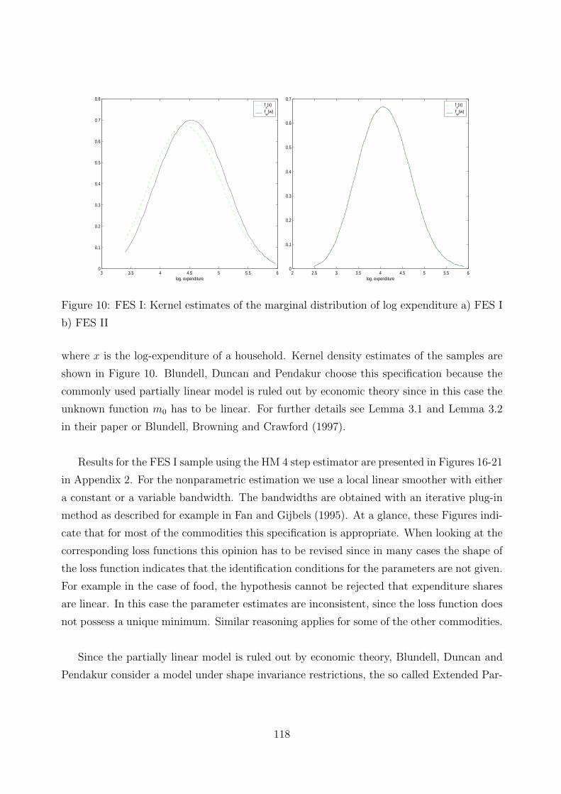
3 3.5 4 4.5 5 5.5 60
0.1
0.2
0.3
0.4
0.5
0.6
0.7
0.8
log. expenditure
fx(x)
fw
(w)
2 2.5 3 3.5 4 4.5 5 5.5 60
0.1
0.2
0.3
0.4
0.5
0.6
0.7
log. expenditure
fx(x)
fw
(w)
Figure 10: FES I: Kernel estimates of the marginal distribution of log expenditure a) FES I
b) FES II
where x is the log-expenditure of a household. Kernel density estimates of the samples are
shown in Figure 10. Blundell, Duncan and Pendakur choose this specification because the
commonly used partially linear model is ruled out by economic theory since in this case the
unknown function m0 has to be linear. For further details see Lemma 3.1 and Lemma 3.2
in their paper or Blundell, Browning and Crawford (1997).
Results for the FES I sample using the HM 4 step estimator are presented in Figures 16-21
in Appendix 2. For the nonparametric estimation we use a local linear smoother with either
a constant or a variable bandwidth. The bandwidths are obtained with an iterative plug-in
method as described for example in Fan and Gijbels (1995). At a glance, these Figures indi-
cate that for most of the commodities this specification is appropriate. When looking at the
corresponding loss functions this opinion has to be revised since in many cases the shape of
the loss function indicates that the identification conditions for the parameters are not given.
For example in the case of food, the hypothesis cannot be rejected that expenditure shares
are linear. In this case the parameter estimates are inconsistent, since the loss function does
not possess a unique minimum. Similar reasoning applies for some of the other commodities.
Since the partially linear model is ruled out by economic theory, Blundell, Duncan and
Pendakur consider a model under shape invariance restrictions, the so called Extended Par-
118
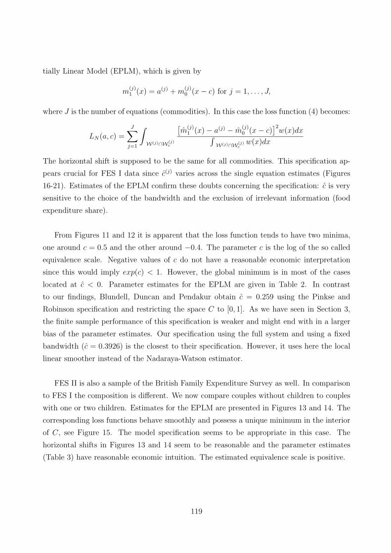
tially Linear Model (EPLM), which is given by
m(j)1 (x) = a(j) + m
(j)0 (x − c) for j = 1, . . . , J,
where J is the number of equations (commodities). In this case the loss function (4) becomes:
LN(a, c) =J∑
j=1
∫W(j)∩W(j)
c
[m
(j)1 (x) − a(j) − m
(j)0 (x − c)
]2w(x)dx∫
W(j)∩W(j)c
w(x)dx
The horizontal shift is supposed to be the same for all commodities. This specification ap-
pears crucial for FES I data since c(j) varies across the single equation estimates (Figures
16-21). Estimates of the EPLM confirm these doubts concerning the specification: c is very
sensitive to the choice of the bandwidth and the exclusion of irrelevant information (food
expenditure share).
From Figures 11 and 12 it is apparent that the loss function tends to have two minima,
one around c = 0.5 and the other around −0.4. The parameter c is the log of the so called
equivalence scale. Negative values of c do not have a reasonable economic interpretation
since this would imply exp(c) < 1. However, the global minimum is in most of the cases
located at c < 0. Parameter estimates for the EPLM are given in Table 2. In contrast
to our findings, Blundell, Duncan and Pendakur obtain c = 0.259 using the Pinkse and
Robinson specification and restricting the space C to [0, 1]. As we have seen in Section 3,
the finite sample performance of this specification is weaker and might end with in a larger
bias of the parameter estimates. Our specification using the full system and using a fixed
bandwidth (c = 0.3926) is the closest to their specification. However, it uses here the local
linear smoother instead of the Nadaraya-Watson estimator.
FES II is also a sample of the British Family Expenditure Survey as well. In comparison
to FES I the composition is different. We now compare couples without children to couples
with one or two children. Estimates for the EPLM are presented in Figures 13 and 14. The
corresponding loss functions behave smoothly and possess a unique minimum in the interior
of C, see Figure 15. The model specification seems to be appropriate in this case. The
horizontal shifts in Figures 13 and 14 seem to be reasonable and the parameter estimates
(Table 3) have reasonable economic intuition. The estimated equivalence scale is positive.
119
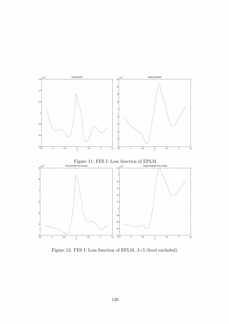
−1.5 −1 −0.5 0 0.5 1 1.50.4
0.6
0.8
1
1.2
1.4
1.6x 10
−4 fixed bandwidth
c−1.5 −1 −0.5 0 0.5 1 1.52
3
4
5
6
7
8
9
10
11x 10
−4 variable bandwidth
c
Figure 11: FES I: Loss function of EPLM
−1.5 −1 −0.5 0 0.5 1 1.53
4
5
6
7
8
9x 10
−4 fixed bandwidth, food excluded
c−1.5 −1 −0.5 0 0.5 1 1.5
0.2
0.4
0.6
0.8
1
1.2
1.4
1.6
1.8
2
2.2x 10
−3 variable bandwidth, food excluded
c
Figure 12: FES I: Loss function of EPLM, J=5 (food excluded).
120
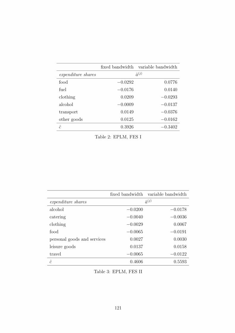
fixed bandwidth variable bandwidth
expenditure shares a(j)
food −0.0292 0.0776
fuel −0.0176 0.0140
clothing 0.0209 −0.0293
alcohol −0.0009 −0.0137
transport 0.0149 −0.0376
other goods 0.0125 −0.0162
c 0.3926 −0.3402
Table 2: EPLM, FES I
fixed bandwidth variable bandwidth
expenditure shares a(j)
alcohol −0.0200 −0.0178
catering −0.0040 −0.0036
clothing −0.0029 0.0067
food −0.0065 −0.0191
personal goods and services 0.0027 0.0030
leisure goods 0.0137 0.0158
travel −0.0065 −0.0122
c 0.4606 0.5593
Table 3: EPLM, FES II
121
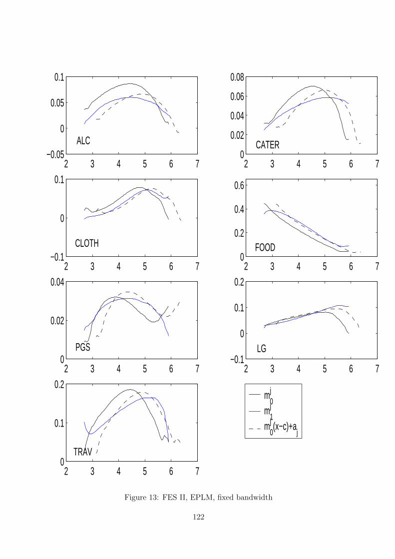
2 3 4 5 6 7−0.05
0
0.05
0.1
2 3 4 5 6 70
0.02
0.04
0.06
0.08
2 3 4 5 6 7−0.1
0
0.1
2 3 4 5 6 70
0.2
0.4
0.6
2 3 4 5 6 70
0.02
0.04
2 3 4 5 6 7−0.1
0
0.1
0.2
2 3 4 5 6 70
0.1
0.2m
0j
m1j
m0j (x−c)+a
j
ALC
CLOTH
TRAV
PGS
CATER
FOOD
LG
Figure 13: FES II, EPLM, fixed bandwidth
122
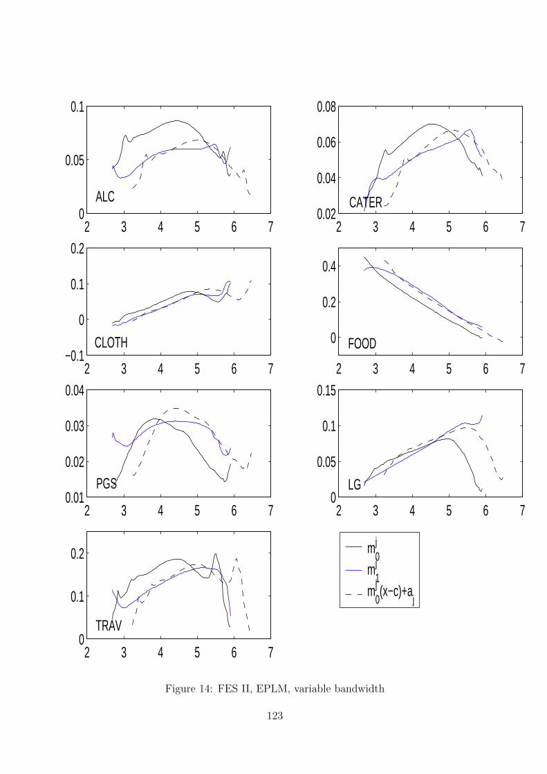
2 3 4 5 6 70
0.05
0.1
2 3 4 5 6 70.02
0.04
0.06
0.08
2 3 4 5 6 7−0.1
0
0.1
0.2
2 3 4 5 6 7
0
0.2
0.4
2 3 4 5 6 70.01
0.02
0.03
0.04
2 3 4 5 6 70
0.05
0.1
0.15
2 3 4 5 6 70
0.1
0.2 m0j
m1j
m0j (x−c)+a
j
ALC
CLOTH
PGS
TRAV
CATER
FOOD
LG
Figure 14: FES II, EPLM, variable bandwidth
123
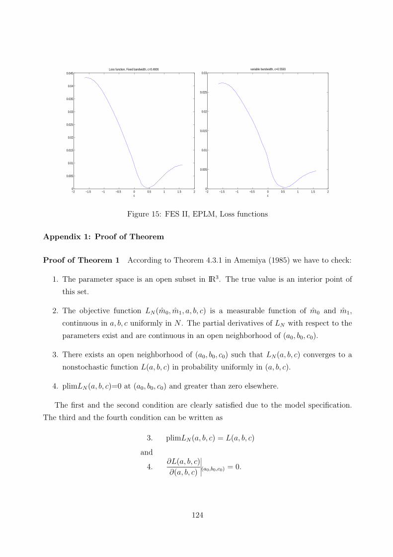
−2 −1.5 −1 −0.5 0 0.5 1 1.5 20
0.005
0.01
0.015
0.02
0.025
0.03
0.035
0.04
0.045Loss function, Fixed bandwidth, c=0.4606
c−2 −1.5 −1 −0.5 0 0.5 1 1.5 20
0.005
0.01
0.015
0.02
0.025
0.03variable bandwidth, c=0.5593
c
Figure 15: FES II, EPLM, Loss functions
Appendix 1: Proof of Theorem
Proof of Theorem 1 According to Theorem 4.3.1 in Amemiya (1985) we have to check:
1. The parameter space is an open subset in IR3. The true value is an interior point of
this set.
2. The objective function LN(m0, m1, a, b, c) is a measurable function of m0 and m1,
continuous in a, b, c uniformly in N . The partial derivatives of LN with respect to the
parameters exist and are continuous in an open neighborhood of (a0, b0, c0).
3. There exists an open neighborhood of (a0, b0, c0) such that LN(a, b, c) converges to a
nonstochastic function L(a, b, c) in probability uniformly in (a, b, c).
4. plimLN(a, b, c)=0 at (a0, b0, c0) and greater than zero elsewhere.
The first and the second condition are clearly satisfied due to the model specification.
The third and the fourth condition can be written as
3. plimLN(a, b, c) = L(a, b, c)
and
4.∂L(a, b, c)
∂(a, b, c)(a0,b0,c0) = 0.
124
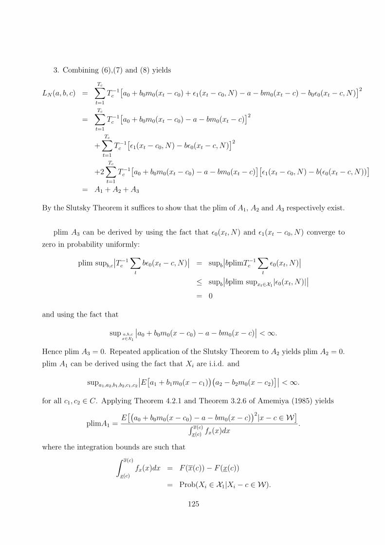
3. Combining (6),(7) and (8) yields
LN(a, b, c) =Tc∑t=1
T−1c
[a0 + b0m0(xt − c0) + ε1(xt − c0, N) − a − bm0(xt − c) − b0ε0(xt − c,N)
]2
=Tc∑t=1
T−1c
[a0 + b0m0(xt − c0) − a − bm0(xt − c)
]2
+Tc∑t=1
T−1c
[ε1(xt − c0, N) − bε0(xt − c,N)
]2
+2Tc∑t=1
T−1c
[a0 + b0m0(xt − c0) − a − bm0(xt − c)
][ε1(xt − c0, N) − b(ε0(xt − c,N))
]= A1 + A2 + A3
By the Slutsky Theorem it suffices to show that the plim of A1, A2 and A3 respectively exist.
plim A3 can be derived by using the fact that ε0(xt, N) and ε1(xt − c0, N) converge to
zero in probability uniformly:
plim supb,c
∣∣T−1c
∑t
bε0(xt − c,N)∣∣ = supb
∣∣bplimT−1c
∑t
ε0(xt, N)∣∣
≤ supb
∣∣bplim supxt∈X1|ε0(xt, N)|∣∣
= 0
and using the fact that
sup a,b,cx∈X1
∣∣a0 + b0m0(x − c0) − a − bm0(x − c)∣∣ < ∞.
Hence plim A3 = 0. Repeated application of the Slutsky Theorem to A2 yields plim A2 = 0.
plim A1 can be derived using the fact that Xi are i.i.d. and
supa1,a2,b1,b2,c1,c2
∣∣E[a1 + b1m0(x − c1)
)(a2 − b2m0(x − c2)
]∣∣ < ∞.
for all c1, c2 ∈ C. Applying Theorem 4.2.1 and Theorem 3.2.6 of Amemiya (1985) yields
plimA1 =E
[(a0 + b0m0(x − c0) − a − bm0(x − c)
)2|x − c ∈ W]∫ x(c)
x(c)fx(x)dx
.
where the integration bounds are such that∫ x(c)
x(c)
fx(x)dx = F (x(c)) − F (x(c))
= Prob(Xi ∈ X1|Xi − c ∈ W).
125

4. To be shown: The probability limit of the loss function, i.e. plimLN(a, b, c) =plimA1,
has a unique minimum at a0, b0, c0, i.e.
plim∂LN(a, b, c)
∂(a, b, c)(a0,b0,c0) = 0
We have to check the necessary and the sufficient conditions.
The first order conditions are:
∂aplimA1(a, b, c) = −2E[a0 − a + b0m0(x − c0) − bm0(x − c)|x − c ∈ W][
F (x(c)) − F (x(c))] = 0 (9)
∂bplimA1(a, b, c) = −2E[m0(x − c)
(a0 − a + b0m0(x − c0) − bm0(x − c)
)|x − c ∈ W][F (x(c)) − F (x(c))
]= 0 (10)
∂cplimA1(a, b, c) =2E
[bm′
0(x − c)(a0 − a + b0m0(x − c0) − bm0(x − c)|x − c ∈ W)][
F (x(c)) − F (x(c))]
−E[(
a0 − a + b0m0(x − c0) − bm0(x − c))2|x − c ∈ W]
[F (x(c)) − F (x(c))
]2
×[x′(c)fx(x(c)) − x′(c)fx(x(c))
](11)
= 0
From (9) and (10) we obtain
a = a0 + E[b0m0(x − c0) − bm0(x − c)|x − c ∈ W]
(12)
b =E
[m0(x − c)
(a0 − a + b0m0(x − c0)
)|x − c ∈ W]E
[m0(x − c)2|x − c ∈ W]
Substituting for a yields:
b =cov
(b0m0(x − c0),m0(x − c)|x − c ∈ W)
var (m0(x − c)|x − c ∈ W)(13)
The condition given by equation (11) is stronger than required. We need to show that the
loss function is zero at the true parameter values and greater than zero elsewhere. We know
that the denominator is greater than zero and less than or equal to one. It is therefore
enough to show that the numerator of the loss function is only zero at the true parameter
values. We can therefore substitute (11) by
2E[bm′
0(x − c)(a0 − a + b0m0(x − c0) − bm0(x − c)
)|x − c ∈ W]= 0 (14)
126
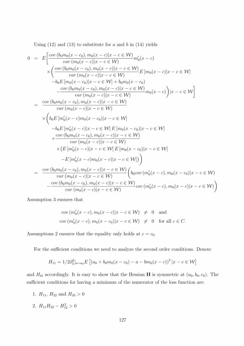
Using (12) and (13) to substitute for a and b in (14) yields
0 = E
[cov (b0m0(x − c0),m0(x − c)|x − c ∈ W)
var (m0(x − c)|x − c ∈ W)m′
0(x − c)
×(
cov (b0m0(x − c0),m0(x − c)|x − c ∈ W)
var (m0(x − c)|x − c ∈ W)E [m0(x − c)|x − c ∈ W]
−b0E [m0(x − c0)|x − c ∈ W] + b0m0(x − c0)
−cov (b0m0(x − c0),m0(x − c)|x − c ∈ W)
var (m0(x − c)|x − c ∈ W)m0(x − c)
)|x − c ∈ W
]
=cov (b0m0(x − c0),m0(x − c)|x − c ∈ W)
var (m0(x − c)|x − c ∈ W)
×(
b0E [m′0(x − c)m0(x − c0)|x − c ∈ W]
−b0E [m′0(x − c)|x − c ∈ W] E [m0(x − c0)|x − c ∈ W]
+cov (b0m0(x − c0),m0(x − c)|x − c ∈ W)
var (m0(x − c)|x − c ∈ W)
×(E [m′
0(x − c)|x − c ∈ W] E [m0(x − c0)|x − c ∈ W]
−E [m′0(x − c)m0(x − c)|x − c ∈ W]
))
=cov (b0m0(x − c0),m0(x − c)|x − c ∈ W)
var (m0(x − c)|x − c ∈ W)
(b0cov (m′
0(x − c),m0(x − c0)|x − c ∈ W)
−cov (b0m0(x − c0),m0(x − c)|x − c ∈ W)
var (m0(x − c)|x − c ∈ W)cov (m′
0(x − c),m0(x − c)|x − c ∈ W)
)
Assumption 3 ensures that
cov (m′0(x − c),m0(x − c)|x − c ∈ W) = 0 and
cov (m′0(x − c),m0(x − c0)|x − c ∈ W) = 0 for all c ∈ C.
Assumptions 2 ensures that the equality only holds at c = c0.
For the sufficient conditions we need to analyze the second order conditions. Denote
H11 = 1/2∂2a|a=a0E
[(a0 + b0m0(x − c0) − a − bm0(x − c))2 |x − c ∈ W]
and Hkl accordingly. It is easy to show that the Hessian H is symmetric at (a0, b0, c0). The
sufficient conditions for having a minimum of the numerator of the loss function are:
1. H11, H22 and H33 > 0
2. H11H22 − H212 > 0
127
3. detH > 0
The elements of the Hessian are:
H11 = 1
H22 = E[m0(x − c0)
2|x − c ∈ W]H33 = b2
0E[m′
0(x − c0)2|x − c ∈ W]
H12 = E [m0(x − c0)|x − c ∈ W]
H13 = −b0E [m′0(x − c0)|x − c ∈ W]
H23 = −b0E [m′0(x − c0)m0(x − c0)|x − c ∈ W]
Condition 1 is clearly satisfied. It is to be shown that the other two conditions also hold.
Condition 2 holds, since
E[m0(x − c0)
2|x − c ∈ W]> (E [m0(x − c0)|x − c ∈ W])2
due to the Cauchy-Schwartz inequality.
Condition 3 requires
0 < E[m0(x − c0)
2|x − c ∈ W]b20E
[m′
0(x − c0)2|x − c ∈ W]
+b20 (E [m′
0(x − c0)m0(x − c0)|x − c ∈ W])2
+E [m0(x − c0)|x − c ∈ W] b20E [m′
0(x − c0)|x − c ∈ W] E [m′0(x − c0)m0(x − c0)|x − c ∈ W]
+E [m0(x − c0)|x − c ∈ W] b20E [m′
0(x − c0)|x − c ∈ W] E [m′0(x − c0)m0(x − c0)|x − c ∈ W]
− (E [m0(x − c0)|x − c ∈ W])2 b20E
[m′
0(x − c0)2|x − c ∈ W]
−E[m0(x − c0)
2|x − c ∈ W]b20 (E [m′
0(x − c0)|x − c ∈ W])2
which is equivalent to
2 (E [m0(x − c0)|x − c ∈ W])2 (E [m′0(x − c0)|x − c ∈ W])
2
+E[m0(x − c0)
2|x − c ∈ W]E
[m′
0(x − c0)2|x − c ∈ W]
+ (E [m′0(x − c0)m0(x − c0)|x − c ∈ W])
2
> (E [m0(x − c0)|x − c ∈ W])2 E[m′
0(x − c0)2|x − c ∈ W]
+ (E [m′0(x − c0)|x − c ∈ W])
2E
[m0(x − c0)
2|x − c ∈ W].
The inequality can be shown by an application of the Cauchy- Schwarz inequality to the
second and the third term of the left hand side. �
128
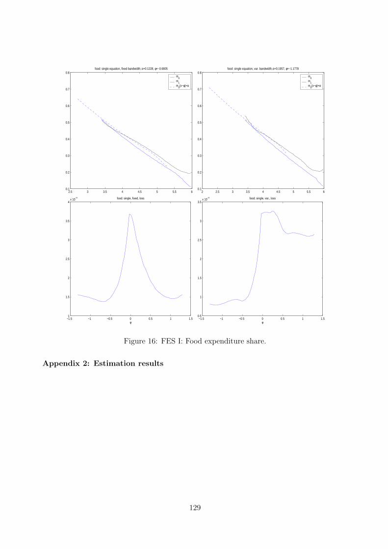
2.5 3 3.5 4 4.5 5 5.5 60.1
0.2
0.3
0.4
0.5
0.6
0.7
0.8food: single equation, fixed bandwidth, α=0.1228, φ=−0.6805
m0
m1
m0(x−φ)+α
2 2.5 3 3.5 4 4.5 5 5.5 60.1
0.2
0.3
0.4
0.5
0.6
0.7
0.8food: single equation, var. bandwidth, α=0.1957, φ=−1.1778
m0
m1
m0(x−φ)+α
−1.5 −1 −0.5 0 0.5 1 1.51
1.5
2
2.5
3
3.5
4x 10
−4 food: single, fixed, loss
φ−1.5 −1 −0.5 0 0.5 1 1.5
0.5
1
1.5
2
2.5
3
3.5x 10
−4 food: single, var., loss
φ
Figure 16: FES I: Food expenditure share.
Appendix 2: Estimation results
129
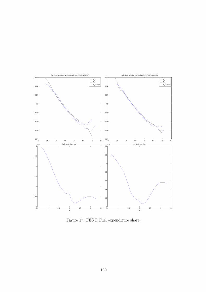
3 3.5 4 4.5 5 5.5 6 6.50.02
0.04
0.06
0.08
0.1
0.12
0.14
0.16fuel: single equation, fixed bandwidth, α=−0.0118, φ=0.2617
m0
m1
m0(x−φ)+α
3 3.5 4 4.5 5 5.5 6 6.50.02
0.04
0.06
0.08
0.1
0.12
0.14
0.16fuel: single equation, var. bandwidth, α=−0.0078, φ=0.1570
m0
m1
m0(x−φ)+α
−1.5 −1 −0.5 0 0.5 1 1.50
0.5
1
1.5
2
2.5
3x 10
−4 fuel: single, fixed, loss
φ−1.5 −1 −0.5 0 0.5 1 1.50
0.2
0.4
0.6
0.8
1
1.2
1.4x 10
−4 fuel: single, var., loss
φ
Figure 17: FES I: Fuel expenditure share.
130
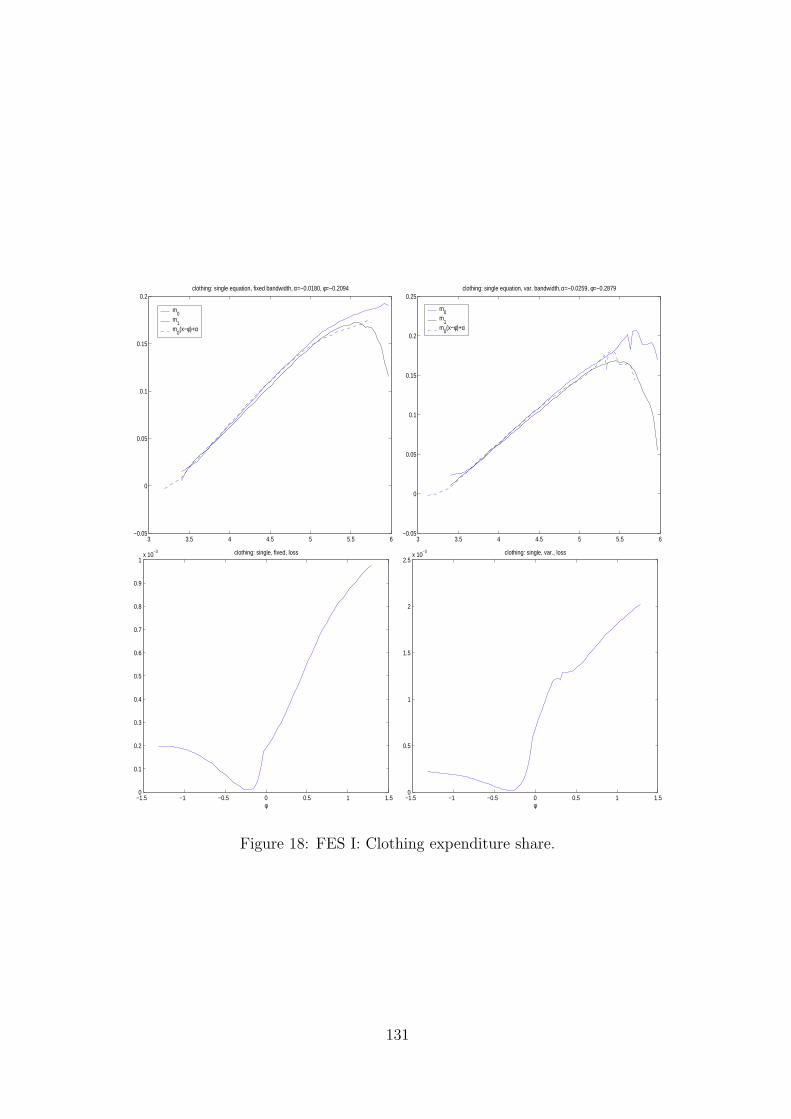
3 3.5 4 4.5 5 5.5 6−0.05
0
0.05
0.1
0.15
0.2clothing: single equation, fixed bandwidth, α=−0.0180, φ=−0.2094
m0
m1
m0(x−φ)+α
3 3.5 4 4.5 5 5.5 6−0.05
0
0.05
0.1
0.15
0.2
0.25clothing: single equation, var. bandwidth, α=−0.0259, φ=−0.2879
m0
m1
m0(x−φ)+α
−1.5 −1 −0.5 0 0.5 1 1.50
0.1
0.2
0.3
0.4
0.5
0.6
0.7
0.8
0.9
1x 10
−3 clothing: single, fixed, loss
φ−1.5 −1 −0.5 0 0.5 1 1.50
0.5
1
1.5
2
2.5x 10
−3 clothing: single, var., loss
φ
Figure 18: FES I: Clothing expenditure share.
131
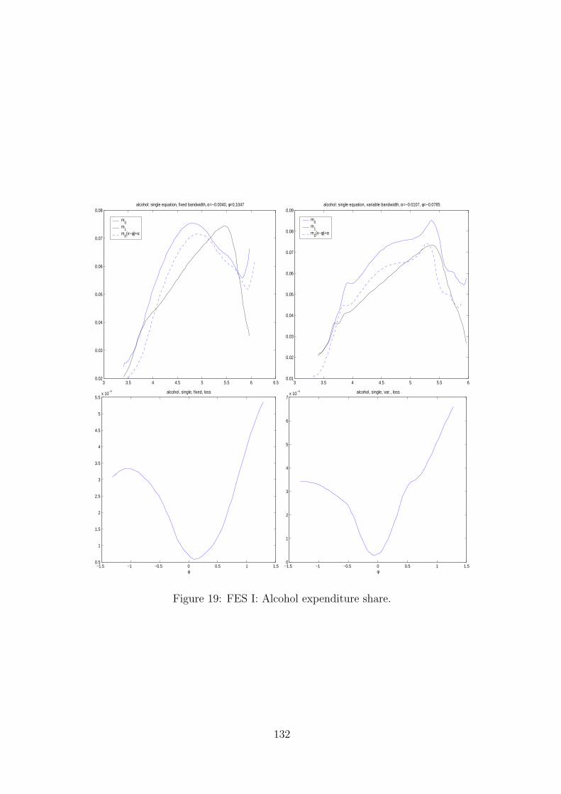
3 3.5 4 4.5 5 5.5 6 6.50.02
0.03
0.04
0.05
0.06
0.07
0.08alcohol: single equation, fixed bandwidth, α=−0.0040, φ=0.1047
m0
m1
m0(x−φ)+α
3 3.5 4 4.5 5 5.5 60.01
0.02
0.03
0.04
0.05
0.06
0.07
0.08
0.09alcohol: single equation, variable bandwidth, α=−0.0107, φ=−0.0785
m0
m1
m0(x−φ)+α
−1.5 −1 −0.5 0 0.5 1 1.50.5
1
1.5
2
2.5
3
3.5
4
4.5
5
5.5x 10
−4 alcohol, single, fixed, loss
φ−1.5 −1 −0.5 0 0.5 1 1.50
1
2
3
4
5
6
7x 10
−4 alcohol, single, var., loss
φ
Figure 19: FES I: Alcohol expenditure share.
132

3 3.5 4 4.5 5 5.5 6 6.50.05
0.1
0.15
0.2
0.25
0.3
0.35
0.4transport: single equation, fixed bandwidth, α=−0.0093, φ=0.0523
m0
m1
m0(x−φ)+α
3 3.5 4 4.5 5 5.5 6 6.50.05
0.1
0.15
0.2
0.25
0.3
0.35
0.4transport: single equation, var. bandwidth, α=−0.0066, φ=0.0785
m0
m1
m0(x−φ)+α
−1.5 −1 −0.5 0 0.5 1 1.50
0.2
0.4
0.6
0.8
1
1.2
1.4x 10
−3 transport, single, fixed, loss
φ−1.5 −1 −0.5 0 0.5 1 1.50
0.2
0.4
0.6
0.8
1
1.2
1.4x 10
−3 transport, single, var., loss
φ
Figure 20: FES I: Transport expenditure share.
133
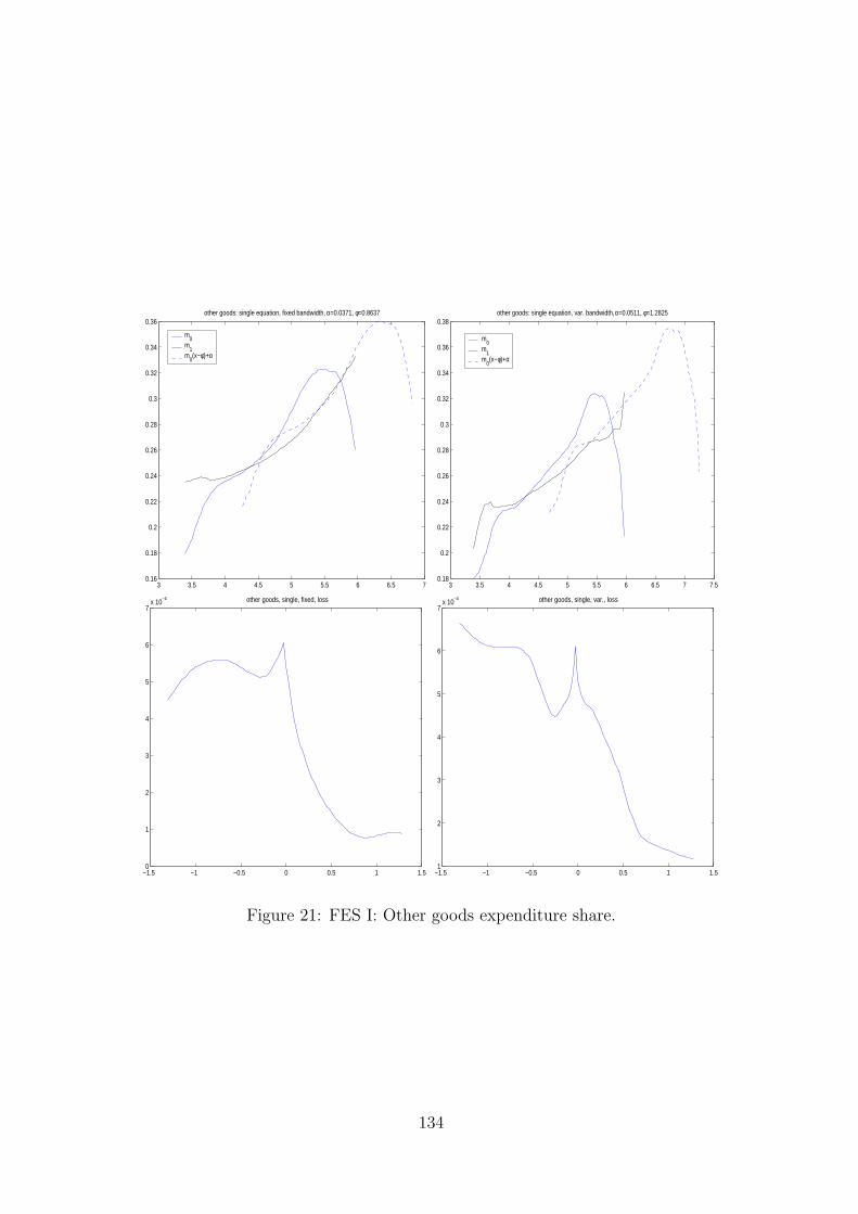
3 3.5 4 4.5 5 5.5 6 6.5 70.16
0.18
0.2
0.22
0.24
0.26
0.28
0.3
0.32
0.34
0.36other goods: single equation, fixed bandwidth, α=0.0371, φ=0.8637
m0
m1
m0(x−φ)+α
3 3.5 4 4.5 5 5.5 6 6.5 7 7.50.18
0.2
0.22
0.24
0.26
0.28
0.3
0.32
0.34
0.36
0.38other goods: single equation, var. bandwidth, α=0.0511, φ=1.2825
m0
m1
m0(x−φ)+α
−1.5 −1 −0.5 0 0.5 1 1.50
1
2
3
4
5
6
7x 10
−4 other goods, single, fixed, loss
−1.5 −1 −0.5 0 0.5 1 1.51
2
3
4
5
6
7x 10
−4 other goods, single, var., loss
Figure 21: FES I: Other goods expenditure share.
134
References
[1] Amemiya, T. (1985). Advanced Econometrics. Oxford: Basil Blackwell.
[2] Blundell, R., Browning, M. and Crawford, I. (1997). Nonparametric Engel Curves and
Revealed Preferences. IFS Working Paper W97/14.
[3] Blundell, R., Chen, X. and Kristensen, D. (2001). Semiparametric Shape Invariant Engel
Curves with Endogeneous Expenditure. Mimeo University College London.
[4] Blundell, R., Duncan, A. and Penkadur (1998). Semiparametric Estimation and Con-
sumer Demand. Journal of Applied Econometrics, Vol.13, No.5,pp. 1-30
[5] Fan,J. and Gijbels, I. (1995). Local Polynomial Modelling and Its Applications. London:
Chapman and Hall.
[6] Hardle, W. and Marron, J.S. (1990). Semiparametric Comparison of Regression Func-
tions. Annals of Statistics, 18, 63-89.
[7] Nadaraya, E. (1989). Nonparametric Estimation of Probability Densities and Regression
Curves. Mathematics and Its Applications. Soviet Series, translated by S.Kotz Dordrecht:
Kluwer Academic Publishers
[8] Pinkse, C. and Robinson, P.M. (1995). Pooling Nonparametric Estimates of Regression
Functions with a Similar Shape. Advances in Econometrics and Quantitative Economics,
eds. G.Maddala, P.Phillips and T.N.Srinvinsan, pp. 172-195.
[9] Wilke, R. (2000). Semiparametric Estimation of Consumer Demand. Discussion Papers
in Economics No. 2000-07, University of Dortmund.
135

“Ich versichere, daß die vorstehende Dissertationsschrift von mir selbstandig ohne
fremde Hilfe und ohne Benutzung anderer als der angegebenen Hilfsmittel angefer-
tigt wurde, und daß ich alle Stellen, die wortlich oder sinngemaß aus veroffentlichten
oder unveroffentlichten Schriften entnommen sind, als solche gekennzeichnet habe.“
136
Recommended