Environmental Magnetic Susceptibility Using the Bartington MS2 System John Dearing This guide has been written to help users of the MS2 Magnetic Susceptibility System gain the most from their equipment. Whilst all reasonable efforts have been taken to ensure that facts are correct and advice given is sound, the user must accept full responsibility for the operation of their equipment and the interpretation of data. The author cannot be held responsible for any damage or loss of equipment, or erroneous interpretation of data arising from the instructions or advice provided in this booklet. John A. Dearing First published 1994 Second edition 1999 All rights reserved. No part of this publication may be reproduced, in any form or by any means, without the permission of the Publisher. ISBN 0 9523409 0 9 British Library Cataloguing in Publication Data. A catalogue record for this book is available from the British Library John A. Dearing has exercised his right under the Copyright, Design and Patents Act, 1988 to be identified as the author of his work and has kindly given permission to Bartington Instruments Ltd to reproduce the original publication with some additional product data. All extracts from this document by any third party must reference the original publication. The original publication remains available through the publisher.

2

Contents Acknowledgements Part 1 Measurement Page • Magnetism and Environmental Materials 4 • Getting started with the MS2B Sensor 11 • Working in the laboratory - sensors MS2B, MS2C, MS2E, MS2G, MS2 κ/T 20 • Surface measurements in the field - sensors MS2D, MS2F and MS2K 27 • Sub-surface measurements in the field – sensor MS2H 30 • Calibration, accuracy and precision 32 • Software for the MS2 35 Part 2 Interpretation • Room temperature susceptibility 36

• Frequency-dependent susceptibility 46 • Low and high temperature susceptibility 48 • Weak samples 52 • References 54

3

Acknowledgements I am indebted to a large number of individuals who, over the years, have discussed with me different aspects of this work. But particularly, I would like to thank the following people. Frank Oldfield and Roy Thompson initiated my interests in the subject and have continued to develop magnetic techniques and extend their application to environmental problems. Geoff and Tessa Bartington read and commented on a number of draft versions, and provided test data and continual encouragement; Tony Clark wrote the section on Archaeological Applications and used his wide experience of geomagnetism to make many improvements to the text; Joan Lees and Rebecca Dann provided me with unpublished experimental data from their PhD research and made extremely useful comments on an earlier version; Karen Hay also made useful comments; Steve Benjamin gave advice on some calculations; and Ruth Gaskell and Kate Phillips prepared the diagrams. I am grateful to Prof. E. de Jong, Barbara Maher and Shaozhong Shi for allowing me permission to use their unpublished results. Some data have been taken from undergraduate student projects in Geography at Coventry University, and I would like to acknowledge the useful works of Paul Bird, Nigel Greenwood, Adrian Lovejoy, Angela Nightingdale, Meg Staveley, Richard Winrow and Andrew Woolnough. Finally, many thanks go to Alix Dearing for proofreading and making corrections. The second edition has benefited from discussions and collaboration with several individuals, especially Cyril Chapman at Bartington Instruments and colleagues in Liverpool; Jan Bloemendal, Bob Jude, John Shaw, Shanju Xie, Yuquan Hu, Amy Clarke and Jack Hannam. Many thanks to Sandra Mather for producing the figure and final copy. On a sad note, Tony Clark died shortly before the completion of the second edition. He was a pioneer of geophysical techniques in archaeological prospecting and a contributor of a section in the first edition. He will be remembered for his dedication and inventiveness and we will all miss his friendliness and generosity. All reasonable attempts have been made to acknowledge original sources of data and to obtain permission to reproduce copyright material. I am grateful to the following publishers and authors for permission to reproduce the following copyright material: John Wiley and Sons Ltd for Figure 3.9 (Dearing, 1992, Earth Surface Processes and Landforms) and Figure 3.11 (Leeks et al, 1988, Earth Surface Processes and Landforms); Geological Society for Figure 3.7 (Kafafay and Tarling, 1985, Journal of the Geological Society of London); Elsevier Science B.V. Amsterdam for Figure 3.15 (Robinson, 1986, Physics of the Earth and Planetary Interiors); American Society of Limnology and Oceanography,In~ for Figure 3.12 (Thompson et al, 1975, Limnology and Oceanography); Scandinavian University Press for Figure 3.8 (Björck et al 1982, Boreas); Edward Arnold Ltd for Figure 3.17 (Williams, 1991, The Holocene); Allen and Unwin Ltd for Figure 3.13 (Richards et al, 1985, Geomorphology and Soils); Chapman and Hall Ltd for Figure 3.6 (Thompson and Oldfield, 1986, Environmental Magnetism); Geological Society of America for Figure 3.14 (Kukla et al, 1988, Geology). Users of the guide are invited to send their comments to the author via Bartington Instruments Ltd. The author will endeavour to respond to all comments received.

4

Part 1 Measurement Magnetism and Environmental Materials Introduction Everything around us is magnetic. As we may describe objects and materials by their size, colour or chemical composition, so we may also describe them by their magnetic properties. This may come as a surprise to anyone without a physics background because in everyday life we usually come across magnetism in rather limited ways, in terms of magnets and metals, or recording tape. We do not think about the magnetic behaviour of rocks or soil, or the dust in the air that we breathe - and most of us would certainly not consider the magnetic properties of river water or leaves on a tree. But all matter is affected by a magnetic field. The effect may be extremely weak or even negative, but it exists and can be measured easily. During the 1970s and 80s, scientists realised that magnetic properties were useful for describing and classifying all types of environmental materials. The Bartington Instruments MS2 Magnetic Susceptibility System became popular for use in the laboratory and field in universities around the world. This book summarises the use of the MS2 System in environmental research and describes how to interpret the data. This first section begins by answering some of the most commonly posed questions about magnetic susceptibility. What can Magnetic Susceptibility do for my studies? First, by considering what magnetic susceptibility can reveal about a material. Magnetic susceptibility measures the ‘magnetisability’ of a material. In the natural environment, the magnetisability tells us about the minerals that are found in soils, rocks, dusts and sediments, particularly Fe-bearing minerals. So the measurements provide information similar to that produced by other mineralogical techniques like X-ray diffraction or heavy mineral analysis. In summary the measurements may enable us to: Identify the Fe-bearing minerals that are present in a sample

Calculate their concentration or total volume with high resolution Classify different types of materials Identify the processes of their formation or transport Create ‘environmental fingerprints’ for matching materials`

There is hardly any area of environmental research where magnetic susceptibility has not been used: a magnetic mineralogical approach is applicable to virtually all kinds of environmental research. The measurements have also been found to be diagnostic of specific processes, like burning or soil waterlogging. These types of diagnostic application are becoming increasingly important to particular areas of study, such as archaeology and soil science.

5

Second, the measurement of magnetic susceptibility is extremely simple and convenient. It is unusual to argue for the use of an analytical technique because it is convenient, but it is a fact that this has been an important reason why researchers have used magnetic susceptibility measurements. The advantages of convenience can be summarised as follows:

Measurements can be made on all materials

Measurements are safe, fast and non-destructive Measurements can be made in the laboratory or field with minimal training

Measurements complement many other types of environmental analyses Large numbers of samples may be measured economically and without limiting subsequent analyses. The measurements are therefore ideal in reconnaissance studies where a large sample set is needed in order to find ‘average’ or ‘typical’ samples for other expensive or time-consuming analyses. Measurements made in situ in the field speed up the process of linking data to field observations, a point that is very important to people working in remote or foreign areas far from laboratory facilities. Therefore, magnetic susceptibility measurements offer a cost-effective option when choosing which analytical techniques to use. Increasingly, magnetic susceptibility is used as one of a number of environmental analytical techniques. For example, it is used in conjunction with analyses of chemistry, radioisotopes, microfossils and remanence magnetic properties. What is Magnetic Susceptibility? The answer to this question can be as simple or difficult as you like! Let us start simply. Magnetic susceptibility, as we have seen, is basically a measure of how ‘magnetisable’ a material is. Take rocks for example. They are made of different minerals or crystals that vary in the strength of their attraction to a small magnet. If the rock was crushed to release the individual crystals we could see this variable effect. Some minerals, such as the iron oxide magnetite, are highly magnetic and jump to the magnet as it is passed across them. Other crystals are attracted to a magnet, but weakly. They stick to the magnet only when it is brought into contact with them. Others like the quartz grains in sand do not show any visible attraction to the magnet. Magnetic susceptibility is basically measuring the total attraction of the first two groups of minerals to a magnet; in other words the rock’s magnetisability. Rocks with relatively high concentrations of magnetite, like basalt, have much higher magnetic susceptibility values than rocks, such as limestone which usually have no magnetite crystals at all. It is not always easy to crush rock and to try this test for oneself. But it is quite easy to demonstrate the presence of highly magnetic minerals in soil. Take a few grams of surface soil and suspend it in a full glass or beaker of water. Rest, or stick with adhesive tape, a small magnet halfway up the side of the beaker and gently swirl the soil and water with a spoon. After a few minutes the highly magnetic minerals should cluster as a small black mass beside the magnet’s poles. If you were to measure the magnetic susceptibility of the soil, the value you obtained would be roughly proportional to the mass of those minerals.

6

Magnetic behaviour To understand exactly why minerals and materials show different responses to a magnet and how magnetic susceptibility is measured we have to enquire into the physics of magnetism. Magnetism is controlled by the inherent forces or energies created by electrons which make up atoms. Electrons spin around their axis, and also around the atom’s nucleus in their own orbits. Spins within spins, analogous to the orbit of the Earth round the Sun whilst spinning on its axis. The way in which different electrons’ motions are aligned determines the total magnetic energy or moment of the atom. Different atoms have different numbers of electrons and types of motion. Atoms make up molecules and molecules make up materials, so that the overall type of magnetic behaviour of a rock mineral is defined by the configuration and interactions of all the electron motions in all its atoms. There are five different kinds of magnetic behaviour. The first of these covers the most highly magnetic substances, like pure iron, and is termed ferromagnetism. Here the magnetic moments are highly ordered and aligned in the same direction. These substances have a very high magnetic susceptibility, but will not normally be found in the environment. The Bartington MS2D search loop can locate buried rusty cans and other items of metallic rubbish easily, and so it is as well to check that high values are from natural minerals. The most important category of magnetic behaviour in natural materials is ferrimagnetism. The magnetic moments are strongly aligned, but exist as two sets of opposing but unequal forces controlled by the crystal lattice structure of certain minerals. This category includes magnetite and a few other Fe-bearing minerals with high magnetic susceptibility values. Magnetite is a common mineral found in all igneous rocks, most sedimentary rocks and nearly all soils. Where these minerals are present they often dominate the magnetic susceptibility measurement. Lower magnetic susceptibility values are obtained for canted antiferromagnetic iron minerals, such as haematite. Here the crystal structures also give rise to well-aligned but opposing magnetic moments, but the forces virtually cancel each other out. There are only a few minerals in this category and haematite is probably the most common, occurring in many rocks and soils, and responsible for much of the natural red colouration in the environment. All metals and minerals in these three magnetic groups are able to remain magnetised in the absence of a magnetic field and may be identified using remanence measurements. Similar or weaker magnetic susceptibility values are obtained for a group of minerals with the property of paramagnetism. The magnetic moments arising mainly from the presence of Mn and Fe ions are aligned only in the presence of a magnetic field. There are a large number of these minerals that normally contain iron, and are very common in rocks and soils. Examples are biotite and pyrite. Finally, there is a category of magnetism referred to as diamagnetism. Here the magnetic field interacts with the orbital motion of electrons to produce weak and negative values of magnetic susceptibility. Materials which fall into this group include many minerals which do not contain iron, like quartz and calcium carbonate. Other non-mineral diamagnetic substances are organic matter and water. Therefore, the magnetic susceptibility of an environmental material is the sum of all the magnetic susceptibilities of the ferrimagnetic, canted antiferromagnetic and paramagnetic minerals and diamagnetic components. Normally, the diamagnetic component is negative and very weak relative to the sum of the other three and can be ignored. Exceptions to this are where the sample is almost all water, quartz or organic matter.

7

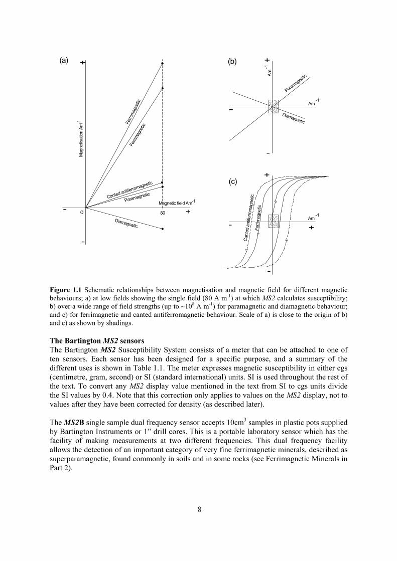
How can we visualise the concepts of magnetic fields, magnetisation - and a measurement of magnetic susceptibility? One way is to think of a magnetic field as lines of force shown by iron filings lying between the N and S poles of a magnet. When an unmagnetised sample is placed into the magnetic field the sample will become magnetised with its own invisible lines of force and affect the total number of lines that were originally there. Different substances and environmental samples will affect the force lines in different ways. Diamagnetic water will become weakly magnetised in the opposite direction to the applied field and so reduce the total number of lines, while a lump of basalt rock with many ferrimagnetic minerals will become highly magnetised in the same direction as the lines of magnetic field and will greatly increase the total number of force lines per unit area. The total magnetic force in the material while it is in a magnetic field is called the magnetisation. For each substance there is a relationship between the magnetic field and the amount of magnetisation created. In weak magnetic fields the relationship is effectively linear and is defined by the gradient of the line or, in the case of the MS2B sensor, the ratio of the strength of the magnetisation (A m-1) to a magnetic field of ~80 A m-1. This ratio is the magnetic susceptibility and is shown schematically in Figure 1.1a for the different types of magnetic behaviour and minerals described above. Consequently, each Bartington sensor creates a weak magnetic field from an alternating current (AC) and detects the magnetisation of the material lying in it. The magnetic susceptibility is calculated and its value is shown on a digital display. All Bartington sensors measure magnetic susceptibility relative to air which is used to zero the meter. More advanced magnetic measurements using magnetometers make use of the relationship between magnetisation and magnetic field at progressively higher field strengths in positive and negative directions, and the amount of remanent magnetisation measured after a magnetic field has been reduced to zero. Measuring magnetisation at a range of magnetic fields gives rise to a range of relationships ranging from linear (paramagnetic and diamagnetic - Figure 1.1.b) to the non-linear hysteresis loop (ferrimagnetic and canted antiferromagnetic - Figure 1.1c), each one often diagnostic of the type of magnetic behaviour and sometimes the mineral, but where low field magnetic susceptibility remains its fundamental property.

8

Figure 1.1 Schematic relationships between magnetisation and magnetic field for different magnetic behaviours; a) at low fields showing the single field (80 A m-1) at which MS2 calculates susceptibility; b) over a wide range of field strengths (up to ~108 A m-1) for paramagnetic and diamagnetic behaviour; and c) for ferrimagnetic and canted antiferromagnetic behaviour. Scale of a) is close to the origin of b) and c) as shown by shadings. The Bartington MS2 sensors The Bartington MS2 Susceptibility System consists of a meter that can be attached to one of ten sensors. Each sensor has been designed for a specific purpose, and a summary of the different uses is shown in Table 1.1. The meter expresses magnetic susceptibility in either cgs (centimetre, gram, second) or SI (standard international) units. SI is used throughout the rest of the text. To convert any MS2 display value mentioned in the text from SI to cgs units divide the SI values by 0.4. Note that this correction only applies to values on the MS2 display, not to values after they have been corrected for density (as described later). The MS2B single sample dual frequency sensor accepts 10cm3 samples in plastic pots supplied by Bartington Instruments or 1” drill cores. This is a portable laboratory sensor which has the facility of making measurements at two different frequencies. This dual frequency facility allows the detection of an important category of very fine ferrimagnetic minerals, described as superparamagnetic, found commonly in soils and in some rocks (see Ferrimagnetic Minerals in Part 2).

- 0 +80

-

+

Magnetic field Am-1ParamagneticCanted antiferromagnetic

Ferri

magn

eticFe

rrom

agne

tic

Mag

netis

atio

n Am

-1

(a) (b)

(c)

+

-

-Am

-1

Am-1

Paramagn

etic

Diamagnetic

+

+

-

-Am

-1

Ferri

mag

netic

Cant

ed a

ntife

rrom

agne

tic

Diamagnetic

9

The MS2C core-scanning sensor is designed to measure the magnetic susceptibility of material in cores as extracted. The sensor comes in a range of sizes to accommodate different kinds of cores. The MS2C has been successfully used in the laboratory and field locations including fieldwork campsites and deep-sea drilling vessels. Both the MS2D and MS2F sensors comprise a loop/probe attached to a handle with an electronics unit, through which the MS2 meter is attached. The MS2D search loop sensor is a field sensor, 185 mm in diameter, designed to make surface measurements of soils, rocks, stream channels etc. It is simple and quick to use and is employed mainly in mapping and reconnaissance surveys. The MS2E sensor measures the susceptibility of surfaces (usually fresh cores covered with plastic film) at a high spatial resolution (3.8 mm). It has proved very successful in identifying turbidites in Lake Baikal sediments and mineral characteristics of laminated sediments from Greenland. The MS2F probe sensor is also a field sensor, but designed to measure smaller scale variations in the magnetic susceptibility than the search loop. It is used to measure the susceptibility variations in geological exposures, soil pits and in individual stones and clasts. The MS2G sensor is for small single samples measured at low frequency only. The sensor accepts commercially available polythene tubes (typically 33 mm x max. diameter 8 mm) with a nominal calibration volume of 1 cm3. A calibration sample is provided. Early trials on soil and sediment samples suggest that susceptibility measurements may be made on small samples (~0.2 cm3) with little loss of sensitivity compared with the 10 cm3 MS2B dual frequency sensor. The sample holder’s shape and size are also compatible with other rock magnetic measuring equipment, such as the Molspin vibrating sample magnetometer and various pulse magnetisers, allowing for a fuller range of measurements without the need for re-packing. The MS2H sensor is a sub-surface probe for profiling the magnetic susceptibility of strata in 25mm nominal diameter auger holes. Extension tubes allow measurements to depths of 2 or 3 metres. The spatial resolution of the probe is 1.5cm and tube graduations ensure depth control to a resolution of 1cm. Applications include cultural stratigraphy in archaeology, landfill studies and landslide characterisation. The MS2K sensor is designed to provide highly repeatable surface measurements on moderately smooth surfaces. It is used for magnetic stratigraphy, identifying horizons, characterising outcrops and logging plastic film covered split cores. The MS2 κ/T system permits susceptibility measurements to be made on 15 mm (2.5 cm3) samples from -200 °C to +850 °C. It is used to detect magnetic responses to temperature, notably Curie points and low temperature transitions, which enable identification of mineral type (see Low and high temperature susceptibility). The MS2W sensor which fits around the sample furnace is water-cooled to give excellent temperature stability during the heating and cooling cycle. The sensor is connected to the MS2 meter and is used in conjunction with the MS2WFP power supply.

10

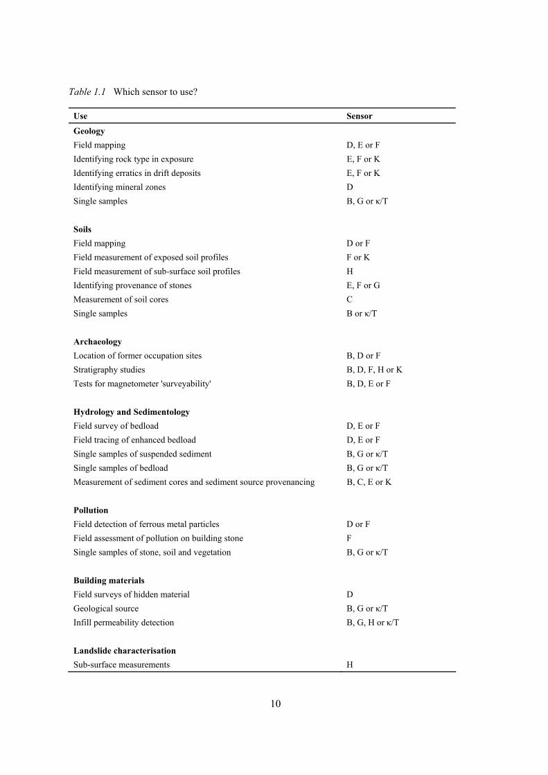
Table 1.1 Which sensor to use?

Use Sensor

Geology Field mapping D, E or F Identifying rock type in exposure E, F or K Identifying erratics in drift deposits E, F or K Identifying mineral zones D Single samples B, G or κ/T Soils Field mapping D or F Field measurement of exposed soil profiles F or K Field measurement of sub-surface soil profiles H Identifying provenance of stones E, F or G Measurement of soil cores C Single samples B or κ/T Archaeology Location of former occupation sites B, D or F Stratigraphy studies B, D, F, H or K Tests for magnetometer 'surveyability' B, D, E or F Hydrology and Sedimentology Field survey of bedload D, E or F Field tracing of enhanced bedload D, E or F Single samples of suspended sediment B, G or κ/T Single samples of bedload B, G or κ/T Measurement of sediment cores and sediment source provenancing B, C, E or K Pollution Field detection of ferrous metal particles D or F Field assessment of pollution on building stone F Single samples of stone, soil and vegetation B, G or κ/T Building materials Field surveys of hidden material D Geological source B, G or κ/T Infill permeability detection B, G, H or κ/T Landslide characterisation Sub-surface measurements H

11

Getting started with the MS2B Sensor The first ten minutes in button mode A good way to start is to measure the 10cm3 calibration sample (containing a small ferrite bead) provided by the manufacturer. This is used to check the long term calibration of the MS2 meter. It is a ferrimagnetic material with a moderately high magnetic susceptibility. The value of susceptibility is recorded on the plastic pot in cgs and SI units (SI = cgs value * 0.4; in dimensionless SI units . 10-5) . Refer to Figure 1.2 and follow these steps. 1. Connect the MS2B sensor to the meter as explained in the Operation Manual, making sure

that the connections are not overtightened. 2. Turn the right-hand range multiplier switch to BATT. Only proceed to the next steps if a

green light shows, otherwise recharge batteries in MS2 meter as described in the Operation Manual.

3. Turn the on/off switch to SI. Choose the 1.0 range on the range multiplier switch. 4. Turn the knob on the MS2B sensor to LF. Now there should be some numbers on the

display. 5. Make sure that the toggle switch below the buttons is in its central position. Leave the

system to ‘warm up’ for ten minutes.

Now you are ready to make measurements in button mode using the push buttons marked Z for zero and M for measurement.

6. Push the zero button Z watch the display clear, and wait 1-2 seconds for a bleep. There

should be a series of zeroes, like this (0000). 7. Raise the handle of the insertion mechanism on the sensor and place the calibration sample

in the sample holder, with its lid uppermost. 8. Ensure that the holder sits into the cut-outs on the insertion mechanism. Lower the sample

back into the sensor. 9. Push the measuring button M. You should see a double-dot colon appear between the

zeroes (00:00) which shows that the meter is busy or measuring. After the bleep, note the new value on the display. It should be very close to the calibration value (converted to SI units). Like this, (0150) i.e. 150 SI units.

10. Raise the insertion mechanism and remove the sample. 11. To repeat the measurement simply replace the sample and push M. There is no need to

push Z between repeat measurements or between different samples.

12

Now that you have obtained a satisfactory display value for the calibration sample we can pause to consider what you have measured. The instrument has done three things. It has created a magnetic field, it has detected the magnetisation in the sample, and calculated the ratio or magnetic susceptibility between the two. The value on the display is called volume susceptibility or κ (Greek k or kappa) and represents the ratio of the magnetisation to field (80 A m-1) in the SI scheme. It happens that magnetic fields and magnetisation per unit volume have the same units (A m-1) in the SI scheme (see Figure 1.1). Therefore κ has no units and is referred to as dimensionless. Values of κ on the MS2 meter do have a scale, though, which in the case of SI is 10-5 So the volume susceptibility value for the calibration sample is 150 x 10-5 (or whatever the value was for your sample). Repeat the steps a few times and see what the variations are. They should not be very large, perhaps varying by 1 or 2 units which would give an error on the mean value of less than 2%. Any small variations in the κ value for the calibration sample are due to the initial zero measurement or the air measurements not being exactly zero. This is usually due to a combination of a less than ideal working environment and a small amount of drift in the instruments (see Working in the laboratory). In samples which have moderately high κ values, >100, the variations may be insignificant and acceptable. In weaker samples or where the highest accuracy is required, you will have to correct for the non-zero air readings (see Measuring weak samples). Push buttons Digital Display ON/OFF and Battery Indicator SI/cgs units and range multiplier

Measure Toggle Switch for Zero Decimal point Power continuous mode when in 0.1 range

Figure 1.2 The MS2 meter display panel What you have done so far is to make a number of measurements of κ on the calibration sample in SI units at the rapid 1.0 range. There are other measuring options available which may be more suitable for other samples. The next section covers four other types of measurements, on very strong samples, on weak samples, calculating mass specific susceptibility values and using the dual frequency option. If you want to follow the instructions closely you will need to obtain other samples. Table 1.2 describes some common samples which are used in the text and their preparation - but you can substitute other materials with similar susceptibility values or move on directly to your own environmental samples.

13

Table 1.2 Samples with different magnetic behaviour Material Magnetic Behaviour Water Diamagnetic Calibration Sample Ferrimagnetic ‘Ferro’ Cassette Tape Ferrimagnetic Steel Wool Ferromagnetic Preparation: Weigh four 10 cm3 pots with their lids on a laboratory balance in grams (g) to 3 decimal places and fill the pots with the samples. With water and cassette tape you should completely fill the pots, but with the steel wool you should just use a small piece teased out to fill most of the pot. Replace the lids and re-weigh the pots with their samples. Calculate the sample masses by subtraction. Notes on materials: • Tap water will do. • The calibration sample is provided by the manufacturer, and is normally a sample containing a

small ferrite bead. • Use normal type 1 cassette tape made of iron oxide, often known as ‘ferro’ tape, which is usually

made with maghemite minerals, γFe2O3. Do not use ‘metal’ tapes with chromium or other metals. Normal ‘ferro’ tapes are usually the cheapest!

• Use any ordinary steel wool or ‘Brillo’ pad type scourers. Make sure that the steel wool is pulled

apart before putting into the sample pots. Rusted steel wool will have a much reduced κ value, so only use fresh material.

Table 1.3 Typical volume susceptibility values of samples Material Mass

(g) Volume Susceptibility (K)

(dimensionless)

Water 10.0 -0.9 Calibration sample 12.0 150 ‘Ferro’ cassette tape 1.0 1000 Steel wool 2.5 4000 These values obtained by the author should only be taken as a guide to the magnitude of κ values.

14

Continuous measurement mode and strong samples You are now ready to start measuring other samples. Start with a sample of ‘ferro’ cassette tape. This type of cassette tape is made from a manufactured iron oxide, called maghemite, stuck to a plastic base. The same mineral occurs naturally in soils and rocks and is ferrimagnetic. Measure the sample as before using the button mode. You should get a high value of several hundreds or even over a thousand depending upon the mass of the sample. Table 1.3 shows κ values for this and the other samples obtained by the author. An alternative way is to make measurements in continuous mode using the toggle switch below the M and Z buttons (refer to Figure 1.2). The toggle switch has three positions; central for when the M and Z buttons are used, right for zero (in the direction of Z) and left for measurement (in the direction of M). With the meter set in SI and 1.0 ranges and the sensor in LF mode follow these steps: 1. With the insertion mechanism empty, push the toggle switch towards the right, wait for a

bleep and push back across the central position towards the left to make a measurement of air.

2. Let the meter measure air continuously. Watch to see if the air values change at each bleep.

If the values are not very close to zero, move the toggle switch back to zero, wait for the display to clear and repeat the measurements of air.

3. Without touching the toggle switch or buttons, lift the insertion mechanism, seat the pot of

cassette tape and lower it into the sensor.

4. Watch the meter display the continuous measurements of the sample. After two or three bleeps the values should stabilise. Note the value and remove the sample.

The value which you obtain should be identical to the value obtained in button mode. This measurement method is not often used in the laboratory and is most used in the field with the search loop and probe sensors. There is one exception - very strong samples. With very strong samples there is a risk that the meter will overload and not display the correct value. This is because the meter can display values only up to (9999). Higher values are truncated so that the first digit in tens of thousands is lost. Ferromagnetic materials, such as steel wool, have very high susceptibilities and you can see from Table 1.3 that a 2.5 g sample will have a display value for κ in the thousands. Measure a sample of steel wool in button mode and note its value. Now repeat the measurement in continuous mode but lower the pot of steel wool slowly into the sensor and watch the display to see the values increase at each bleep. By watching the values rise you can see if your sample is going over the (9999) limit. If it is, remove the pot and reduce the amount of steel wool to get a value of less than (9999). If your sample is not that strong then you should find the meter reading settling on the value you obtained in button mode. Ferromagnetic substances and values in thousands on the display are very rare in natural environmental samples, and normally indicate the presence of ferrous metal in the sample.

15

Measuring weak samples on the 0.1 scale So far you have measured samples with relatively high κ values. Let us turn our attention to weaker substances which include the majority of soils, sediments and rocks. If a sample has a fairly small κ value of 10 to 30, repeated measurements will probably show values varying by about 1 SI unit. This variability means that a κ value of 20 will have an error of 5 to 10%. This error is unacceptably high for most purposes and shows that, as a general rule, materials giving κ values of about 50 or less should be considered as weak samples and should be measured on the higher sensitivity range. Small increments of instrumental drift between readings are now more important and have to be corrected for. Measure the calibration sample again, but follow this sequence: 1. With the sensor empty turn the range multiplier to 0.1 and check that the toggle switch is

central. 2. In button mode push Z to zero. The meter now takes a longer time to clear the display or to

make a measurement, as you can hear in the time interval of about 12-13 seconds between bleeps.

3. Push M to make a measurement of air. This is what we refer to as the first air reading and

should be close to zero. On the 0.1 range there is a decimal point, so the smallest number on the display is 0.1. Thus nought point one is (000.1) and minus one point two is (-01.2).

4. Lower the sample into the sensor. Push M to measure the sample. After the bleep remove

the sample and note the sample value. 5. With the sensor empty, make a second air reading using the M button.

6. As before, you do not need to zero the meter before measuring the next sample. You now have three readings; a first air reading, a sample reading and a second air reading. Ideally, the first and second air readings should be zero. If they are different, your sensor is drifting slightly during the time taken to make the three readings. You should correct the sample reading by subtracting the mean of the two air measurements, like this:

κ (corrected) = sample κ - {(first air κ + second air κ)/2} Sometimes the average of the air values is negative, so don’t forget that a ‘minus minus’ is a plus! If you found it difficult to obtain a first air value of zero, it is most likely that either you have not let the meter and sensor warm up properly or that there is some metallic material close to the sensor (see Working in the laboratory). It is also important that the time between the measuring cycles is kept short and as constant as possible. This requires practice on the part of the operator to order to obtain a standard handling and measurement procedure.

16

Finally in this sample run, make a measurement in button mode for a 10 g sample of water. Table 1.3 shows that water is diamagnetic, and that we expect to get a very weak and negative volume susceptibility of -0.9 x 10-5. Other diamagnetic materials in the natural environment include chalk, limestone, quartz and vegetation. These types of samples require the most careful of measurement procedures if an accurate and precise value is to be obtained. See how close you can get to the expected value. Remember to check carefully the calculations which include negative numbers. Repeat the measurement nine times more and calculate the mean of the ten corrected κ values. The range of corrected numbers you have more or less defines the precision of the measurements you can make with your meter and sensor in its present operating environment (see Calibration, accuracy and precision). If you feel that the drift between air measurements is too large, you may need to improve the operating environment. It is often necessary to measure very weak samples a number of times to get a precise mean value. When samples are weak, the diamagnetic properties of the sample pot and the insertion mechanism may contribute significantly to the susceptibility, with the effect of reducing the true value. It is recommended that a selection of pots are measured empty in order to obtain a mean diamagnetic κ value at the 0.1 range. It is typically -0.4 x 10-5 SI for the standard 10 cm3 pot. This value can be added to all sample κ values. Where high precision is required the correction should be specific to individual pots. Make a correction for the water sample and see the effect it has on the κ value. Mass Specific Susceptibility By now you should have measured a number of samples and obtained a variety of volume susceptibility values (κ). You will have probably realised that your samples are of different masses and shapes, and that these may account for some of the differences in κ values. We know that large samples will show higher κ values than small samples of the same material. Environmental studies often measure materials which have widely different bulk densities. This may be for several reasons. For instance, the water content of soil can be very variable. Some materials simply lie at the extreme ends of the range of bulk densities, like samples of dried peat and iron ore. Other samples have different densities because of the way they have been prepared or packed into pots. Therefore single sample susceptibility is not normally expressed on a volumetric basis, but on a basis of dry mass. Some studies have used single homogeneous sample κ values, notably studies of deep sea sediments, but only where density is fairly constant or where κ data are used to form ratios which are independent of density. In order to obtain mass specific susceptibility the κ value is divided by the bulk density of the sample. The bulk density of a sample is calculated by dividing mass by volume. This is easier to calculate than it seems because all the MS2B samples are usually measured in pots of 10 cm3. So provided that the pots are full, only the mass values vary (see MS2B sample size). Take the example of water. You should have a κ value of about -0.9 x 10-5 for 10 cm3. The mass will be about 10 g, giving a bulk density of about 1 g cm-3. It looks as if it is necessary to divide the κ value by 1. But be careful! The SI units for bulk density are in terms of kg m-3, not g cm-3. And in these units, water has a bulk density of 1000 kg m-3. Therefore we should divide the κ value by 1000, not 1. Like this:

(-0.9 x 10-5)/1000 = -0.9 x 10-8

17

What about the values? Are they still dimensionless? The answer is no. The κ value has now been divided by kg m-3, which means that the new value has units which are 1/(kg m-3) or the reciprocal of kg m-3, which is m3 kg-1. So the value of -0.9 x 10-8 has units of m3 kg-1. This new adjusted value is known as mass specific susceptibility and is given the symbol χ (Greek X or chi). In formula terms:

χlf = κ/ρ

where χlf is the low frequency (lf) mass specific susceptibility (m3 kg-1), κ is volume susceptibility and ρ is the sample bulk density (kg m-3). In practice, three points are worth mentioning. First, the SI convention is to express units on scales varying by factors of a thousand (e.g. 10-3, 10-6 or 10-9) so that the units for mass specific susceptibility of 10-6 m3 kg-1 are most commonly used, though some groups of workers prefer units of 10-8. Second, the use of the symbol μ (mu) as an alternative to 10-6 is wrong in this case because the symbol should refer to the next unit (i.e. m) not the scale. Third, if all the volumes are about 10 cm3, you can get the right answer in 10-6 m3 kg-1 by simply dividing κ by sample mass and then dividing by 10 (see MS2B sample size and volume). Try this calculation for the ‘ferro’ cassette tape and water and compare your answers with those in Table 1.4. (Note that the χlf value given for the steel wool is not strictly accurate because the true volume of steel in the pot was much less than 10 cm3). Care should be taken where samples have volumes which are not 10 cm-3 (see MS2B sample size). Table 1.4 Mass specific susceptibility of samples Material Mass (g) Volume susceptibility (κ)

(dimensionless) Mass specific

susceptibility (κ) (10-6 m3 kg-1)

Water 10.0 -0.9 -0.009 ‘Ferro’ tape 1.0 1000 100.0 Steel wool 2.5 4000 160.0 The χlf values assume a 10 cm3 sample volume. Frequency Dependent Susceptibility Measurements of frequency dependent susceptibility involve making two κ readings in magnetic fields created at two different frequencies (0.46 and 4.6 kHz). The measurements are used to detect the presence of ultrafine (<0.03 μm) superparamagnetic ferrimagnetic minerals occurring as crystals produced largely by biochemical processes in soil. Samples where ultrafine minerals are present will show slightly lower values when measured at high frequency; samples without the minerals will show identical κ values at the two frequencies. The switch on the front of the MS2B sensor allows the choice of low frequency (LF) or high frequency (HF) ranges.

18

Calibration of the LF and HF ranges is carried out at the factory and should not be needed again. You can check this by measuring the calibration sample at both frequencies in button mode at the 1.0 range. Measure the sample once on LF, as before. Remove the sample, switch to HF, re-zero and re-measure. The ferrimagnetic calibration sample contains a negligible amount of ultrafine minerals and therefore should show no significant difference in κ values at LF and HF (κlf and κhf). The difference in the corrected values should be less than 1%. If the difference is greater there may be a need to cross-calibrate the electronics of the two circuits, as described in the manufacturer’s instructions. None of the samples in Table 1.3 will show significant differences between κlf and κhf. The best type of material for showing significant frequency dependence is fertile, minerogenic topsoil from a well-drained site. Differences between values at κlf and κhf should range between 5 and 15% of the κlf value. In practice, all measurements should be made on the 0.1 range unless the display values are in the hundreds. Differences which are important are normally of the order of 1-10% and as much accuracy and precision as possible is required. This means that some samples are too weak for dual frequency measurements. We can estimate just how weak by assuming that the highest precision is ± 0.1 on each reading. Thus the smallest significant difference between the LF and HF readings is ~0.4 units. On a κlf value of 50.0, this difference represents 0.8%, on a κlf value of 25.0 it represents 1.6%, and on a κlf value of 10.0 it represents 4.0%. As a general rule, samples with κlf values <10 cannot provide useful dual frequency data, and even samples with κlf values 10-25 are prone to large errors. If it is essential to obtain dual frequency data on weak samples it will be necessary to use the mean values of ten or more κlf and κhf measurements. It is recommended that all samples are measured on the LF range first. Then select HF, re-zero and re-measure all the samples on the HF range. For maximum resolution, wait a few minutes after switching between LF and HF on the sensor before making measurements. It is a good policy to measure the samples in the two frequencies in the same orientation. This is easily done by keeping the tab or a mark on the sample pot to the front or some other point, and reduces the chance of small directional variations in susceptibility affecting the readings. Frequency dependent susceptibility may be expressed either as a percentage of the original LF value or as a mass specific frequency dependent susceptibility value for the frequencies of the sensor. The importance and need for one or the other is a matter of judgement; the calculations are simple expressions of the same data in relative and absolute forms analagous to the type and concentrations of magnetic minerals respectively (see Part 2). Percentage frequency dependent susceptibility (κfd% or χfd%) is:

(κlf -κhf/κlf) x 100 where κlf is the corrected reading at low frequency and κhf is the corrected reading at high frequency.

19

Alternatively, mass specific dual frequency dependent susceptibility (χfd) is:

χfd = (κlf-κhf)/ρ where χfd is the mass specific frequency dependent susceptibility (m3 kg-1), ρ is the sample bulk density (kg m-3). Similarly to the calculation of χlf , dividing by mass and then by 10 gives values in the units 10-6 m3 kg-1. Most workers prefer to multiply the 10-6 values by 1000 and to express in SI units of 10-9 m3 kg-1. The use of n (nano) as a substitute for 10-9 is wrong in this context. Summary of measurements and ranges Table 1.5 summarises the modes of measurement described in the text and the different multiplier ranges which should be used for different ranges of display values. For example, samples with a κlf value of <100 should be measured for frequency dependent susceptibility on the 0.1 multiplier range. Some workers may choose different threshold values, especially if they possess older equipment which may not be as stable as the modern sensors. Table 1.5 Measurements, display κ values and multiplier ranges (SI) Range Multiplier X 0.1 X 1.0 MS2B LF button mode 0.1-50 >50 MS2B LF continuous mode >1000 MS2B dual frequency 10-100 >100 The x 0.1 range assumes making corrections for drift by taking two air readings

20

Working in the laboratory - sensors MS2B, MS2C, MS2E, MS2G, MS2 κ/T Finding a ‘quiet environment’ With all sensitive equipment there are ways of making sure that you are getting the most accurate measurements. The most sensitive parts of the MS2 system are the sensors, and every effort should be made to use them within a suitable ‘quiet’ environment. The sensors are affected by the presence of magnetic materials, electromagnetic fields and changes in temperature. The following points should be taken into account when installing a laboratory sensor.

Keep stable by retaining the sensor in wooden or plastic frames or by standing the sensor feet in recesses. Keep away from metal objects, screws and nails in the table. Keep away from the MS2 transformer and mains cable. Keep away from electronic devices especially electric motors and other field generating devices. Keep away from vibrations, such as other motors on bench or lift shafts. Keep away from draughts, sunlight and any other source of intermittent heat. Keep the ambient working temperature cool and as constant as possible.

Variable ambient temperatures will affect the stability of the sensor, especially at high room temperatures. Cool room temperatures controlled by air-conditioning or fans are preferred. Temperature also affects the magnetic properties of samples by causing the boundary between superparamagnetic and single domain grains (Curie-Weiss law) to shift to larger grain sizes as temperature increases, thus increasing the proportion of superparamagnetic grains. A 5-10°C difference in room temperature between runs of measurements made using a MS2B sensor at different times or in different laboratories may be sufficient to give non-comparable values of χlf, χfd and χfd % in samples with a large superparamagnetic component. Once you are satisfied with the location of the meter and its sensor, it is recommended that the sensor should be allowed to measure air continuously over a long period in the 0.1 range. This will let you see the nature of the sensor’s drift and may help to identify the presence of irregular magnetic fields or vibrations which affect the sensor’s performance. If possible you should obtain air readings for several hours during a typical working day. The modern MS2 sensors are very stable, and drift should not prove to be a problem except when dealing with extremely weak samples or where the operating environment is highly detrimental to the sensor’s stability. Studies of long sequences of air measurements suggest that the MS2B sensor should be switched on for about 10 minutes before measurements are made. If the drift is irregular or ‘noisy’ try different operating environments and even different times when the intensity of electromagnetic fields from transmitters, electric motors and electric cables is lower. Several users have found night time measurements in rural areas much less noisy than during daytime in the middle of a city.

21

Coins, rings, jewellery, metal buttons etc. can all affect measurements. If measurements are being noted by hand, make sure that the pen is not brought near the sensor. Avoid touching the sensor; the change in heat is enough to alter its stability. MS2B and MS2G sample preparation All sampling should be carried out in ways designed to minimise contamination from ferrous metal. In the field this means avoiding the use of iron spades, trowels and coring devices or at least taking samples from materials not in direct contact with the metal. Plastic or nylon implements are the best alternatives where possible. Children’s spades and plastic spoons are all basic kit for the environmental magnetist! Implements built from stainless steel and aluminium provide a much reduced risk of contamination, but all users should measure scrapings of the metals to gauge the risk. Samples taken from air filters or sieving machines should be compared to samples of ‘non-magnetic’ powders, such as aluminium oxide, after the same treatment. Samples can be measured dry or wet, even if the liquid present is highly conductive like sea water. Freeze drying of samples is convenient and provides a friable dry sample for easy packing into sample pots. Air drying is best carried out at normal room temperature (25°C). If rapid drying is desirable, then oven-drying to 35°C is acceptable - but ensure good air circulation and no hotspots in the oven. Some important mineralogical changes can occur on air drying through oxidation, especially where the sample is reduced and contains iron sulphides. Also thermal alteration may occur in some iron hydroxides at 40-50°C. If in doubt about the effects of temperature or drying then it is best to compare measurements on wet and dry samples, and to dry out the wet samples after measurement. Many of the commercially available plastic sample pots can withstand temperatures up to 40°C and therefore samples can be oven-dried in their sample pots. But refer to the manufacturer’s specifications before placing any plastic sample pot in an oven: there is a significant fire risk. All samples should be allowed to reach the same room temperature before they are measured. The use of the MS2E sensor to measure frozen core samples, for instance, could produce significant effects on sensor stability. If measurements are essential for single frozen samples, the insulated MS2W sensor of the κ/T system should be used. The temperature effects on drift should be evaluated using samples of ice and water. Dried samples can be packed into sample pots in any convenient way as long as the material is not contaminated. The use of plastic spatulas or small spoons is recommended for dried soils and sediments. There are a number of advantages in wrapping the samples in plastic film before placing into sample pots:

Easy transfer to other sample holders without loss of samples. Loose samples can be wrapped tightly and extra packing added if necessary to restrict sample movement between measurements at two frequencies (and in subsequent spinner magnetometers). Small wrapped samples may be measured together in the same sample pot without physically mixing them together. Small volume samples may be supported on a plastic film pad and positioned in the central zone of a sample pot (see below).

22

Custom-built presses with nylon heads have been used for packing samples into pots. Often samples need to be broken down after air or oven drying, and a ceramic pestle and mortar are useful for this. If the dried material is very solid and tough to break, it can be hammered by wrapping in a few layers of plastic first. Rock samples have been cored and cut using fine diamond blades and bits, and contamination seems to be negligible if the samples are well-washed and scrubbed to remove metallic chaff. Ball mills using glass or ceramic beads inside a revolving drum have been successfully used to break down soils. Where steel or metallic implements are used during the sampling or packing procedures it is essential to assess the chance of contamination by testing with diamagnetic silica sand or some other ‘non-magnetic’ material and measuring before and afterwards. Remember that invisible quantities of iron or rust can produce a significant and measurable contamination. Samples of fine material can be measured directly on pre-weighed filter papers, and this is a common approach for measuring suspended fluvial sediments. Blank filter papers must be measured for control because some, especially glass-fibre filters, are magnetically ‘dirty’. The filter paper should be folded in a constant way to ensure that each sample has the same geometry and is distributed as far as possible throughout the whole volume of the sample holder (see MS2C sample size). An alternative approach is to cut disks of filter paper and to stack them in a sample holder. Disks can often be cut using an upturned standard holder as a cutter. This approach has been successfully extended to the study of leaves contaminated with pollution or dust particles. MS2B and MS2G sample size and volume As explained in the Mass specific susceptibility section there will be an error in the calculation of κ and χlf if a 10 cm3 sample pot is not full or if non-standard sample pots are used. But how full is full? Can we forget about small differences in volume? Sample size and volume errors can be calculated by filling a range of pots with different volumes of a well-mixed paramagnetic reagent, like manganous carbonate (MnCO3). By calculating the κ and χlf values for each filled and partially filled pot, we can use the measurement of the full pot to calculate the difference between the expected and observed values in the others. Table 1.6 shows data for a series of 10 cm3 pots filled to varying levels. It shows that errors on this MS2B sensor are less than 3% if a 10 cm3 pot is more than 34% or 39% full by mass or volume respectively. Underestimation of the true value increases as the sample volume becomes smaller. The data show that a very small sample of less than 5% of a full pot volume will have its true mass specific value underestimated by more than 15%.

23

Table 1.6 Measurements of different volumes of MnCO3

Mass %

Volume %

Corr. κ SI

χlf 10-6 m3 Kg-1

Error of χlf ±%

100 100 79.45 0.66 0 82 87 65.45 0.66 0 71 74 56.05 0.66 0 56 57 44.60 0.66 0 54 52 42.40 0.65 -1.5 48 52 37.70 0.65 -1.5 34 39 26.10 0.63 -3.0 24 26 17.40 0.61 -7.6 14 13 9.65 0.58 -12.1 6 4 4.10 0.55 -16.7

As a general rule it seems sensible to keep 10 cm3 pots at least half-full or to position the sample in the central zone of a pot using plastic film. You should produce a similar table of errors for your sensor and for your particular sample holder. One point to note here is that it is not correct to calculate density for small samples by dividing their mass by their sample volume. Such density calculations will produce much larger errors in specific susceptibility than those shown in Table 1.6. This is because sample shape is a greater source of error than sample density at small volumes. As described in the manufacturer’s handbook it is good practice to find the optimum zone in the MS2B sensor by measuring continuously a full and well-mixed pot of highly magnetic material, or the calibration sample provided with the sensor, while slowly adjusting the height of the sample platen. To do this remove the cap from the top of the handle and use the adjuster tool (on the base of the sensor) to adjust the height until the highest κ value is found. Users who make measurements in non-standard pots must produce their own calibration to a 10 cm3 sample. Care should be taken in locating the sample within the MS2G sensor and it is advised that users conduct simple experiments with different positionings of a 1cm3 sample in the sample holder, and different positions of the sample holder. The sample holder position may be adjusted simply by turning the nylon screw that the holder sits on. As supplied, the MS2G sensor will normally give comparable χlf values for a full sample holder and a 1cm3 sample positioned in the centre of the holder. Samples positioned towards the lid and base of the holder give greatly underestimated and overestimated values of χlf respectively.

24

MS2C core scanning sensor This sensor is for volume susceptibility measurements of cores of environmental materials in plastic or other diamagnetic tubes or liners. It is not possible to make measurements with aluminium, brass or other metal tubes even in half-section. The core is passed through the sensor and measurements are taken at different intervals. The internal diameter of the MS2C sensor can be chosen by the customer in a variety of diameters ranging from 36-162 mm. It is recommended that a sensor is chosen which is 5 mm wider than the outer diameter of the core. Setting-up the MS2C sensor requires a means of passing the core through the sensor in a controlled and repeatable way. Bartington Instruments can provide details of automated core conveying systems. Alternatively, it is straightforward to construct a series of wooden rollers on either side of the sensor which can be adjusted in height to allow for small variations in core diameter. The sensor and track should be positioned on a long flat surface, like a laboratory bench, but do not forget to evaluate the operating environment as described above. It is recommended that the base of the sensor is fixed to the flat surface. The sensor can sit in a simple rectangle of wooden or plastic strips glued or screwed (small brass screws) to the bench, or alternatively the feet can stand in small cutouts. Before measuring, make sure that the core can run freely through the sensor without touching it. Pay particular attention to the manual control of the core as its end passes through the sensor. The sensor should not be touched while measurements are made. Some users have passed the core vertically through the sensor. The sensor is held horizontally at the edge of a bench and the core is passed upwards or downwards through the sensor. This is particularly useful when measuring cores of sediment where the sediment-water interface must not be disturbed. Except with very short or narrow cores it is difficult to hold the cores steady by hand, and some kind of winched platform is required. Evaluate the drift in the sensor by running continuous measurements of air. Normally, the sensor should be switched on for about ten minutes before measurements are made. Most users mark a measurement interval on the core with felt pen or other marker, and make a measurement when the mark is immediately below one edge of the coil. Measurements are made on the 1.0 or 0.1 range, and in button mode. The measurement procedure is as follows: 1. Zero the sensor with the Z button before starting and take a first air reading with the M

button. 2. Then pass the core along to the first measurement point, and push the M button. Note the κ

value. 3. Pass the core to the next measurement point, and push the M button. Note this κ value. 4. Repeat at each measurement point until the core is clear of the sensor. 5. Finally take a second air κ reading with the M button. Differences between the first and second air measurements mean that the sensor has drifted during the set of measurements. The simplest way of adjusting each sample measurement for drift is to plot the drift as a linear curve on graph paper and to read off an estimate of the ‘air reading’ at each measurement point. Commercially available software can also be used for this

25

(see Software). Choice of measurement interval is important, and depends on the core material, the diameter of the core in relation to the sensor and the nature of the study. In practice, optimum intervals between measurements are 30-50 mm; very small intervals will provide a highly smoothed and possibly meaningless data set. A graph in the manufacturer’s instructions (Graph 2) shows the response to a section of core passing through a sensor. A couple of points are worth noting. The sensor may be sensitive to material up to one coil diameter away from it, thus for a 60 mm sensor, material over a 120 mm section may contribute to the reading. There is an optimum length of core where the coil is sensitive to 70% and more of the material’s susceptibility (as shown in the graph) which is about a quarter of the coil diameter, i.e. 15 mm for a 60 mm sensor. But this data assumes homogeneous materials and a core which is 0.85 of the coil diameter. Overall, the user should try different measurement intervals and evaluate the effectiveness of each. Different diameters of cores measured on the same sensor will give different results, even if the material is identical. If you need to compare data in different diameter cores, graph 1 in the manufacturer’s instructions will help (see Calibration, accuracy, precision). A final point to consider is the end-effect. Readings will reduce towards the end of a core because the sensor will be measuring both core and air. Inspection of Graph 2 in the manufacturer’s instructions shows that a measurement made with the sensor over the last 10mm of core will be reduced by 50%. This is the maximum error. However, it is difficult to estimate mathematically the effect for sections near the end of the core in non-homogeneous material. Graph 2 suggests, and experience confirms, that accurate measurements cannot be made within a zone of core length equivalent to one half of the sensor’s diameter from the end of the core. For example, with a 60 mm sensor, measurements should not be made within 30 mm of the end of the core. MS2E scanning sensor The most common use of the MS2E is in measuring κlf values for open sediment cores with surfaces covered by plastic film. Measurements are made by placing the tip of the sensor on the flat surface in similar fashion to the MS2F field probe. However the potential advantages of high sensitivity and small spatial resolution (3.8 mm) mean that extra considerations are needed when using the MS2E. If possible, the core material and sensor should reach the same room temperature. This will greatly reduce the sensor drift. Users should note the extremely rapid decrease in sensitivity with distance (Table 1.7) from the sensor's tip (50% and 10% of surface readings at distances of 1mm and 3.5 mm respectively) and should ensure that the surface is tightly covered in thin plastic film leaving no air pockets or wrinkles. The best measurements are obtained following the procedure for the MS2B and G sensors, using the x 0.1 scale and button mode, with initial and final air measurements. An initial air measurement is made with the sensor at least 20 cm away from any object. The sensor is then placed on the surface, with the marked axis of the sensor aligned to a mark or line on the plastic surface using a fine tipped waterproof pen. A measurement is made on the surface and the sensor is lifted for a second air measurement. The second air value becomes the first air value in the next measurement sequence. The operator of the sensor must ensure that the pressure used on soft surfaces at each measurement is kept constant and that the whole sensor area is in contact with the surface. Measurements at 5-mm intervals are probably optimum for the highest spatial resolution; a 50-cm core length measured at 5-mm intervals takes about 1

26

hour. Two operators are normally required, one to hold the sensor and operate the meter, the other to write down the meter values. The repeatability of small single point susceptibility features on parallel measurements has been found to be excellent. An automatic system for the MS2E sensor controlled by stepper motor and horizontal sliding conveyor is produced commercially by the Palaeomagnetic/Mineral Magnetic Laboratory, University of Lund, Sweden. (http://www.geol.lu.se/personal/ias/MS2E1table.html). MS2 κ/T temperature system Full details of the system setup and operation are provided in the accompanying manual. A closed-loop pumped water system is supplied for cooling the MS2W sensor. Alternatively a mains water supply and sink or drain may be used. In either case normal precautions should be taken to prevent electrical shocks from the MS2WFP power supply and PC, which are powered from the mains electrical supply. The stability of the MS2W sensor used in the κ/T system is maintained by water flowing through an insulating jacket. The sensor temperature stabilises after about 10 minutes of water flow, following which thermal measurements are made with the water flow continuing. The system provides continuous measurements of κlf as the sample temperature is monitored by a thermocouple. A typical high temperature run made at a heating rate of 20°C per minute up to a maximum of 700 °C followed by cooling back to room temperature takes about 45 minutes. The controlling Geolabsoft software allows initial air and final air measurements to be made and allows corrections to the measured values assuming a linear drift. Values are saved at selected temperature intervals. Measurements are normally made using the x 0.1 scale. The furnace attachment is used for thermal measurements above room temperature. The internal diameter is 17 mm and a maximum sample size of 15 x 15 mm is recommended. Insertion and removal of unconsolidated powders and crushed materials requires the use of a smaller diameter (13 mm) heat resistant sample holder. This reduces the recommended sample size and measurement sensitivity. Samples containing organic matter will ignite in temperatures above ~ 350°C and care should be taken to cap the sample holders to limit sample losses and to ventilate the area. Low temperature measurements can also be made on samples frozen at liquid nitrogen temperature (-196°C: 77°K) allowed to warm to room temperature. Care is needed when immersing samples and holders in liquid nitrogen and local laboratory procedures and regulations should be followed rigorously. Thermal measurements provide mainly qualitative information about mineralogy and domain state (see Part 2: Low and high temperature susceptibility), and a lower level of accuracy and precision than that required for mass specific measurements at room temperature may be acceptable. Samples may show considerably lower values of κlf at extreme temperatures compared with room temperature. Repeat measurements on different sub-samples and data smoothing may be necessary for samples with a room temperature κlf value < 0.6 SI or χlf value < 30 x 10-6 m3 kg-1 which may be strongly affected by drift at extreme temperatures. High temperature measurements usually cause irreversible changes in mineralogy and mineral concentration. Subsequent measurements and calculations of χlf, χfd χfd % made at room temperature will normally be different.

27

Surface measurements in the field - sensors MS2D, MS2F and MS2K In general These sensors are specifically designed for outdoor use. They will tolerate scratches, knocks, and normal temperature changes without showing any significant decrease in sensitivity. The MS2D and MS2F sensors will also tolerate immersion in water. The MS2D and MS2F sensors will not operate without the probe handle and the attached electronics unit. The MS2F sensor may be connected to the probe handle without the plastic extension. The coarse threaded plastic connections on the handle do not normally present any difficulties, but be careful to avoid cross-threading. If the threads are stiff a small amount of silicone grease may be applied. The weakest part of the system is the connection of the cable to the sensors themselves. It is important that the threaded collar is tightened without turning the sensor excessively. Otherwise there may be a significant strain at the point where the coaxial connector is embedded in the sensor. Some turning of the sensor is easily accommodated by the flexibility and springiness of the cable. Use in the field All sensors are operated in the same way, and the procedure in button mode is as follows. 1. The sensor is connected to the meter which is then switched on and the SI units chosen: a

measuring range of 1.0 is normally selected and the M/Z toggle switch centred.

2. The sensor is zeroed by holding the sensor in the air, at least 100 cm away from other objects, and pushing the Z button. The meter display will clear and pushing the M button will then measure air.

3. Place the sensor onto a surface and push the M button to obtain a reading.

4. Hold the sensor in the air and re-measure air. Deduct the mean of the two air readings from

the measured value to adjust for drift in the measurement sequence. Where a large number of sample readings are required it may be more convenient to run the meter in continuous mode. After zeroing in air, the toggle switch is set to M and the probe or sensor is placed on the surface until a maximum reading is obtained, usually after two or three bleeps. Air readings can be taken at any time by simply holding the sensor in the air. If the measured κ values are relatively high (>50 x 10-5 SI) and the drift between air readings is low, this method is quicker. Which sensor to use? The D sensor is designed for soil surface measurements. The F probe can be used for similar measurements where vegetation prevents the use of the larger D sensor or where it can be pushed into soft surfaces. The D sensor and F probe can operate while immersed up to the electronics unit of the probe handle. The K sensor is more suited to measurements on relatively smooth surfaces on outcrops and plastic film coated sediment cores and is not designed for immersion.

28

Each sensor is designed to measure at a different spatial scale. Table 1.7 shows that the D sensor measures over a surface area which is about 150 times larger than the F probe and 53 times larger than the K probe. This areal difference should be the first basis on which to choose the correct sensor. For example, a homogeneous fine-grained rock surface would give similar values with each sensor, but a very coarse-grained rock would give different values dependent upon the exact mineralogy under the smaller F and K probes. Similarly, in a gravel stream bed the F probe will measure individual particles while the D loop will provide an averaged value for particles covering a larger area. To choose the correct sensor, the user should have a reasonable idea of the spatial variability of the mineralogy of the material in question or to be prepared to make repeat measurements with the sensors. All three sensors work on the same principle: a magnetic field is produced around the tip of the probe or around the circular part of the search loop which detects the magnetisability of the material within the field. However, the strength of the magnetic field and hence the sensitivity of the sensor diminishes exponentially with distance away from the sensor. Knowing the scale of sensitivity for each sensor is very important for obtaining meaningful results. As a general point, both sensors are strongly affected by the magnetic properties of material within 5 mm of their surfaces. While the D search loop will be affected by material up to about 140 mm away from the sensor, the F and K probes are essentially insensitive to material more than about 20 mm away from the sensor. Table 1.7 shows approximate values for the sensitivity to material at different distances away from the sensor, in homogeneous material. For example, in a well-mixed soil all sensors will detect 90-100% of the susceptibility of material within the uppermost 2-3 mm but the D loop is much more affected by subsurface variations in materials, such as strongly magnetic horizons or buried ferrous metal. Remember that 1% of the susceptibility of a small piece of cast iron, at a depth of 100 mm could make an important contribution to the overall measured value. It is therefore important to gauge the variations with depth in the material which is to be measured, the depth zone within the material which is of interest, and the possibilities of ferrous contaminants. Associated with this point is the fact that there are ‘edge’ effects with both sensors. If the F probe is pushed into a material, such as soft soil, there will be a larger susceptibility value than if just the tip is in contact. In homogeneous materials immersion of the F probe up to the shoulder increases the value by 50%. It is usually easier to make comparisons between values measured by tip contact. With the D loop, the shape of the field is a toroid (like a rubber tyre cross-section) which means that there are variations in sensitivity across the base of the loop. The lowest sensitivity is at the centre. If the measured material varies magnetically at this scale, the F probe should be used. Likewise, the calibrations and sensitivities with distance assume that there is a uniform surface extending for at least one loop diameter (185 mm) around the loop.

29

Table 1.7 Resolution and sensitivity of the D loop, F probe and K probe. Sensor Surface Area Sensitivity At Different Distances From Surface 90% 75% 50% 10% D loop 268.7 cm2 2 mm 5 mm 15 mm 60 mm F probe 1.8 cm2 2 mm 2-3 mm 3 mm 6 mm K probe 5 cm2 3 mm 8 mm Example: 50% of the signal comes from within the uppermost 15 mm under the surface with the D loop, but only from within the uppermost 3 mm and 1 mm in the cases of the F and K probes. The change in sensitivity with distance has implications for measuring vegetated or rough surfaces. A layer of ‘non-magnetic’ material (usually diamagnetic) overlying a surface will have a significant effect on the measured value. Table 1.7 can be used to estimate the reduction in a measured value. For example, a layer of leaves 5 mm thick would have the effect of reducing the D loop reading to 75% of the value which would be expected if the loop was in contact with the underlying soil. The same measurement using the F probe would be reduced to nearly 10% of the true value. The same effects can be seen when trying to measure the soil beneath pasture or rocks with a thick lichen cover. Similarly, if the surface is not smooth there will be a significant reduction in the true measured value, as the sensors will measure both air and material in the surface layer.

30

Sub-surface measurements in the field – sensor MS2H The MS2H is a rugged probe for measurements of magnetic susceptibility profiles in 22 to 25.4mm diameter auger holes. The sensor and push tubes are marked with 1cm graduations to allow the sensor depth to be accurately determined. As the probe is lowered into the hole, additional 1m extension tubes can be attached, to allow the probe to be inserted to any practical depth. The probe and tubes have threaded couplings with waterproof seals allowing use in wet conditions. The sensing coil position is indicated by the lowest graduation mark on the probe head. The horizontal penetration into the wall of the hole is 50% at 2mm and 10% at 5.5mm. The vertical resolution is 12.5mm. Assembly Connect the probe cable to the probe head and thread the cable through the short (0.9m) extension tube. Attach the probe head to the lower end of the 0.9m tube which will be lowered into the test hole. To avoid twisting the cable, the probe head should be held still and the extension tube rotated. Do not over-tighten or the sealing ring may be damaged. The assembly is correctly tightened when the sealing ring is just clamped between the tubes and the graduated scale on the sensor and probe head are exactly aligned. If not already fitted, feed the cable through the threaded end of the rubber boot and screw the boot into the extension tube. Connect the sensor cable directly to the MS2 meter. If the hole under investigation is deeper than 1m, additional extension tubes may be used. When connecting further extension tubes, always rotate the tube being added and not the probe head assembly. For holes deeper than 3m, thread the cable through the tubes and connect each tube to the assembly as required when the probe is lowered into the hole. Calibration check Switch the meter on and select SI units, the 1.0 range and centre the M/Z toggle switch. The probe is not intended to be used on the 0.1 range. Hold the probe in air clear of other objects and press the Z button to zero the meter. Put the toggle switch to the left (M) position and the meter will start continuous measurements. Insert the probe into the calibration sample and slowly vary the depth until a maximum reading is obtained. This reading should correspond to the value printed on the sample label within the tolerance shown. Profile measurement The measurement of a profile will require a continuous series of readings over a significant period of time. In order to minimise any temperature-induced drift during this time, the sensor should be allowed to reach equilibrium with the temperature in the test hole before starting the measurements. Insert the sensor into the hole and allow at least 30 seconds for every °C initial temperature difference between the probe and wall of the test hole. Remove the sensor from the test hole and wipe the surface to remove any traces of soil. Zero the sensor by holding the sensor in air, at least 50cm away from the ground or any other

31

surrounding objects and pressing the Z button. Take a first air measurement by pressing the M button. Place the sensor in the hole so that the lowest graduation mark on the sensor is at ground level (depth = 0mm) and press the M button to take the first reading. Hold the probe steady until the meter bleeps to indicate that the reading has been taken and note the reading. Lower the probe by the desired depth interval using the graduated scale on the probe and tube and press M to take the next measurement. Continue this process until all the readings to the required depth have been taken. Remove the probe from the hole, wipe it clean to remove any traces of soil and take a second air measurement. Drift correction Assuming the drift during the measurement period to be linear, each measurement in the sequence should be corrected by subtracting the estimated air reading at that time. If the drift is plotted as a linear curve on graph paper, an estimate can be obtained for the air reading at each measurement point. Alternatively the air value for correction may be estimated as for each point as: Air value = first air + (final air * n/N) Where n = the reading number (1, 2, 3, etc.) and N= number of readings+1 If a laptop computer is available with the Multisus software supplied by Bartington Instruments Ltd then the operation can be controlled from the computer and the drift correction will be applied using the time at which each reading is taken and assuming a linear drift over the period for the profile measurements. It is recommended that one profile is completed manually so the operation is fully understood before using the software. Scaling factors The sensor is calibrated to display the true volume magnetic susceptibility (κ) for a 22mm diameter hole. For larger diameters the displayed values will be lower than the true κ. Approximate values for κ can be obtained by multiplying the displayed values by the following scale factors. Hole diameter (mm) Scale factor for κ 22.0 1.00 24.0 1.42 25.4 1.74

32

Calibration, accuracy and precision Is the value on the display really correct? What is the repeatability of the value? What are the errors? These are common questions asked of all analytical equipment. To answer these questions, however, is not always straightforward because the concepts of accuracy and precision are often complex, and are not controlled by a single variable. Calibration, apparent susceptibility and linearity All MS2B and MS2G sensors are electronically set to measure a single standard sample of a stable iron oxide which has been tested and analysed by the manufacturer. Therefore each type of single sample sensor should record exactly the same value for any given homogeneous substance, and that value should be the same as a measurement made on a different measuring system. In that sense the MS2B sensor is calibrated absolutely. Since the calibration has been set electronically it should not alter. A calibration sample is provided which can be used to check the long term constancy of the calibration. Any changes in the calibration are a fault in the system’s electronics which only the manufacturer can rectify. All measurements made on the MS2 sensors may be subject to a demagnetisation effect caused by the internal field of the sample opposing the applied field resulting in a lower than true value of magnetic susceptibility. Thus, strictly speaking, the measured values are for apparent magnetic susceptibility. Experimental data suggest that samples containing less than 10% of randomly dispersed magnetite/maghemite will not be significantly affected by the demagnetisation. This is equivalent to a display value of about (5000). However, the effect of demagnetisation may become pronounced for very strong samples. It is advisable to dilute very strong samples in a non-magnetic matrix, like CaCO3, until the display falls below this value. The linearity of the meter is very good, with less than 1% deviation between low and full-scale display values. This means that susceptibility values from across the whole measuring range can be compared to each other.

33

Inter-calibration of sensors Calibration between the different types of sensors is achieved through the diamagnetic volume susceptibility of water (κ = -0.903 x 10-5 SI), where the following estimated comparisons may be made: MS2B 10 cm3 pot of water (κ x 1) MS2B62 250 cm3 sample of water (κ x 1) MS2C a core of water where the length of core either side of the coil sensor is more than one coil diameter long and where: the ratio of diameter of core to diameter of coil sensor is 0.65 (κ x 1) the ratio of diameter of core to diameter of coil sensor is 0.85 (κ x 2) and where the coil sensor diameter is +8mm larger than aperture diameter MS2D surface contact to water body three loop diameters wide and deep (κ x 0.75) contact to ‘rough’ surfaces (κ x ~0.5) MS2E contact to flat surface with material at least 10 mm thick (κ x 1) MS2F tip contact to water body at least three tip diameters wide and deep (κ x 0.5) probe buried up to first shoulder (κ x 1) MS2G 1 cm3 sample of water in recommended vial (κ x 1) MS2H An annulus of water with an inner diameter of 22mm, an outer diameter greater than 62mm and a height of greater than 150mm. (κ x 1) MS2K contact to flat surface with material at least 75mm thick (κ x 1) For example, the D loop should give ~0.75 of the display value given by the E probe when they measure identical and homogeneous materials. This means that comparisons between sensors is possible if the calibration conditions are met. In practice, however, the main difficulty is that the sensors relate to different volumes of material which in the natural environment are not usually homogeneous.

34

Mass specific susceptibility comparisons between sensors are difficult to make because only the MS2B and MS2G sensors give accurate mass based susceptibilities. Some field situations, like soil surveying, allow the D and F probes to be roughly calibrated to mass specific values by drawing-up empirical curves of mass (MS2B or G) against volume susceptibility (MS2D or F) for the samples measured in the field taken from under the loop or probe. It is then possible to estimate mass specific susceptibility from field readings taken from the same site. Accuracy and precision The theoretical or absolute truth of a value is its accuracy. Accuracy is partly controlled by calibration which makes comparisons with known reference data. Accuracy also refers to the ability of the equipment to measure very small values. In calibrating with water the MS2 display shows the κ value to one decimal place; in other words there is a lower limit of detection or noise level set by the manufacturer and the capabilities of the equipment, and this also defines accuracy. Therefore we can say that the accuracy of the MS2B is virtually 100% down to a measurement of κ = 0.1 x 10-5 SI or χlf = 0.001 x 10-6 m3 kg-1). A further concern is the repeatability or precision of a measurement. In perfect conditions repeated volume measurements on the same sample should not vary by more than 0.1 x 10-5 SI, and indeed over short measuring periods this is not difficult to achieve. This is an error of 0.1 in 0.1 x 10-5 which is 0.01%. The manufacturer’s instructions describe this error as ‘accuracy’ and give values of 1% for the MS2B sensor, 2% for the MS2G sensor and 5% for the others, values which are significantly higher than the ultimate precision. This is because operating conditions are often not ideal. External factors, like thermal effects and vibrations, can significantly alter the theoretical precision of the equipment and produce drift. The error values given by the manufacturer are meant to encompass all these effects and are set high, but all operators should be able to reduce them significantly. There is also equipment precision. In other words, how repeatable are measurements between different sensors of the same type? Overall this precision is high with the B, C, G, H and K sensors at <1% and the D, E and F at <5%, though older D loop sensors may be less comparable because of variable material thicknesses used in their manufacture.

35

Software for the MS2 In general The MS2 system can generate a large amount of data and most users find it necessary to have purpose-designed or commercial software for data management. Many users have created their own spreadsheets which can combine κ values with sample and pot masses to calculate mass specific and frequency dependent susceptibilities. The advantages of graphic displays, statistical options and combining magnetic data with other data are clear. However, without special software it is not possible to interface the MS2 system directly to a personal computer so that data can be input directly. If this option is desirable then the user should consider the two sets of software currently available from Bartington Instruments. Multisus (for Windows) This is purpose designed menu-driven software for interfacing the MS2 system with an IBM compatible PC computer. It allows measurements on single samples (MS2B and MS2G), on whole cores (MS2C and MS2E) and down auger holes (MS2H) to be recorded and stored on file, or printed. The software is able to compensate for linear drift, to calculate mass specific susceptibility (MS2B and MS2G), to calculate percentage frequency dependent susceptibility (MS2B) and to correct for the ratio of core to sensor diameter (MS2C). Core sections and down-hole profiles are plotted as they are measured and all files are compatible with commonly used spreadsheets. Geolabsoft (κ/T) This software is supplied free of charge with the κ/T system and provides a controlling interface between the MS2 meter, temperature meter and the user's PC. Temperatures and κlf measurements are automatically monitored and plotted over the selected temperature range. AMSWIN-BAR This Windows based software computes anisotropy of susceptibility from measurements on single samples made at different orientations using a special MS2B sample holder.

36

Part 2 Interpretation Room temperature susceptibility How do we interpret a value of magnetic susceptibility measured at room temperature? Magnetic susceptibility gives us information about the mineralogy and geochemistry of environmental materials. From mineralogy we can often deduce additional information about the material, such as its origin or the chemistry of its environment. Information about the origin may give us further information about the environmental conditions which gave rise to the minerals. An infinite number of environmental conditions gives rise to a very wide range of mineralogies and magnetic susceptibility values, as shown in Figure 2.1. It shows that virtually all types of environmental materials have been measured with values ranging from <0.001 to >30 x 10-6 m3 kg-1 encompassing five to six orders of magnitude.

Figure 2.1 Typical ranges of room temperature magnetic susceptibility values measured for environmental materials and minerals One kind of interpretation procedure is shown in Figure 2.2. Not all measurements can or need to be interpreted strictly in this way. Whilst representing a useful approach, the procedure followed in conjunction with the sections below acts as a tutorial in the subject for users who are unacquainted with magnetic and environmental theories. More experienced users may wish to move directly to certain other sections or to tables of data in order to make comparisons with their own results. It begins by making the assumption that the magnetic susceptibility of most environmental materials is controlled by the mixture of minerals present. Minerals are naturally occurring chemical compounds which are usually in the form of crystals. Their internal structure is determined by the arrangement of atoms of chemical elements into a three-dimensional pattern termed a lattice. The magnetic behaviour of a mineral is controlled both by the particular atoms making up the lattice and the way in which the lattice is structured. In some minerals the same atoms give rise to different magnetic states because they can form alternative lattice structures. The minerals which show strong magnetic responses tend to contain atoms of iron (Fe) in their lattice.

-0.01 -0.001 0.001 0.01 0.1 1 10 100 1000

Topsoils

Ferrimagnetic minerals

Burned soilsBasic / ultrabasic rocks

Intermediate igneous rocks

Canted antiferromagnetic minerals

Acid igneous rocks

Coarse metamorphic rocks

Paramagnetic minerals

Medium / fine metamorphic rocks

Sedimentary rocks

Diamagnetic minerals

37

Figure 2.2 A procedure for interpreting magnetic susceptibility

Magnetic susceptibilityvalue of a sample

Mixtures of minerals and materials

Ferrimagneticminerals

Non-Ferrimagneticminerals

Mineral propertiesconcentrationcompositionshape size

Primary minerals Secondary minerals

Rock formingminerals

Burning / combustionSoil formation

BacteriaAuthigenic iron sulphides

38

Table 2.1 Magnetic behaviour and magnetic susceptibility Ferromagnetic Strong positive susceptibility e.g. pure iron, nickel, chromium Ferrimagnetic Strong positive susceptibility Some iron oxides and sulphides, e.g. magnetite, maghemite,

pyrrhotite, greigite Canted antiferromagnetic Moderate positive susceptibility Some iron oxides, e.g. hematite, goethite Paramagnetic Weak positive susceptibility Many Fe-containing minerals and salts, e.g. biotite, olivine,

ferrous sulphate Diamagnetic Weak negative susceptibility e.g. water, organic matter, plastics, quartz, feldspars, calcium

carbonate The idea of minerals and materials having different magnetic status was introduced in Part 1. There are five categories of magnetic behaviour, shown in Table 2.1 ranked in decreasing order of typical magnetic susceptibility. From this information and the previous discussion of magnetic susceptibility theory (Figure 1.1) it can be presumed that a sample of rock or soil containing predominantly ferrimagnetic minerals will have a higher susceptibility than one containing, say, all paramagnetic minerals. And this is certainly a good guide to explaining the relative magnitude of susceptibilities in samples of pure minerals. However, it is uncommon for a natural sample to contain only one category of magnetic minerals. It is therefore necessary to consider virtually all samples as a mixture of minerals often falling into two or three categories of magnetic behaviour and each having a different magnetic susceptibility value. Therefore, we need to know the magnetic susceptibility values of individual minerals in order to interpret the magnetic susceptibility values of bulk samples. A list of individual magnetic susceptibilities of minerals and materials is given in Table 2.2. There are exceptions to a mineral basis for environmental magnetism. The weakest diamagnetic group (Table 2.1) of materials contains non-crystalline forms like wood, water and plastic. The strongly magnetic ferromagnetic group (Table 2.1) comprises ‘pure’ particles of the elements iron, nickel and chromium, members of the transition element range or Group 8 of the Periodic Table.

39

Mixtures of minerals In theory, we can explain or predict the magnetic susceptibility of a sample in terms of the sum of the magnetic susceptibility values of the individual minerals and materials shown in Table 2.2. The idea of interpreting each measurement in terms of many different minerals sounds a fairly daunting task. But in practice we can simplify matters by making some assumptions about which minerals are significant in a sample. Samples which are not contaminated by ferrous metal do not usually contain ferromagnetic materials. In their absence, the susceptibility of a sample is most likely to be controlled by the ferrimagnetic component, and less likely by the other categories of minerals present, shown in Table 2.1. Magnetite, for instance, is about 1000 times more magnetic than the strongest canted antiferromagnetic or paramagnetic mineral, and about 10000 times stronger than the weakest clay mineral. Ferrimagnetic iron oxides, like magnetite, are found in virtually all environments. In igneous rocks, magnetite may represent about 1-2% of the minerals. But even in these relatively small proportions, its high susceptibility will often mean that it contributes more to the susceptibility of the whole sample than does the combined effect of all the other minerals. The dominating effect of magnetite can be seen by considering a hypothetical soil. Imagine a soil composed of organic matter, water, quartz sand, clay and iron oxides (Table 2.3). With the information about the concentration or proportion of the different materials and minerals present (column 1), and their individual susceptibilities taken from Table 2.2, we can see how the total susceptibility value is produced. By multiplying the fraction or concentration (column 2) by the specific susceptibility (column 3) we obtain the susceptibility (column 4) of each mineral/material component in this soil. The total susceptibility of the soil, 0.5855 x 10-6 m3 kg-

1 is obtained by summing the susceptibility values of the components. Column 5 shows calculations of the fraction of the total susceptibility held by each type of mineral/material. Note that a very small concentration (0.1%) of magnetite provides 85.4% of the sample’s susceptibility, and the largest fractions, the paramagnetic minerals, organic matter, sand and water (90% of the soil) provide only 6% or so of the total sample susceptibility.

40

Table 2.2 Minerals and magnetic susceptibility

Mineral/Material Formula Iron (%)

Mass specific magnetic susceptibility (10-6 m3 Kg-1)

Ferromagnetic metals Iron αFe 100 276000 Cobalt Co 204000 Nickel Ni 68850 Ferrimagnetic Magnetite Fe3O4 72 (0.012-0.069 μm) 513-1116 500-1000 (0.09-2000 μm) 596 ± 77 (1-250μm) 440-716 390-580 Maghemite γFe2O3 70 410, 440 286-371 Titanomagnetite Fe3O4-Fe2TiO4 169-290 Titanohaematite Fe2O3-FeTiO3 281-315 Pyrrhotite Fe7S8 50, 53 Greigite Fe3S4 (Canted) antiferromagnetic Hematite αFe2O3 70 1.19-1.69 0.58-0.78 0.49-0.65 0.27, 0.31, 0.6, <0.63 Goethite αFeOOH 63 0.35, 0.38, 0.7, <1.26 Paramagnetic (20 °C) Ilmenite FeTiO3 37 1.7, 2 Ulvospinel Fe2TiO4 Olivine 4[(Mg,Fe)2SiO4] <55 0.01-1.3 Siderite FeCO3 48 1.0 Biotite Mg,Fe,Al silicate 31 0.05-0.95 Pyroxene (Mg,Fe)2Si2O6 <12 0.04-0.94 Chamosite oxidised chlorite 0.9 Nontronite Fe-rich clay 0.863 Amphibole Mg,Fe,Al silicate 0.16-0.69 Epidote Ca,Fe,Al silicate 31 0.25-0.31 Pyrite FeS2 47 0.3 Lepidocrocite γFeOOH 63 0.5-0.75, 0.69 Prochlorite mica-like mineral 0.157

41

Vermiculite complex silicate 0.152 Illite K1Al4(Si,Al)8O2O(OH)4 0.15 Bentonite complex silicate 0.058 Smectite complex silicate 0.05, 0.027 Chalcopyrite CuFeS2 30 0.03 Attapulgite complex silicate 0.02 Dolomite CaMg(CO3)2 0.011 Diamagnetic Calcite CaCO3 -0.0048 Alkali-feldspar Ca,Na,K,Al silicate -0.005 Plastic -0.005 Quartz SiO2 -0.0058 Organic matter -0.009 Water H2O -0.009 Halite NaCl -0.009 Kaolinite Al4Si4O10(OH)8 -0.019 Data from published and unpublished sources, showing ranges and individual measurements of susceptibility values and iron content. Table 2.3 Magnetic susceptibility of soil components

1 2 3 4 5 Mineral/material Fraction χlf

10-6 m3 kg-1 Component χlf

10-6 m3 kg-1 % Fraction

total χlf

Magnetite 0.001 500 0.5 85.4 Goethite 0.099 0.5 0.0495 8.5 Paramagnetic minerals 0.75 0.05 0.0375 6.4 Organics, quartz, sand and water 0.15 -0.01 -0.0015 -0.3 Total 1.0 500.54 0.5855 100.0 Samples of rocks and soils showing purely paramagnetic behaviour rarely show χlf values exceeding 0.1 x 10-6 m3 kg-1. Therefore, as a rule-of-thumb, the χlf of any sample with a value less than this is probably controlled by the concentration of paramagnetic minerals and for values greater than this by ferrimagnetic minerals. There are exceptions to this rule, especially in some weak samples where the susceptibility may be controlled by minute concentrations of ferrimagnetic minerals (see Weak samples).

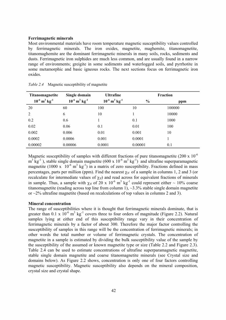
42

Ferrimagnetic minerals Most environmental materials have room temperature magnetic susceptibility values controlled by ferrimagnetic minerals. The iron oxides, magnetite, maghemite, titanomagnetite, titanomaghemite are the dominant ferrimagnetic minerals in many soils, rocks, sediments and dusts. Ferrimagnetic iron sulphides are much less common, and are usually found in a narrow range of environments; greigite in some sediments and waterlogged soils, and pyrrhotite in some metamorphic and basic igneous rocks. The next sections focus on ferrimagnetic iron oxides. Table 2.4 Magnetic susceptibility of magnetite Titanomagnetite Single domain Ultrafine Fraction

10-6 m3 kg-1 10-6 m3 kg-1 10-6 m3 kg-1 % ppm 20 60 100 10 100000 2 6 10 1 10000 0.2 0.6 1 0.1 1000 0.02 0.06 0.1 0.01 100 0.002 0.006 0.01 0.001 10 0.0002 0.0006 0.001 0.0001 1 0.00002 0.00006 0.0001 0.00001 0.1 Magnetic susceptibility of samples with different fractions of pure titanomagnetite (200 x 10-6 m3 kg-1 ), stable single domain magnetite (600 x 10-6 m3 kg-1) and ultrafine superparamagnetic magnetite (1000 x 10-6 m3 kg-1) in a matrix of zero susceptibility. Fractions defined in mass percentages, parts per million (ppm). Find the nearest χlf of a sample in columns 1, 2 and 3 (or recalculate for intermediate values of χlf) and read across for equivalent fractions of minerals in sample. Thus, a sample with χlf of 20 x 10-6 m3 kg-1 could represent either ~ 10% coarse titanomagnetite (reading across top line from column 1), ~3.3% stable single domain magnetite or ~2% ultrafine magnetite (based on recalculations of top values in columns 2 and 3). Mineral concentration The range of susceptibilities where it is thought that ferrimagnetic minerals dominate, that is greater than 0.1 x 10-6 m3 kg-1 covers three to four orders of magnitude (Figure 2.2). Natural samples lying at either end of this susceptibility range vary in their concentration of ferrimagnetic minerals by a factor of about 300. Therefore the major factor controlling the susceptibility of samples in this range will be the concentration of ferrimagnetic minerals; in other words the total number or volume of ferrimagnetic crystals. The concentration of magnetite in a sample is estimated by dividing the bulk susceptibility value of the sample by the susceptibility of the assumed or known magnetite type or size (Table 2.2 and Figure 2.3). Table 2.4 can be used to estimate concentrations of ultrafine superparamagnetic magnetite, stable single domain magnetite and coarse titanomagnetite minerals (see Crystal size and domains below). As Figure 2.2 shows, concentration is only one of four factors controlling magnetic susceptibility. Magnetic susceptibility also depends on the mineral composition, crystal size and crystal shape.

43

Mineral composition The composition of ferrimagnetic iron oxides varies from the ‘pure’ oxides of magnetite and maghemite, to ‘impure’ oxides such as titanomagnetite and titanomaghemite, in which the Fe atoms are partially substituted by atoms of titanium (Ti). There are continuous sequences or solid solutions of minerals between these two sets which have varying titanium contents. Titanium substitution reduces the Fe content and magnetic moment of the mineral, and hence lowers the magnetic susceptibility. This is confirmed in Table 2.2, which shows titanomagnetite with susceptibility values as low as 15% of the highest values for magnetite. Where titanium substitution has progressed beyond a certain point the minerals lose ferrimagnetic status and become transformed into the paramagnetic titanium oxides ilmenite and ulvospinel. The type of iron oxides which occur in specimens of igneous rock depends upon the chemical composition of the liquid magma and the mode of crystallisation. The main oxide is titanomagnetite and the proportion of titanium tends to be higher in basic rather than acid rocks. Oxidation at high temperatures (>600 °C) during cooling will result in conversion to magnetite, whilst at low temperatures (<400 °C) oxidation produces titanomaghemite. Titanomagnetites tend to form during rapid rather than slow cooling of the magma. The iron oxides will have a range of crystal dimensions from <1 μm to several millimetres, and the crystal shape can vary from spheres to rods. Weathering of igneous rocks can alter crystal structure and chemical composition, and has the crucial effect of releasing minerals into soils and sediments. The iron oxides in sedimentary rocks will in part be inherited from igneous rocks. Crystal size and domains Ferrimagnetic grains are divided up into different regions or cells of magnetisation, known as domains. Above diameters of ~110 μm, magnetite grains are referred to as multidomain (MD) because energetically it is favourable to have more than one domain. In small grains <0.2 μm, the restricted volume allows only one domain to form, and these are termed single domain (SD) grains. Grains in the interval 0.2 - 110 μm are large enough to favour more than one domain but show the magnetic properties of single domain grains; these are termed pseudo-single domain (PSD). Ultrafine grains <0.03 μm are SD but display unique properties. The magnetisation is strong but unstable due to thermal energies counteracting induced magnetisation very quickly after a magnetic field is removed. This behaviour is similar to paramagnetism, but with a much greater susceptibility. Hence it is termed superparamagnetic (SP) behaviour. Measurements on natural and synthetically produced magnetites of known sizes (Table 2.2) have helped to define the major changes in susceptibility with crystal size and domain, and these are shown in Figure 2.3. Recent measurements suggest that the variations of χlf with crystal size are smaller than previously thought and may be considered to have a constant mean of 3.1 SI (± 0.4 SI) equivalent to a χlf value of ~596 x 10-6 m3 kg-1 (± 77 x 10-6 m3 kg-1 ) over a very wide range (0.09 - 6000 μm) of crystal sizes. This range includes all the MD, PSD and stable SD domain states (SSD). In crystal diameters less than 0.03 μm, the domain state is essentially SP and values of χlf are higher and may exceed 1000 x 10-6 m3 kg-1. The SP crystals are also characterised by their response to susceptibilities measured at different frequencies and are detected by frequency dependent measurements (see below).

44

Crystal shape The crystal shape of the ferrimagnetic mineral assemblage influences magnetic susceptibility values. Longer crystals have the effect of shifting the boundaries between the domain states towards coarser crystal sizes. For example, rod-shaped crystals might exhibit SP behaviour in crystals as long as 0.05 μm. However, without other magnetic measurements or direct observations by transmission electron microscope, evaluation of the effects of crystal shape on susceptibility is difficult. In summary, where ferrimagnetic minerals dominate the magnetic mineral assemblage (i.e. κlf >0.1 x 10-6 m3 kg-1), magnetic susceptibility is controlled by the following factors in order of decreasing importance:

mineral concentration (χlf varies by factor of 200-300) mineral composition (χlf varies by factor of 3-4) crystal size (χlf varies by factor of <2) crystal shape (χlf varies by factor of <2)

Primary and secondary minerals Ferrimagnetic minerals which were formed within igneous rocks and which retain all or virtually all of their magnetic properties are referred to in this text as primary minerals. Other ferrimagnetic iron oxides and sulphides are referred to as secondary minerals; that is, they have formed by other processes that include burning, fossil fuel combustion, bacteria, soil formation, diagenesis and authigenesis. The crystal size or domain state provides a clue as to the processes of formation of magnetite. Table 2.5 shows that primary rock minerals and products of fossil fuel combustion tend to fall into MD, PSD and SSD ranges, while burning, pedogenic processes and bacterial action tend to produce fine secondary crystals of SSD or SP behaviour. Therefore, in some situations the ability to distinguish between domain and grain sizes will help to identify the process of crystal formation. However, room temperature measurements of magnetic susceptibility cannot alone distinguish between secondary or ferrimagnetic minerals and domains. The next sections therefore deal with how further measurements of frequency-dependent susceptibility, and low and high temperature susceptibility may help to identify minerals and domains.

45

Figure 2.3 Magnetic susceptibility variations with magnetite grain size; a) low frequency susceptibility showing the band of values produced by Heider et al (1996) for grains 0.09-6000 μm and values for SP/SSD grains produced by Maher (1988); b) frequency dependent susceptibility, after Maher 1988.

0.01 0.1 1 10 100 1000

4

8

12

16

20

0.01 0.1 1 10 100 1000

400

600

800

1000

1200

SP SSD PSD MD

(a)

596 77+-

χ 10

m

kg

lf-6

3-1

χ 10

m

kg

fd-6

3-1

χ % fd

Grain size (mm)

χ 10 m kg

χ %fd

fd-6 3

46

Table 2.5 Origins of magnetite/maghemite and greigite with domain size

MD PSD SSD SP Primary Magnetite/titanomagnetite x x (x) (x) Secondary Fuel combustion x x (x) (x) Pedogenesis (x) x x Bacterial magnetosomes (x) x (x) Dissimilatory bacterial magnetite x Burning (x) x Authigenic/biogenic greigite x x

MD-multidomain, PSD-pseudo-single domain, SSD-stable single domain, SP- superparamagnetic, (x) - some evidence, but not normally expected Frequency-dependent susceptibility Superparamagnetic crystals which are smaller than ~0.03 μm have a magnetic behaviour which shows rapid change over time. When they are placed in a magnetic field, and then removed, they lose the induced magnetisation received in a very short period of time; about 1/10000th of a second. This is because the natural thermal energy in ultrafine crystals is sufficiently strong to overcome the energy induced by a magnetic field. The measurement of frequency dependent susceptibility exploits this phenomenon by measuring a sample twice, at two different magnetisation frequencies. A low frequency (0.46 kHz) measurement (the standard susceptibility measurement χlf) allows the SP crystals close to the boundary with SSD grains to contribute fully to susceptibility, whilst a high frequency measurement (4.6 kHz) does not. The higher frequency has the effect of shifting the domain boundary between SP and SSD crystals to smaller crystal sizes. Thus SP crystals close to the boundary behave like SSD grains - with a lower susceptibility value (cf. Figure 2.3a). The difference in the values of the two measurements at different frequencies indicates the presence and amount of superparamagnetic minerals. It has recently been suggested that all crystals smaller than ~0.03μm show reduced susceptibility values at the high frequency measurement but there still remains an ongoing debate about the precise physical basis for frequency-dependence. There are two possible calculations of frequency dependent susceptibility: percentage frequency dependent susceptibility (χfd %) and mass specific frequency dependent susceptibility (χfd 10-9 m3 kg-1). Maximum χfd% values are similar in theoretical calculations and in synthetic grain data, reaching 14.5-16.9 % for magnetite and 11.6-14.3 % for maghemite with values of ~10-12 % for a wide and equal distribution of SP grains (Figure 2.3b). Narrow distributions of grains <0.005 μm may have significantly reduced values.

47

Maximum values for environmental samples and soils in England and Wales are 12-14 %. In non-SP grains with diameters equal or greater than 0.03 μm the frequency dependent susceptibility is about 2 % or lower, though in theory it should be zero. The mass specific frequency dependent susceptibility ranges from ~30 x 10-6 m3 kg-1 in SSD grains to 75-160 x 10-6 m3 kg-1 in the SP range. In this experimental set, and in nature, it is unlikely that grains exist either independently of each other or in narrow size ranges of discrete grains. They will probably adhere to form clusters. It is probable, for instance, that low frequency dependent values in relatively large crystals are caused by small numbers of SP crystals attached to their surfaces. A plot of χfd% versus χlf or χfd may help to discriminate between grain-size and domain state, and may give a first order classification of magnetic properties and even sources (Table 2.5). Figure 2.4 shows some common patterns of values plotted on a bivariate χlf-χfd% scattergram. Samples dominated by relatively coarse-grained non-SP ferrimagnets from igneous rocks or combustion products show relatively high χlf but virtually zero χfd. Values of χfd% < 5% are typical for samples in which non-SP grains dominate the assemblage or where extremely fine grains (<0.005 μm) dominate the SP fraction. For samples with χfd % 10-14%, SP grains usually from soil dominate the assemblage and χfd can be used semi-quantitatively to estimate their total concentration. Samples dominated by paramagnetic or canted antiferromagnetic minerals plot close to the origin. There is at present insufficient experimental data to construct with confidence a quantitative model for interpreting χfd and χfd% in terms of absolute proportions of different grain-sizes. At present, it is prudent to interpret frequency dependence data semi-quantitatively as shown in Table 2.6. Table 2.6 Interpretation of frequency dependent susceptibility values. Where χfd % >10% use χfd (mass specific) as an estimate of SP concentration. Low χfd % < 2.0 virtually no (< 10%) SP grains Medium χfd % 2.0-10.0 admixture of SP and coarser non-SP grains, or SP grains

<0.005 μm High χfd% 10.0-14.0 virtually all (>75 %) SP grains Very high χfd % >14.0 rare values, erroneous measurement, anisotropy, weak

sample or contamination

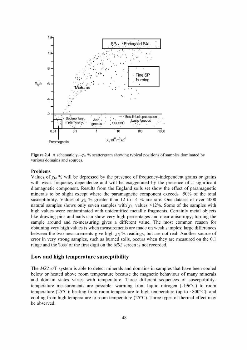
48

Figure 2.4 A schematic χlf -χfd % scattergram showing typical positions of samples dominated by various domains and sources. Problems Values of χfd % will be depressed by the presence of frequency-independent grains or grains with weak frequency-dependence and will be exaggerated by the presence of a significant diamagnetic component. Results from the England soils set show the effect of paramagnetic minerals to be slight except where the paramagnetic component exceeds 50% of the total susceptibility. Values of χfd % greater than 12 to 14 % are rare. One dataset of over 4000 natural samples shows only seven samples with χfd values >12%. Some of the samples with high values were contaminated with unidentified metallic fragments. Certainly metal objects like drawing pins and nails can show very high percentages and clear anisotropy; turning the sample around and re-measuring gives a different value. The most common reason for obtaining very high values is when measurements are made on weak samples; large differences between the two measurements give high χfd % readings, but are not real. Another source of error in very strong samples, such as burned soils, occurs when they are measured on the 0.1 range and the 'loss' of the first digit on the MS2 screen is not recorded. Low and high temperature susceptibility The MS2 κ/T system is able to detect minerals and domains in samples that have been cooled below or heated above room temperature because the magnetic behaviour of many minerals and domain states varies with temperature. Three different sequences of susceptibility-temperature measurements are possible: warming from liquid nitrogen (-196°C) to room temperature (25°C); heating from room temperature to high temperature (up to ~800°C); and cooling from high temperature to room temperature (25°C). Three types of thermal effect may be observed.

0.01 0.1 1 10 100 1000

6X %fd

X 10 m kglf-6 3 -1

4

2

8

10

12

SP Enhanced Soil

Fine SPburning

Mixtures

Sedimentarymetamorphic Acid

igneous SSD/MD

Fossil fuel combustionbasic igneous

Paramagnetic

49

Thermal disordering In simple terms, the magnetisation and hence κlf of a material is a competition between the ordering of atomic magnetic moments and their disordering by thermal energies. As a sample is heated, internal thermal energies are aided by external energy, which as a general rule causes the κlf to reduce. Paramagnetic substances show a decline in κlf with increasing temperature (°K) according to the Curie-Weiss Law (Figure 2.5). With the exception of superparamagnetic domains, ferrimagnetic and canted antiferromagnetic minerals undergo abrupt transitions at Curie (TC) and Néel (TN) temperatures respectively from magnetically ordered states below and disordered states above where they behave as paramagnetic substances (Figure 2.5). TC and TN values for common iron-bearing minerals (Table 2.7) range from +770°C to -218°C, but it should be noted that many TC and TN values are approximate and may vary according to the precise crystalline structure, degree of oxidation and presence of impurities. In superparamagnetic grains, external heat also aids the destruction of magnetisation by internal thermal energies, but cooling opposes internal thermal energies and shifts the grains towards SSD behaviour, with a lower κlf (Figure 2.5). The temperature of the transition point between SP and SSD behaviour is known as the blocking temperature (TB) which is close to room temperature for large (0.03 μm) SP magnetite crystals. Magnetocrystalline anisotropy phase transitions In addition to changes in the ordering of magnetic behaviour there are also two significant changes caused by transitions in the crystalline structure of minerals. The Verwey transition takes place in MD magnetite at about -155°C as a result of thermally activated changes to the crystal lattice structure. At this transition there is a reduction in the κlf values towards higher temperatures, the magnitude of which increases with decreasing oxidation state and large domain sizes. Pure maghemite shows no Verwey transition. The Morin transition takes place in haematite at about -10 °C as the spin-canted moment disappears giving rise to a drop in κlf at lower temperatures. The actual temperature at which the Morin transition takes place can vary widely down to temperatures as low as -90°C depending on the amount of titanium substitution and domain status. Large (MD) haematite grains and zero substitution give rise to the clearest transitions. Mineral destruction and formation Below room temperature, most of the thermal changes are reversible with little permanent change to crystal structures and magnetic states. A major disadvantage of high temperature measurements is the frequent occurrence of irreversible changes in magnetic mineralogy through oxidation, reduction and dehydration leading to the destruction of original minerals and the formation of new ones. Table 2.8 summarises the major mineral transformations and shows that they may give rise to a variety of changes in susceptibility-temperature curves. Importantly, the thermal transformation of minerals may invalidate the diagnostic use of theoretical Curie point temperatures. The nature of mineral changes may be highly unpredictable because they are often related to other properties of the sample, such as the amount of water, organic matter, and the presence and intensity of a reducing atmosphere. As a consequence, curves of κlf during cooling from high temperature are not usually diagnostic of the original room temperature minerals.

50

Figure 2.5 Schematic illustration of temperature-susceptibility relationships in paramagnetic (P), ferrimagnetic (F), canted antiferromagnetic (CA), superparamagnetic (SP) and diamagnetic (D) materials centred on the critical Curie (TC), Néel (TN) and blocking (TB) temperatures which divide the curves into ordered and disordered zones. In practice The presence of minerals and domains is detected from the shapes of the temperature-susceptibility curves and distinctive transition points. Figure 2.6 summarises the more common features in low and high temperature curves. The lack of irreversible change and the presence of several diagnostic transitions mean that low temperature curves are easier to interpret than high temperature curves. At present, interpretations are usually qualitative and there still remain ambiguous curve shapes, especially where the sample contains a mixture of minerals. It is important to bear in mind the different magnitudes of κlf for the main minerals (cf. Table 2.2) and the consequent likelihood that ferrimagnetic minerals may completely dominate the temperature curves even where other minerals are present in significant amounts. To some extent the curve shapes are additive, such that a mixture of SSD magnetite and paramagnetic minerals will produce an intermediate curve and major transitions are often found superimposed upon curves. But great care should be exercised in drawing conclusions about the identification of minerals and their relative contributions unless calibrations using known minerals and mixtures are available. There are some limitations in using liquid nitrogen for low temperature measurements. At -196°C, some TN points (eg. ilmenite) may not be reached or be

+

-

0SP

CA

F

P

P/F/CASP

T

TTT

C

NB

Mag

netic

sus

cept

ibili

ty

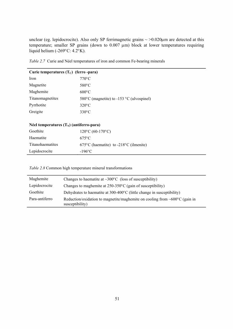
51

unclear (eg. lepidocrocite). Also only SP ferrimagnetic grains ~ >0.020μm are detected at this temperature; smaller SP grains (down to 0.007 μm) block at lower temperatures requiring liquid helium (-269°C: 4.2°K). Table 2.7 Curie and Néel temperatures of iron and common Fe-bearing minerals

Curie temperatures (TC) (ferro -para) Iron 770°C Magnetite 580°C Maghemite 600°C Titanomagnetites 580°C (magnetite) to -153 °C (ulvospinel) Pyrrhotite 320°C Greigite 330°C Néel temperatures (TN) (antiferro-para) Goethite 120°C (60-170°C) Haematite 675°C Titanohaematites 675°C (haematite) to -218°C (ilmenite) Lepidocrocite -196°C Table 2.8 Common high temperature mineral transformations

Maghemite Changes to haematite at ~300°C (loss of susceptibility) Lepidocrocite Changes to maghemite at 250-350°C (gain of susceptibility) Goethite Dehydrates to haematite at 300-400°C (little change in susceptibility) Para-antiferro Reduction/oxidation to magnetite/maghemite on cooling from ~600°C (gain in

susceptibility)

52

Figure 2.6 Schematic trends and transitions of κlf values from -196°C (liquid nitrogen) to +700°C for different minerals and domains; superparamagnetic (SP), stable single domain (SSD), multidomain (MD), paramagnetic (P), magnetite (MAG: TC 580°C), titanomagnetite (TMAG: TC 250°C); haematite (HEM). Susceptibility axis not to scale. (based on Thompson and Oldfield 1986). Weak samples In all types of studies it is possible to encounter weak samples where the room temperature susceptibility is 0.1 x 10-6 m3 kg-1 or smaller. In fact this value is large compared with the minimum repeatable κlf value on the MS2 meter of 0.1 SI units which is equivalent to ~ 0.001 x 10-6 m3 kg-1 (Part 1). Many soils, virtually all sedimentary rocks, some metamorphic and acid igneous rocks, and all samples dominated by peat or organic matter fall into this region of susceptibility (Figure 2.2). How do we interpret low susceptibility values in terms of different magnetic minerals and materials? Even at low susceptibilities magnetite crystals may be present in large quantities. Table 2.4 shows that, in the absence of other contributing minerals and materials, a value of 0.001 x 10-6 m3 kg-1 is equivalent to ~ 1 ppm of SP magnetite (0.02 μm), ~ 1.6 ppm SSD (0.2 μm) or 5 ppm titanomagnetite (20 μm). Table 2.9 shows what is meant by these figures in terms of the number of these crystals in a 10 cm3 pot where the mineral fraction represents half the pot volume; about 1 x 1012, 2 x 109 and 6 x 100 crystals respectively. At relatively low susceptibilities we may still be dealing with millions of magnetite crystals. It follows that in very weak samples with susceptibility values which cannot be measured using the MS2 system (i.e. <0.001 x 10-6 m3 kg-1), there is the danger of assuming that the sample is devoid of ferrimagnetic or paramagnetic minerals. This is not necessarily true and means that detection of very low concentrations of magnetite, such as some dusts in peat or on

SSD MD

MD HEM

TMAG

SP

P

MAG MAG

SP

TMAG

P

Tc MAG

Tc MAGParamagneticBehaviour

Ferrimagnetic mineralsformed on cooling

Morintransition

Verweytransition

Mag

netic

Sus

cept

ibilit

y

-200 -150 -100 -50 0 25 100 200 300 400 500 600 700

T C T C

Low temperature warming High temperature warming (>) and cooling (<)

53

leaves, is not possible. Nor is it correct to assume that negative susceptibility values mean that the sample is only composed of diamagnetic materials. About 45 ppm (0.0045 %) titanomagnetite or 9 ppm (0.0009 %) ultrafine magnetite is required to raise the χlf of diamagnetic peat (-0.009 x 10-6 m3 kg-1) to zero (Table 2.4). It is difficult to distinguish between very low concentrations of ferrimagnetic minerals and higher concentrations of paramagnetic or canted antiferromagnetic minerals without carrying out further magnetic analyses. Table 2.9 Numbers, volumes and total surface area of SP, SSD and MD magnetite crystals in a 10 cm3 pot of soil with bulk χlf = 0.001 . 10-6 m3 kg-1

Crystal

Diameter (μm)

Crystal Concentration

(ppm)

Crystal Volume (μm3)

Surface Area (μm2)

No. Crystals In 10 cm3 pot

Total mineral Surface area in

10 cm3 pot

SP 0.02 1 4 . 10-6 1 . 10-3 1 . 1012 1 . 109

SSD 0.2 1.6 4 . 10-3 2 . 10-1 2 . 109 3 . 108

MD 200 5 4 . 10-6 6 . 105 6 . 100 8 . 10-5

calculated assuming spherical crystals (v=4/3πr3; a=4πr2) and 50% porosity in 10 cm3 sample of soil or similar material

54

Further reading General texts Cullity, B.D. 1972 Introduction to Magnetic Materials, Addison-Wesley Publishing Company, Mass. Dunlop, D.J. and Özdemir, Ö. 1997 Rock Magnetism: fundamentals and frontiers, Cambridge University Press, Cambridge. O’Reilly, W. 1984 Rock and Mineral Magnetism, Blackie, Glasgow. Thompson, R. and Oldfield, F. 1986 Environmental Magnetism, George Allen and Unwin. Susceptibility and grain-size Heider, F., Zitelsberger, A. and Fabian, K. 1996 Magnetic susceptibility and remanent coercive force in grown magnetite crystals from 0.1 μm to 6 mm, Physics of the Earth and Planetary Interiors, 93, 239-256. Maher, B.A. 1988 Magnetic properties of some synthetic sub-micron magnetites, Geophysical Journal, 94, 83-96. Frequency-dependent susceptibility Dearing, J.A., Bird, P.M., Dann, R.J.L. and Benjamin, S.F. 1997 Secondary ferrimagnetic minerals in Welsh soils: a comparison of mineral magnetic detection methods and implications for mineral formation, Geophysical Journal International, 130, 727-736. Dearing, J.A., Dann, R.J.L., Hay, K., Lees, J.A., Loveland, P.J., Maher, B.A. and O’Grady, K. 1996 Frequency-dependent susceptibility measurements of environmental materials, Geophys. J. Int., 124, 228-240. Eyre, J.K. 1997 Frequency-dependence of magnetic susceptibility for populations of single-domain grains, Geophys. J. Int. 129, 209-211. Low and high temperature susceptibility Richter, C and van der Pluijm, B.A. 1994 Separation of paramagnetic and ferrimagnetic susceptibilities using low temperature magnetic susceptibilities and comparison with high field methods, Physics of the Earth and Planetary Interiors, 82, 113-123.

OM0409 ISSUE 7