INSTITUTE FOR THEORETICAL PHYSICS
EFT Issues and Plans
Michael Rauch | VBSCAN year 1 mid-term meeting, 07 Feb 2018
www.kit.eduKIT – University of the State of Baden-Wuerttemberg andNational Research Center of the Helmholtz Association

EFT progress in WG1
TWiki
EFT Report 1https://twiki.cern.ch/twiki/bin/view/VBSCan/ShortTermTopics
pre-meeting jointly with WG2 (June 2017)
Indico: https://indico.cern.ch/event/647015/
meeting in Karlsruhe after MBI (August 2017)
Indico: https://indico.cern.ch/event/652320/
EFT kickoff meeting (December 2017)
Indico: https://indico.cern.ch/event/688550/
WG1 periodic meeting (January 2018)
Indico: https://indico.cern.ch/event/689683/
M. Rauch – EFT Issues and Plans VBSCAN year 1 mid-term meeting, 07 Feb 2018 2/18

EFT progress in WG1
Discussion about various topics
parametrization for d = 6 and d = 8 operators
best ways to report data
validity of the EFT approach in the high-energy region
↔ unitarization methods
. . .
Questions from joint WG2-WG3 meeting
Which operators most interesting?
More info than inclusive aQGC limits?
Include Higgs data?
Combine 8 and 13 TeV data?
→ some personal remarks during the talk→ joint Vidyo meeting in few weeks
M. Rauch – EFT Issues and Plans VBSCAN year 1 mid-term meeting, 07 Feb 2018 3/18

First Steps
Effective Field Theory (EFT) as description of physics at higher energies
L = LSM + LEFT = LSM +∑d>4
∑i
f (d)i
Λd−4O(d)
i
→ lowest contribution from dimension-6 operators
→ define framework for d = 6
look at Monte Carlo codes and compare them
choose 1 or 2 operator sets (bases) for d = 6 (best candidates: Warsaw, HISZ)
identify the relevant operators (sizable tree-level interference with SM)select experimentally relevant VBS process (1, possibly 2)define optimal kinematic cuts for signal regions
can we neglect some contributions safely?how far can we go?↔ longitudinal / transverse polarization? identify CP?which input scheme? {α,MZ ,GF}, {MW ,MZ ,GF}, . . . ?
M. Rauch – EFT Issues and Plans VBSCAN year 1 mid-term meeting, 07 Feb 2018 4/18

Further Steps
study impact of each operator on cross section / distributions
look for selection cuts that distinguish between operators
→ reduce number of parameters / look at subsets
“divide and conquer”
analysis with multiple operators at the same time
extend to several VBS channels
. . .
M. Rauch – EFT Issues and Plans VBSCAN year 1 mid-term meeting, 07 Feb 2018 5/18

Code Comparison
several implementations available
SMEFTsim [Brivio, Jiang, Trott]
VBFNLO [MR, Zeppenfeld et al. ]
Whizard [Reuter, Song; Sekulla et al. ]
→ document codes and their features
→ compare codes and their features
→ Agreement?
→ Differences understood?
M. Rauch – EFT Issues and Plans VBSCAN year 1 mid-term meeting, 07 Feb 2018 6/18

The SMEFTsim package
an UFO & FeynRules model with˚: Brivio,Jiang,Trott 1709.06492feynrules.irmp.ucl.ac.be/wiki/SMEFT
1. the complete B-conserving Warsaw basis for 3 generations ,
including all complex phases and✟✟CP terms
2. automatic field redefinitions to have canonical kinetic terms
3. automatic parameter shifts due to the choice of an inputparameters set
Main scope:
estimate tree-level |ASM
A˚d“6| interference Ñ th. accuracy „ %
˚ at the moment only LO, unitary gauge implementation
[Ilaria]

The SMEFTsim package
6 different frameworks implemented Brivio,Jiang,Trott 1709.06492
③ flavorstructures
$&%
generalUp3q5 symmetriclinear MFV
ˆ ② inputschemes
#αem, mZ , Gf
mW , mZ , Gf
in 2 independent, equivalent models sets (A, B) for debugging & validation
feynrules.irmp.ucl.ac.be/wiki/SMEFT
[Ilaria]
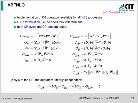
VBFNLO
[MR, Zeppenfeld, et al. ]
Implementation of D6 operators available for all VBS processesHISZ formulation, i.e. no operators with fermionsboth CP-even and CP-odd operators:
OWWW = Tr[Wµ
νWνρWρ
µ
]OWWW = Tr
[Wµ
νWνρWρ
µ
]OW = (DµΦ)† Wµν (DνΦ) OW = (DµΦ)† Wµν (DνΦ)
OB = (DµΦ)† Bµν (DνΦ) OB = (DµΦ)† Bµν (DνΦ)
OWW = Φ†WµνWµνΦ OWW = Φ†WµνWµνΦ
OBB = Φ†Bµν BµνΦ OBB = Φ†Bµν BµνΦ
OBW = Φ†BµνWµνΦ
ODW = Tr[[Dµ, Wνρ][Dµ, Wνρ]
](only 5 of the CP-odd operators linearly independent:
OBW = −2OB −OBB = −2OW −OWW )
M. Rauch – EFT Issues and Plans VBSCAN year 1 mid-term meeting, 07 Feb 2018 9/18

VBFNLO
[MR, Zeppenfeld, et al. ]
Implementation of D6 operators available for all VBS processes
HISZ formulation, i.e. no operators with fermions
both CP-even and CP-odd operators
unitarization via dipole form factor
F =
(1 +
m2inv,
∑`
Λ2
)−p
minv,∑`: invariant mass of the leptons (∼ boson pair)
Λ: characteristic scale where form factor effect becomes relevantp: exponent controlling the damping
other choices easily implementable
→ studies on validity range
https://www.itp.kit.edu/vbfnlo
M. Rauch – EFT Issues and Plans VBSCAN year 1 mid-term meeting, 07 Feb 2018 10/18
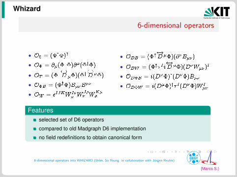
Whizard
6-dimensional operators
• O6 = (�y�)3
• O� = @�(�y�)@�(�y�)
• OT = (�y !D ��)(�y !D ��)
• O�B = (�y�)B��B��
• OW = �IJKW I�� W
J�� W
K��
• ODB = (�y !D ��)(@�B��)
• ODW = (�y� Ii !D ��)(D�W��)
I
• OD�B = i(D��)y(D��)B��
• OD�W = i(D��)y� I(D��)W I��
I Consist of Gauge bosons or Scalar field, CP-even operator
I [�] = [D�] = [Mass]1
I [B�� ] = [W�� ] = [Mass]2 in natural unit
6-dimensional operators into WHIZARD (Shim, So Young in collaboration with Jurgen Reuter)
[Marco S.]
Featuresselected set of D6 operators
compared to old Madgraph D6 implementation
no field redefinitions to obtain canonical form
Code Comparison
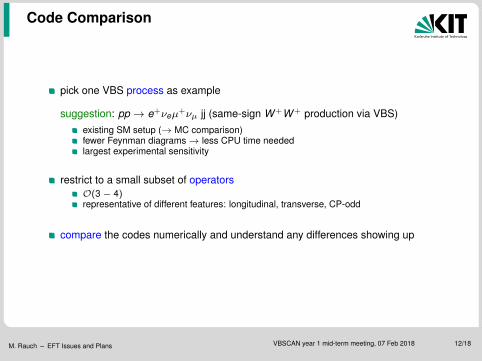
pick one VBS process as example
suggestion: pp → e+νeµ+νµ jj (same-sign W +W + production via VBS)existing SM setup (→ MC comparison)fewer Feynman diagrams→ less CPU time neededlargest experimental sensitivity
restrict to a small subset of operatorsO(3− 4)representative of different features: longitudinal, transverse, CP-odd
compare the codes numerically and understand any differences showing up
M. Rauch – EFT Issues and Plans VBSCAN year 1 mid-term meeting, 07 Feb 2018 12/18

Impact of Current LimitsInvestigate impact of D6 vs D8 operators on VBS
D6 input: Global Higgs and Gauge analysis of run-I data[Butter, Eboli, Gonzalez-Fraile, Gonzalez-Garcia, Plehn, MR]
Take results and apply to vector-boson scattering
⇒ No contribution from OGG and fermionic operators
fx/Λ2[TeV−2] LHC–Higgs + LHC–TGV + LEP–TGVBest fit 95% CL interval
fWW −0.1 (−3.1, 3.7)fBB 0.9 (−3.3, 6.1)fW 1.7 (−0.98, 5.0)fB 1.7 (−11.8, 8.8)fWWW -0.06 (−2.6, 2.6)fφ,2 1.3 (−7.2, 7.5)
For simplicity: use pos. and neg. 95% CL bound with other parameters set to zero→ slightly larger effect than true 95% CL bound
Additionally:effect from dimension-8 operator OS,1
using CMS, W±W±jj ,√
S = 8 TeV, no unitarization [arXiv:1410.6315]
fS,1/Λ4 ∈ (−118, 120)TeV−4 (for fS,0/Λ4 = 0)
M. Rauch – EFT Issues and Plans VBSCAN year 1 mid-term meeting, 07 Feb 2018 13/18

ResultsProcess: pp → W +W +jj → `+ν`+νjj ,
√S = 13 TeV, VBF cuts, NLO QCD
0.0001
0.001
0.01
0.1
0 500 1000 1500 2000
dσ/d
m4l
[fb/
bin
(20
GeV
)]
m4l [GeV]
fW=[-0.98;5.0]/TeV2
fWW=[-3.1;3.7]/TeV2
fWWW=[-2.6;2.6]/TeV2
fB=[-11.8;8.8]/TeV2
fBB=[-3.3;6.1]/TeV2
fS1=[-118;120]/TeV4
fS1=[-118;120]/TeV4+K-matrixSM
last bin: overflow bin, m4` > 2000 GeVeffect of D6 contributions in general small; largest one by OWWW
D8 operator dominating
M. Rauch – EFT Issues and Plans VBSCAN year 1 mid-term meeting, 07 Feb 2018 14/18

ResultsProcess: pp → W +W +jj → `+ν`+νjj ,
√S = 13 TeV, VBF cuts, NLO QCD
cross section when requiring m4` > mcut4`
0.01
0.1
1
10
0 500 1000 1500 2000
σ [f
b]
m4lcut [GeV]
fW=[-0.98;5.0]/TeV2
fWW=[-3.1;3.7]/TeV2
fWWW=[-2.6;2.6]/TeV2
fB=[-11.8;8.8]/TeV2
fBB=[-3.3;6.1]/TeV2
fS1=[-118;120]/TeV4
fS1=[-118;120]/TeV4+K-matrixSM 0
2
4
6
8
10
0 500 1000 1500 2000
σ [f
b]
m4lcut [GeV]
fW=[-0.98;5.0]/TeV2
fWW=[-3.1;3.7]/TeV2
fWWW=[-2.6;2.6]/TeV2
fB=[-11.8;8.8]/TeV2
fBB=[-3.3;6.1]/TeV2
fS1=[-118;120]/TeV4
fS1=[-118;120]/TeV4+K-matrixSM
OWWW contribution large only for very high m4` ↔ low event counts
excess of 10 events for m4` > 1 TeV, L = 100 fb−1, SM contrib. of 10 eventsother D6 operators below 1 event
OS1 yielding large excess even without cuts on m4`
excess of almost 500 events for m4` > 1 TeV, L = 100 fb−1
even after unitarization excess of 37 events
M. Rauch – EFT Issues and Plans VBSCAN year 1 mid-term meeting, 07 Feb 2018 15/18

Unitarization
Anomalous gauge couplings spoil cancellation↔ effects can become large→ unitarity violation→ unphysical
Several solutions:
consider only unitarity-conserving phase-space regionsloses some information→ possibly reduced sensitivitycut on relevant region might not be directly accessible (m4` vs. neutrinos)
(dipole) form factor multiplying amplitudes
F(s) =1(
1 + sΛ2
FF
)n Λ2FF, n: free parameters
K -/T -matrix unitarization [Alboteanu, Kilian, Reuter, Sekulla]
based on partial-wave analysis [Jacob, Wick]
project amplitude back onto Argand circle
M. Rauch – EFT Issues and Plans VBSCAN year 1 mid-term meeting, 07 Feb 2018 16/18
0
0.2
0.4
0.6
0.8
1
0 500 1000 1500 2000
√s [GeV]
Re(a000)
Re(a^ 000)Im(a^ 000)|a^ 000-i/2|
-0.4
-0.2
0
0.2
0.4
0.6
0 500 1000 1500 2000
Re
(a0 0
0)
√s [GeV]
SM (EV)SManom. coupl.
K-matrixform factorFF p=4
Re(a)
Im(a)
12
i2
kj
aj

Effect on Operators[Perez, Sekulla, Zeppenfeld]
[G. Perez]
take recent CMS 13 TeV W +W +jj analysis
re-interpret cross section in highest m`` bin
non-unitarized:experimental bounds from high mass range→ probing unitarity-violating region
T-matrix unitarization:significantly lower cross section↔ need to increase parameter to get same xs↔ probing different energy range
→ differential information definitely helpful
M. Rauch – EFT Issues and Plans VBSCAN year 1 mid-term meeting, 07 Feb 2018 17/18

Summary
Comparison of different EFT codes
SMEFTsim [Brivio, Jiang, Trott]VBFNLO [MR, Zeppenfeld et al. ]Whizard [Reuter, Song; Sekulla et al. ]
pick single process
restrict to small subset of operators
→ timeline: 3-6 months
pheno studies
We are open to suggestions for other codes!
M. Rauch – EFT Issues and Plans VBSCAN year 1 mid-term meeting, 07 Feb 2018 18/18

Backup
Backup
M. Rauch – EFT Issues and Plans VBSCAN year 1 mid-term meeting, 07 Feb 2018 19/18

Form of the Operators
linear EFT:
SU(3)c × SU(2)L × U(1)Y as conserved gauge groups[Buchmuller, Wyler; Hagiwara et al; Grzadkowski et al; . . . ]
building blocks:
Higgs field Φ
covariant derivative Dµ (→ ∂µ when acting on singlets)
field strength tensors Gµν , Wµν , Bµν
fermion fields ψ
⇒ construct all combinations which are
Lorentz-invariant
invariant under the gauge groups
hermitian
M. Rauch – EFT Issues and Plans VBSCAN year 1 mid-term meeting, 07 Feb 2018 20/18

Form of the Operators
Example 1:
OWW = Φ†WµνWµνΦ
12OφW =
12
Tr[WµνWµν
]Φ†Φ
lead to same contribution to Feynman rules→ equivalent
Example 2:
∂µ(
Φ†Wµν (DνΦ))
= (DµΦ)† Wµν (DνΦ) + Φ†(∂µWµν
)(DνΦ) + Φ†Wµν (DµDνΦ)
total derivative in Lagrangian gives no contribution to equations of motion
→ only two of the operators on right-hand side linearly independent
can use equations of motion to rewrite expressions
→ 59 D6 operators (2499 for flavour non-universality) [Grzadkovski et al. ]
M. Rauch – EFT Issues and Plans VBSCAN year 1 mid-term meeting, 07 Feb 2018 21/18
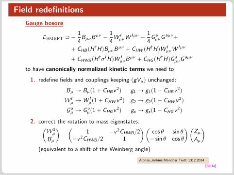
Field redefinitions
Gauge bosons
LSMEFT Ą ´ 1
4BµνB
µν ´ 1
4W IµνW
Iµν ´ 1
4G aµνG
aµν`` CHBpH:HqBµνBµν ` CHW pH:HqW I
µνWIµν
` CHWBpH:σIHqW IµνB
µν ` CHG pH:HqG aµνG
aµν
to have canonically normalized kinetic terms we need to
1. redefine fields and couplings keeping pgVµq unchanged:
Bµ Ñ Bµp1 ` CHBv2q g1 Ñ g1p1 ´ CHBv
2qW Iµ Ñ W I
µp1 ` CHW v2q g2 Ñ g2p1 ´ CHW v2qGaµ Ñ G a
µp1 ` CHGv2q gs Ñ gsp1 ´ CHGv
2q2. correct the rotation to mass eigenstates:
ˆW3µ
Bµ
˙“
ˆ1 ´v2CHWB{2
´v2CHWB{2 1
˙ ˆcos θ sin θ
´ sin θ cos θ
˙ ˆZµAµ
˙
(equivalent to a shift of the Weinberg angle)
Alonso,Jenkins,Manohar,Trott 1312.2014
[Ilaria]

Field redefinitions
Higgs
LSMEFT Ą 1
2DµH
:DµH `CH˝pH:HqpH: ˝Hq `CHDpH:DµHq˚pH:DµHq
to have a canonically normalized kinetic term, in unitary gauge, we needto replace
h Ñ h
ˆ1 ` v2CH˝ ´ v2
4CHD
˙
Alonso,Jenkins,Manohar,Trott 1312.2014
[Ilaria]

Shifts from input parameters
SM case.
Parameters in the canonically normalized Lagrangian : v , g1, g2, sθ
The values can be inferred from the measurements e.g. of
tαem,mZ ,Gf u :
αem “ g1g2g 21 ` g 2
2
mZ “ g2v
2cθ
Gf “ 1?2v2
Ñ
v2 “ 1?2Gf
sin θ2 “ 1
2
˜1 ´
d1 ´ 4παem?
2Gfm2Z
¸
g1 “?4παem
cos θ
g2 “?4παem
sin θ
in the SM at tree-level κ “ κ
[Ilaria]
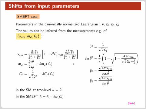
Shifts from input parameters
SMEFT case.
Parameters in the canonically normalized Lagrangian : v , g1, g2, sθ
The values can be inferred from the measurements e.g. of
tαem,mZ ,Gf u :
αem “ g1g2g 21 ` g 2
2
„1 ` v2CHWB
g 32 {g1
g 21 ` g 2
2
mZ “ g2v
2cθ` δmZ pCi q
Gf “ 1?2v2
` δGf pCi q
Ñ
v2 “ 1?2Gf
sin θ2 “ 1
2
˜1 ´
d1 ´ 4παem?
2Gfm2Z
¸
g1 “?4παem
cos θ
g2 “?4παem
sin θ
in the SM at tree-level κ “ κ
in the SMEFT κ “ κ ` δκpCiq[Ilaria]

Shifts from input parameters
To have numerical predictions it is necessary to replace κ Ñ κ ` δκpCiqfor all the parameters in the Lagrangian.
tαem,mZ ,Gf u scheme
δm2Z “ m2
Z v2
´cHD
2` 2cθsθcHWB
¯
δGf “ v2
?2
´pcp3q
Hl q11 ` pcp3qHl q22 ´ pcll q1221
¯
δg1 “ s2θ
2p1 ´ 2s2θq
˜?2δGf ` δm2
Z {m2Z ` 2
c3θ
sθcHWB v
2
¸
δg2 “ ´ c2θ
2p1 ´ 2s2θq
˜?2δGf ` δm2
Z {m2Z ` 2
s3θ
cθcHWB v
2
¸
δs2θ “ 2c2θs2θpδg1 ´ δg2q ` cθsθp1 ´ 2s2
θqcHWB v
2
δm2h “ m2
hv2
ˆ2cH˝ ´ cHD
2´ 3cH
2lam
˙
[Ilaria]

Shifts from input parameters
To have numerical predictions it is necessary to replace κ Ñ κ ` δκpCiqfor all the parameters in the Lagrangian.
tmW ,mZ ,Gf u scheme
δm2Z “ m2
Z v2
´cHD
2` 2cθsθcHWB
¯
δGf “ v2
?2
´pcp3q
Hl q11 ` pcp3qHl q22 ´ pcll q1221
¯
δg1 “ ´1
2
˜?2δGf ` 1
s2θ
δm2Z
m2Z
¸
δg2 “ ´ 1?2δGf
δs2θ “ 2c2θs2θpδg1 ´ δg2q ` cθsθp1 ´ 2s2
θqcHWB v
2
δm2h “ m2
hv2
ˆ2cH˝ ´ cHD
2´ 3cH
2lam
˙
[Ilaria]

SMEFTsim: implemented frameworks
6 different frameworks implemented:
3 flavorstructures
$’’&’’%
general
Up3q5 symmetric
linear MFV
ˆ 2 inputschemes
#αem, mZ , Gf
mW , mZ , Gf
completely general flavor indices:
2499 parameters including all complex phases
[Ilaria]

SMEFTsim: implemented frameworks
6 different frameworks implemented:
3 flavorstructures
$’’&’’%
general
Up3q5 symmetric
linear MFV
ˆ 2 inputschemes
#αem, mZ , Gf
mW , mZ , Gf
assume an exact flavor symmetry
Up3q5 “ Up3qq ˆ Up3qu ˆ Up3qd ˆ Up3ql ˆ Up3qeunder which: ψ ÞÑ Uψψ for ψ “ tu, d , q, l , eu§ The Yukawas are the only spurions breaking the symmetry:
Yu ÞÑ UuYuU:q Yd ÞÑ UdYdU
:q Yl ÞÑ UeYlU
:l .
§ flavor indices contractions are fixed by the symmetry Ñ less parameters
Examples:QHu “ pH:i
ØDµ Hqpurγµusq δrs
QeB “ BµνplrHσµνesq pYlqrs[Ilaria]

SMEFTsim: implemented frameworks
6 different frameworks implemented:
3 flavorstructures
$’’&’’%
general
Up3q5 symmetric
linear MFV
ˆ 2 inputschemes
#αem, mZ , Gf
mW , mZ , Gf
assume Up3q5 symmetry + CKM only source of✟✟CP
§ all Wilson coefficients P R§ CP odd bosonic operators are absent (9 JCP » 10´5)§ includes the first order in flavor violation expansion. E.g.:
QHu “ pH:iØDµ Hqpurγµusq
“1 ` pYuY
:uq‰
rs
Qp1qHq “ pH:i
ØDµ Hqpqrγµqsq
”1 ` pY:
uYuq ` pY:dYdq
ırs
ãÑ uLγµ
”1 ` Y :
u Yu ` VCKMY :d YdV
:CKM
ıuL
` dLγµ
”1 ` V :
CKMY :uYuVCKM ` Y :
dYd
ıdL
[Ilaria]
Recommended