
Econ 702 Macroeconomics I
Charles Engel and Menzie Chinn
Spring 2020
Lecture 23: Monetary Policy

Outline
• Recap: Why we prefer monetary policy• Discuss formally monetary policy with Taylor rule imbedded New Keynesian model• Empirical estimation of real rate

Recap

Policy Exogeneity?
•In our expositions, we have treated fiscal policy and monetary policy as being conducted in a vacuum•That is, we treat government spending and money supply changes as exogenously determined•Let’s take a look at the real world conduct of monetary policy as summarized by the policy rate – in the US the Fed funds rate

We Move Interest Rates Instead of Money Supply to Hit Full Employment Output
By choosing M in order to make (27.10) hold
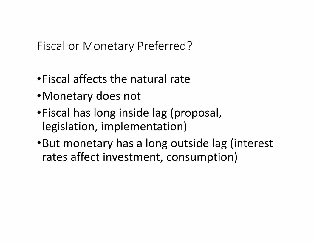
Fiscal or Monetary Preferred?
•Fiscal affects the natural rate•Monetary does not•Fiscal has long inside lag (proposal, legislation, implementation)•But monetary has a long outside lag (interest rates affect investment, consumption)

Example Why Monetary to Be Preferred
Keeping output constant by reducing G in face of positive IS shock results in r2,t < rf
1,t=> Changes composition of output at Y = Yf
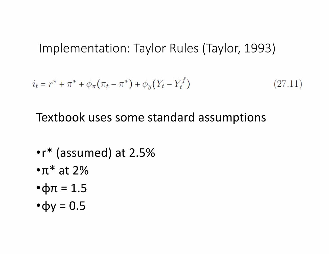
Implementation: Taylor Rules (Taylor, 1993)
Textbook uses some standard assumptions
•r* (assumed) at 2.5%•π* at 2%•φπ = 1.5 •φy = 0.5


In Reality, Central Banks “Smooth”
•One can add an autoregressive feature, letting current policy rate depend on lagged policy rate in eqn (27.11)•This will produce a better fit to the actual data •Show this using Atlanta Fed Taylor Rule apphttps://www.frbatlanta.org/cqer/research/taylor-rule

• Alt 1: Eqn 27.11 except r* = 2%
• Alt 2:Eqn 27.11, but w/smoothing parameter = 0.85
• Alt 3: Eqn27.11, except r* estimated

• Alt 1: Eqn 27.11 except r* = 2%
• Alt 2:Eqn 27.11, but w/smoothing parameter = 0.85
• Alt 3: Eqn 27.11, except r* estimated
Notice that at certain points, during the Great Recession and 2015, implied rate under Alt 1 and Alt 3 was below 0%

Replacing LM with MP CurveAppendix E

Monetary Policy Rule Closer to Reality
Modifications:•Drop money supply, demand; money stock is now in background, and endogenous•Rewrite AD, AS curves in terms of π rather than P•Replace (27.11) with (E.1)
= 0

Monetary Policy Rule Closer to Reality
Modifications:•Drop money supply, demand; money stock is now in background, and endogenous•Rewrite AD, AS curves in terms of π rather than P•Replace (27.11) with (E.1)
= 0

Monetary Policy Rule Closer to Reality
Modifications:•Drop money supply, demand; money stock is now in background, and endogenous•Rewrite AD, AS curves in terms of π rather than P•Replace (27.11) with (E.1)
= 0

Monetary Policy Rule Closer to Reality
•e has interpretation as exogenous shift term, but in policy rule•Assume:
“Adaptive expectations”

Deriving MP Curve
Subtract expected inflation from both sides (where expected inflation next period is this period’s inflation, by adaptive expectations)

Deriving the MP Curve

The Real & Financial/Monetary Sides
IS curve
MP curve
AD curve


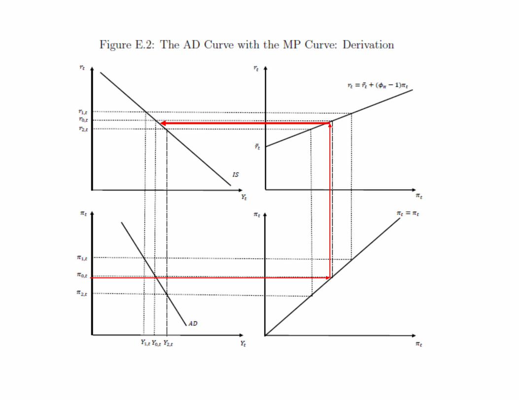

Note: this AD curve is slightly different from that in main textbook

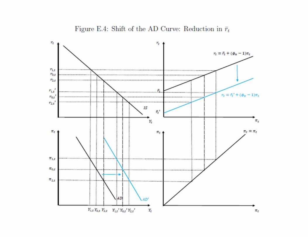
Experiments
•IS shock•Reduction in r-bar (maybe r*↓)•Changes in weight on inflation gap, φπ
•Supply shocks


Supply Side and Entire Model
Subtract Pt-1 from both sides, use approximation when P=1
Where

Expectations Augmented Phillips Curve
The rest of the supply side is essentially the same as before.


Full Model
Adaptive expectations
MP curve insteadof LM curve
Expected inflation equals change in p-bar over lagged price


Experiments
•IS shock•Increase in r-bar •Supply shocks


The Natural Rate

Empirics of Natural Rate

New Keynesian Interpretation
Where consumption equals output, and
Hamilton, et al. (2015)

Natural Rate-Growth Link Is Weak over Long Term
Hamilton, et al. (2015)

Natural Rate-Growth Link Is Weak Cross-country
Hamilton, et al. (2015)

Holston-Laubach-Williams (JIE, 2017)

Ad Hoc Empirical Approach
Hamilton, et al. (2015)

Summary
•The Natural Rate is key to implementing monetary policy•Theory (New Keynesian) implies a strong
relationship between natural rate and growth rateof potential output•The relationship is not robust in the data, either
over long spans or cross country•Most methods agree that that the natural rate has
fallen in recent years
Recommended


