ECON 1150, 2013
Functions of One Variable

ECON 1150, 2013
1. Functions of One Variable
Examples: y = 1 + 2x, y = -2 + 3x
Let x and y be 2 variables. When a unique value of y is determined by each value of x, this relation is called a function.
General form of function: y = f(x)
read “y is a function of x.”
y: Dependent variable x: Independent variable
Specific forms: y = 2 + 5x y = 80 + x2
ECON 1150, 2013
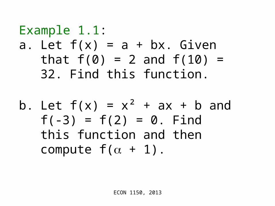
Example 1.1:a. Let f(x) = a + bx. Given that f(0) = 2
and f(10) = 32. Find this function.
b. Let f(x) = x² + ax + b and f(-3) = f(2) = 0. Find this function and then compute f( + 1).

ECON 1150, 2013
Example 1.2: Let f(x) = (x2 – 1) / (x2 + 1).
a. Find f(b/a).
b. Find f(b/a) + f(a/b).
c. f[ f(b/a) ].

ECON 1150, 2013
Domain of a function: The possible values of the independent variable x.
Range of a function: The values of the dependent variables corresponding to the values of the independent variable.
Example 1.3:
1y1- :range 1x1- :domain ,x-1 y d.
numbers real all :range 1 x:domain ,x-1 y c.
0 y :range numbers real all domain , xy .b
numbers real all range numbers real all domain ,x21y .a
2
2
y 0
0 y 1

ECON 1150, 2013
The graph of a function: The set of all points (x, f(x)).
Example 1.4:
a. Find some of the points on the graph of g(x) = 2x – 1 and sketch it.
b. Consider the function f(x) = x2 – 4x + 3. Find the values of f(x) for x = 0, 1, 2, 3, and 4. Plot these points in a xy-plane and draw a smooth curve through these points.

ECON 1150, 2013
Example 1.5: Determine the domain and range of the function
.2x1x
1y

ECON 1150, 2013
x
y
-6 -4 -2 0 2 4 6
-6
-4
-2
0
2
4
6
.2x1x
1y

ECON 1150, 2013
General form of linear functions
y = ax + b (a and b are called parameters.)
Intercept: b Slope: a
bx
y
0
a1
y = ax + b (a > 0)
Positive slope (a > 0)
b
0x
y
1
a
y = ax + b (a < 0)
Negative slope (a < 0)
1.1 Linear Functions

ECON 1150, 2013
The slope of a linear function = a
y-intercept y2 – y1 y= - ------------------ = ------------ = ------ x-intercept x2 – x1 x
Example 1.6:
a. Find the equation of the line through (-2, 3) with slope -4. Then find the y-intercept and x-intercept.
b. Find the equation of the line passing through (-1,3) and (5,-2).

ECON 1150, 2013
Example 1.7:
a. Keynesian consumption function: C = 200 + 0.6Y
Intercept = autonomous consumption = 200
Slope = MPC = 0.6
b. Demand function: Q = 600 – 6P
This function satisfies the law of demand.
ECON 1150, 2013
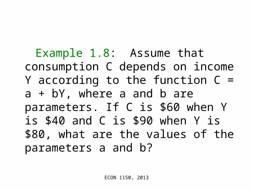
Example 1.8: Assume that consumption C depends on income Y according to the function C = a + bY, where a and b are parameters. If C is $60 when Y is $40 and C is $90 when Y is $80, what are the values of the parameters a and b?

ECON 1150, 2013
Linear functions: Constant slope
Non-linear functions: Variable slope
52.50-2.5-5
6
5.5
5
4.5
4
x
y
x
y
y = 5 + 0.2x
52.50-2.5-5
25
20
15
10
5
0
x
y
x
y
y = x2
53.752.51.250
8
7.5
7
6.5
6
x
y
x
y
y = 6 + x0.5

ECON 1150, 2013
1.2 Polynomials
34 = 3 3 3 3 = 81
(-10)3 = (-10) (-10) (-10) = - 1,000
If a is any number and n is any natural number, then the nth power of a is
an = a a … a (n times)
base: a exponent: n

ECON 1150, 2013
• an·am = an+m,
• an/am = an-m,
• (an)m = anm,
• (a·b)n = an·bn,
• (a/b)n = an/bn,
• a-n = 1 / an
• a0 = 1
General properties of exponents
For any real numbers a, b, m and n,
ECON 1150, 2013
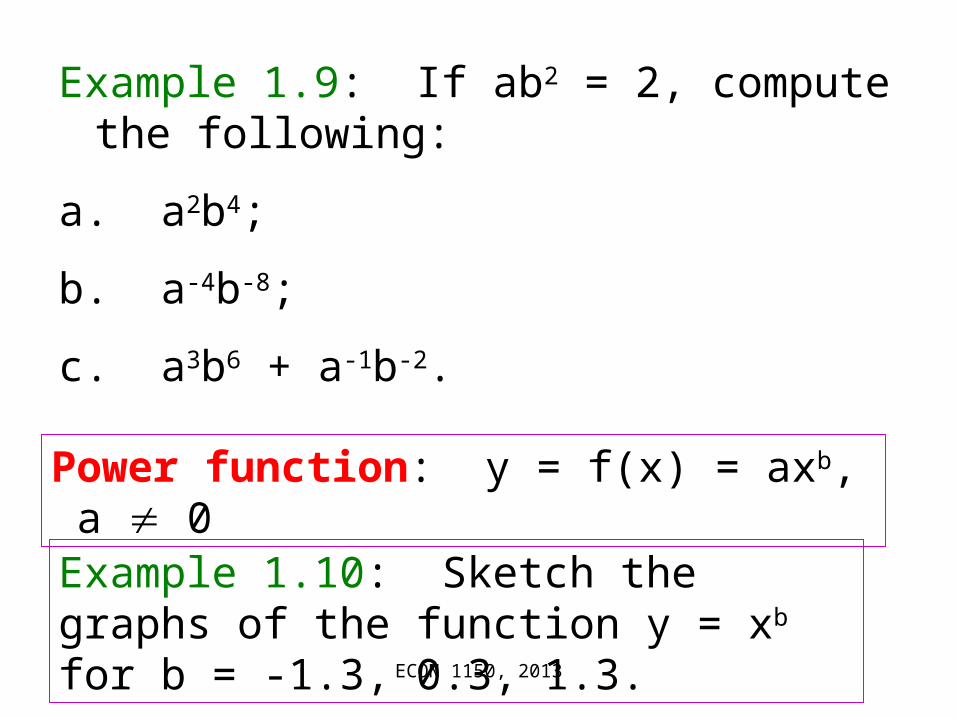
Power function: y = f(x) = axb, a 0
Example 1.9: If ab2 = 2, compute the following:
a. a2b4;
b. a-4b-8;
c. a3b6 + a-1b-2.
Example 1.10: Sketch the graphs of the function y = xb for b = -1.3, 0.3, 1.3.

ECON 1150, 2013
Linear functions: y = a + bx
Quadratic functions
y = ax2 + bx + c (a 0)
a > 0 The curve is U-shaped
a < 0 The curve is inverted U-shaped
Example 1.11: Sketch the graphs of the following quadratic functions: (a) y = x2 + x + 1; (b) y = -x2 + x + 2.

ECON 1150, 2013
Cubic functions
y = ax3 + bx2 + cx +d (a 0)
a > 0: The curve is inverted S-shaped.
a < 0: The curve is S-shaped.
Example 1.12: Sketch the graphs of the cubic functions:
(a) y = -x3 + 4x2 – x – 6;
(b) y = 0.5x3 – 4x2 + 2x + 2.

ECON 1150, 2013
Polynomial of degree n
y = anxn + ... + a2x2 + a1x + a0
where n is any non-negative integer and an 0.
n = 1: Linear function
n = 2: Quadratic function
n = 3: Cubic function

ECON 1150, 2013
1.3 Other Special Functions
t: Exponent a: BaseThe exponent is a variable.
Exponential function: y = Abt, b > 1
Example 1.13: Let y = f(t) = 2t. Then
f(3) = 23 = 8 f(-3) = 2-3 = 1/8
f(0) = 20 = 1 f(10) = 210 = 1,024
f(t + h) = 2t+h

ECON 1150, 2013
Exponential function: y = Abt
x
y
0 0.2 0.4 0.6 0.8 1 1.2 1.4 1.6 1.8 2 2.2 2.4
1
2
3
4
y = 2^x
y = 2^0.5

ECON 1150, 2013
en
n
n
11lim718281828.2 base Natural
The Natural Exponential Function
f(t) = Aet.
Examples of natural exponential functions:
y = et; y = e3t; y = Aert
or y = exp(t); y = exp(3t); y = Aexp(rt).

ECON 1150, 2013
Two Graphs of Natural Exponential Functions
x
y
-2 -1 0 1 2
1
2
3
4
y = exy = e-x

ECON 1150, 2013
Example 1.14: Which of the following equations do not define exponential functions of x?
a. y = 3x; b. y = x2; c. y = (2)x;
d. y = xx; e. y = 1 / 2x.

ECON 1150, 2013
Logarithmic function
y = bt t = logby
Rules of logarithm
ln(ab) = lna + lnb ln(a/b) = lna – lnb
ln(xa) = alnx x = elnx
ln(1) = 0 ln(e) = 1 lnex = x
Natural logarithm y = logex = lnx
We say that t is the logarithm of t to the base of b.

ECON 1150, 2013
x
y
0 0.5 1 1.5 2 2.5 3 3.5 4 4.5
1
2
3
4y = e^x
y = lnx
y = x
Logarithmic and Exponential Functions

ECON 1150, 2013
Example 1.15: Find the value of f(x) = ln(x) for x = 1, 1/e, 4 and -6.
Example 1.16: Express the following items in terms of ln2.
a. ln4; b. ln(3(32)); c. ln(1/16).
Example 1.17: Solve the following equations for x:
a. 5e-3x = 16; b. 1.08x = 10; c. ex + 4e-x = 4.
Recommended


