ECE 650 D. van Alphen 1
ECE 650 – Lecture #1
Review:
Probability & Random Variables
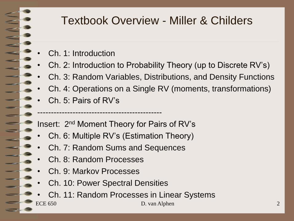
Textbook Overview - Miller & Childers
• Ch. 1: Introduction
• Ch. 2: Introduction to Probability Theory (up to Discrete RV’s)
• Ch. 3: Random Variables, Distributions, and Density Functions
• Ch. 4: Operations on a Single RV (moments, transformations)
• Ch. 5: Pairs of RV’s
----------------------------------------------
Insert: 2nd Moment Theory for Pairs of RV’s
• Ch. 6: Multiple RV’s (Estimation Theory)
• Ch. 7: Random Sums and Sequences
• Ch. 8: Random Processes
• Ch. 9: Markov Processes
• Ch. 10: Power Spectral Densities
• Ch. 11: Random Processes in Linear SystemsECE 650 D. van Alphen 2
ECE 650 D. van Alphen 3
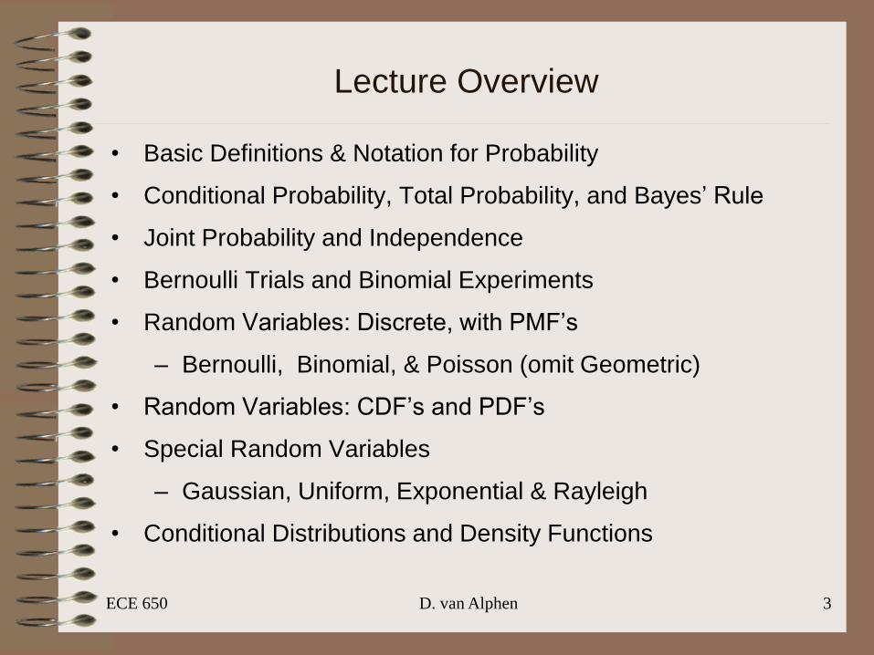
Lecture Overview
• Basic Definitions & Notation for Probability
• Conditional Probability, Total Probability, and Bayes’ Rule
• Joint Probability and Independence
• Bernoulli Trials and Binomial Experiments
• Random Variables: Discrete, with PMF’s
– Bernoulli, Binomial, & Poisson (omit Geometric)
• Random Variables: CDF’s and PDF’s
• Special Random Variables
– Gaussian, Uniform, Exponential & Rayleigh
• Conditional Distributions and Density Functions

ECE 650 D. van Alphen 4
Notation & Definition Review: Sets (Appendix A)
• Pr(A) = probability of event A
• = A-complement = S – A = {s S: s A}
• S = the sample space or the “universe”
• Review on your own: the empty set f, Venn Diagrams,
subsets, unions and intersections of sets
• Sets A and B are mutually exclusive (m.e.) if A B = f.
• {Ai} is a partition of S if
A
SA ii
fii
A
(The Ai’s “cover” S, and are pair-wise mutually exclusive (me).)

ECE 650 D. van Alphen 5
Probability Space Vocabulary Review
• S = the certain event = the set of all possible outcomes of an
experiment = the sample space = the universe
• Events: subsets of S
• Recall: if S has n elements, then it has ____ subsets.
• If zi is a single element of S, then it is called an “elementary
event”.
• The empty set or null set, f, is called the “impossible event.”
• A trial is a single performance of an experiment, with single
outcome zi S. If zi A, then we say that event A has
occurred.
ECE 650 D. van Alphen 6
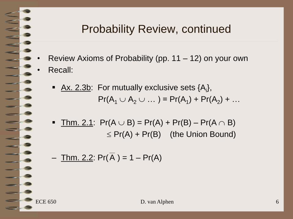
Probability Review, continued
• Review Axioms of Probability (pp. 11 – 12) on your own
• Recall:
Ax. 2.3b: For mutually exclusive sets {Ai},
Pr(A1 A2 … ) = Pr(A1) + Pr(A2) + …
Thm. 2.1: Pr(A B) = Pr(A) + Pr(B) – Pr(A B)
Pr(A) + Pr(B) (the Union Bound)
– Thm. 2.2: Pr( ) = 1 – Pr(A)A
ECE 650 D. van Alphen 7
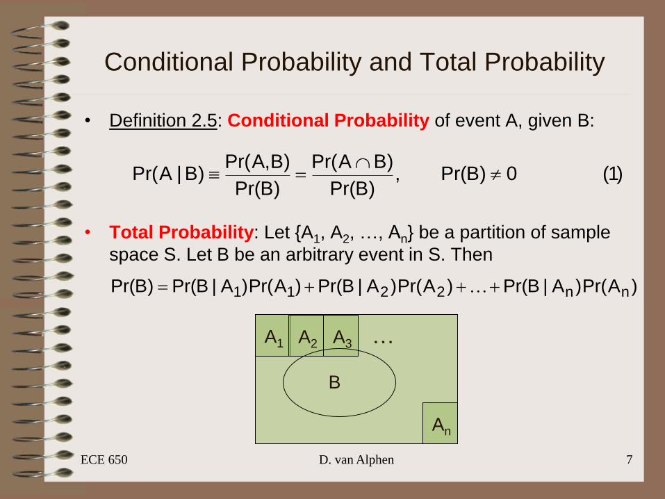
Conditional Probability and Total Probability
• Definition 2.5: Conditional Probability of event A, given B:
• Total Probability: Let {A1, A2, …, An} be a partition of sample
space S. Let B be an arbitrary event in S. Then
)1(0)BPr(,)BPr(
)BAPr(
)BPr(
)B,APr()B|APr(
)APr()A|BPr()APr()A|BPr()APr()A|BPr()BPr( nn2211
A1 A2 A3
An
…
B
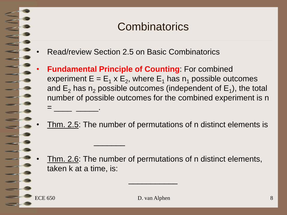
Combinatorics
• Read/review Section 2.5 on Basic Combinatorics
• Fundamental Principle of Counting: For combined
experiment E = E1 x E2, where E1 has n1 possible outcomes
and E2 has n2 possible outcomes (independent of E1), the total
number of possible outcomes for the combined experiment is n
= ____ _____.
• Thm. 2.5: The number of permutations of n distinct elements is
_______
• Thm. 2.6: The number of permutations of n distinct elements,
taken k at a time, is:
___________
ECE 650 D. van Alphen 8
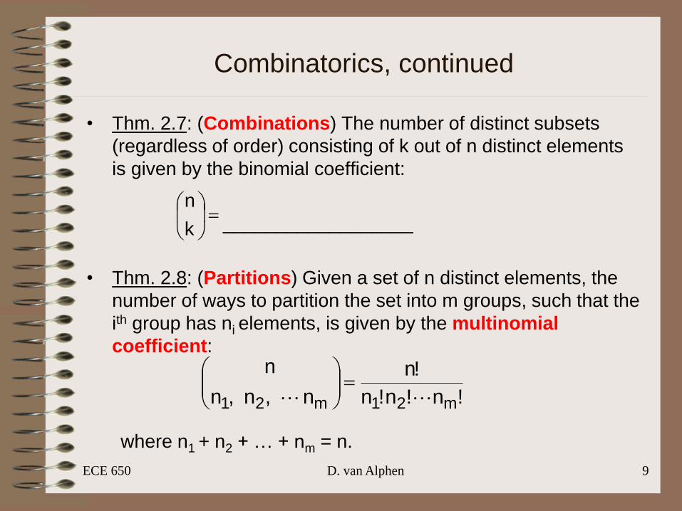
Combinatorics, continued
• Thm. 2.7: (Combinations) The number of distinct subsets
(regardless of order) consisting of k out of n distinct elements
is given by the binomial coefficient:
__________________
• Thm. 2.8: (Partitions) Given a set of n distinct elements, the
number of ways to partition the set into m groups, such that the
ith group has ni elements, is given by the multinomial
coefficient:
where n1 + n2 + … + nm = n.
ECE 650 D. van Alphen 9
k
n
!n!n!n
!n
n,n,n
n
m21m21
ECE 650 D. van Alphen 10
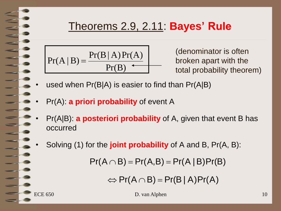
Theorems 2.9, 2.11: Bayes’ Rule
• used when Pr(B|A) is easier to find than Pr(A|B)
• Pr(A): a priori probability of event A
• Pr(A|B): a posteriori probability of A, given that event B has
occurred
• Solving (1) for the joint probability of A and B, Pr(A, B):
)APr()A|BPr()BAPr(
)BPr(
)APr()A|BPr()B|APr(
(denominator is often
broken apart with the
total probability theorem)
)BPr()B|APr()B,APr()BAPr(
ECE 650 D. van Alphen 11
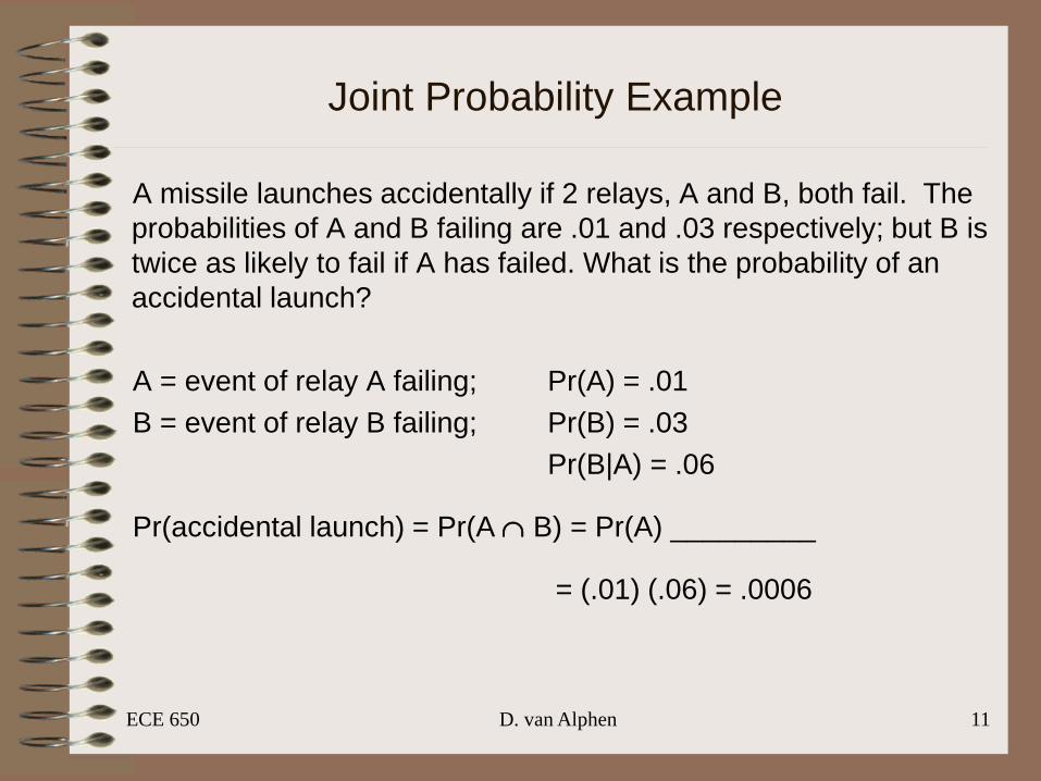
Joint Probability Example
A missile launches accidentally if 2 relays, A and B, both fail. The
probabilities of A and B failing are .01 and .03 respectively; but B is
twice as likely to fail if A has failed. What is the probability of an
accidental launch?
A = event of relay A failing; Pr(A) = .01
B = event of relay B failing; Pr(B) = .03
Pr(B|A) = .06
Pr(accidental launch) = Pr(A B) = Pr(A) _________
= (.01) (.06) = .0006
ECE 650 D. van Alphen 12
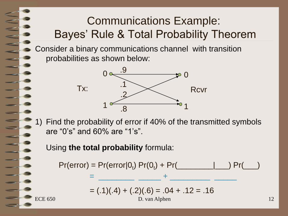
Communications Example:
Bayes’ Rule & Total Probability Theorem
Consider a binary communications channel with transition
probabilities as shown below:
1) Find the probability of error if 40% of the transmitted symbols
are “0’s” and 60% are “1’s”.
Using the total probability formula:
Tx: Rcvr
0
1
0
1
.9
.1
.2
.8
Pr(error) = Pr(error|0t) Pr(0t) + Pr(________|___) Pr(___)
= ________ _____ + _________ _____
= (.1)(.4) + (.2)(.6) = .04 + .12 = .16
ECE 650 D. van Alphen 13
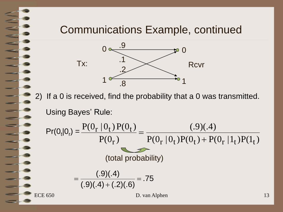
Communications Example, continued
2) If a 0 is received, find the probability that a 0 was transmitted.
Using Bayes’ Rule:
Pr(0t|0r) =
Tx: Rcvr
0
1
0
1
.9
.1
.2
.8
)1(P)1|0(P)0(P)0|0(P
)4)(.9(.
)0(P
)0(P)0|0(P
ttrttrr
ttr
(total probability)
75.)6)(.2(.)4)(.9(.
)4)(.9(.
ECE 650 D. van Alphen 14
Independent Events
• Defn 2.6: Events A and B are independent ( ) if and only if
Pr(A B) = Pr(A, B) = ________________
Pr(A | B) = ________________
Pr(B | A) = ________________
• Defn 2.7: Events A, B, and C are independent if and only if:
(i) Any pair of the three are independent; and
(ii) Pr(A, B, C) = ______ _______ ______
ECE 650 D. van Alphen 15
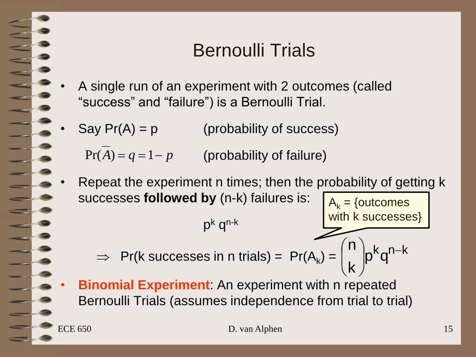
Bernoulli Trials
• A single run of an experiment with 2 outcomes (called
“success” and “failure”) is a Bernoulli Trial.
• Say Pr(A) = p (probability of success)
(probability of failure)
• Repeat the experiment n times; then the probability of getting k
successes followed by (n-k) failures is:
pk qn-k
Pr(k successes in n trials) = Pr(Ak) =
• Binomial Experiment: An experiment with n repeated
Bernoulli Trials (assumes independence from trial to trial)
pqA 1)Pr(
knkqpk
n
Ak = {outcomes
with k successes}

ECE 650 D. van Alphen 16
Binomial Experiment Example
• Five missiles are launched at a target, where each missile hits
the target with probability 0.3. Find (a) the probability that at
least one missile will hit the target, and (b) the probability that 2
missiles will hit the target.
a) Pr(at least 1 hit) = 1 – Pr(0 hits) = 1 – ________________
b) Pr(2 hits) = _______________ = 10 (.3)2 (.7)3 = .3087
= 1 - .75 = .83193
* MATLAB function: nchoosek(n, k) = nCk
ECE 650 D. van Alphen 17
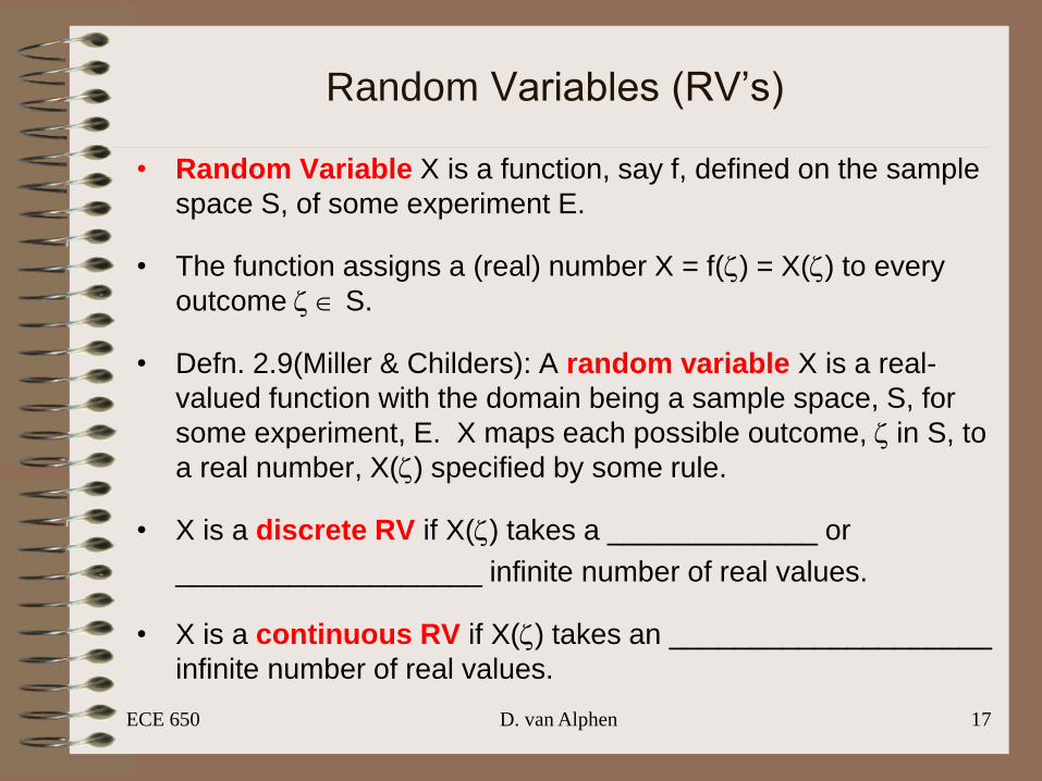
Random Variables (RV’s)
• Random Variable X is a function, say f, defined on the sample
space S, of some experiment E.
• The function assigns a (real) number X = f(z) = X(z) to every
outcome z S.
• Defn. 2.9(Miller & Childers): A random variable X is a real-
valued function with the domain being a sample space, S, for
some experiment, E. X maps each possible outcome, z in S, to
a real number, X(z) specified by some rule.
• X is a discrete RV if X(z) takes a _____________ or
___________________ infinite number of real values.
• X is a continuous RV if X(z) takes an ____________________
infinite number of real values.
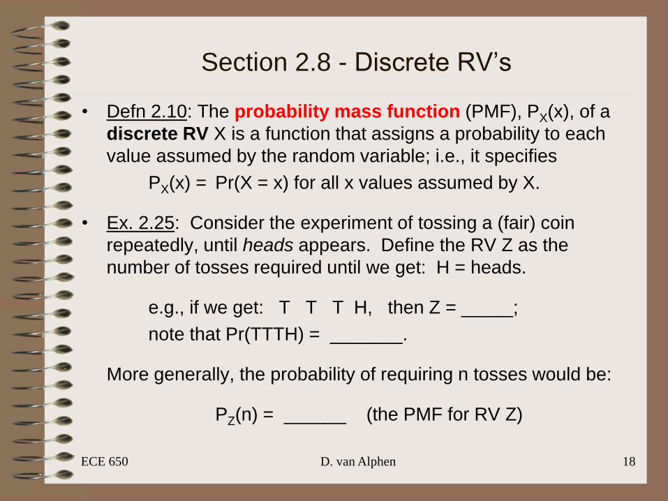
Section 2.8 - Discrete RV’s
• Defn 2.10: The probability mass function (PMF), PX(x), of a
discrete RV X is a function that assigns a probability to each
value assumed by the random variable; i.e., it specifies
PX(x) = Pr(X = x) for all x values assumed by X.
• Ex. 2.25: Consider the experiment of tossing a (fair) coin
repeatedly, until heads appears. Define the RV Z as the
number of tosses required until we get: H = heads.
e.g., if we get: T T T H, then Z = _____;
note that Pr(TTTH) = _______.
More generally, the probability of requiring n tosses would be:
PZ(n) = ______ (the PMF for RV Z)
ECE 650 D. van Alphen 18
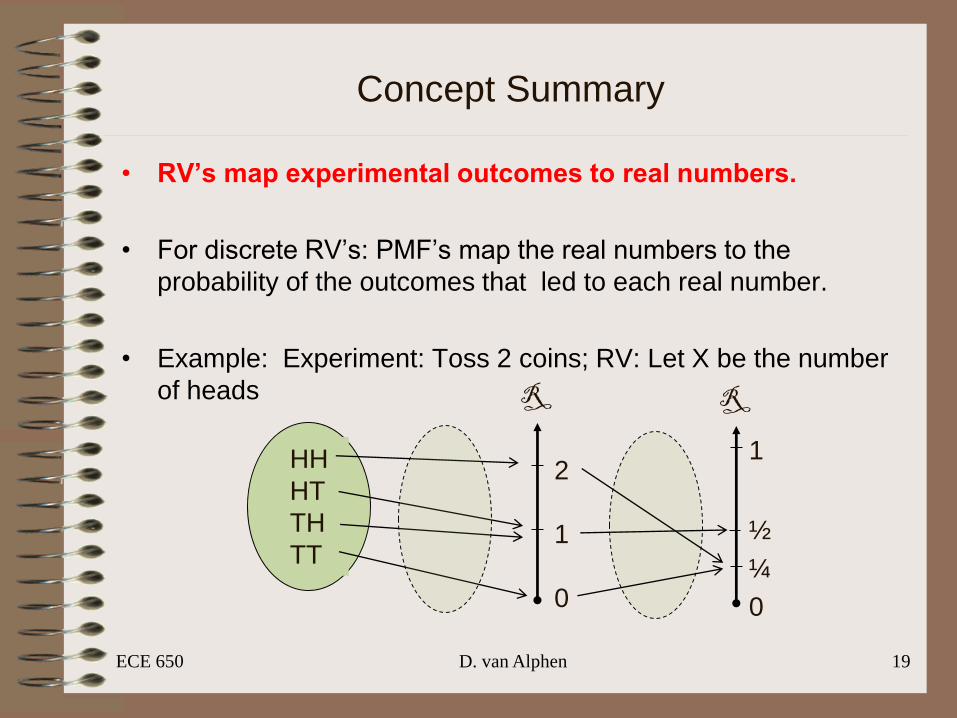
Concept Summary
• RV’s map experimental outcomes to real numbers.
• For discrete RV’s: PMF’s map the real numbers to the
probability of the outcomes that led to each real number.
• Example: Experiment: Toss 2 coins; RV: Let X be the number
of heads
ECE 650 D. van Alphen 19
HH
HT
TH
TT
R
2
1
0
R
1
½
¼
0
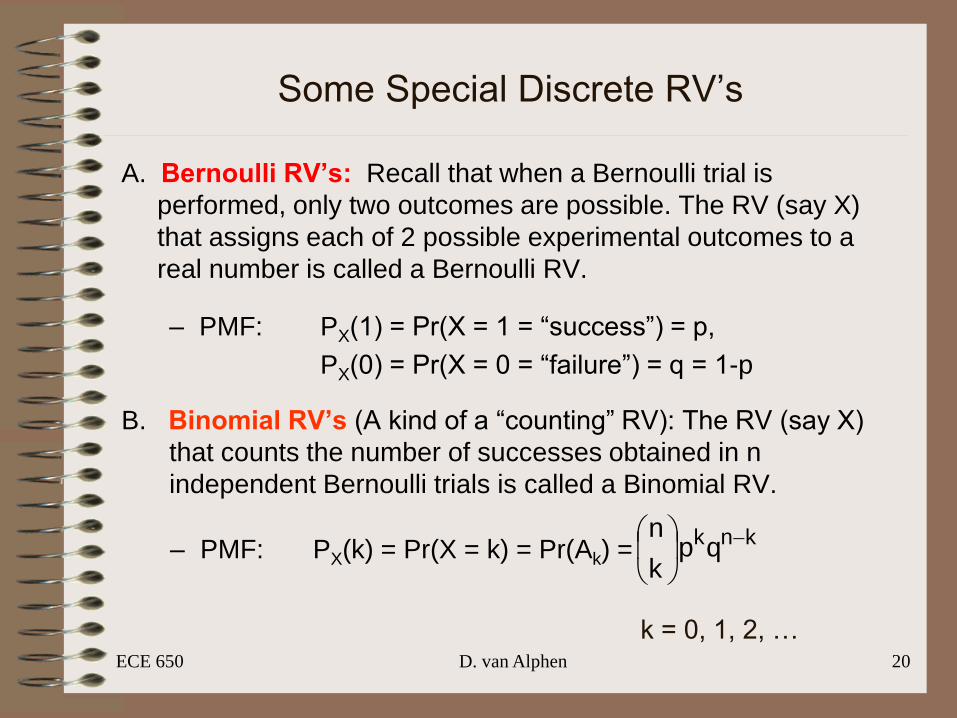
Some Special Discrete RV’s
A. Bernoulli RV’s: Recall that when a Bernoulli trial is
performed, only two outcomes are possible. The RV (say X)
that assigns each of 2 possible experimental outcomes to a
real number is called a Bernoulli RV.
– PMF: PX(1) = Pr(X = 1 = “success”) = p,
PX(0) = Pr(X = 0 = “failure”) = q = 1-p
B. Binomial RV’s (A kind of a “counting” RV): The RV (say X)
that counts the number of successes obtained in n
independent Bernoulli trials is called a Binomial RV.
– PMF: PX(k) = Pr(X = k) = Pr(Ak) =
ECE 650 D. van Alphen 20
knkqpk
n
k = 0, 1, 2, …
ECE 650 D. van Alphen 21
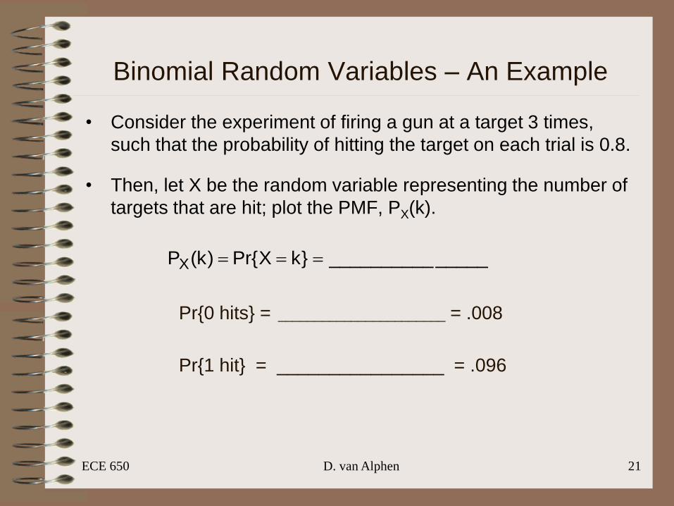
Binomial Random Variables – An Example
• Consider the experiment of firing a gun at a target 3 times,
such that the probability of hitting the target on each trial is 0.8.
• Then, let X be the random variable representing the number of
targets that are hit; plot the PMF, PX(k).
_______________}kXPr{)k(PX
Pr{0 hits} = _______________________ = .008
Pr{1 hit} = ________________ = .096
ECE 650 D. van Alphen 22
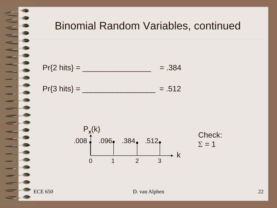
Binomial Random Variables, continued
Pr{2 hits} = ________________ = .384
Pr{3 hits} = _________________ = .512
0 1 2 3
.008 .096 .384 .512
k
Px(k)Check:
S = 1
ECE 650 D. van Alphen 23
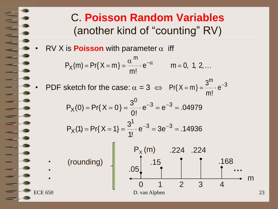
C. Poisson Random Variables
(another kind of “counting” RV)
• RV X is Poisson with parameter a iff
• PDF sketch for the case: a = 3
,2,1,0me!m
}mXPr{)m(Pm
X a
a
3m
e!m
3}mXPr{
04979.ee!0
3}0XPr{)0(P 33
0
X
14936.e3e!1
3}1XPr{)1(P 33
1
X
.
.
. m
PX (m)
0 1 2 3 4
.05.15
.224 .224
.168…
(rounding)
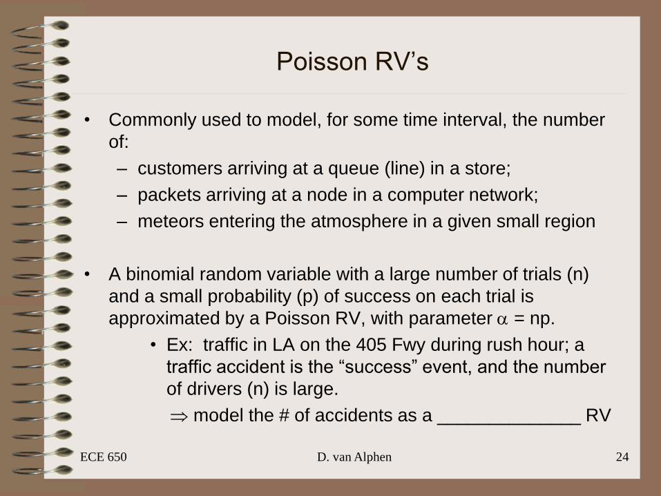
Poisson RV’s
• Commonly used to model, for some time interval, the number
of:
– customers arriving at a queue (line) in a store;
– packets arriving at a node in a computer network;
– meteors entering the atmosphere in a given small region
• A binomial random variable with a large number of trials (n)
and a small probability (p) of success on each trial is
approximated by a Poisson RV, with parameter a = np.
• Ex: traffic in LA on the 405 Fwy during rush hour; a
traffic accident is the “success” event, and the number
of drivers (n) is large.
model the # of accidents as a ______________ RV
ECE 650 D. van Alphen 24
ECE 650 D. van Alphen 25
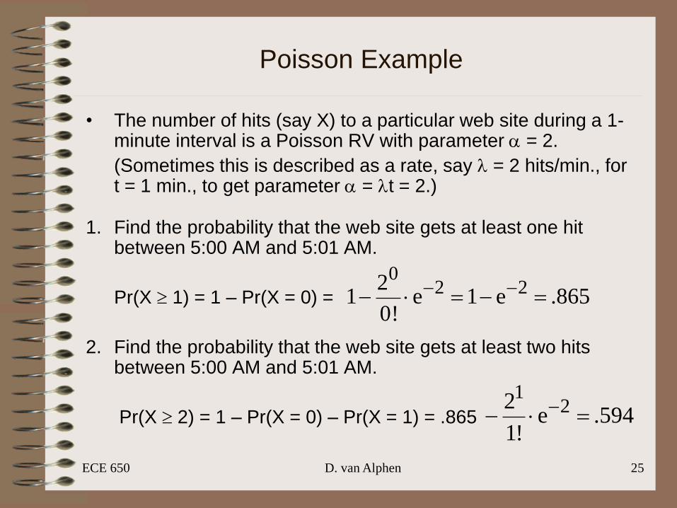
Poisson Example
• The number of hits (say X) to a particular web site during a 1-minute interval is a Poisson RV with parameter a = 2.
(Sometimes this is described as a rate, say l = 2 hits/min., for t = 1 min., to get parameter a = lt = 2.)
1. Find the probability that the web site gets at least one hit between 5:00 AM and 5:01 AM.
Pr(X 1) = 1 – Pr(X = 0) =
2. Find the probability that the web site gets at least two hits between 5:00 AM and 5:01 AM.
Pr(X 2) = 1 – Pr(X = 0) – Pr(X = 1) = .865 594.e!1
2 21
865.e1e!0
21 22
0
Your Turn
• Planes arrive at a local airport at the rate of 8 planes per hour,
so that the number of arrivals during a time period of t hours is
a Poisson RV with parameter a = 8t.
Find the probability that exactly 5 planes arrive during a 1-hour
period.
ECE 650 D. van Alphen 26
End of Chapter 2 (omitted D: Geometric RV’s)
ECE 650 D. van Alphen 27
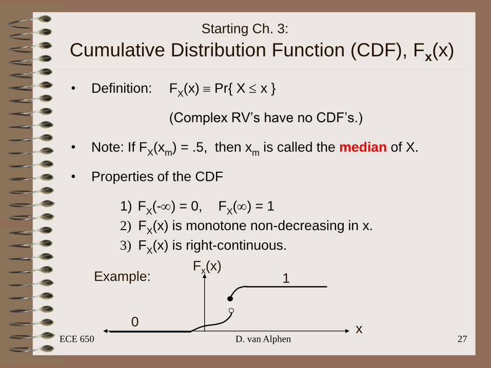
Cumulative Distribution Function (CDF), Fx(x)
• Definition: FX(x) Pr{ X x }
(Complex RV’s have no CDF’s.)
• Note: If FX(xm) = .5, then xm is called the median of X.
• Properties of the CDF
1) FX(-) = 0, FX() = 1
2) FX(x) is monotone non-decreasing in x.
3) FX(x) is right-continuous.
x
Fx(x)1
0
Example:
Starting Ch. 3:
ECE 650 D. van Alphen 28
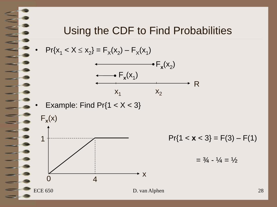
Using the CDF to Find Probabilities
• Pr{x1 < X x2} = FX(x2) – FX(x1)
• Example: Find Pr{1 < X < 3}
x2x1
R
Fx(x2)
Fx(x1)
Fx(x)
x4
1
0
Pr{1 < x < 3} = F(3) – F(1)
= ¾ - ¼ = ½
ECE 650 D. van Alphen 29
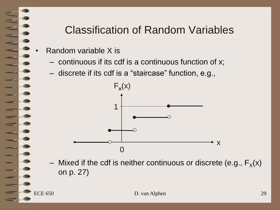
Classification of Random Variables
• Random variable X is
– continuous if its cdf is a continuous function of x;
– discrete if its cdf is a “staircase” function, e.g.,
– Mixed if the cdf is neither continuous or discrete (e.g., FX(x)
on p. 27)
Fx(x)
x
1
0
ECE 650 D. van Alphen 30
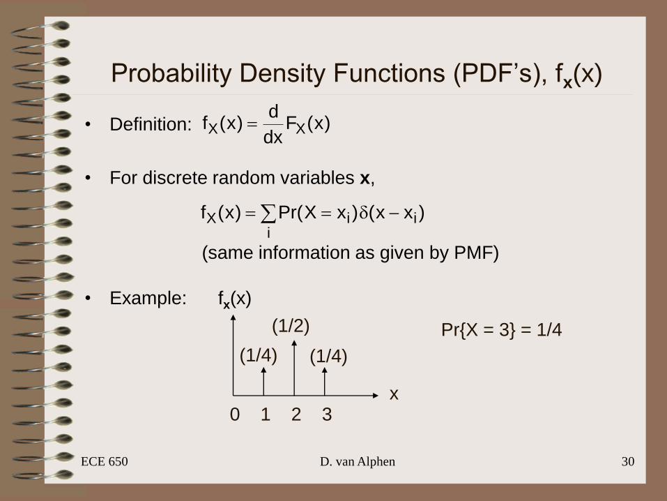
Probability Density Functions (PDF’s), fx(x)
• Definition:
• For discrete random variables x,
(same information as given by PMF)
• Example: fx(x)
)x(Fdx
d)x(f XX
)xx()xXPr()x(f ii
iX
0 1 2 3
(1/4) (1/4)
(1/2)
x
Pr{X = 3} = 1/4
ECE 650 D. van Alphen 31
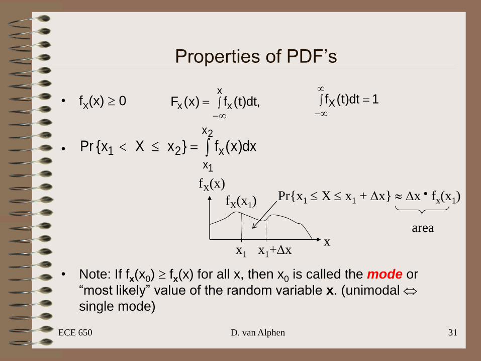
Properties of PDF’s
• fX(x) 0
•
• Note: If fx(x0) fx(x) for all x, then x0 is called the mode or
“most likely” value of the random variable x. (unimodal
single mode)
x
xx ,dt)t(f)x(F 1dt)t(fX
2
1
x
xx21 dx)x(f}xXx{Pr
fX(x)
xx1 x1+Dx
fX(x1)Pr{x1 X x1 + Dx} Dx fx(x1)
area
ECE 650 D. van Alphen 32
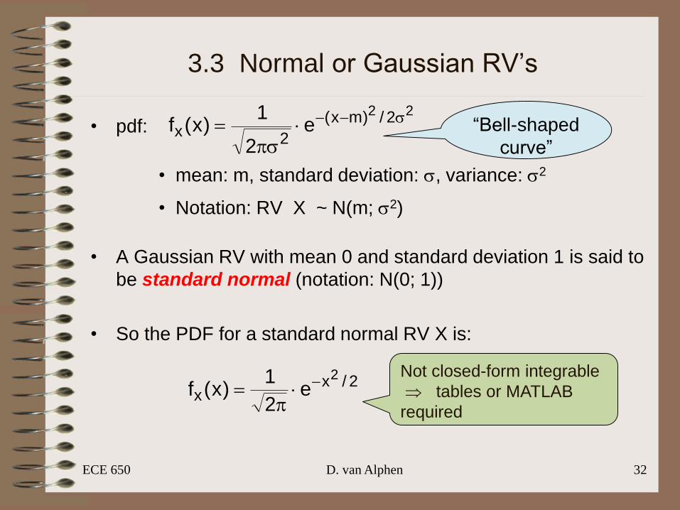
3.3 Normal or Gaussian RV’s
• pdf:
• mean: m, standard deviation: s, variance: s2
• Notation: RV X ~ N(m; s2)
• A Gaussian RV with mean 0 and standard deviation 1 is said to
be standard normal (notation: N(0; 1))
• So the PDF for a standard normal RV X is:
22 2/)mx(
2x e2
1)x(f s
s “Bell-shaped
curve”
2/xx
2e
2
1)x(f
Not closed-form integrable
tables or MATLAB
required
ECE 650 D. van Alphen 33
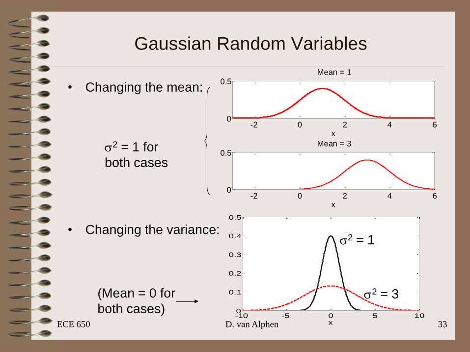
Gaussian Random Variables
• Changing the mean:
• Changing the variance:
-2 0 2 4 60
0.5
x
Mean = 1
-2 0 2 4 60
0.5
x
Mean = 3s2 = 1 for
both cases
-10 -5 0 5 100
0.1
0.2
0.3
0.4
0.5
x
s2 = 1
s2 = 3(Mean = 0 for
both cases)
ECE 650 D. van Alphen 34
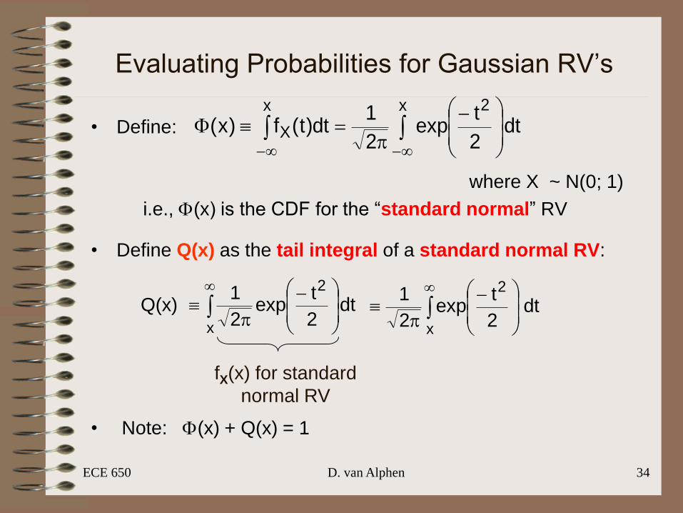
Evaluating Probabilities for Gaussian RV’s
• Define:
where X ~ N(0; 1)
i.e., F(x) is the CDF for the “standard normal” RV
• Define Q(x) as the tail integral of a standard normal RV:
Q(x)
• Note: F(x) + Q(x) = 1
F
x 2x
X dt2
texp
2
1dt)t(f)x(
dt2
texp
2
1 2
x
dt2
texp
2
1
x
2
fX(x) for standard
normal RV
D. van Alphen 35
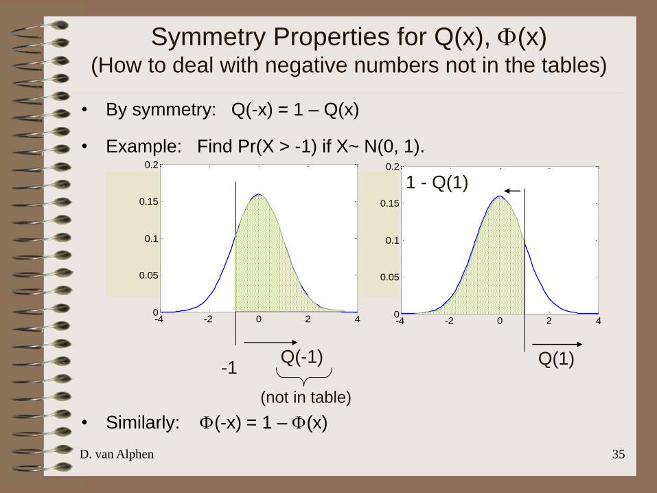
Symmetry Properties for Q(x), F(x)(How to deal with negative numbers not in the tables)
• By symmetry: Q(-x) = 1 – Q(x)
• Example: Find Pr(X > -1) if X~ N(0, 1).
• Similarly: F(-x) = 1 – F(x)
-4 -2 0 2 40
0.05
0.1
0.15
0.2
-4 -2 0 2 40
0.05
0.1
0.15
0.2
-1Q(-1) Q(1)
(not in table)
1 - Q(1)
ECE 650 D. van Alphen 36
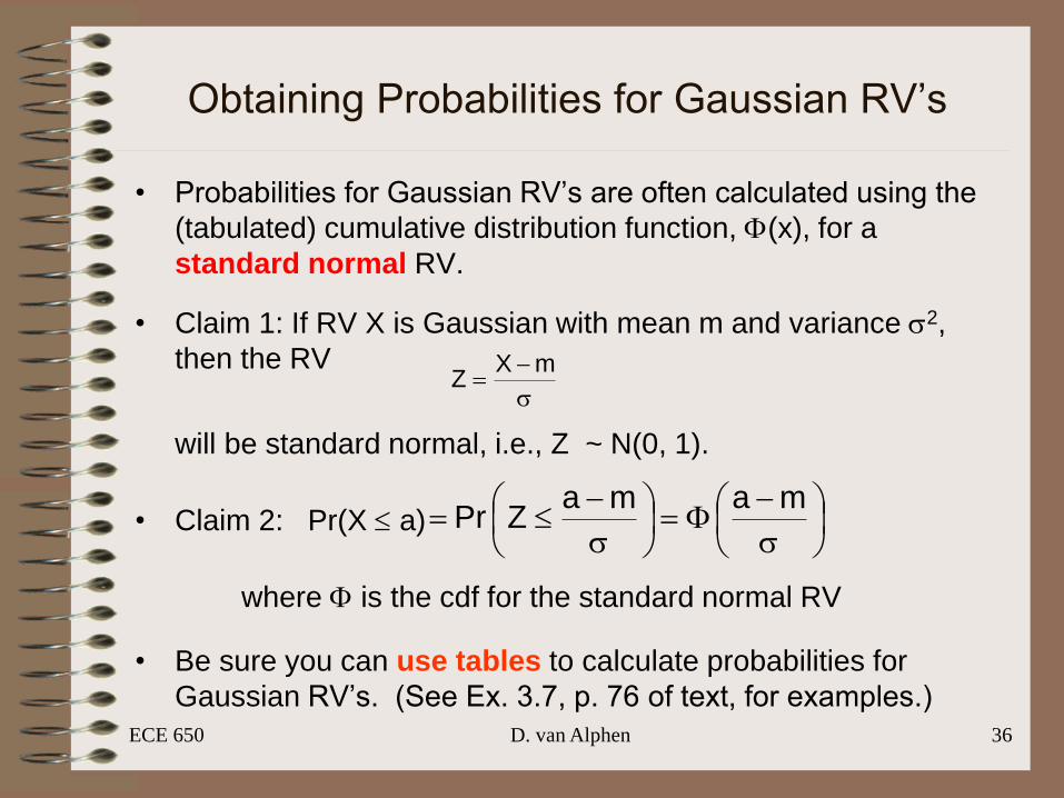
Obtaining Probabilities for Gaussian RV’s
• Probabilities for Gaussian RV’s are often calculated using the
(tabulated) cumulative distribution function, F(x), for a
standard normal RV.
• Claim 1: If RV X is Gaussian with mean m and variance s2,
then the RV
will be standard normal, i.e., Z ~ N(0, 1).
• Claim 2: Pr(X a)
where F is the cdf for the standard normal RV
• Be sure you can use tables to calculate probabilities for
Gaussian RV’s. (See Ex. 3.7, p. 76 of text, for examples.)
s
mXZ
s
F
s
mamaZPr
D. van Alphen 37
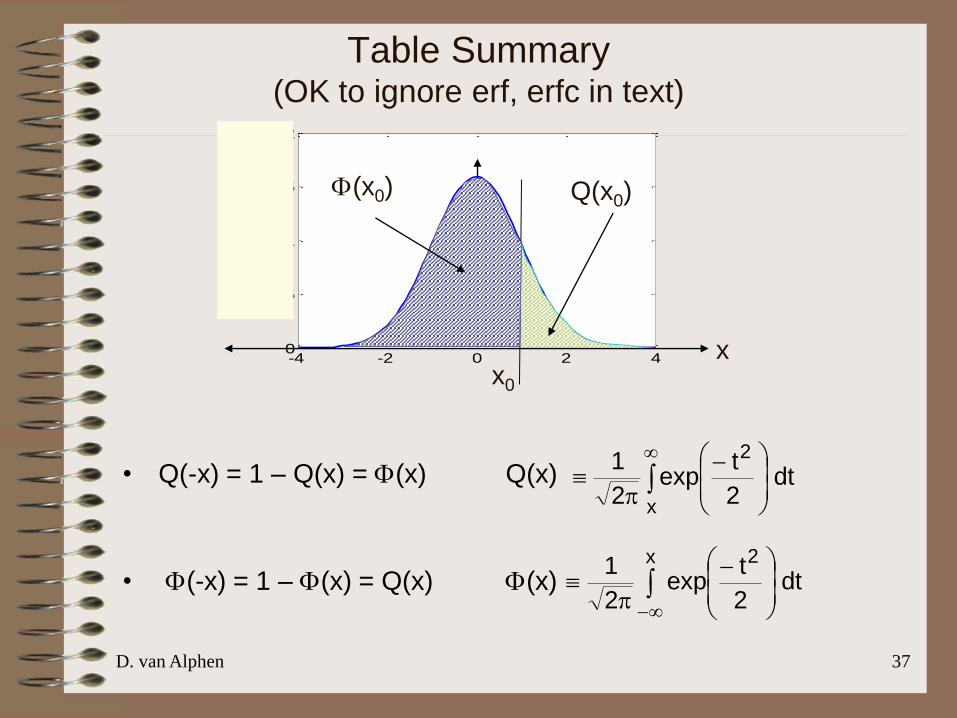
Table Summary(OK to ignore erf, erfc in text)
• Q(-x) = 1 – Q(x) = F(x) Q(x)
• F(-x) = 1 – F(x) = Q(x) F(x)
-4 -2 0 2 40
0.05
0.1
0.15
0.2
x0
x
Q(x0)F(x0)
dt2
texp
2
1
x
2
dt2
texp
2
1 x 2
ECE 650 D. van Alphen 38
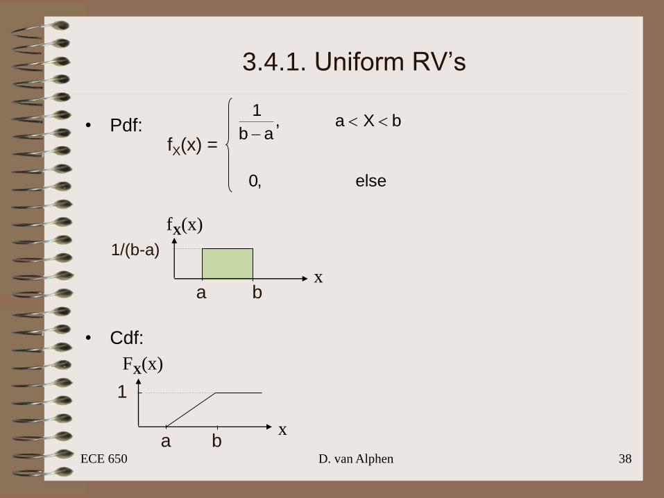
3.4.1. Uniform RV’s
• Pdf:
• Cdf:
else,0
bXa,ab
1
fX(x) =
x
FX(x)
1
a b
fX(x)
xa b
1/(b-a)
ECE 650 D. van Alphen 39
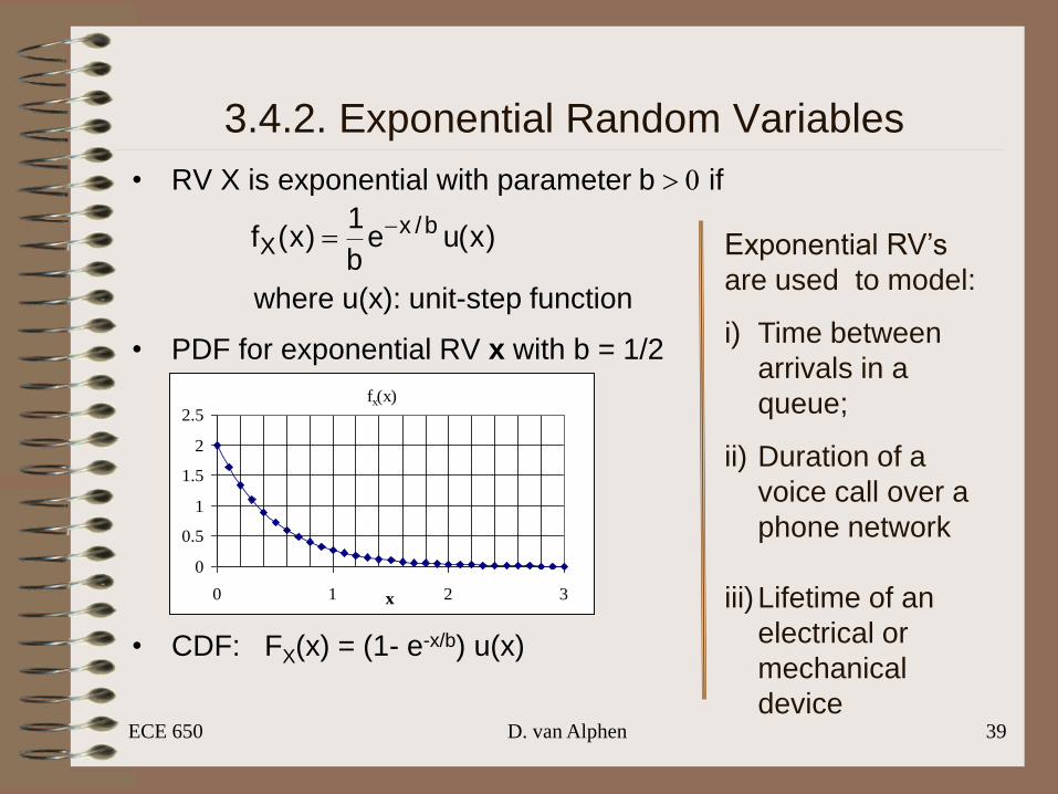
3.4.2. Exponential Random Variables
• RV X is exponential with parameter b > 0 if
where u(x): unit-step function
• PDF for exponential RV x with b = 1/2
• CDF: FX(x) = (1- e-x/b) u(x)
)x(ueb
1)x(f b/x
X
fx(x)
0
0.5
1
1.5
2
2.5
0 1 2 3x
Exponential RV’s
are used to model:
i) Time between
arrivals in a
queue;
ii) Duration of a
voice call over a
phone network
iii) Lifetime of an
electrical or
mechanical
device
ECE 650 D. van Alphen 40
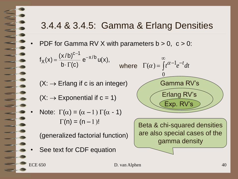
3.4.4 & 3.4.5: Gamma & Erlang Densities
• PDF for Gamma RV X with parameters b > 0, c > 0:
(X: Erlang if c is an integer)
(X: Exponential if c = 1)
• Note: G(a) = (a – 1) G(a - 1)
G(n) = (n – 1)!
(generalized factorial function)
• See text for CDF equation
),x(ue)c(b
)b/x()x(f b/x
1c
X
G
G
0
1)( dtet taawhere
Gamma RV’s
Exp. RV’s
Beta & chi-squared densities
are also special cases of the
gamma density
Erlang RV’s
D. van Alphen 41
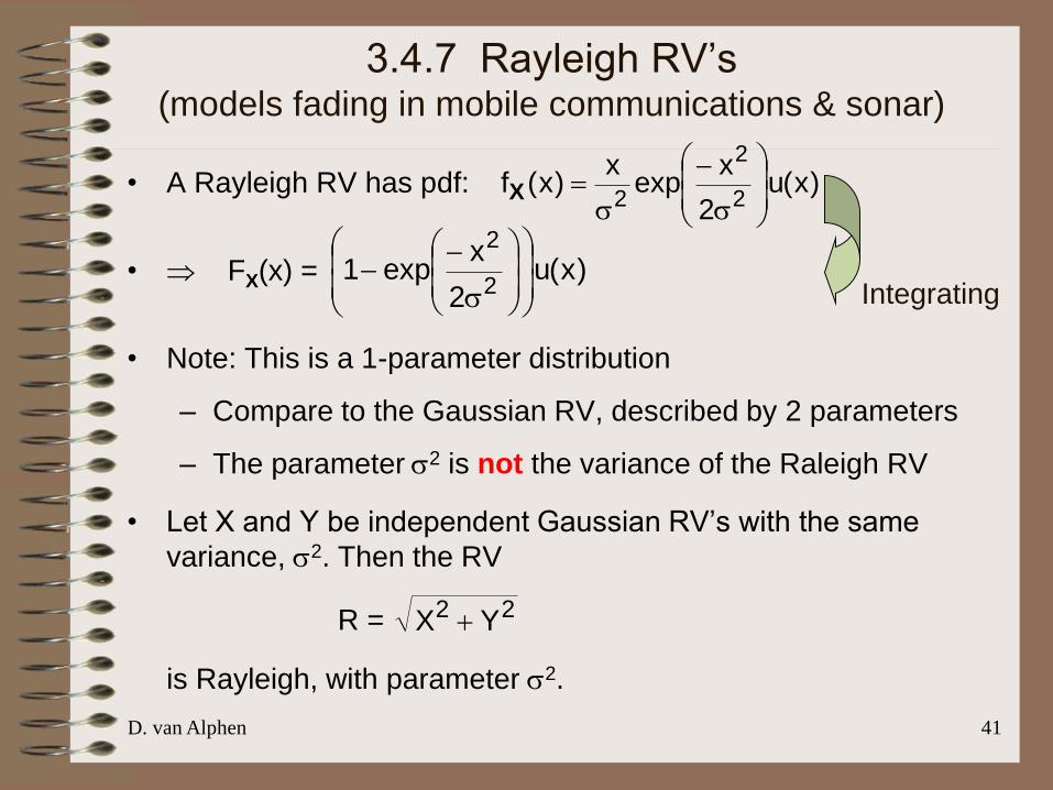
3.4.7 Rayleigh RV’s(models fading in mobile communications & sonar)
• A Rayleigh RV has pdf:
• FX(x) =
• Note: This is a 1-parameter distribution
– Compare to the Gaussian RV, described by 2 parameters
– The parameter s2 is not the variance of the Raleigh RV
• Let X and Y be independent Gaussian RV’s with the same
variance, s2. Then the RV
R =
is Rayleigh, with parameter s2.
)x(u2
xexp
x)x(f
2
2
2
s
sX
)x(u2
xexp1
2
2
s
Integrating
22 YX
D. van Alphen 42
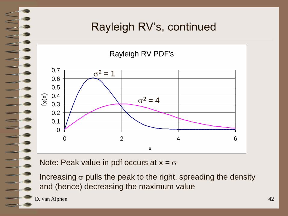
Rayleigh RV’s, continued
Rayleigh RV PDF's
0
0.1
0.2
0.3
0.4
0.5
0.6
0.7
0 2 4 6
x
f X(x
)
s2 = 4
s2 = 1
Note: Peak value in pdf occurs at x = s
Increasing s pulls the peak to the right, spreading the density
and (hence) decreasing the maximum value
ECE 650 D. van Alphen 43
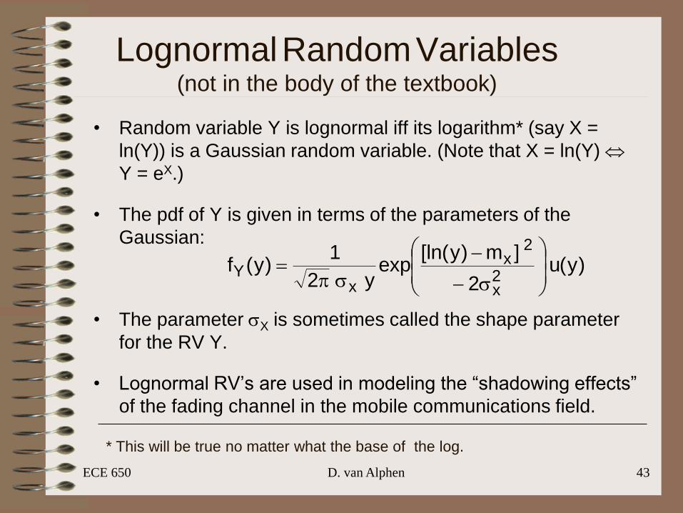
LognormalRandomVariables(not in the body of the textbook)
• Random variable Y is lognormal iff its logarithm* (say X =
ln(Y)) is a Gaussian random variable. (Note that X = ln(Y)
Y = eX.)
• The pdf of Y is given in terms of the parameters of the
Gaussian:
• The parameter sX is sometimes called the shape parameter
for the RV Y.
• Lognormal RV’s are used in modeling the “shadowing effects”
of the fading channel in the mobile communications field.
)y(u2
]m)y[ln(exp
y2
1)y(f
2x
2x
xY
s
s
* This will be true no matter what the base of the log.
ECE 650 D. van Alphen 44
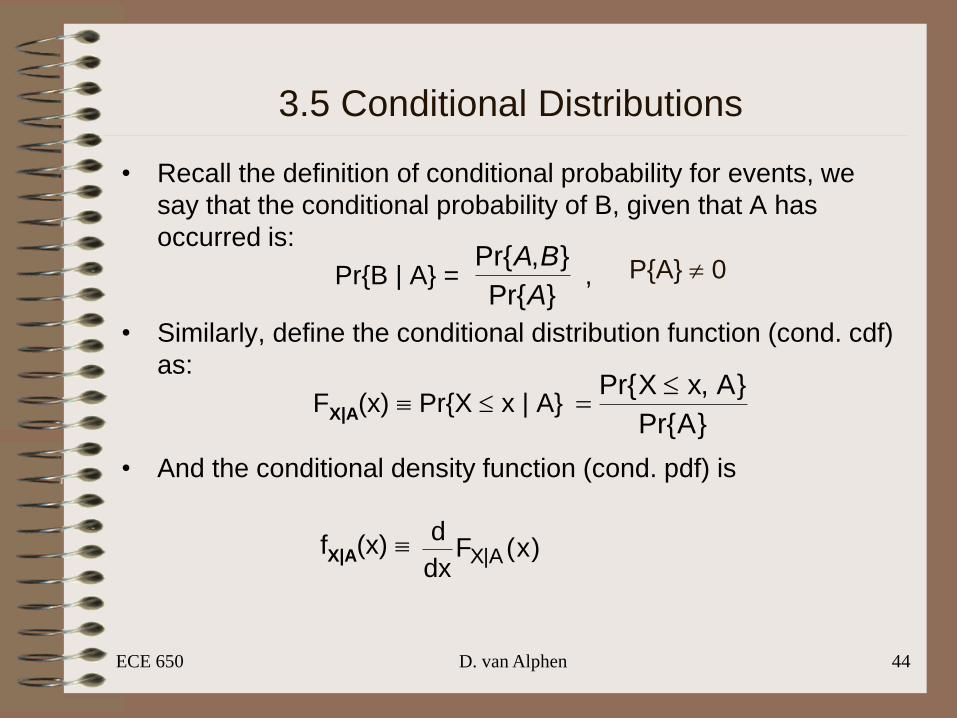
3.5 Conditional Distributions
• Recall the definition of conditional probability for events, we
say that the conditional probability of B, given that A has
occurred is:
Pr{B | A} = ,
• Similarly, define the conditional distribution function (cond. cdf)
as:
FX|A(x) Pr{X x | A}
• And the conditional density function (cond. pdf) is
fX|A(x)
}Pr{
},Pr{
A
BA
}APr{
}A,xXPr{
)x(Fdx
dA|X
P{A} 0
ECE 650 D. van Alphen 45
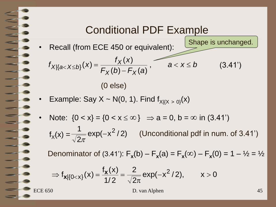
Conditional PDF Example
• Recall (from ECE 450 or equivalent):
• Example: Say X ~ N(0, 1). Find fX|{X > 0}(x)
• Note: {0 < x} = {0 < x } a = 0, b = in (3.41’)
fX(x) =
bxaaFbF
xfxf
XX
XbXaX
,
)()(
)()(}{|
(0 else)
(3.41’)
)2/xexp(2
1 2
Denominator of (3.41’): Fx(b) – Fx(a) = Fx() – Fx(0) = 1 – ½ = ½
0x),2/xexp(2
2
2/1
)x(f)x(f 2
}x0{| >
x
x
(Unconditional pdf in num. of 3.41’)
Shape is unchanged.
ECE 650 D. van Alphen 46
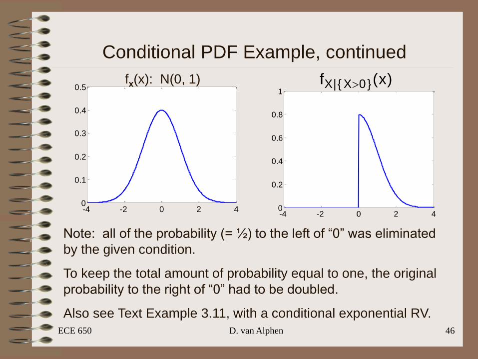
Conditional PDF Example, continued
)x(f }0X{|X >fx(x): N(0, 1)
-4 -2 0 2 40
0.2
0.4
0.6
0.8
1
-4 -2 0 2 40
0.1
0.2
0.3
0.4
0.5
Note: all of the probability (= ½) to the left of “0” was eliminated
by the given condition.
To keep the total amount of probability equal to one, the original
probability to the right of “0” had to be doubled.
Also see Text Example 3.11, with a conditional exponential RV.
ECE 650 D. van Alphen 47
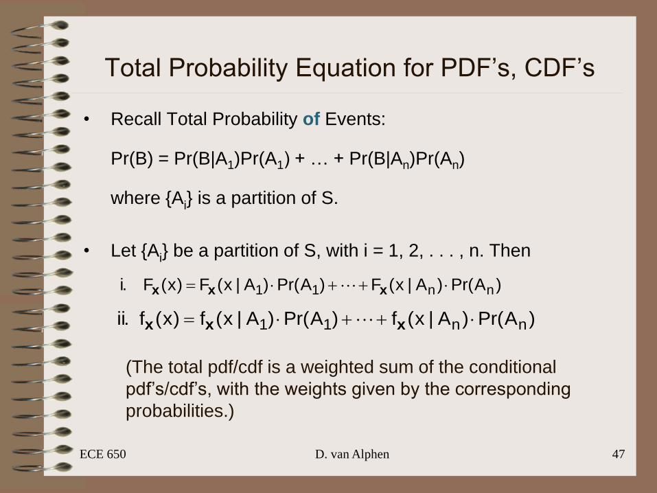
Total Probability Equation for PDF’s, CDF’s
• Recall Total Probability of Events:
Pr(B) = Pr(B|A1)Pr(A1) + … + Pr(B|An)Pr(An)
where {Ai} is a partition of S.
• Let {Ai} be a partition of S, with i = 1, 2, . . . , n. Then
)APr()A|x(F)APr()A|x(F)x(F.i nn11 xxx
)APr()A|x(f)APr()A|x(f)x(f.ii nn11 xxx
(The total pdf/cdf is a weighted sum of the conditional
pdf’s/cdf’s, with the weights given by the corresponding
probabilities.)
ECE 650 D. van Alphen 48
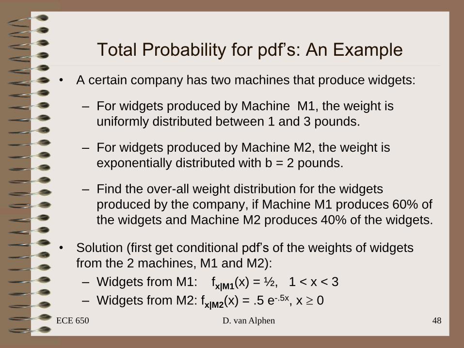
Total Probability for pdf’s: An Example
• A certain company has two machines that produce widgets:
– For widgets produced by Machine M1, the weight is
uniformly distributed between 1 and 3 pounds.
– For widgets produced by Machine M2, the weight is
exponentially distributed with b = 2 pounds.
– Find the over-all weight distribution for the widgets
produced by the company, if Machine M1 produces 60% of
the widgets and Machine M2 produces 40% of the widgets.
• Solution (first get conditional pdf’s of the weights of widgets
from the 2 machines, M1 and M2):
– Widgets from M1: fx|M1(x) = ½, 1 < x < 3
– Widgets from M2: fx|M2(x) = .5 e-.5x, x 0
ECE 650 D. van Alphen 49
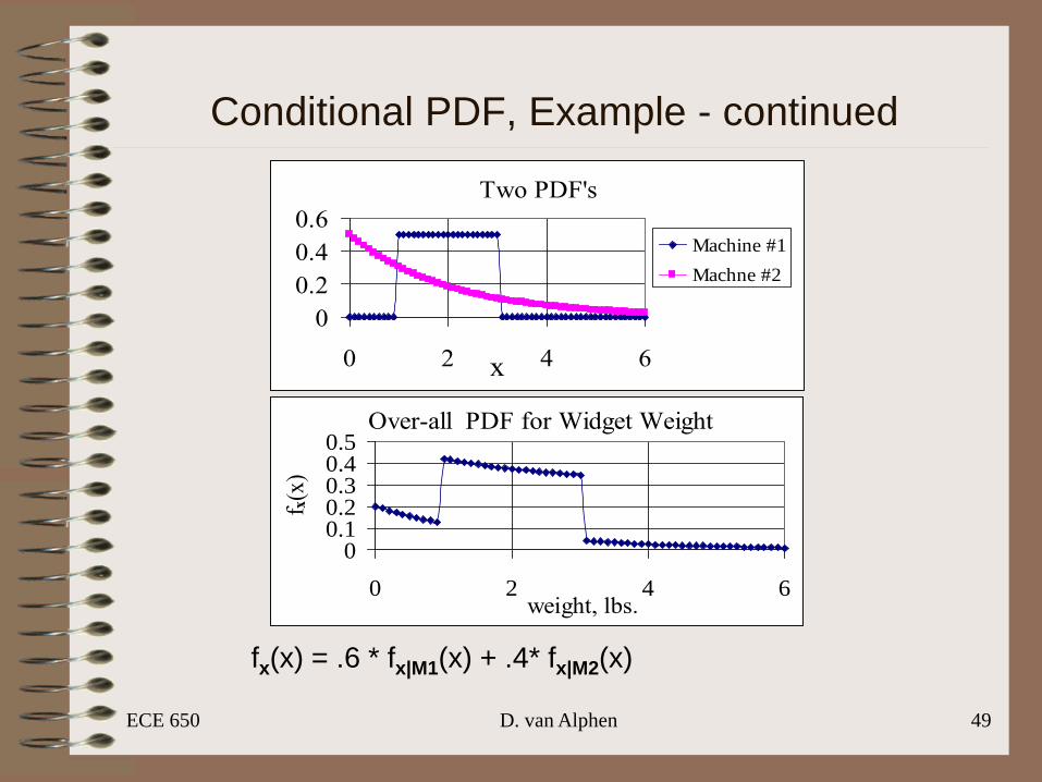
Conditional PDF, Example - continued
Two PDF's
0
0.2
0.4
0.6
0 2 4 6x
Machine #1
Machne #2
Over-all PDF for Widget Weight
00.10.20.30.40.5
0 2 4 6weight, lbs.
f x(x
)
fx(x) = .6 * fx|M1(x) + .4* fx|M2(x)
ECE 650 D. van Alphen 50
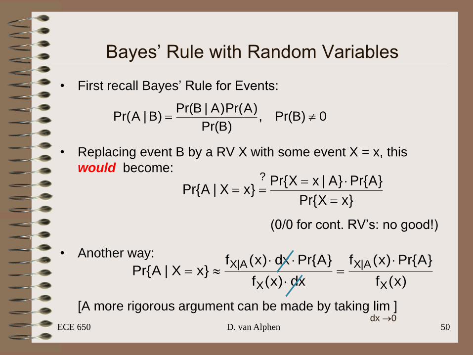
Bayes’ Rule with Random Variables
• First recall Bayes’ Rule for Events:
• Replacing event B by a RV X with some event X = x, this
would become:
(0/0 for cont. RV’s: no good!)
• Another way:
[A more rigorous argument can be made by taking lim ]
0)BPr(,)BPr(
)APr()A|BPr()B|APr(
}xXPr{
}APr{}A|xXPr{}xX|APr{
?
)x(f
}APr{)x(f
dx)x(f
}APr{dx)x(f}xX|APr{
X
A|X
X
A|X
dx 0
ECE 650 D. van Alphen 51
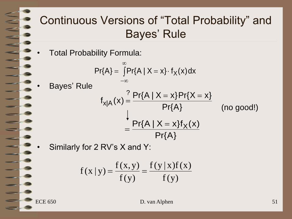
Continuous Versions of “Total Probability” and
Bayes’ Rule
• Total Probability Formula:
• Bayes’ Rule
(no good!)
• Similarly for 2 RV’s X and Y:
dx)x(f}xX|APr{}APr{ X
}APr{
}xXPr{}xX|APr{)x(f
?
A|x
}APr{
)x(f}xX|APr{ X
)y(f
)x(f)x|y(f
)y(f
)y,x(f)y|x(f
Recommended


![ECE 544 Basic Probability and Random Processesjvk/544/handouts/544...E[Xi] = .Then Pr ˆ lim n!1 X1 + + Xn n = ˙ = 1 (i.e., the sample mean converges to the true mean with probability](https://img.dokumen.tips/doc/110x75/5f6fb05d31ba6103ff72ae65/ece-544-basic-probability-and-random-processes-jvk544handouts544-exi-then.jpg)