Discussion PaPer series
IZA DP No. 10900
Arnaud DupuyAlfred Galichon
A Note on the Estimation of Job Amenities and Labor Productivity
july 2017

Any opinions expressed in this paper are those of the author(s) and not those of IZA. Research published in this series may include views on policy, but IZA takes no institutional policy positions. The IZA research network is committed to the IZA Guiding Principles of Research Integrity.The IZA Institute of Labor Economics is an independent economic research institute that conducts research in labor economics and offers evidence-based policy advice on labor market issues. Supported by the Deutsche Post Foundation, IZA runs the world’s largest network of economists, whose research aims to provide answers to the global labor market challenges of our time. Our key objective is to build bridges between academic research, policymakers and society.IZA Discussion Papers often represent preliminary work and are circulated to encourage discussion. Citation of such a paper should account for its provisional character. A revised version may be available directly from the author.
Schaumburg-Lippe-Straße 5–953113 Bonn, Germany
Phone: +49-228-3894-0Email: [email protected] www.iza.org
IZA – Institute of Labor Economics
Discussion PaPer series
IZA DP No. 10900
A Note on the Estimation of Job Amenities and Labor Productivity
july 2017
Arnaud DupuyCREA, University of Luxembourg and IZA
Alfred GalichonNew York University, Toulouse School of Economics and IZA

AbstrAct
july 2017IZA DP No. 10900
A Note on the Estimation of Job Amenities and Labor Productivity*
This note introduces a maximum likelihood estimator of the value of job amenities and
labor productivity in a single matching market based on the observation of equilibrium
matches and wages. The estimation procedure simultaneously fits both the matching
patterns and the wage curve. Our estimator is suited for applications to a wide range of
assignment problems.
JEL Classification: C35, C78, J31.
Keywords: matching, observed transfers, structural estimation, value of job amenities, value of productivity
Corresponding author:Arnaud DupuyLabour Market DepartmentLISER3, avenue de la FonteL-4364, Esch /AlzetteLuxembourg
E-mail: [email protected]
* Dupuy’s research has received funding from the FNR CORE grant C14/SC/8337045. Galichon gratefully acknowledges the support of NSF grant DMS-1716489, and ERC grants FP7-295298, FP7-312503, and FP7-337665.
2 ARNAUD DUPUY§ AND ALFRED GALICHON†
1. Introduction
Identification and estimation of both agents’ value of a match in one-to-one match-
ing models with transferable utility have been the subject of increasing interest in the
last decade. Two important applications are in the fields of family economics with the
marriage market (where the econometrician observes matching patterns, but not the
transfers) and labor economics with the labor market, or more generally the literature
on hedonic models (where the econometrician observes both the matching patterns
and the transfers).
In the case when transfers are not observed, thus in the case of the marriage
literature, Choo and Siow (2006) is a key reference which allowed to bring theoretical
models to the data. Subsequent references such as Chiappori et al. (2015), Galichon
and Salanie (2015) and Dupuy and Galichon (2014) have extended the structure of
the model in various dimensions. In particular, Dupuy and Galichon (2014) have
provided a framework for estimation of a matching model where agents match on
continuous characteristics, which they have applied to marriage market data.
In the case when transfers are observed, however, transfers may potentially pro-
vide useful supplementary information about the partners’ values of a match. In the
analysis of the labor market, for example, wages may be observed. The literature
referred to above is not very explicit on how this information may be used. Many
authors, such as Ekeland et al. (2004), Heckman et al. (2010) and Galichon and
Salanie (2015), among others, suggest techniques that implicitly or explicitly require
to perform nonparametric estimation (“hedonic regression”) of the wage curve prior
to the analysis. While this works well in the case when the relevant characteristics
is single-dimensional, as in Ekeland et al. (2004) and Heckman et al. (2010), or dis-
crete, as in Galichon and Salanie (2015), this is problematic when the characteristics
are continuous and multivariate. In this framework, Salanie (2015) shows that this
structure implies very strong testable restrictions.
ESTIMATION OF JOB AMENITIES AND LABOR PRODUCTIVITY 3
In this note, we build a flexible and tractable model of equilibrium matching and
wages on the labor market, and we show how to estimate the model using a maximum
likelihood approach. This work therefore extends our previous work, Dupuy and
Galichon (2014), to the case when transfers are observed.
Our paper is closely related to the literature on compensating wage differentials
initiated as an application of Rosen’s (1974) hedonic model to the labor market by
Lucas (1977) and Thaler and Rosen (1976), soon followed by many others; see Rosen
(1986) for an elegant presentation of the theory and a review of the early empirical
literature, and Viscusi and Aldy (2003) for a more recent review of the empirical liter-
ature. The approach in this vein consists in performing the reduced form estimation
of the wage-amenities gradient to uncover the marginal willingness of workers to pay
for or accept certain levels of (dis-)amenities at their job. A crucial assumption of this
approach is that the data contains rich enough information about a worker’s skills
to control for wage differentials due to productivity differentials across workers. For
instance, Brown (1980) proposed using panel data to estimate workers’ fixed effects
and control hence for unobserved heterogeneity whereas Garen (1988) suggested an
instrumental variable approach. Departure from this assumption implies an inherent
bias in the estimates of the compensating wage differentials, and Hwang et al. (1992)
have shown that this bias can be large. Our method contributes to this literature
by proposing a structural estimation technique to derive unbiased estimates of the
value of job amenities and productivity in a matching market where agents match on
multivariate and continuous characteristics using data about a single market.
Our model is also related to a growing empirical literature applying the celebrated
estimation technique proposed in Abowd et al. (1999) to decompose workers’ wage
differentials into differentials due to observed workers’ characteristics, unobserved
workers’ heterogeneity and firms’ heterogeneity using matched employer-employee
panel data, see among others Abowd et al. (2002), Andrews et al. (2008;2012),
Gruetter and Lalive (2009), Woodcock (2010) and Torres et al. (2013). Workers and
4 ARNAUD DUPUY§ AND ALFRED GALICHON†
firms fixed effects capture reduced form notions of workers and firms types that are
fixed over time and are identified using the mobility of workers across firms over time.
The outline for the rest of the paper is as follows. Section 2 introduces the model
and characterizes equilibrium. Section 3 presents our parametric specification of
the model and a maximum likelihood estimator on data about matches and wages.
Section 4 summarizes and concludes.
2. The model
The purpose of this section is to succinctly present our model, which is a bipartite
continuous matching model with transferable utility and logit unobserved heterogene-
ity. In our context, equilibrium transfers (wages) are observed. This is relevant for
instance in the labor market, as opposed to the marriage market where transfers are
typically unobserved. We limit ourselves to the introduction of the notation needed
for the construction of our estimator, emphasize on the additional identification and
estimation results obtained when transfers are observed and refer the interested reader
to the original paper for more details about its otherwise main properties. In the re-
mainder, to fix ideas, we use the example of the labor market where typically transfers,
in the form of wages, are observed.
2.1. Set up. Consider a one-to-one, bipartite matching model with transferable util-
ity. Assume that a worker’s characteristics are contained in a vector of attributes
x ∈ X = Rdx , while a firm’s characteristics are captured by a vector of attributes
y ∈ Y = Rdy .
Let w (x, y) be the wage of worker x when working for firm y. It is assumed that
worker x not only values her wage at firm y but also the amenities of her job at
firm y and let α (x, y) denote the value of these amenities at firm y for a worker x.
As in Dupuy and Galichon (2014), the value of amenities is further assumed to be
decomposed into a systematic value α (x, y) and a random value ε (x, y) modelled as

ESTIMATION OF JOB AMENITIES AND LABOR PRODUCTIVITY 5
Gumbel random process, whose definition is recalled in Appendix A. One therefore
has α (x, y) = α (x, y) + σ1ε (x, y) where σ1 is a scaling factor. By Proposition A.1
in that appendix, this implies that the density of probability that choosing firm y is
optimal for a worker of type x is given by
π (y|x) =exp
(α(x,y)+w(x,y)
σ1
)∫Y exp
(α(x,y′)+w(x,y′)
σ1
)dy′
(2.1)
while the expected indirect utility of worker x is
u (x) = σ1 log
∫Y
exp
(α (x, y′) + w (x, y′)
σ1
)dy′. (2.2)
Similarly, it is assumed that γ (x, y) measures the value of productivity when a
firm y matches with a worker x. This value consists of a systematic part γ (x, y)
and a random part η (x, y) modelled as a Gumbel random process, i.e. γ (x, y) =
γ (x, y)+σ2η (x, y) where σ2 is a scaling factor. A firm y employing worker x generates
therefore profits γ (x, y) − w(x, y). Under this specification, one can show that the
density of probability that choosing worker x is optimal for a firm of type y is given
by
π (x|y) =exp
(γ(x,y)−w(x,y)
σ2
)∫X exp
(γ(x′,y)−w(x′,y)
σ2
)dx′
(2.3)
while the expected indirect profits of firm y is
v (y) = σ2 log
∫X
exp
(γ (x′, y)− w (x′, y)
σ2
)dx′ (2.4)
It is assumed that there is the same mass of workers and firms, and that the workers’
types x have a density of probability f (x), and the firms’ types y have a density of
probability g (y). Therefore a feasible matching between workers and firms, which

6 ARNAUD DUPUY§ AND ALFRED GALICHON†
consists in the probability density π (x, y) of occurrence of a (x, y) pair, should have
marginal densities f and g. More formally,
M (f, g) =
{π : π (x, y) ≥ 0,
∫Yπ (x, y) dy = f (x) and
∫Xπ (x, y) dx = g (y)
}.
We now define an equilibrium on this market.
Definition 1. An equilibrium outcome (π,w) consists of an equilibrium matching
π (x, y), and an equilibrium wage w (x, y) such that:
(i) Matching π is feasible: π ∈M (f, g), and
(ii) Matching π is optimal for workers and firms given wage curve w, i.e. (2.1)
and (2.3) hold.
Note that when the scaling factors of the random values σ1 and σ2 tend to zero, the
firm’s problem and the worker’s problem converge to the deterministic maximization
problems
u (x) = maxy∈Y{α (x, y) + w (x, y)} and v (y) = max
x∈X{γ (x, y)− w (x, y)}
and the equilibrium problem consists in finding w (x, y) and π (x, y) which are com-
patible with optimality in these problems. See Remark 2.4 below.
2.2. Equilibrium Characterization. Let
φ(x, y) := α(x, y) + γ(x, y)
be the deterministic joint value of a match between a worker of type x and a firm of
type y.
Theorem 1. Under the above assumptions:
(i) The equilibrium matching π ∈M (f, g) is given by
π (x, y) = exp
(φ (x, y)− a (x)− b (y)
σ
), (2.5)
ESTIMATION OF JOB AMENITIES AND LABOR PRODUCTIVITY 7
where (a, b) normalized so that a (x0) = 0 for some x0 ∈ X is the unique solution to
the system of equations∫Y
exp
(φ (x, y)− a (x)− b (y)
σ
)dy = f (x) (2.6)∫
Xexp
(φ (x, y)− a (x)− b (y)
σ
)dx = g (y) .
(ii) The terms a and b that appear in (2.5) are related to the expected indirect
utilities u and profits v that appear in (2.2) and (2.4) by
u (x) = a (x) + σ1 log f (x) + t
v (y) = b (y) + σ2 log g (y)− t
for some t ∈ R.
(iii) The equilibrium wage w is given by
w (x, y) =σ1
σ(γ (x, y)− b (y)) +
σ2
σ(a (x)− α (x, y)) + t. (2.7)
Proof. See the Appendix.
Theorem 1 suggests a few important remarks.
Remark 2.1 (Location normalization). If a(x) and b(y) are solutions of system (2.6),
so are a(x)+t and b(y)−t. Using Equation (2.7) of Theorem 1, the equilibrium wages
are w (x, y) for the former solution and w (x, y) + t for the later. The nonuniqueness
of the solution for system (2.6) requires a normalization which is reflected in both the
constant term t appearing in the equilibrium wages equation (2.7) and the arbitrary
choice a (x0) = 0.
Remark 2.2 (Scale normalization). Equation (2.5) clearly indicates that the match-
ing probabilities are scale invariant with respect to σ, i.e. two markets otherwise
similar but one with (α, γ, σ) and one with (ασ, γσ, 1) generate the same equilibrium

8 ARNAUD DUPUY§ AND ALFRED GALICHON†
matches. However, inspection of Equation (2.7) reveals that wages are not scale in-
variant with respect to σ. While the two markets discussed above generate the same
equilibrium matches, they generate different equilibrium wages. As a results, with ob-
served wages, one can identify the scale of the systematic value of a match φ together
with the amount of heterogeneity necessary to rationalize the data. The normaliza-
tion of φ required when only matches are observed (see Dupuy and Galichon, 2014),
is not necessary when in addition wages are also observed. Interestingly enough, this
implies that both the scale of the deterministic value of a match φ and the amount of
unobserved heterogeneity necessary to rationalize the data can be compared across
markets when both matches and wages are observed in those markets.
Remark 2.3 (Identification of α and γ). The deterministic value of amenities α
and productivity γ do not appear individually in the expression of the equilibrium
matches in Equation (2.5), only the joint value of a match φ appears in this equation.
However, α and γ do appear separately in the formula of the equilibrium wages in
Equation (2.7). This clearly indicates that when only matches are observed, one
cannot identify and hence estimate the deterministic value of amenities α separately
from the deterministic value of productivity γ whereas, in contrast, if wages are
observed, one actually can identify and estimate these objects separately.
Remark 2.4 (The Becker-Shapley-Shubik model). When σ → 0, the model con-
verges to the classical model of Monge-Kantorovich, which is a continuous extension
of the model by Becker-Shapley-Shubik. Indeed, when σ1 and σ2 tend to zero, the
scaling coefficients of the random value of job amenities and productivity ε and η,
tend to zero, then the model becomes nonstochastic. Intuitively, when σ1 → 0,
the worker’s expected indirect utility u (x) tends to the deterministic indirect utility
maxy {α (x, y) + w (x, y)}, and it follows from (2.1) that the conditional choice dis-
tribution π (y|x) becomes concentrated around the optimal firm y such that u (x) =
α (x, y) + w (x, y). Similarly, when σ2 → 0, firm y’s expected indirect profits v (y)

ESTIMATION OF JOB AMENITIES AND LABOR PRODUCTIVITY 9
tends to the deterministic indirect profits maxx {γ (x, y)− w (x, y)}, and π (x|y) be-
comes concentrated around the optimal worker x such that v (y) = γ (x, y)−w (x, y).
Combining these two results, π (x, y) becomes concentrated around the set of pair
(x, y) such that u (x) + v (y) = φ (x, y), hence, in the limit when σ1 and σ2 tend to
zero, we have π ∈ M (f, g)
u (x) + v (y) ≥ φ (x, y) ∀x ∈ X , y ∈ Y
u (x) + v (y) = φ (x, y) π − a.s.
These are the classical stability conditions in the Monge-Kantorovich problem (see
Villani, 2003 and 2009), whose variants have been applied in Economics by Becker
(1973), Shapley and Shubik (1963), Gretsky, Ostroy, Zame (1992).
Remark 2.5 (The Sattinger model). Our model embeds Sattinger’s workhorse model
extensively used in the labor economics literature (see Sattinger, 1979 and 1993). This
model indeed corresponds to a matching market with no unobserved heterogeneity
(σ → 0; see Remark 2.4), unidimensional observed types (dx = dy = 1), in which
workers only care about their compensation (α = 0) and where the firm’s value of
productivity is smooth and supermodular (i.e. ∂2γ (x, y) /∂x∂y exists and is positive).
Under these restrictions, both the worker’s and firm’s problems become deterministic,
and the conditional distribution π(y|x) in this case is concentrated at one point y =
T (x), where T (x) is the only assignment of workers to firms which is nondecreasing.
The equilibrium wage w only depends on x and satisfies the differential wage equation,
namely
w′ (x) =∂γ (x, T (x))
∂x, (2.8)
and an explicit formula for the equilibrium wage is obtained by integration.

10 ARNAUD DUPUY§ AND ALFRED GALICHON†
Remark 2.6 (Continuous Mixed Logit demand). It follows from formula (2.1) that
the density of market demand for firms of type y is given by
∫X
exp(α(x,y)+w(x,y)
σ1
)∫Y exp
(α(x,y′)+w(x,y′)
σ1
)dy′
dx
which is a continuous Mixed Logit model. Likewise, the density of market demand
for workers of type x has a similar expression. The equilibrium wage w (x, y) equates
these quantities to the respective densities of supply, g(y) and f(x) respectively.
Remark 2.7 (Identification). Suppose the values of σ1 and σ2 are known, and σ1 +
σ2 = 1 for notational simplicity. Equations (2.1) and (2.3) clearly indicate that
α (x, y) + w (x, y) is identified up to a function c (x) by σ1 lnπ (x, y) + c (x), and
γ (x, y)−w (x, y) is identified up to a function d (y) by σ2 lnπ (x, y) +d (y). It follows
that α is identified up to fixed effects c (x) by
α (x, y) = σ1 lnπ (x, y)− w (x, y) + c (x) ,
while γ is identified up to fixed effects d (y) by
γ (x, y) = σ2 ln π (x, y) + w (x, y) + d (y) .
This result has been exploited in a nonparametric setting by Galichon and Salanie
(2015) and Salanie (2015). In this paper, it is exploited in a parametric setting based
on basis functions of x and y (see Section 3.3). Indeed, since α is identified up to
fixed effects c (x), the parametrization of α can only include basis functions depending
on both x and y or on y only but it cannot include basis functions depending on x
only. By a similar reasoning, the parametrization of γ cannot include basis functions
depending on y only.
ESTIMATION OF JOB AMENITIES AND LABOR PRODUCTIVITY 11
3. Parametric estimation
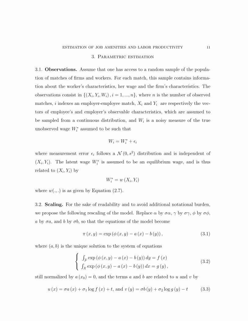
3.1. Observations. Assume that one has access to a random sample of the popula-
tion of matches of firms and workers. For each match, this sample contains informa-
tion about the worker’s characteristics, her wage and the firm’s characteristics. The
observations consist in {(Xi, Yi,Wi) , i = 1, ..., n}, where n is the number of observed
matches, i indexes an employer-employee match, Xi and Yi are respectively the vec-
tors of employee’s and employer’s observable characteristics, which are assumed to
be sampled from a continuous distribution, and Wi is a noisy measure of the true
unobserved wage W ∗i assumed to be such that
Wi = W ∗i + εi
where measurement error εi follows a N (0, s2) distribution and is independent of
(Xi, Yi). The latent wage W ∗i is assumed to be an equilibrium wage, and is thus
related to (Xi, Yi) by
W ∗i = w (Xi, Yi)
where w(., .) is as given by Equation (2.7).
3.2. Scaling. For the sake of readability and to avoid additional notational burden,
we propose the following rescaling of the model. Replace α by σα, γ by σγ, φ by σφ,
a by σa, and b by σb, so that the equations of the model become
π (x, y) = exp (φ (x, y)− a (x)− b (y)) , (3.1)
where (a, b) is the unique solution to the system of equations∫Y exp (φ (x, y)− a (x)− b (y)) dy = f (x)∫X exp (φ (x, y)− a (x)− b (y)) dx = g (y) ,
(3.2)
still normalized by a (x0) = 0, and the terms a and b are related to u and v by
u (x) = σa (x) + σ1 log f (x) + t, and v (y) = σb (y) + σ2 log g (y)− t (3.3)

12 ARNAUD DUPUY§ AND ALFRED GALICHON†
and the equilibrium wage w is given by
w (x, y) = σ1 (γ (x, y)− b (y)) + σ2 (a (x)− α (x, y)) + t. (3.4)
This scaling is without loss of generality since from Equation (3.4) one can estimate
parameters σ1 and σ2 and hence σ = σ1 +σ2 and therefore recover the pre-scaling val-
ues of α and γ. In the remainder of the paper, Equations (3.1)–(3.4) will characterize
the model to estimate.
3.3. Parametrization. Let A and Γ be two vectors of Rk parameterizing the func-
tion of workers’ systematic net value of job amenities α and the function of firms’
systematic value of productivity γ, in a linear way, so that
α(x, y;A) =K∑k=1
Akϕk(x, y), and γ(x, y; Γ) =K∑k=1
Γkϕk(x, y),
where the basis functions ϕk are linearly independent, and may include functions that
depend on x (respectively y) only. Note that by definition, the function of the joint
value of a match reads as
φ(x, y; Φ) =K∑k=1
Φkϕk(x, y), (3.5)
where Φk = Ak + Γk. Inspection of Equation (3.4) reveals that, given the parametric
choice above, equilibrium matching and wages are parameterized by (A,Γ, σ1, σ2, t).
The model is hence fully parameterized by θ = (A,Γ, σ1, σ2, t, s2), which we make
explicit by writing the predicted equilibrium wage as w(x, y; θ).
3.4. Estimation by maximum likelihood. The main purpose is to estimate the
vector of parameters θ. To this aim we adopt a maximum likelihood approach. It
follows from Remark (2.3) that the likelihood of observing a pair (x, y) only depends
on Φ = A+ Γ, and is given by
π(x, y; Φ) = exp (φ (x, y; Φ)− a(x; Φ)− b(y; Φ)) ,

ESTIMATION OF JOB AMENITIES AND LABOR PRODUCTIVITY 13
where a(x; Φ) and b(y; Φ) are uniquely determined by system of equations (3.2). Since,
by assumption, measurement errors in wages are independent of (X, Y ), the log-
likelihood of an observation (x, y, w) at parameter θ is therefore
logL (x, y, w; θ) = log π (x, y; Φ)− (w − w (x, y; θ))2
2s2− 1
2log s2,
and hence, the log likelihood of the sample reads as:
logL (θ) = nEπ
[φ (X, Y ; Φ)− a (X; Φ)− b (Y ; Φ)− (W − w (X, Y ; θ))2
2s2
]− n
2log s2
(3.6)
where π (x, y) is the observed density of matches in the data.
However, note that a, b and w that appear in (3.6) are computed in the popu-
lation; here, we only have access to a sample, so we compute the sample analog of
system (3.2), that is ∑n
j=1 exp(φij (Φ)− ai − bj
)= 1/n∑n
i=1 exp(φij (Φ)− ai − bj
)= 1/n
(3.7)
with the added normalization a1 = 0, which ensures uniqueness of the solution.
(Note that since we have assumed that the population distribution is continuous, each
sampled observation occurs uniquely, hence the right-hand side here is 1/n; however,
this could easily be extended to a more general setting). We denote (ai (Φ) , bi (Φ))
this solution at Φ. This allows us to compute a sample estimate of the equilibrium
wage wi (θ) as
wi (θ) := σ1 (γii (Γ)− bi (Φ)) + σ2 (ai (Φ)− αii (A)) + t, (3.8)
where the notation αij (A) substitutes for α (Xi, Yj;A), and similarly for γij (Γ).
We are thus able to give the expression of the log-likelihood of the sample in our
next result. Recall that θ = (A,Γ, σ1, σ2, t, s2) and Φ = A+ Γ.
14 ARNAUD DUPUY§ AND ALFRED GALICHON†
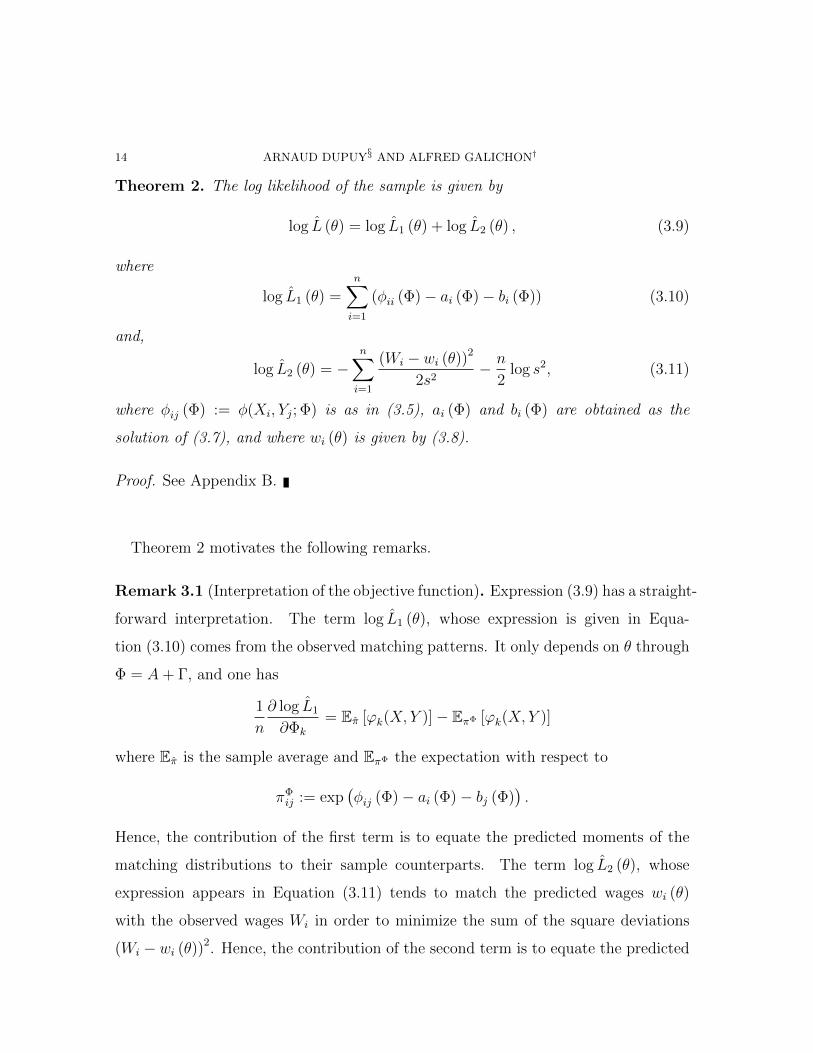
Theorem 2. The log likelihood of the sample is given by
log L (θ) = log L1 (θ) + log L2 (θ) , (3.9)
where
log L1 (θ) =n∑i=1
(φii (Φ)− ai (Φ)− bi (Φ)) (3.10)
and,
log L2 (θ) = −n∑i=1
(Wi − wi (θ))2
2s2− n
2log s2, (3.11)
where φij (Φ) := φ(Xi, Yj; Φ) is as in (3.5), ai (Φ) and bi (Φ) are obtained as the
solution of (3.7), and where wi (θ) is given by (3.8).
Proof. See Appendix B.
Theorem 2 motivates the following remarks.
Remark 3.1 (Interpretation of the objective function). Expression (3.9) has a straight-
forward interpretation. The term log L1 (θ), whose expression is given in Equa-
tion (3.10) comes from the observed matching patterns. It only depends on θ through
Φ = A+ Γ, and one has
1
n
∂ log L1
∂Φk
= Eπ [ϕk(X, Y )]− EπΦ [ϕk(X, Y )]
where Eπ is the sample average and EπΦ the expectation with respect to
πΦij := exp
(φij (Φ)− ai (Φ)− bj (Φ)
).
Hence, the contribution of the first term is to equate the predicted moments of the
matching distributions to their sample counterparts. The term log L2 (θ), whose
expression appears in Equation (3.11) tends to match the predicted wages wi (θ)
with the observed wages Wi in order to minimize the sum of the square deviations
(Wi − wi (θ))2. Hence, the contribution of the second term is to equate the predicted

ESTIMATION OF JOB AMENITIES AND LABOR PRODUCTIVITY 15
wages with their sample counterparts. Of course, s2 will determine the relative weight-
ing of those two terms in the joint optimization problem. If s2 is high, which means
wages are observed with a large amount of noise, then the first term becomes pre-
dominant in the maximization problem. In the limit s2 → +∞, the problem will boil
down to a two-stage problem, where the parameter Φ is estimated in the first stage,
and the rest of the parameters are estimated in the second stage by Non-Linear Least
Squares conditional on A+ Γ = Φ. In the MLE procedure, s2 is a parameter, and its
value is determined by the optimization procedure.
Remark 3.2 (Concentrated Likelihood). In most applications, the parameters of
primary interest are those governing workers’ deterministic values of amenities and
firms’ deterministic values of productivity, i.e. A and Γ respectively. The remaining
parameters (σ1, σ2, t, s2) are auxiliary, and the focus of attention is the concentrated
log-likelihood, which is given by
log l (A,Γ) := maxσ1,σ2,t,s2
log L (θ) = log L1 (Φ) + maxσ1,σ2,t,s2
log L2
(A,Γ, σ1, σ2, t, s
2).
where as usual, Φ = A + Γ. Denoting σ∗1, σ∗2, t∗ and s∗2 the optimal value of the
corresponding parameters given A and Γ, one gets
(σ∗1, σ∗2, t∗) = arg min
σ1,σ2,t
n∑i=1
(Wi − wi (θ))2 , (3.12)
which is the solution to a Nonlinear Least Squares problem which is readily imple-
mented in standard statistical packages, and s∗2 = n−1∑n
i=1 (Wi − wi (θ∗))2. The
partial derivative of the concentrated log likelihood with respect to Ak is given by
∂ log l (A,Γ)
∂Ak=∂ log L1 (Φ)
∂Φk
+∂ log L2 (A,Γ, σ∗1, σ
∗2, t∗, s∗2)
∂Ak
and a similar expression holds for ∂ log l/∂Γk. These formulas are proved in the
Appendix B.
Remark 3.3 (Extension to missing wages). In many applications, data will come
from surveys where typically non response to questions about earnings are frequently

16 ARNAUD DUPUY§ AND ALFRED GALICHON†
encountered. Our proposed estimation strategy extends to the case where, for some
matches, wages are randomly missing. The log likelihood expression presented in
Theorem 2 offers a very intuitive way of understanding how missing wages for some
observations will impact the estimation. To formalize ideas, let p be the probability
that for any arbitrary match the wage is missing. The sample is still representative of
the population of matches, but part of the sample consists of matches with observed
wages , i.e. (Xi, Yi,Wi)no
i=1, and the other part of matches with missing wages, i.e.
(Xi, Yi, .)ni=no+1 where no is the number of matches with observed wages and n is as
before the size of our sample of matches (we have re-ordered the observations such
that those matches with observed wages are indexed first). The log likelihood in this
situation is therefore
log L (θ) = log L1 (θ) + log L2 (θ) + no log p+ (n− no) log (1− p)
where log L1 (θ) is given as in Equation (3.10) and log L2 (θ) reads now as
log L2 (θ) = −no∑i=1
(Wi − wi (θ))2
2s2− no
2log s2 (3.13)
thus p = n0/n. As no tends to 0, and hence p tends to 0, the log likelihood function
tends to log L1 (θ). In contrast, when no tends to n, and hence p tends to 1, the
expression of log L2 (θ) in Equation (3.13) tends to that of log L2 (θ) in Equation (3.11)
such that the log likelihood function tends to Equation (3.9).
3.5. Gradient of the log-likelihood. Let Da and Db be the two n×K matrices of
respective terms ∂ai (Φ) /∂Φk and ∂bj (Φ) /∂Φk respectively. Let Π be the matrix of
terms πΦij = exp
(φij (Φ)− ai (Φ)− aj (Φ)
), and let Π be the same matrix where the
entries on the first row have been replaced by zeroes. Let E be the n×K matrix whose
terms Eik are such that E1k = 0 for all k, and Eik =∑n
j=1 πΦijϕk (xi, yj) for i ≥ 2 and
all k. Let F be the n×K matrix of terms such that Fjk =∑n
i=1 πΦjiϕk (xi, yj).
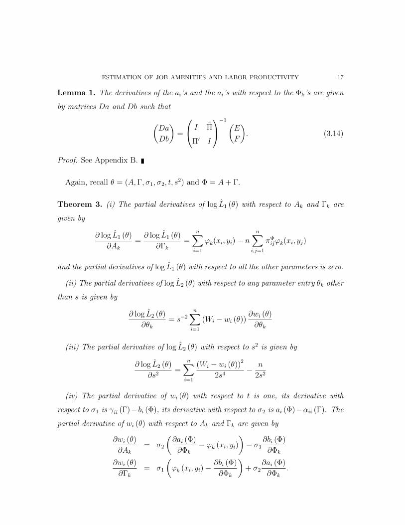
ESTIMATION OF JOB AMENITIES AND LABOR PRODUCTIVITY 17
Lemma 1. The derivatives of the ai’s and the ai’s with respect to the Φk’s are given
by matrices Da and Db such that
(Da
Db
)=
I Π
Π′ I
−1(E
F
). (3.14)
Proof. See Appendix B.
Again, recall θ = (A,Γ, σ1, σ2, t, s2) and Φ = A+ Γ.
Theorem 3. (i) The partial derivatives of log L1 (θ) with respect to Ak and Γk are
given by
∂ log L1 (θ)
∂Ak=∂ log L1 (θ)
∂Γk=
n∑i=1
ϕk(xi, yi)− nn∑
i,j=1
πΦijϕk(xi, yj)
and the partial derivatives of log L1 (θ) with respect to all the other parameters is zero.
(ii) The partial derivatives of log L2 (θ) with respect to any parameter entry θk other
than s is given by
∂ log L2 (θ)
∂θk= s−2
n∑i=1
(Wi − wi (θ))∂wi (θ)
∂θk
(iii) The partial derivative of log L2 (θ) with respect to s2 is given by
∂ log L2 (θ)
∂s2=
n∑i=1
(Wi − wi (θ))2
2s4− n
2s2
(iv) The partial derivative of wi (θ) with respect to t is one, its derivative with
respect to σ1 is γii (Γ)−bi (Φ), its derivative with respect to σ2 is ai (Φ)−αii (Γ). The
partial derivative of wi (θ) with respect to Ak and Γk are given by
∂wi (θ)
∂Ak= σ2
(∂ai (Φ)
∂Φk
− ϕk (xi, yi)
)− σ1
∂bi (Φ)
∂Φk
∂wi (θ)
∂Γk= σ1
(ϕk (xi, yi)−
∂bi (Φ)
∂Φk
)+ σ2
∂ai (Φ)
∂Φk
.
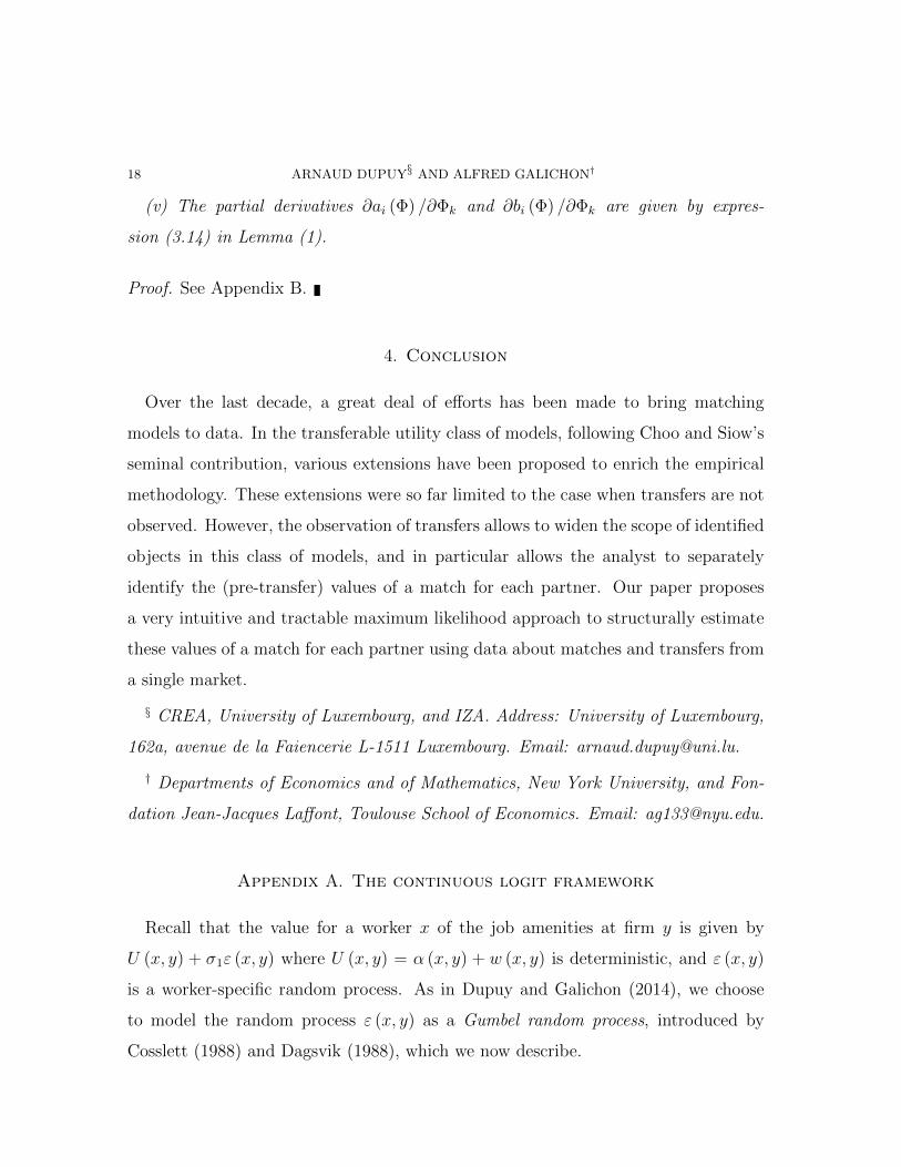
18 ARNAUD DUPUY§ AND ALFRED GALICHON†
(v) The partial derivatives ∂ai (Φ) /∂Φk and ∂bi (Φ) /∂Φk are given by expres-
sion (3.14) in Lemma (1).
Proof. See Appendix B.
4. Conclusion
Over the last decade, a great deal of efforts has been made to bring matching
models to data. In the transferable utility class of models, following Choo and Siow’s
seminal contribution, various extensions have been proposed to enrich the empirical
methodology. These extensions were so far limited to the case when transfers are not
observed. However, the observation of transfers allows to widen the scope of identified
objects in this class of models, and in particular allows the analyst to separately
identify the (pre-transfer) values of a match for each partner. Our paper proposes
a very intuitive and tractable maximum likelihood approach to structurally estimate
these values of a match for each partner using data about matches and transfers from
a single market.
§ CREA, University of Luxembourg, and IZA. Address: University of Luxembourg,
162a, avenue de la Faiencerie L-1511 Luxembourg. Email: [email protected].
† Departments of Economics and of Mathematics, New York University, and Fon-
dation Jean-Jacques Laffont, Toulouse School of Economics. Email: [email protected].
Appendix A. The continuous logit framework
Recall that the value for a worker x of the job amenities at firm y is given by
U (x, y) + σ1ε (x, y) where U (x, y) = α (x, y) + w (x, y) is deterministic, and ε (x, y)
is a worker-specific random process. As in Dupuy and Galichon (2014), we choose
to model the random process ε (x, y) as a Gumbel random process, introduced by
Cosslett (1988) and Dagsvik (1988), which we now describe.

ESTIMATION OF JOB AMENITIES AND LABOR PRODUCTIVITY 19
Assume that workers can only possibly have access to a countable random subset
of firms. We call this subset of known firms a worker’s “prospects”. Hence, a worker
can only choose to work for a firm within her prospects. Let k ∈ N index firms
in a worker’s prospects and {(yk, εk) , k ∈ N} be the points of a Poisson process on
Y × R with intensity dye−εdε. A worker of type x therefore chooses to work at firm
l of type yl = y in her prospects if and only if l is a solution of the worker’s utility
maximization program
U = maxy∈Y{U (x, y) + σ1ε (x, y)} = max
k∈N{U (x, yk) + σ1εk} ,
where U denotes the worker’s (random) indirect utility. The worker’s program induces
conditional density of choice probability of firm’s type given worker’s type, which is
expressed as follows:
Proposition A.1. The conditional density of probability of choosing a firm of type
y for a worker of type x is given by
π (y|x) =exp
(U(x,y)σ1
)∫Y exp
(U(x,y′)σ1
)dy′
while the expected indirect utility of worker x, denoted u (x) = E[U |x
], is expressed
as
u (x) = σ1 log
∫Y
exp
(U (x, y′)
σ1
)dy′.
This result was obtained by Cosslett (1988) and Dagsvik (1988). The intuition of
the result is that the c.d.f. of the random utility U conditional on X = x is given by
FU |X=x (z|x) = Pr(U ≤ z|X = x
), which is the probability that the process (yk, εk)
does not intersect the set {(y, e) : U (x, y) + σ1e > z}. Hence, the log probability of
the event U ≤ z is minus the integral of the intensity of the Poisson process over this

20 ARNAUD DUPUY§ AND ALFRED GALICHON†
set, that is
log Pr(U ≤ z|X = x
)= −
∫Y
∫R
1 {U (x, y) + σ1e > z} e−εdedy
= − exp
(−z + log
∫Y
exp
(U (x, y)
σ1
)dy
),
which is the c.d.f. of a Gumbel distribution with location parameter log∫Y exp (U(x, y)) dy,
and scale parameter σ1.
Appendix B. Proofs
Proof of Theorem 1. Part (i) is proved in Dupuy and Galichon (2014), Theorem 1,
and recalled below for completeness. It follows from Equations (2.1) and (2.2) that
π (y|x) = exp
(α (x, y)− u (x) + w (x, y)
σ1
), (B.1)
thus
σ1 log π (x, y) = α (x, y)− u (x) + σ1 log f (x) + w (x, y) (B.2)
and similarly on the other side of the market,
σ2 log π (x, y) = γ (x, y)− v (y) + σ2 log g (y)− w (x, y) . (B.3)
Adding Equation (B.2) to (B.3) yields
σ log (π (x, y)) = φ (x, y)− a (x)− b (y) (B.4)
where a (x) = u (x) − σ1 log f (x) − t and b (y) = v (y) − σ2 log g (y) + t, where t is
chosen so that a (x0) = 0, thus t = u (x0)− σ1 log f (x0). The potentials a and b that
appear in Equation (B.4) are such that π ∈M (f, g), i.e.∫Y exp (φ (x, y)− a (x)− b (y)) dy = f (x)∫X exp (φ (x, y)− a (x)− b (y)) dx = g (y) ,
.
Uniqueness of such (a, b) such that a (x0) = 0 is proved in Ruschendorf and Thomsen
(1993), Theorem 3.
ESTIMATION OF JOB AMENITIES AND LABOR PRODUCTIVITY 21
Let us now show (ii). Taking the logarithm of Equation (B.1) and rearranging
yields
u (x) = α (x, y) + w (x, y) + σ1 log f (x)− σ1 log π (x, y) (B.5)
A similar procedure using the expression for π (x|y) obtains,
v (y) = γ (x, y)− w (x, y) + σ2 log g (y)− σ2 log π (x, y) . (B.6)
Adding Equation (B.5) to (B.6) and using Equation (B.4) yields
u (x) + v (y) = σ1 log f (x) + σ2 log g (y) + a (x) + b (y) . (B.7)
By rearranging Equation (B.7) to obtain
u (x)− σ1 log f (x)− a (x) = σ2 log g (y) + b (y)− v (y)
one notes that since the right hand-side only depends on x and the left hand-side
only depends on y, both these terms must be equal to a constant, denoted t. Hence,
u (x) = a (x) + σ1 log f (x) + t, and (B.8)
v (y) = b (y) + σ2 log g (y)− t. (B.9)
Let us finally show (iii). Plugging Equation (B.8) into Equation (B.5) and rear-
ranging yields
w (x, y) = a (x)− α (x, y) + t+ σ1 log π (x, y) ,
which, using Equation (B.4) to substitute for log π (x, y), provides the following ex-
pression of the equilibrium wages as a function of α, γ, a, b and t,
w (x, y) =σ1
σ(γ (x, y)− b (y)) +
σ2
σ(a (x)− α (x, y)) + t. (B.10)
Proof of Theorem 2. Immediate given the discussion before the Theorem.
22 ARNAUD DUPUY§ AND ALFRED GALICHON†
Proof of Lemma 1. Recall that
(Da)ik :=∂ai (Φ)
∂Φk
and (Db)jk :=∂bj (Φ)
∂Φk
for 1 ≤ i ≤ n and 1 ≤ k ≤ K. Note that the system in Equation (3.2) is normalized
such that a1 (Φ) = 0, one has that ∂a1 (Φ) /∂Φk = 0 for all k. Differentiation yields
Da1k = 0
Da1k +n∑j=1
πΦijDbjk = Eik, i ∈ {2, ..., n}
n∑i=1
πΦijDaik +Dbjk = Fjk, j ∈ {1, ..., n} ,
where πΦij = exp
(φij (Φ)− ai (Φ)− aj (Φ)
). Recall that under the linear parameteri-
zation we have adopted in Section 3.3, ∂φij (Φ) /∂Φk = ϕk(xi, yj) and let
E1k = 0, Eik =n∑j=1
πΦijϕk(xi, yj) for i ≥ 2, and
Fjk =n∑i=1
πΦijϕk(xi, yj) for all j,
this system rewrites I Π
Π′ I
(DaDb
)=
(E
F
)(B.11)
where block Π is the n × n matrix of term πΦij so that πΦ
1j = 0 for all j ∈ {1, ..., n}
and πΦij = πΦ
ij for i ≥ 2 and all j ∈ {1, ..., n}, and block Π is the n×n matrix of term
πΦij. It is easily checked that the matrix on the left hand-side of (B.11) is invertible.
One therefore obtains Da and Db as
(Da
Db
)=
I Π
Π′ I
−1(E
F
).

ESTIMATION OF JOB AMENITIES AND LABOR PRODUCTIVITY 23
Proof of Theorem 3. The log-likelihood given in Equation (3.9) is made of two terms,
the first of which, log L1 (θ) only depends on θ through Φ, while the second one,
log L2 (θ) depends on all the parameters of the model. The differentiations yielding
points (i)-(v) are straightforward.
Proof of the statement in Remark 3.2. Recall θ = (A,Γ, σ1, σ2, t, s2). The maximum
likelihood problem can be written as
maxθ
log L (θ) = maxA,Γ
log l (A,Γ)
where log l (A,Γ) = maxσ1,σ2,t,s2 log L (θ) is the concentrated log-likelihood which can
be rewritten as
log l (A,Γ) = log L1 (θ) + maxσ1,σ2,t,s2
log L2 (θ) . (B.12)
where
maxσ1,σ2,t,s2
log L2 (θ) = −mins2
(n
2log s2 +
1
2s2minσ1,σ2,t
n∑i=1
(Wi − wi (θ))2
)(B.13)
The second minimization in Equation (B.13) is an Ordinary Least Squares problem
whose solution given A,Γ, denoted (σ∗1, σ∗2, t∗), is the vector of coefficients of the OLS
regression of W on (γ − b, a− α, 1). The value of s2, denoted s∗2, is given by
s∗2 =
∑ni=1 (Wi − wi (θ∗))2
n.
The envelope theorem yields an expression for the gradient of the concentrated
log-likelihood with respect to the concentrated parameters A and Γ, that is
∇A,Γ log l (A,Γ) = ∇A,Γ log L1 (θ∗) +∇A,Γ log L2 (θ∗) .
The elements of the first part of the gradient are given in Theorem 3 part (i) whereas
parts (ii), (iv) and (v) of Theorem 3 provide the building blocks for the elements of
the second part of the gradient.

24 ARNAUD DUPUY§ AND ALFRED GALICHON†
References
[1] Abowd, J., R.H. Creecy, and F. Kramarz (2002). “Computing Person and Firm Effects Us-
ing Linked Longitudinal Employer-Employee Data,” Technical Paper 2002-06, Longitudinal
Employer-Household Dynamics, Centre for Economic Studies, U.S. Census Bureau.
[2] Abowd, J., F. Kramarz, and D. Margolis (1999). “High Wage Workers and High Wage Firms”,
Econometrica, 67(2), pp. 251–333.
[3] Andrews, M.J., L. Gill, T. Schank, and R. Upward (2008). “High Wage Workers and Low
Wage Firms: Negative Assortative Matching or Limited Mobility Bias?” Journal of the Royal
Statistical Society, Series A, 171 (3), pp. 673-697.
[4] Andrews, M.J., L. Gill, T. Schank, and R. Upward (2012). “High Wage Workers Matched with
High Wage Firms: Clear Evidence of the Effects of Limited Mobility Bias,” Economics Letters,
117 (3), pp. 824-827.
[5] Becker, G. S. (1973). “A Theory of Marriage: Part I,” Journal of Political Economy, 81(4),
813–46.
[6] Becker, G. S. (1991). A Treatise on the Family. Harvard University Press.
[7] Berry, S, J. Levinsohn, and A. Pakes, (1995). “Automobile Prices in Market Equilibrium,”
Econometrica, vol. 63(4), pp. 841-90.
[8] Bojilov, R., and A. Galichon (2013). “Closed-form formulas for multivariate matching”. Mimeo.
[9] Brown, C. (1980). “Equalizing Differences in the Labor Market,” Quarterly Economics Jour-
nal ,” vol. 94 (1), pp. 113-134.
[10] Chiappori, P.-A., B. Salanie, and Y. Weiss (2015). “Assortative Matching on the Marriage
Market: A Structural Investigation,” working paper.
[11] Choo, E., and A. Siow (2006). “Who Marries Whom and Why,” Journal of Political Economy,
114(1), 175–201.
[12] Cosslett, S. (1988). “Extreme-value stochastic processes: A model of random utility maximiza-
tion for a continuous choice set,” Technical report, Ohio State University.
[13] Dagsvik, J. (1994). “Discrete and Continuous Choice, Max-Stable Processes, and Independence
from Irrelevant Attributes,” Econometrica 62, 1179–1205.
[14] Dupuy, A., and A. Galichon (2014). “Personality Traits and the Marriage Market,” the Journal
of Political Economy, vol. 122 (6), pp. 1271-1319.
[15] Ekeland, I., Heckman, J., and Nesheim, L. (2004). “Identification and estimation of Hedonic
Models”. Journal of Political Economy 112 (S1), pp. S60–S109.

ESTIMATION OF JOB AMENITIES AND LABOR PRODUCTIVITY 25
[16] Fox, J. (2010). “Identification in Matching Games,” Quantitative Economics 1, 203–254.
[17] Galichon, A., and B. Salanie (2015). “Cupid’s Invisible Hand: Social Surplus and Identification
in Matching Models,” working paper.
[18] Garen, J.E., (1988). “Compensating Wage Differentials and the Endogeneity of Job Riskiness,”
the Review of Economics and Statistics, vol. 70(1), pp. 9-16.
[19] Graham, B. (2011). “Econometric Methods for the Analysis of Assignment Problems in the
Presence of Complementarity and Social Spillovers,” in Handbook of Social Economics, ed. by
J. Benhabib, A. Bisin, and M. Jackson. Elsevier.
[20] Gretsky, N., J. Ostroy, and W. Zame (1992). “The nonatomic assignment model,” Economic
Theory, 2(1), 103–127.
[21] Gruetter, M. and R. Lalive (2009). “The Importance of Firms in Wage Determination,” Labour
Economics 16 (2), pp. 149-160.
[22] Heckman, J. J., Matzkin, R.L. and Nesheim, L. (2010). “Nonparametric Identi.cation and
Estimation of Nonadditive Hedonic Models”. Econometrica, 78 No. 5, pp. 1569-1591.
[23] Hwang, H.S., Reed, W.R. and Hubbard, C. (1992). “Compensating Wage Differentials and
Unobserved Productivity”. Journal of Political Economy, 100 No. 4, pp. 835.58.
[24] Lucas, Robert E B, (1977). “Hedonic Wage Equations and Psychic Wages in the Returns to
Schooling”, American Economic Review, vol. 67(4), pp. 549-58.
[25] Rosen, Sherwin, (1974). “Hedonic Prices and Implicit Markets: Product Differentiation in Pure
Competition,” Journal of Political Economy, vol. 82(1), pp. 34-55.
[26] Rosen, Sherwin, 1986. “The theory of equalizing differences,” Handbook of Labor Economics,
in: O. Ashenfelter & R. Layard (ed.), Handbook of Labor Economics, edition 1, volume 1,
chapter 12, pp. 641-692 Elsevier.
[27] Ruschendorf, L., and Thomsen, W. (1993). “Note on the Schrodinger Equation and I-
projections,” Statistics and Probability Letters 17, p. 369–375.
[28] Salanie, B. (2015). “Identification in Separable Matching with Observed Transfers,” Mimeo.
[29] Sattinger, M. (1979). “Differential Rents and the Distribution of Earnings,” Oxford Economic
Papers 31(1), pp. 60–71.
[30] Sattinger, M. (1993). “Assignment Models of the Distribution of Earnings,” Journal of Eco-
nomic Literature 31(2), pp. 831–80.

26 ARNAUD DUPUY§ AND ALFRED GALICHON†
[31] Shapley, L., and M. Shubik (1972). “The Assignment Game I: The Core,” International Journal
of Game Theory, 1, 111–130.Sattinger, M. (1978). “Comparative Advantage in Individuals”.
Review of Economics and Statistics, 60 No. 2, pp. 259–67.
[32] Thaler, R., and Rosen, S. (1976). “The Value of Saving a Life: Evidence from the Labor
Market.” In Household Production and Consumption, Nestor E. Terleckyj (ed.). New York:
NBER pp. 265–298.
[33] Torres, S. P. Portugal, J.T. Addison and P. Guimaraes, (2013). “The Sources of Wage Variation:
A Three-Way High-Dimensional Fixed Effects Regression Model”, IZA working paper No. 7276.
[34] Villani, C. (2003). Topics in Optimal Transportation. Lecture Notes in Mathematics, AMS.
[35] Villani, C. (2009). Optimal transport, old and new. Grundlehren der Mathematischen Wis-
senschaften, 338, Springer-Verlag, Berlin.
[36] Viscusi, W.K. and J. E. Aldy, (2003). “The Value of a Statistical Life: A Critical Review of
Market Estimates throughout the World,” Journal of Risk and Uncertainty, vol. 27(1), pp. 5-76.
[37] Woodcock, S.D. (2010). “Heterogeneity and Learning in Labor Markets,” The B.E. Journal of
Economic Analysis and Policy, Berkeley Electronic Press, 10 (1), pages 85.
Recommended