Discrete Exterior Calculus
Thesis by
Anil N. Hirani
In Partial Fulfillment of the Requirements
for the Degree of
Doctor of Philosophy
California Institute of Technology
Pasadena, California
2003
(Defended May 9, 2003)

ii
c© 2003
Anil N. Hirani
All Rights Reserved

iii
For
my parents Nirmal and Sati Hirani
my wife Bhavna and daughter Sankhya.

iv
Acknowledgements
I was lucky to have two advisors at Caltech – Jerry Marsden and Jim Arvo. It was Jim who convinced me to
come to Caltech. And on my first day here, he sent me to meet Jerry. I took Jerry’s CDS 140 and I think after
a few weeks asked him to be my advisor, which he kindly agreed to be. His geometric view of mathematics
and mechanics was totally new to me and very interesting. This, I then set out to learn.
This difficult but rewarding experience has been made easier by the help of many people who are at
Caltech or passed through Caltech during my years here. After Jerry Marsden and Jim Arvo as my advisors,
the other person who has taught me the most is Mathieu Desbrun. It has been my good luck to have him as
a guide and a collaborator. Amongst the faculty here, Al Barr has also been particularly kind and generous
with advice. I thank him for taking an interest in my work and in my academic well-being.
Amongst students current and former, special thanks to Antonio Hernandez for being such a great TA
in CDS courses, and spending so many extra hours, helping me understand so much stuff that was new to
me. Thanks also to the many Mathematics department TAs who had to suffer my incessant questioning in all
those maths courses. It wasn’t easy being an outsider in those courses, but they made the task easier. Thanks
to Sameer Jalnapurkar for giving me his fabulous notes on everything that is relevant; Dong-Eui Chang for
teaching me how to take fancy derivatives; Eitan Grinspun for his wit, politeness and for the chance to work
with him on discrete shells; Yiying Tong for collaboration on vector field decomposition; Mark Meyer for
doing so many things that were a precursor to the work in this thesis; Paul Penzes for the afternoon badminton
sessions; Adam Granicz and David Wei for being such nice and considerate current officemates and Eric Bax
for being such a peaceful and nice former officemate.
For the work in this thesis, I thank first of all the members of my Ph.D. committee – Jerrold E. Marsden
(chair), James Arvo, Mathieu Desbrun, Michael Ortiz and Peter Shcroder. Thanks to Jenny Harrison and
Alan Weinstein for taking an interest and pointing out several important issues to me; Alexander Givental for
reading parts of my thesis and giving me useful comments, and also for his exceptional teaching style – it
was a pleasure to sit in his classes when he spent some time at Caltech; Melvin Leok for collaboration and for
pointing out some important papers in the field; Arash Yavari for discussions and reading early versions of the
thesis. As I was finishing up I had the pleasure to work with Marco Castrillon and Antonio Fernandez who
were visiting Caltech around my defense time. They pointed out mistakes, and pointed out new directions,
even as this thesis was being written.

v
Thanks to my parents Nirmal and Sati, for instilling the respect and love for education and scholarship.
That upbringing made it so natural to leave the software industry, even when the internet craze was starting,
and return to academia. Thanks to my little daughter Sankhya, for making the evenings of last 4 years so
much fun. In her first 2 years of life she also taught me how to stay up all night! As for my wife Bhavna,
I cannot begin to thank her enough. I thank her for accepting this student life and agreeing to share the
uncertainty of academic life. I thank her for the moral support and love through the years. And for making
most of the figures that appear in this thesis. Thanks !
Finally, I want to thank Jerry Marsden again, for suggesting the problem of developing a discrete exterior
calculus – in what turned out to be September of my final year. It made these last few months very exciting.
The result is what this thesis is about.
This research was partially supported by NSF ITR grant ACI-0204932, and NSF Career Award CCR9876332.

vi
Abstract
The language of modern mechanics is calculus on manifolds, and exterior calculus is an important part of that.
It consists of objects like differential forms, general tensors and vector fields on manifolds, and operators that
act on these. While the smooth exterior calculus has a long history going back to Cartan, Lie, Grassmann,
Hodge, de Rham and many others, the need for a discrete calculus has been spurred on recently by the need
to do computations.
This thesis presents the beginnings of a theory ofdiscrete exterior calculus(DEC). This is motivated by
potential applications in computational methods for field theories (elasticity, fluids, electromagnetism) and in
areas of computer vision and computer graphics. One approach to approximating a smooth exterior calculus
is to consider the given mesh as approximating some smooth manifold at least locally, and then defining
the discrete operators by truncating the smooth ones. Another approach is to consider the discrete mesh
as the only given thing and developing an entire calculus using only discrete combinatorial and geometric
operations. The derivations may require that the objects on the discrete mesh, but not the mesh itself, are
interpolated. It is this latter route that we have taken and this leads to a discrete exterior calculus.
Our theory includes not only discrete equivalents of differential forms, but also discrete vector fields and
the operators acting on these objects. General tensors are not developed, though we suggest a possible way to
do that towards the end. The presence of forms and vector fields allows us to address the various interactions
between forms and vector fields which are important in applications. With a few exceptions, most previous
attempts at discrete exterior calculus have addressed only differential forms, or vector fields as proxies for
forms. We also show that the circumcentric dual of a simplicial complex plays a useful role in the metric
dependent part of this theory. The importance of dual complexes in this field has been well understood, but
with a few exceptions previous researchers have used barycentric duals.
The use of duals is reminiscent of the use of staggered meshes in computational mechanics. The appear-
ance of dual complexes leads to a proliferation of the operators in the discrete theory. For example there are
primal-primal, primal-dual etc. versions of many operators. This is of course unique to the discrete side.
In many examples we find that the formulas derived from our discrete exterior calculus are identitical to the
existing formulas in literature.
We define discrete differential forms in the usual way, as cochains on a simplicial complex. The discrete
vector fields are defined as vector valued 0-forms, and they live either on the primal, or on the dual vertices.

vii
We then define the operators that act on these objects, starting with discrete versions of the exterior derivative,
codifferential and Hodge star for operating on forms. A discrete wedge product is defined for combining
forms; discrete flat and sharp operators for going between vector fields and one forms; and discrete interior
product operator and Lie derivatives for combining forms and vector fields. The sharp and flat allow us to
define various vector calculus operators on simplicial meshes including a discrete Laplace-Beltrami operator.
Our development of the theory is formal in that we do not prove convergence to a smooth theory. We have
tried instead to build a discrete calculus that isself-consistent and parallels the smooth theory. The discrete
operator should be natural under pullbacks, when the smooth one is, important theorems like the discrete
Stokes’ theorem must be satisfied, and the operators should be local. We then use these operators to derive
explicit formulas for discrete differential operators in specific cases. These cases include 2-surfaces inR3
built with irregular triangles, regular rectangular and hexagonal meshes in the plane, and tetrahedralization
of domains inR3. At least in these simple but important examples we find that the formula derived from our
discrete exterior calculus is identitical to the existing formula in the literature.
Numerical methods similar to those based on a discrete exterior calculus have been used in many physi-
cal problems, for example, in areas like electromagnetism, fluid mechanics and elasticity. This is due to the
geometric content of many physical theories. In this thesis we give a glimpse into three fields of discrete,
geometric computations, which we have developed without an exterior calculus framework. These are ex-
amples of areas which are likely to benefit from a working DEC. They include discrete shells, a Hodge type
decomposition of discrete 3D vector fields on an irregular, simplicial mesh, and template matching.
One potential application of DEC is to variational problems. Such problems come equipped with a rich
exterior calculus structure and so on the discrete level, such structures will be enhanced by the availability of
a discrete exterior calculus. One of the objectives of this thesis is to fill this gap. An area for future work,
is the relationship between multisymplectic geometry and DEC. There are many constraints in numerical
algorithms that naturally involve differential forms, such as the divergence constraint for incompressibility of
fluids. Another example is in electromagnetism since differential forms are naturally the fields in that subject,
and some of Maxwell’s equations are expressed in terms of the divergence and curl operations on these fields.
Preserving, as in the mimetic differencing literature, such features directly on the discrete level is another one
of the goals, overlapping with our goals for variational problems.
In future work we want to make a cleaner separation of metric independent and metric dependent parts of
DEC. For example, the wedge product, pairing of forms and vector fields, interior product and Lie derivative,
should all be metric independent. Divergence should depend on the metric, only through the appearance of
volume form. The metric should play a role only in the definition of sharp and flat operators. In this thesis,
we don’t always make this distinction and sometimes use identities from smooth theory, where the metric
dependence cancels. It is not clear that the same cancellation happens on the discrete side. In these cases we
have also tried to give at least a partial development of a metric independent definition.
In this thesis we have tried to push a purely discrete point of view as far as possible. In fact, in various

viii
parts of the thesis we argue that this can only be pushed so far, and that interpolation is a useful device for
developing DEC. For example, we found that interpolation of functions and vector fields is a very convenient
device for understanding and deriving a discrete theory involving functions and vector fields. This naturally
leads to the next step, that of interpolation of higher degree forms, for example using Whitney map. This is
the methodology that is quite common in this field. In future work we intend to continue this interpolation
point of view, especially in the context of the sharp, Lie derivative and interior product operators. Some
preliminary ideas on this point of view are spread throughout the thesis.

ix
Contents
Acknowledgements iv
Abstract vi
1 Introduction 1
1.1 Results of This Thesis . . . . . . . . . . . . . . . . . . . . . . . . . . . . . . . . . . . . . . 2
1.2 The Objects in DEC . . . . . . . . . . . . . . . . . . . . . . . . . . . . . . . . . . . . . . . 3
1.3 History and Previous Work . . . . . . . . . . . . . . . . . . . . . . . . . . . . . . . . . . . 4
1.4 How This Thesis is Organized . . . . . . . . . . . . . . . . . . . . . . . . . . . . . . . . . 6
1.5 Increasing Role of Interpolation . . . . . . . . . . . . . . . . . . . . . . . . . . . . . . . . 6
2 Primal and Dual Complexes 8
2.1 Simplicial Complex . . . . . . . . . . . . . . . . . . . . . . . . . . . . . . . . . . . . . . . 8
2.2 Discretizing the Manifold . . . . . . . . . . . . . . . . . . . . . . . . . . . . . . . . . . . . 10
2.3 Oriented Primal Complex . . . . . . . . . . . . . . . . . . . . . . . . . . . . . . . . . . . . 11
2.4 Dual Complex . . . . . . . . . . . . . . . . . . . . . . . . . . . . . . . . . . . . . . . . . . 14
2.5 Oriented Dual Complex . . . . . . . . . . . . . . . . . . . . . . . . . . . . . . . . . . . . . 20
2.6 Circumcentric and Barycentric Duality . . . . . . . . . . . . . . . . . . . . . . . . . . . . . 22
2.7 Interpolation Functions . . . . . . . . . . . . . . . . . . . . . . . . . . . . . . . . . . . . . 24
2.8 Local and Global Embeddings . . . . . . . . . . . . . . . . . . . . . . . . . . . . . . . . . 25
2.9 Summary and Discussion . . . . . . . . . . . . . . . . . . . . . . . . . . . . . . . . . . . . 26
3 Discrete Forms and Exterior Derivative 28
3.1 Differential Forms and Discrete Forms . . . . . . . . . . . . . . . . . . . . . . . . . . . . . 28
3.2 Primal Chains and Cochains . . . . . . . . . . . . . . . . . . . . . . . . . . . . . . . . . . 29
3.3 Whitney and de Rham Maps . . . . . . . . . . . . . . . . . . . . . . . . . . . . . . . . . . 31
3.4 Dual Chains and Cochains . . . . . . . . . . . . . . . . . . . . . . . . . . . . . . . . . . . 33
3.5 Maps Between Complexes and Pullback of Forms . . . . . . . . . . . . . . . . . . . . . . . 34
3.6 Exterior Derivative . . . . . . . . . . . . . . . . . . . . . . . . . . . . . . . . . . . . . . . 35

x
3.7 Speculations on Convergence . . . . . . . . . . . . . . . . . . . . . . . . . . . . . . . . . . 38
3.8 Summary and Discussion . . . . . . . . . . . . . . . . . . . . . . . . . . . . . . . . . . . . 38
4 Hodge Star and Codifferential 40
4.1 Hodge Star . . . . . . . . . . . . . . . . . . . . . . . . . . . . . . . . . . . . . . . . . . . 40
4.2 Codifferential . . . . . . . . . . . . . . . . . . . . . . . . . . . . . . . . . . . . . . . . . . 42
4.3 Summary and Discussion . . . . . . . . . . . . . . . . . . . . . . . . . . . . . . . . . . . . 42
5 Forms and Vector Fields 44
5.1 Discrete Vector Fields . . . . . . . . . . . . . . . . . . . . . . . . . . . . . . . . . . . . . . 45
5.2 Smooth Flat and Sharp . . . . . . . . . . . . . . . . . . . . . . . . . . . . . . . . . . . . . 47
5.3 Proliferation of Discrete Flats and Sharps . . . . . . . . . . . . . . . . . . . . . . . . . . . 48
5.4 Discrete Flats . . . . . . . . . . . . . . . . . . . . . . . . . . . . . . . . . . . . . . . . . . 48
5.5 A Dual-Primal-Primal Flat . . . . . . . . . . . . . . . . . . . . . . . . . . . . . . . . . . . 49
5.6 Other Discrete Flats . . . . . . . . . . . . . . . . . . . . . . . . . . . . . . . . . . . . . . . 53
5.7 A Primal-Dual Sharp for Exact Forms . . . . . . . . . . . . . . . . . . . . . . . . . . . . . 54
5.8 A Primal-Primal Sharp . . . . . . . . . . . . . . . . . . . . . . . . . . . . . . . . . . . . . 56
5.9 Composing Sharps and Flats . . . . . . . . . . . . . . . . . . . . . . . . . . . . . . . . . . 56
5.10 Natural Pairing of Forms and Vector Fields . . . . . . . . . . . . . . . . . . . . . . . . . . 57
5.11 Summary and Discussion . . . . . . . . . . . . . . . . . . . . . . . . . . . . . . . . . . . . 58
6 Div, Grad, Curl and Laplace-Beltrami 59
6.1 Divergence . . . . . . . . . . . . . . . . . . . . . . . . . . . . . . . . . . . . . . . . . . . 60
6.2 Gradient . . . . . . . . . . . . . . . . . . . . . . . . . . . . . . . . . . . . . . . . . . . . . 64
6.3 Curl . . . . . . . . . . . . . . . . . . . . . . . . . . . . . . . . . . . . . . . . . . . . . . . 65
6.4 Laplace-Beltrami . . . . . . . . . . . . . . . . . . . . . . . . . . . . . . . . . . . . . . . . 68
6.5 Summary and Discussion . . . . . . . . . . . . . . . . . . . . . . . . . . . . . . . . . . . . 70
7 Wedge Product 71
7.1 Primal-Primal Wedge . . . . . . . . . . . . . . . . . . . . . . . . . . . . . . . . . . . . . . 71
7.2 Alternative Primal-Primal Wedge . . . . . . . . . . . . . . . . . . . . . . . . . . . . . . . . 74
7.3 Summary and Discussion . . . . . . . . . . . . . . . . . . . . . . . . . . . . . . . . . . . . 75
8 Interior Product and Lie Derivative 77
8.1 Separation of Forms and Vector Fields . . . . . . . . . . . . . . . . . . . . . . . . . . . . . 78
8.2 Algebraic Discrete Interior Product or Contraction . . . . . . . . . . . . . . . . . . . . . . . 79
8.3 Interior Product via Extrusion . . . . . . . . . . . . . . . . . . . . . . . . . . . . . . . . . 81
8.4 Algebraic Lie Derivative . . . . . . . . . . . . . . . . . . . . . . . . . . . . . . . . . . . . 83

xi
8.5 Lie Derivative From Flow-Out Formula . . . . . . . . . . . . . . . . . . . . . . . . . . . . 83
8.6 Summary and Discussion . . . . . . . . . . . . . . . . . . . . . . . . . . . . . . . . . . . . 85
9 Other Work 87
9.1 Template Matching . . . . . . . . . . . . . . . . . . . . . . . . . . . . . . . . . . . . . . . 87
9.2 Discrete Shells . . . . . . . . . . . . . . . . . . . . . . . . . . . . . . . . . . . . . . . . . 88
9.3 Discrete Multiscale Vector Field Decomposition . . . . . . . . . . . . . . . . . . . . . . . . 89
9.4 Regular Nonsimplicial Meshes . . . . . . . . . . . . . . . . . . . . . . . . . . . . . . . . . 92
9.5 General Discrete Tensors . . . . . . . . . . . . . . . . . . . . . . . . . . . . . . . . . . . . 95
9.6 Summary and Discussion . . . . . . . . . . . . . . . . . . . . . . . . . . . . . . . . . . . . 95

1
Chapter 1
Introduction
This thesis presents the beginnings of a theory ofdiscrete exterior calculus(DEC), motivated by potential
applications in computational methods for field theories (elasticity, fluids, electromagnetism), and in areas
of computer vision and computer graphics. This theory has a long history that we shall outline below in
Section 1.3, but we aim at a comprehensive, systematic, as well as useful, treatment. Many previous works,
as we shall review, are incomplete in terms of the objects and operators that they treat.
One approach to approximating a smooth exterior calculus is to consider the given mesh as approximating
some smooth manifold at least locally, and then defining the discrete operators by truncating the smooth ones.
Another approach is to consider the discrete mesh as the only given thing and developing an entire calculus
using only discrete combinatorial and geometric operations. The derivations of the operators may require that
the objects on the discrete mesh, but not the mesh itself, are interpolated. It is this latter route that we have
taken and this leads to a discrete exterior calculus. General views of the subject area of DEC are common
in the literature (see, for instance, Mattiussi [2000]), but they usually stress the process of discretizing a
continuous theory and the overall approach is tied to this goal. However we take the point of view that the
discrete theory can stand in its own right.
Applications to Variational Problems. One application is to variational problems. These arise naturally
in mechanics and optimal control. In addition many problems in computer vision, image processing and
computer graphics can also be posed naturally as variational problems. Some examples are template match-
ing, image restoration, image segmentation and computation of minimal distortion maps. See, for example,
Hirani et al. [2001]; Paragios [2002]; Gu [2002]; Desbrun et al. [2002]. Key ingredients for computations
involving variational principles, at least in mechanics, are variational integrators designed for the numerical
integration of mechanical systems, as in Lew et al. [2003]. These algorithms respect some of the key features
of the continuous theory, such as their (multi)symplectic nature and exact conservation laws. They do so
by discretizing the underlying variational principles of mechanics rather than discretizing the equations. It
is well known (see the reference just mentioned for some of the literature) that variational problems come
equipped with a rich exterior calculus structure and so on the discrete level, such structures will be enhanced

2
by the availability of a discrete exterior calculus. One of the objectives of this thesis is to fill this gap.
Structured Constraints. There are many constraints in numerical algorithms that naturally involve differ-
ential forms, such as the divergence constraint for incompressibility of fluids. Another example is in electro-
magnetism, since differential forms are naturally the fields in that subject, and some of Maxwell’s equations
are expressed in terms of the divergence and curl operations on these fields. See Hehl and Obukhov [2000] for
electromagnetism using differential forms. Preserving, as in the mimetic differencing literature, such features
directly on the discrete level is another one of the goals, overlapping with our goals for variational problems.
Methodology. We believe that one way to proceed with this program is to develop a calculus on discrete
manifolds which parallels the calculus on smooth manifolds. Indeed one advantage of developing a calculus
on discrete manifolds is pedagogical. By using concrete examples of discrete two- and three-dimensional
spaces one can explain most of discrete calculus at least formally. The machinery of Riemannian manifolds
and general manifold theory from the smooth case is, strictly speaking, not required in the discrete world.
The technical terms that will be used in the rest of this introduction will be defined in subsequent sections,
but they should be already familiar to someone who knows the usual exterior calculus on smooth manifolds.
Chapters 6 and 7 of Abraham et al. [1988] are a good standard reference.
Our development in this thesis is formal, in the sense that we choose appropriate geometric definitions
of the various objects and quantities involved. We do not prove that these definitions converge to the smooth
counterparts. The definitions are chosen so as to make some important theorems like the generalized Stokes’
theorem true by definition, to preserve naturality with respect to pullbacks, and to ensure that operators are
local. Often, an interpolation of objects is involved in reaching the discrete definition. In the cases where
previous results are available, we have checked that the operators we obtain match the ones obtained by other
means such as variational or other derivations. A proper study of convergence is clearly needed in the future
after we have had some numerical experience with DEC.
1.1 Results of This Thesis
Our development of discrete exterior calculus includes discrete differential forms as well as vector fields,
the Hodge star operator, the wedge product, the exterior derivative, as well as interior product and the Lie
derivative. Our theory can be thought of as calculus on simplicial complexes of arbitrary finite dimension.
We point out that the embedding of the complex can be local. We also hint at how it might generalize
formulas from finite-difference theory on regular meshes. The inclusion of discrete differential forms and
discrete vector fields allows us to address the various interactions between forms and vector fields which
are important in applications. With a few exceptions, such as Bossavit [2003], previous attempts at discrete
exterior calculus have addressed only differential forms, or have used vector fields as proxies for forms.
3
We use circumcentric duals of simplicial complexes in the metric parts of our theory. The importance
of dual complexes in this field has been well understood, but most previous researchers have used barycen-
tric duals. We show that circumcentric duals play a role in arriving at the metric dependent parts of a DEC
theory. This includes the sharp and flat operators for going between vector fields and forms, and the Hodge
star for operating on forms. The usefulness of circumcentric duality in these cases stems from the fact that
the property of being normal to boundary comes automatically with circumcentric duality. This makes the
expressions for fluxes very easy in terms of geometric objects like the dual cells. Indeed the importance of
circumcentric duals in this context has also been known in some communities such as the mimetic differenc-
ing. But that has usually been for flat two- or three-dimensional logically rectangular meshes and only scalar
and vector fields appear in that literature.
While most of the thesis is about discrete exterior calculus on a single discrete manifold we define discrete
pullback between two complexes. Multiple meshes are important in applications where the mesh is changing,
but the discrete pullback is important even for picking the right definition on a single complex in some cases.
This is because it provides the criterion of naturality for discrete operators, i.e., commuting with pullback,
which is important for a full calculus on manifold. This was pointed out to us very recently by Marco
Castrillon and Jerry Marsden.
We argue in this thesis, that interpolation of objects is important for developing DEC. We use interpolation
of 0-forms and vector fields viewed as vector valued 0-forms and argue that the proper development of sharp
operator, and consequently of gradient and curl, requires the interpolation of 1-forms. In the Chapter on
interior product and Lie derivative we argue that the interpolation of forms plays a crucial role in the derivation
of discrete version of these operators. But we do not carry out this program of interpolation of higher degree
forms in this thesis, leaving it for future work.
1.2 The Objects in DEC
To develop a discrete theory, one must define discrete differential forms along with vector fields and operators
involving these. Once discrete forms and vector fields are defined, a calculus can be developed by defining the
discrete exterior derivative (d), codifferential (δ) and Hodge star (∗) for operating on forms, discrete wedge
product (∧) for combining forms, discrete flat ([) and sharp (]) operators for going between vector fields and
one forms and discrete interior product operator (iX ) for combining forms and vector fields. Once these are
done one can then define other useful operators. For example, a discrete Lie derivative (£X ) can bedefined
by requiring that the Cartan magic (or homotopy) formula hold. A discrete divergence in any dimension and
curl in R3 can also be defined. A discrete Laplace-Beltrami operator (∆) can be defined using the usual
definition ofdδ + δd. When applied to functions this is the same as the discrete Laplace-Beltrami operator
(∇2) which is the defined asdiv grad. We define all these objects and operators in this thesis. In some cases
we define the operators in multiple ways.

4
The discrete manifolds we work with are manifold-like oriented simplicial complexes (however we also
show how DEC generalizes some finite-difference formulas on regular non-simplicial meshes). We will recall
the standard formal definitions in Section 2.1 but familiar examples of simplicial complexes are meshes of
triangles embedded inR3 and meshes made up of tetrahedra occupying a portion ofR3. We will assume
that the angles and lengths on such discrete manifolds are computed in the embedding spaceRN using the
standard metric of that space. In other words in this thesis we do not address the issue of how to discretize
a given smooth Riemannian manifold and how to embed it inRN since there may be many ways to do this.
For example,SO(3) can be embedded inR9 with a constraint or inR4 using quaternions. For the purposes
of exterior calculus, only local metric information is required, and we will comment in Section 2.8 on how to
address the issue of embedding in a local fashion. We emphasize that we donot need a global embedding of
the discretized manifold, since the operators of DEC are local, and intrinsic. For simplicity of presentation
we don’t always stress this point and often write as if a global embedding has been given.
1.3 History and Previous Work
The use of simplicial chains and cochains (defined in Chapter 3) as the basic building blocks for a discrete
exterior calculus has appeared in several papers. See, for instance, Sen et al. [2000], Adams [1996], Bossavit
[2002b] and references therein. These authors view forms as linearly interpolated versions of smooth differ-
ential forms, a viewpoint originating from Whitney [1957], who introduced the Whitney and de Rham maps
that establish an isomorphism between simplicial cochains and Lipschitz differential forms. Similar ideas
on non-simplicial meshes and from a finite-difference point of view are referred to in the papers of Hyman,
Shashkov and their collaborators. See for instance Hyman and Shashkov [1997a] and the references therein.
These papers however use vector fields as proxies for forms.
Discrete forms for logically rectangular meshes are defined in Chard and Shapiro [2000]. They however
define only thed operator from exterior calculus. However it is interesting to see that the implementation
of even a subset of DEC-like ideas can be interesting for computational mechanics. Cochains are discrete
objects that can be paired with chains of oriented simplices or their geometric duals by the bilinear pairing of
evaluation. Intuitively, the natural pairing of evaluation can be thought of as integration of the discrete form
over the chain.
There is much interest in a discrete exterior calculus in the computational electromagnetics community, as
represented by Bossavit [2001, 2002b,a, 2003], Gross and Kotiuga [2001], Hiptmair [1999, 2001a,b, 2002b],
Mattiussi [1997, 2000], Teixeira [2001] and Tonti [2002]. This is the community that seems to have gone the
furthest in terms of incorporating DEC-like ideas into their computational methods. This is perhaps because
Maxwell’s equations can be written purely in terms of differential forms. With the exception of some recent
work of Bossavit on interior products (Bossavit [2003]) the computational electromagnetism community has
used either a forms only theory or with vector fields as proxies for forms.

5
Many of the authors cited above, for example, Bossavit [2002b], Sen et al. [2000], Hiptmair [2002b,a],
also introduce the notions of dual complexes in order to introduce the Hodge star operator. With the exception
of Hiptmair, they mostly use barycentric duals. This works fine if one develops a theory of discrete forms
and does not introduce discrete vector fields. We show later that to introduce discrete vector fields into the
theory the notion of circumcentric duals seems to be convenient.
Other authors, such as Moritz [2000]; Moritz and Schwalm [2001]; Schwalm et al. [1999, 2001] have
incorporated vector fields into the cochain based approach to exterior calculus by identifying vector fields
with cochains, and having them supported on the same mesh. This may make it harder to encode physically
relevant phenomena such as fluxes across boundaries that are important in some applications.
Another approach to a discrete exterior calculus is in Dezin [1995]. He defines a one-dimensional dis-
cretization of the real line in much the same way we would. However to generalize to higher dimensions he
introduces a tensor product of this space. This results in logically rectangular meshes. Our calculus however
is over simplicial meshes. A further difference is that like other authors in this field, Dezin [1995] does not
introduce vector fields into his theory. A related effort for three-dimensional domains with logically rectan-
gular meshes is that of Mansfield and Hydon [2001], who established a variational complex for difference
equations by constructing a discrete homotopy operator. In Harrison [1993, 1999] one finds the development
of a discrete calculus by extending the permitted domains of integration to include nonsmooth and fractal
spaces. These papers not only develop a part of discrete calculus but also discuss convergence issues. Be-
sides the exterior derivative, a Hodge star and Laplace-Beltrami are also defined in Harrison [1999] for very
general spaces.
In computer graphics Meyer et al. [2002] define, for simplicial meshes, discrete differential geometry
operators and vector calculus operators like Laplace-Beltrami. Recently Gu [2002] has done some very
interesting work in applying homology and cohomology theory for some applications in graphics, such as,
finding global conformal maps for arbitrary genus surfaces. However, they do not develop a discrete exterior
calculus. For instance, their wedge product is the standard one (cross product) inR3.
Mimetic discretization (Hyman and Shashkov [1997a]) is a successful development of finite-difference
and finite-volume type methods that satisfy various theorems like Stokes’ theorem. It has been applied to
a variety of physical problems. Once again, it is a theory that has been developed for forms only or vector
fields as proxies for forms. Also, most of those methods seem to be for flat meshes. Moreover, we conjecture
that a generalization of DEC for non-simplicial meshes will bring DEC and mimetic discretization closer,
except that in addition one will have a theory of forms and fields with all the attendant operators, and have it
for non-flat meshes as well. With the current version of DEC we have already made a start towards this, for
simplicial meshes.
6
1.4 How This Thesis is Organized
In chapters 2-8 the preamble of each chapter, i.e. the part before the numbered sections of the chapter begin,
summarizes what the chapter is about, the main new results in the chapter, the context in which the chapter
fits into DEC. This is typically the content of the first or first few paragraph of each chapter’s preamble.
The second part of each preamble is generally a summary of what remains to be done and what is not well-
understood etc. Chapter 9 is about other work and speculative work. The former consists of applications
that we have done which would benefit from a DEC like framework for their future development. The latter,
consists of some preliminary ideas about lattices and regular nonsimplicial complexes and general discrete
tensors. In some chapters the last section is a summary and discussion section. Due to this organization of the
thesis, we have not included a conclusions Chapter. The preambles and summary sections of the following
chapters, and the next section of this Chapter can be read instead, to understand the scope, limitations and
conclusions of this thesis.
1.5 Increasing Role of Interpolation
In this section we document our changing viewpoint about interpolation. Interpolation has been playing an
increasing role as we have gained more experience with DEC. When we started work on DEC, we held the
viewpoint of treating forms strictly as cochains, not only in the definition of forms, but also in the definition
of operators on forms. That is, we wanted to define all the operators of exterior calculus as cochains, using
only the values of the operands on chains. This was in contrast with another popular approach, such as that of
Sen et al. [2000] and others, in which forms are interpolated using Whitney maps, and operators defined on
the interpolated forms. An early consequence of our strictly discrete approach, was, for example the lack of
associativity of wedge product, except for closed forms (Remark 7.1.4). But the straightforward interpolation
approach mentioned above also suffers from not having an associative wedge product Sen et al. [2000]. Thus
while this lack of associativity has consequences for the theory, we pressed ahead.
But slowly there were other signs that a strict discrete approach was inconvenient. For example, we had
found a formula for a discrete flat operator without interpolating vector fields or forms. But it was found by
guesswork, by requiring a discrete divergence theorem to be true. Later, we realized that if we interpolated
vector fields, as interpolated vector valued 0-forms, we were able to give a derivation for the formula we had
found,andfind other types of discrete flats that we had missed. Thus the interpolation point of view seemed
to be good not just for explaining existing formulas, but for finding new ones. Similarly, we found that for
defining a discrete gradient, the point of view of interpolation of 0-forms inside simplices, was a useful one.
Similar advantages held for other vector calculus operators as we saw in our vector field decomposition work
in Tong et al. [2003].
Naturally, the question was, why stop at 0-forms ? Why not interpolate higher degree forms as well ? This

7
was obvious when we considered sharp operator on 1-forms and interior product and Lie derivative. With the
strictly discrete point of view, one can get quite far, but not all the way, it seems. We argue in this thesis that
the development of a sharp, gradient, interior product and Lie derivative requires the interpolation of one and
higher degree forms. The full development of this interpolation point of view is for future work.
One track for our future work, is the usual Whitney interpolation idea, studied by so many other authors.
This is to interpolate forms using Whitney forms and then use the smooth operators. But we intend to use it
to define operators like Lie derivative, that others have not explored. Another track we intend to explore, is if
we can build higher degree forms, defined everywhere on the complex, from 1-forms. This is along the same
lines as our preliminary suggestion to build general tensors by using tensor products of 1-forms as mentioned
in Section 9.5.
Even while knowing the limitations of a purely discrete approach, in this thesis, we try to push the purely
discrete point of view as far as possible. This is done, in part to expose the parts of DEC where interpolation
is clearly the way to go. We have tried to include the basic ideas about interpolation at various places in the
thesis, in preparation for our future work along this direction. This approach can be called a finite element
approach to DEC. Here, the discretization of forms via the de Rham map of Section 3.3 takes a back seat
and the interpolation of forms via Whitney maps or other means becomes more prominent. The operators are
defined on interpolated forms, by using the smooth definitions where possible.
Various interpolation schemes can then be studied, including higher order ones. Building a higher order
DEC requires that one find a closed way to construct higher degree forms from discrete 1-forms that are
quadratic or higher order accurate. In any case, even in the lowest order case, with this interpolation, or
finite element approach, there is no longer any need to define operators using metric information when the
smooth operators do not depend on the metric. This simplifies the presentation of DEC which can then be
organized into the metric-independent part like exterior derivative, wedge, interior product and Lie derivative,
and the metric dependent part like sharp and flat. It is quite possible, as happened in the case of flat, that the
interpolation based definition of some operators will eventually result in a purely discrete definition. This is
because the operators are all local and many involve derivatives. The identities from smooth theory that we
were forced to adopt as definitions in some cases, then become theorems in such a discrete theory.
The detailed exploration of such an interpolation based DEC, in which interpolation of higher degree
forms, and not just of 0-forms, plays a prominent role, is left for our immediate future work.

8
Chapter 2
Primal and Dual Complexes
Results: In our formulation of discrete exterior calculus,K, an oriented manifold-like simplicial complex
(defined below) discretizes a portion ofM , the triangulable Riemanniann-manifold of interest. The starting
point for our calculusis the given complexK. In this chapter we give basic definitions related to simpli-
cial complexes and their dual cell complexes and orientations of these. We have found a simple geometric
interpretation of orientation of duals which we give in this chapter. In contrast, in algebraic topology the
definition of dual orientation usually requires some knowledge of homology and relative homology theory.
The requirement of orientability may not be a problem in practice. This is because the operators in DEC are
local and any point of ann-manifold is in an open set that is homeomorphic to an open set inRn or in a half
space, in the case of boundary points.
Shortcomings: A complete treatment of DEC should discuss how wellK approximatesM , and indeed
howK is obtained fromM in the first place. It should also include a discussion of how well the discrete
operators approximate the smooth counterparts. But for this one needs to define a topology on the discrete side
so that continuity and convergence can be discussed. This discussion, of discretization and approximation
quality, is something we do not do in this thesis, although it is an important topic for future work. Nevertheless
in Section 2.2 we discuss the idea of discretization at least roughly.
2.1 Simplicial Complex
We now recall some basic definitions of simplices and simplicial complexes. For more details see Munkres
[1984] and Hatcher [2002]. Letv0, . . . , vp be a set of geometrically independent points inRN , i.e., the
vectorsv1 − v0, . . . , vp − v0 or equivalentlyv1 − v0, v2 − v1, . . . , vp − vp−1 are linearly independent.
Definition 2.1.1. A p-simplex σp is the convex hull ofp + 1 geometrically independent pointsv0, . . . , vp.
That is
σp =x ∈ RN
∣∣ x =∑p
i=0µivi whereµi ≥ 0 and
∑n
i=0µi = 1
.

9
We’ll write σp = v0 . . . vp. The pointsv0, . . . , vp are inRN and are called theverticesof the simplex, and the
numberp is called thedimensionof the simplex. Any simplex spanned by a (proper) subset ofv0, . . . , vp
is called a(proper) faceof σp ; their union is called theboundary of σp and denotedBd(σp). Theinterior
of σp is Int(σp) = σp\Bd(σp) and is also called anopen simplex. If σq is a proper face ofσp, then we
write σq ≺ σp. Sometimes we will writeσp asσ when the dimension is understood. By|σp| we will mean
thep-volume of σp in RN . Forp = 0 this is defined to be 1. The smallest affine subspace ofRN containing
σ is called theplane of σ and denotedP(σ). This can be obtained for example, by letting the coefficientsµ
above be negative. ♦
Definition 2.1.2. A simplicial complexK in RN is a collection of simplices inRN such that
(1) Every face of a simplex ofK is inK.
(2) The intersection of any two simplices ofK is either a face of each of them, or it is empty.
The dimensionn of the largest dimensional simplex inK will be called the dimension ofK. The union
of simplices ofK is a subset ofRN and will be called theunderlying spaceof K or the polytope of
K and denoted|K|. We will be only concerned withfinite simplicial complexes (a complex with a finite
number of simplices). In acell complex(also known asCW complex) open simplices are replaced bycells,
which are objects homeomorphic to open balls. See page 5 of Hatcher [2002] for another way to define cell
complexes. ♦
Remark 2.1.3. Topology on underlying space: For a finite complex (the only kind we will consider in
this work) the topology on|K| will be the natural one (subspace topology) induced fromRN . For a simplex
σp of dimensionp ≥ 1 the meaning ofInt(σp) andBd(σp) coincides with the usual topological meanings
of interior and boundary in the topology of|K|. However forp = 0, i.e., for pointsσ0, Int(σ0) = σ0 and
Bd(σ0) = ∅, since a point has no proper faces (see Def. 2.1.1). However in the topology of|K| a point has
empty topological interior and is its own topological boundary. This special status of a 0-simplex is actually
useful in defining duals as we will do in Def. 2.4.5. Another thing to keep in mind is that theInt(σp) for any
dimensionp is called anopensimplex even though (for example)Int(σ1) in a dimension 2 complex is not an
open set in the subspace topology. Forp = n the open simplexInt(σp) is indeed an open set. ♦
Definition 2.1.4. A flat (or linear) simplicial complexK of dimensionn in RN is one of which all simplices
are in the same affinen-subspace ofRN . This coincides with our usual intuition of a flat 2-surface embedded
in R3. ♦
Definition 2.1.5. A simplicial triangulation of the polytope|K| is any simplicial complexL such that the
union of the simplices ofL (i.e., polytope|L|) is the polytope|K|. ♦
Definition 2.1.6. If L is a sub-collection ofK that contains all faces of its elements, thenL is a simplicial
complex in its own right, and it is called asubcomplexof K. One subcomplex ofK is the collection of all

10
simplices ofK of dimension at mostp, which is called thep-skeletonof K and is denotedK(p). Theclosed
star (or one-ring) of a simplexs in K is denotedSt s and is the union of all simplices ofK havings as a
face. Twop-simplices will be calledadjacentof they share a(p− 1)-face. ♦
2.2 Discretizing the Manifold
Let M be a smooth triangulable Riemanniann-manifold and define an abstract simplicial complex onM .
See pages 15–19 of Munkres [1984] for the definition of and information on abstract simplicial complexes,
but for our purpose it is enough to think of it as simplices “glued” to or “drawn on”M in such way that they
form a “curved” simplicial complex. It is a cell complex in which the cells are simplices on the manifold.
Let K be a concrete geometric simplicial complex that is isomorphic to a part of the complex onM .
It may be convenient to embedK in RN whereN ≥ n. For example, this is often done in computational
mechanics and graphics when a surface is approximated by a triangle mesh embedded inR3. We stress that
the idea of discretization isnot to put charts on the manifold and then triangulate the codomain of the chart
into a simplicial complex. If we did this, then the idea of discrete approximation would be lost, because we
would have to store the analytical information about the chart exactly. Sometimes this is not even possible. An
example of this situation is when the smooth manifold can only be sampled by some physical measurement
such as when the shape of an object is acquired by scanning. So the simplices ofK approximate a portion of
M for which we may only know a set of points. These then become the vertices ofK. Nevertheless we will
define the following map.
Definition 2.2.1. LetσpM be an abstract simplex onM and a simplexσp
K be a simplex inK that approximates
it. In order to transfer information (like forms and vector fields) fromM to K we will need the exact or
approximate map between the two. We will call such a mapπσ : σpM → σp
K a pasting mapand assume it is
a smooth map. ♦
Remark 2.2.2. Pasting map as a formal device:We have mentioned above that in applications we may
not even knowM exactly. Thus the pasting maps will not be known in these cases. Even if they were,
storing the pasting maps would defeat the idea of discretization. But there is no harm in using them during
discretization. In general they are a formal device allowing one to talk about the transfer of information from
M to K. In practice they may be a procedural scheme or a measurement device allowing one to discretize
smooth information onM . If M is a domain inRN , then it may even be an identity map. ♦
Approximating a portion ofM by K means that the metric onK induced fromRN approximates the
metric onM in the portion being approximated. The embedding of the simplicial complex into an ambient
space is a computational convenience. For the purposes of the theory, it is only necessary to specify the
connectivity of the mesh in the form of an abstract simplicial complex, along with a local metric on the space

11
of vertices. This is addressed in Section 2.8. Discretization of forms via de Rham map and interpolation of
forms via Whitney maps is addressed in Section 3.3.
2.3 Oriented Primal Complex
For DEC we need a notion of orientation for the simplices and for simplicial complexes. We start with
simplices.
Definition 2.3.1. Define two orderings of the vertices of a simplexσp to be equivalent if they differ from
one another by an even permutation. Ifp > 0, then the orderings fall into two equivalence classes. Each
of these classes is called anorientation of σp. An oriented simplex (also writtenσp) is a simplex together
with an orientation. Ifv0, . . . , vp are the vertices ofσp, then we’ll use[v0, . . . , vp] for the oriented simplex
σp with the equivalence class of the ordering(v0, . . . , vp). A 0-simplex has only one possible ordering so has
no orientation (although it can have aninducedorientation defined below). ♦
Definition 2.3.2. Given a simplexσp with verticesv0, . . . , vp, the ordered collection of vectors(v1 −
v0, v2 − v0, . . . , vp − v0), which is a basis for the planeP(σ), will be called acorner basis atv0 of the
simplex. The ordered collection(v1− v0, v2− v1, . . . , vp− vp−1), which is also another basis, will be called
polyline basis fromv0 of the simplex. ♦
Remark 2.3.3. Simplex orientation using a basis:A simplexσ is a closed connected subset of its plane
P(σ) and of the same dimension as the plane. The planeP(σ) being an affine subspace ofRN is oriented in
the usual sense of orientation by an ordered basis or equivalently a volume form. In particular the ordered
corner basis and the polyline basis of the simplex orient the plane and hence the simplex itself. These notions
of orientation via corner and polyline basis coincide with the orientation via permutations defined above. This
means that the partition of the set of simplices into two orientation classes is the same in each case. See, for
example, Lemma 5a on page 360 of Whitney [1957]. Thus orienting a simplex is equivalent to orienting its
plane. From now we will use the word orientation to mean any of these equivalent notions of corner, polyline
or permutation based orientation. ♦
Example 2.3.4. Oriented simplices: Consider 3 non-collinear pointsv0, v1 and v2 in R2 labeling the
vertices of a triangle in a counterclockwise fashion. Then these three points individually are examples of 0-
simplices (hence these have no orientation). Examples of oriented 1-simplices are the oriented line segments
[v0, v1], [v1, v2] and [v0, v2]. By writing the vertices in that order we have given orientations to these 1-
simplices, i.e.,[v0, v1] is oriented fromv0 to v1. The triangle[v0, v1, v2] is a counterclockwise oriented
2-simplex.
Consider a simplexσp with verticesv0, . . . , vp with p ≥ 1. By deleting one vertex at a time from
this set we can enumerate the simplices that have dimension(p − 1) and are faces ofσp. There arep + 1

12
such faces and facei is spanned byv0, . . . , vi, . . . , vp for i = 0, . . . , p. The hat means omit that vertex.
An oriented simplexσp induces an orientation on each of these faces. The notion of induced orientation is
related to the boundary operator to be defined in Chapter 3 in Def. 3.6.1. But induced orientation can be
defined independently as follows.
Definition 2.3.5. Let σp = [v0, . . . , vp] be an oriented simplex, withp ≥ 1. This orientation ofσ gives each
of the(p − 1)-dimensional faces aninduced orientation. Forp > 1, if i is even the induced orientation of
the facev0 . . . vi . . . vp is the same as the orientation of the oriented simplex[v0, . . . , vi, . . . , vp]. Otherwise
it is the opposite one. ♦
Example 2.3.6. Induced orientation: Given the counterclockwise oriented triangleσ = [v0, v1, v2] its
unoriented 1-faces arev1v2, v0v2 andv0v1. The induced orientation onv1v2 is the same as the orientation of
[v1, v2]. The induced orientation onv0v2 is the opposite of the orientation of[v0, v1] and the induced orien-
tation onv0v1 is the same as the orientation of[v0, v1]. As another example consider an oriented tetrahedron
[v0, v1, v2, v3] with v0 at the top andv1, v2, v3 labeling the bottom triangle in counterclockwise fashion when
looked from outside. This has the same orientation class as the ordered collection of 3 vectors emanating from
v0 and pointing to the 3 verticesv1, v2 andv3 in order, i.e., the corner basis atv0. This corresponds to a right-
hand rule orientation for the plane of the tetrahedron, i.e., forR3. By the definition of induced orientation the
triangular faces of the tetrahedron get oriented counterclockwise when looking from outside.
Remark 2.3.7. Comparing orientations: Consider two oriented simplicesσ andτ embedded inRN .
If their dimensions differ, then their orientations cannot be compared. So assume that they have the same
dimensionp and so1 ≤ p ≤ n (0-simplices have no orientation). Then their orientations can be compared in
the following cases:
1. Their planes coincide, i.e.,P(σ) = P(τ)
2. They share a face of dimensionp− 1
In case 1 the two simplicesσ andτ will have the same orientation iff their corner or polyline basis orients
their plane the same way. In case 2 the two will have the same orientation if the induced orientation of the
sharedp− 1 face induced by theσ is opposite to that induced byτ . Fig. 2.1 clarifies this remark. ♦
Definition 2.3.8. Let σp andτp, with 1 ≤ p ≤ n, be two simplices whose orientations can be compared, that
is, they fall into one of the two cases of Rem. 2.3.7. If their orientations are in the same class we will say that
the two simplices have arelative orientation of +1 otherwise−1. We will write this assgn(σp, τp) = +1
or−1 respectively. ♦
The notion of a simplicial complex defined in this section is too general for our purpose. For example, in
R2 a triangle with a line segment sticking out of one vertex is a simplicial complex. While such things may

13
(a) (b)
Figure 2.1: Situations where orientations of simplices can be compared: (a) All the triangles are inR3 butsince their plane is identical (shown in the figure) the orientations can be compared using any of their cornerbasis or polyline basis. See Rem. 2.3.3 and 2.3.7 ; (b) Two triangles inR3 not in the same plane. Butsince they share an edge their orientations can be compared. Orienting them so that they induce oppositeorientations on the shared edge gives the two triangles identical orientations.
be useful say, in modeling domains connected by wires in electromagnetism, in this thesis we exclude such
cases by using the definition to be given below. Another type of complex to be excluded is, for example, two
triangles touching only at a common vertex. Excluding such complexes is in line with this being a theory
of exterior calculus. For example, in smooth exterior calculus the starting point is the notion of a smooth
manifold. The examples just mentioned can be considered to be discretizations of smooth spaces that are
not manifolds (not even manifolds with boundary) since they are not locally homeomorphic toRn or to half
space. This is captured in the following definition.
Definition 2.3.9. A simplicial complexK of dimensionn is called amanifold-like simplicial complex
if the underlying space|K| is aC0 manifold (possibly with boundary). In such a complex all simplices
of dimensionk with 0 ≤ k ≤ n − 1 must be a face of some simplex of dimensionn in the complex.
Also, by definition ofC0 manifolds each point on|K| will have a neighborhood homeomorphic toRn or
n-dimensional half-space. See pages 143 and 478 of Abraham et al. [1988] for definitions of manifolds and
manifolds with boundary. ♦
From now on we will work only with manifold-like simplicial complexes. Allowing only such complexes
has the added advantage that we can now define orientability for simplicial complexes. In algebraic topology
the definition of an orientable simplicial complex requires some technical machinery (such as homology
n-manifolds and homology groups). In the following definition we can bypass such machinery.
Definition 2.3.10. A manifold-like simplicial complexK of dimensionn is called anoriented manifold-
like simplicial complex if adjacentn-simplices (i.e., those that share a common(n− 1)-face) have the same
orientation (orient the shared(n − 1)-face oppositely) and simplices of dimensionsn − 1 and lower are
oriented individually. From now on the nameprimal mesh will be used to mean a manifold-like oriented

14
simplicial complex. ♦
2.4 Dual Complex
An important ingredient of DEC is the dual complex (defined below) of a manifold-like simplicial complex.
The dual complex will usually not be a simplicial complex. However if the primal mesh satisfies some
conditions, then the dualcanbe built from a simplicial refinement of the primal mesh. The notion of duality
we use is circumcentric (or Voronoi) duality. The other popular choice in this subject is barycentric duality
and we compare the two types in Section 2.6.
Remark 2.4.1. Metric-dependence and duality: The metric-dependent and metric-independent parts of
DEC can be developed separately. Operators, that in the smooth theory do not use metric information, should
have that property in the discrete theory as well. For example, the exterior derivative, wedge product, natural
pairing of forms and vector fields, interior product and Lie derivative are all example of such operators. On
the other hand Hodge star, sharp and flat depend on the metric. Divergence is an operator in which metric
enters only through its dependence on the volume form of the metric. Dual meshes seem to be required only
in the metric-dependent parts of DEC. However, in applications these might be all mixed up and thus one is
forced to invent versions of metric-independent operators for the dual mesh as well. An example is say, the
Lagrangian for harmonic maps,d f ∧ ∗d f . Since the wedge and Hodge are both present, one may expect
the dual mesh to play a role.
In this thesis, we have not always followed a strict separation of discrete operators into metric-independent
and metric-dependent types. But in those cases where we give a metric-dependent definition, we generally
accompany it with a metric-independent one as well. Also, the metric-dependent definitions used are such
that at least in the smooth theory, the metric dependence cancels, although in the discrete case we don’t know
if this is the case.
In our future work, we intend to maintain a more strict distinction between metric-independent and metric-
dependent operators. The computational implication of this distinction is that the computation of discrete
operators that are metric-independent may not require a dual complex, as it occasionally seems to, in this
thesis. ♦
Definition 2.4.2. Thecircumcenter of a p-simplexσp is given by the center of thep-circumsphere, where
thep-circumsphere is the uniquep-sphere that has allp + 1 vertices ofσp on its surface. Equivalently, the
circumcenter is the unique point inP(σ) that is equidistant from all thep+1 vertices of the simplex. We will
denote the circumcenter of a simplexσp by c (σp). If the circumcenter of a simplex lies in its interior we call
it a well-centered simplex. In R2 a triangle with all acute angles is an example. A simplicial complex all of
whose simplices (of all dimensions) are well-centered will be called awell-centered simplicial complex. ♦
The circumcenter of a simplexσp can be obtained by taking the intersection of the normals to the(p−1) -

15
dimensional faces of the simplex, where the normals are emanating from the circumcenter of the face. This
allows us to recursively compute the circumcenter. We use the names Voronoi dual and circumcentric dual
synonymously since the dual of a simplex is its circumcenter (equidistant from all vertices of the simplex).
To build a circumcentric dual complex of a simplicial complex we have to first subdivide the original
complex to yield one with smaller simplices. Then some of the simplices will be combined to give the dual
complex. This general procedure of building a dual complex by subdivision and aggregation is described in
detail in Munkres [1984] on pages 83–88 (for subdivision) and pages 377–381 (for aggregation). While he
specializes the general construction to barycentric subdivision, under some conditions the same procedure
with the barycenters replaced by circumcenters produces a circumcentric subdivision.
This requires thatK be well-centered in the sense defined above because otherwise circumcentric subdi-
vision may not produce a simplicial complex. See Section 2.6 for implications of this restriction. However if
K is well-centered, then the subdivision operatorsd of Munkres [1984] can be replaced by a circumcentric
subdivision operatorcsd as defined below.
Given a simplicial complexK thencsd K will be a simplicial complex from which to build the dual
complex. The underlying spaces|K| and|csd K| are the same. In Lemma 15.3 Munkres [1984] gives the
form of the simplices insd K. Instead we will use this as the definition of subdivision.
Definition 2.4.3. Thecircumcentric subdivision of a well-centered simplicial complexK of dimensionn
is denotedcsd K, and it is a simplicial complex with the same underlying space asK and consisting of all
simplices (each of which is called asubdivision simplex) of the form [c (σ1) , . . . , c (σk)] for 1 ≤ k ≤ n
(note that the index here isnot dimension since it is a subscript). Hereσ1 ≺ σ2 ≺ . . . ≺ σk (i.e., σi is
a proper face ofσj for all i < j) and theσi are inK. That this is a simplicial complex follows from the
properties given on pages 83–88 of Munkres [1984]. This is because in a well-centered simplicial complex
all circumcenters lie inside their simplices and this is sufficient for the subdivision construction of Munkres
[1984] to produce a simplicial complex.
Each subdivision simplex in a given simplexσp will be called asubdivision simplex ofσp. Of these, aq
simplex (q ≤ p) will be called asubdivision q-simplex ofσp. ♦
Example 2.4.4. Circumcentric subdivision: Consider a simplicial complexK with verticesv0, v1 andv2,
i.e., the complex consists of a trianglev0v1v2, its edges and its vertices. ThenL = csd K consists of the
following elements:
• L(0) (the 0-simplices ofcsdK): consists of the circumcentersc(v0) = v0, c(v1) = v1 andc(v2) = v2,
the midpoints of the edgesc(v0v1), c(v1v2) and c(v0v2) and the circumcenter of the triangle, i.e.,
c(v0v1v2),
• L(1) (the 1-simplices ofcsdK): consists of 12 edges – the two halves of each edge and edges joining
the circumcenter of the triangle to the vertices and midpoints of the edges,

16
σ0, 0-simplex σ1, 1-simplex σ2, 2-simplex
D(σ0), 2-cell D(σ1), 1-cell D(σ2), 0-cell
Vσ0 Vσ1 Vσ2
Figure 2.2: Primal and dual mesh elements in 2D. Top row shows primal mesh (Def. 2.3.10) with one sim-plex of dimensions 0, 1 and 2 highlighted in the 3 figures; Middle row shows the corresponding dual cells(Def. 2.4.5), shown here restricted to the original primal triangle ; Bottom row shows the support volumes(Def. 2.4.9). See Fig. 2.3 for 3D example.
• L(2) (the 2-simplices ofcsdK): consists of 6 triangles of the formv0c(v0v1)c(v0v1v2).
See pages 87 and 378 of Munkres [1984] for more examples. Fig. 2.4 shows many triangles that have been
subdivided.
If K is a manifold-like simplicial complex, then the underlying space|K| can be partitioned into subsets
that are cells (see Def. 2.1.2) (in Munkres [1984] Section 64 such dual cells are called blocks because he
is working with homology manifolds where spheres are homological spheres). This partitioning gives the
dual cell decomposition of|K|. Each dual cell is made by aggregating together certain simplices fromsd K.
Instead we will usecsdK and end up with a circumcentric version of the dual block decomposition ofK.
We summarize this procedure below. For details see pages 377-381 of Munkres [1984].
Definition 2.4.5. Let K be a well-centered manifold-like simplicial complex of dimensionn and letσp be
one of its simplices. Thecircumcentric dual cell of σp will be denotedD(σp) and defined as
D(σp) :=n−p⋃r=0
⋃σp≺σ1≺...≺σr
Int (c (σp) c (σ1) . . . c (σr)) .
For r = 0, interpretσp ≺ σ1 ≺ . . . ≺ σr simply asσp. The closure of the dual cell ofσp is writtenD(σp)
and called theclosed dual cell. We will call each(n− p)-simplexc (σp) c(σp+1
). . . c (σn)) anelementary
dual simplex of σp. This is an(n− p)-simplex incsdK. The collection of dual cells is called thedual cell
decompositionof K. This is a cell complex and will be denotedD(K). The union of the cells of dimension
at mostp will be denotedK(p) and called thedual p-skeleton of K. For a closed dual cellD(σp) and

17
σ0, 0-simplex σ1, 1-simplex σ2, 2-simplex σ3, 3-simplex
D(σ0) 3-cell D(σ1), 2-cell D(σ2), 1-cell D(σ3), 0-cell
Vσ0 Vσ1 Vσ2 Vσ3
Figure 2.3: Primal, dual cells and support volumes in 3D. Top row shows primal mesh (Def. 2.3.10) withone simplex of dimensions 0, 1, 2 and 3 highlighted in the 4 figures; Middle row shows the correspondingdual cells (Def. 2.4.5), shown here restricted to the original primal triangle ; Bottom row shows the supportvolumes (Def. 2.4.9). See Fig. 2.3 for 2D example.
q < (n− p), any element ofK(q) that is a subset ofD(σp) will be called aproper face. For0 ≤ p ≤ n− 1,
the(n− p− 1)-faces ofD(σp) areD(σp+1) for all σp+1 σp. ♦
Remark 2.4.6. Unions and sums using proper faces:The above definition is the first time in this thesis
that we have used the notationσ1 ≺ . . . ≺ σr etc. for indexing a union. This is a very convenient notation
for writing unions (or in the case of chains in next chapter, sums) without having to index the individual
simplices of all dimensions. A union like
⋃σp1≺...≺σpk
or⋃
σj1≺...≺σjk
or⋃
σp≺...≺σjk
is a union over all simplices of a given simplicial complex that satisfy the proper face relationships under the
operator. Notice in particular the third union above. The first simplex is of dimensionp but the rest of the
simplices in the proper face relations have been indexed by numbers, not dimension. Such mixing of indexing
is allowed. ♦.
The dual cell decomposition gives a CW complex (see Def. 2.1.2 above or pages 214–221 of Munkres
[1984] or page 5 of Hatcher [2002] for more details on cell (or CW) complexes). Fig. 2.2 and 2.3 show

18
Figure 2.4: A simplicial complexK is subdivided into the simplicial complexcsd K and some dual cells ofdimension 0,1 and 2 are marked. See Example 2.4.4 and 2.4.7. The new edges introduced by the subdivisionare shown dotted. The dual cells shown are colored red. Some elementary dual simplices and subdivisionsimplices appearing in this figure are pointed out in Example 2.4.7.
examples of dual cells as does Example 2.4.7 and associated Fig. 2.4. See pages 378–379 of Munkres [1984]
for more examples.
Example 2.4.7. Dual cells and elementary dual simplices:By definition of dual cell the dual of a vertex
σ0 is
D(σ0) =Int(c
(σ0))∪⋃
σ0≺σ1
Int(c(σ0)c (σ1)
)∪ . . . ∪
⋃σ0≺σ1...≺σn
Int(c(σ0)c (σ1) . . . c (σn)
).
Now recall from Rem. 2.1.3 that the first term above is the 0-simplexc(σ0)
since the interior of a 0-simplex
is the 0-simplex itself. The second term is all the open edges starting atσ0 and going to the circumcenters
of: the edges containingσ0, the triangles containingσ0, and so on. The last term is the union of all the open
simplices of dimensionn containingσ0. Thus we get the open Voronoi region aroundσ0.
Refer to Fig. 2.4 for this part of the example. Consider the simplicial complex of dimension 2 shown
in the figure. The dual cell of a vertex is the topological interior of the Voronoi region around it as shown
shaded in the figure. This dual cell is made up of the the vertex whose dual it is, interiors of the open edges
emanating from that vertex, and interiors of the elementary dual simplices (Def. 2.4.5) of the vertex. An
example of an elementary dual simplex of is a triangle starting with vertices consisting of a vertex of the
complex, the circumcenter of an edge incident on the vertex and the circumcenter of a triangle containing
that edge. The dual cell of an edge in the simplex consists of the circumcenter of that edge and the two open
edges emanating from it and going to the circumcenters of the triangles adjacent to it. This is shown by
shading the dual cell of an internal edge and a boundary edge in Fig. 2.4. Note that for the boundary edge
the dual has only one piece since there is only one triangle adjacent to that boundary edge. Note that if the
complex is not flat, then the dual edge will not be straight line. An elementary dual simplex of an edge starts

19
at the circumcenter of the edge and ends at the circumcenter of an adjacent triangle. In the figure the dual of
a triangle is shown as the circumcenter.
Now consider a dimension 3 complex inR3 and an edgeσ1 in it. We want to findD(σ1). The vertices of
one of the elementary dual simplex ofσ1 are the circumcenters:c(σ1), c(σ2), c(σ3)
which form a triangle.
Hereσ1 is a proper face ofσ2 which is a proper face of a tetrahedronσ3. These circumcenters are 3 vertices
and so the elementary dual simplex is a triangle as expected. Herep = 1 andn = 3 and so the elementary
dual simplices are simplices of dimension3 − 1 = 2. Now let σ0 be a vertex contained inσ1. Then the
tetrahedronc(σ0)c(σ1)c(σ2)c(σ3)
lies inside the tetrahedronσ3 and has the same plane asσ3.
Remark 2.4.8. Properties of dual cells and related simplices:Let K be a well-centered manifold-like
simplicial complex of dimensionn. Letσ0, σ1, . . . ,σn be simplices inK of dimensions 0,1, . . . , n such that
σ0 ≺ σ1 ≺ . . . σn
that is,σ0 is a proper face ofσ1 which is a proper face ofσ2 and so on. Then the following are true:
1. The dual cellD(σp) is homeomorphic to an open ball of dimensionn− p and so it can be oriented (as
we shall do in Section 2.5),
2. The dual cells are disjoint and their union is|K|. Also, D(σp) is a polytope ofcsdK of dimension
n− p (Theorem 64.1 pages 378–379 of Munkres [1984]),
3. A p-simplexνp like c(σ0). . . c (σp) is a subdivisionp-simplex (Def. 2.4.3) ofσp and its plane is
identical to that ofσp, i.e.,P(νp) = P(σp),
4. An (n− p)-simplexδ(n−p) like c (σp) . . . c (σn) is an elementary dual simplex (Def. 2.4.5) ofσp,
5. An n-simplex τn like c(σ0). . . c (σn) is insideσn and has the same plane asσn, i.e., P(τn) =
P(σn) = Rn,
6. The subdivisionp-simplexνp and the elementary dual(n− p)-simplexδ(n−p) are transverse, i.e.,
P(νp)⊕ P(δ(n−p)
)= P(σn) = Rn .
This equality is vacuously true forp = 0 or n.
These properties will be useful for orienting the dual cells in Section 2.5. ♦
Now we define something called a support volume of a simplex. For ap-skeleton of the primal mesh the
support volumes tile the primal mesh for any0 ≤ p ≤ n. That is, the union of the support volumes of all the
p-simplices in the primal mesh is the mesh and the intersections are along some(p− 1) simplices ofcsdK.
This concept will be useful in Chapter 5 in defining discrete flat operator.
20
Definition 2.4.9. LetK be ann-dimensional manifold-like well-centered simplicial complex andσp one of
its simplices. The union of convex hulls ofσp and its dual cells in eachn-simplex of whichσp is a face,
forms ann-volume that we callsupport volumeof σp and we denote it byVσp . That is
Vσp :=⋃
σnσp
convexhull (D(σp) ∩ σn, σp)
The support volumes of all thep-simplices ofK (for anyp) tile |K|. Some examples of support volumes in
two- and three-dimensional complexes are given in Fig. 2.2 and 2.3. ♦
2.5 Oriented Dual Complex
The dual cells introduced above are unoriented subsets of|K|. We next discuss how to give them an orien-
tation. The properties listed in Rem. 2.4.8 will now prove useful. First of all, according to that remark each
dual cell is homeomorphic to an open ball of that dimension. For example, theD(σ0) for a vertexσ0 in a
primal mesh of dimension 2 is homeomorphic to a two-dimensional open ball. So is the dual cell of an edge
in a dimension 3 complex. Thus dual cells are orientable subcomplexes ofcsdK. They can be oriented by
orienting just one of the elementary dual simplices. The orientations for the other elementary dual simplices
follow from Rem. 2.3.7, case 2.
Let σ0, σ1, . . . , σn be simplices in ann-dimensional primal meshK such thatσ0 ≺ σ1 ≺ . . . σn and
let σp be one of these simplices, with1 ≤ p ≤ n − 1. The task is to orient the elementary dual simplex
δ(n−p) = c (σp) . . . c (σn). According to Rem. 2.4.8,σp andδ(n−p) are transverse. Furthermore they are
both subsets ofσn and the direct sum of their planes equals the plane ofσn. Thusσp and δ(n−p) are
transverse orientable objects both living in the same oriented ambient space. So out of these 3 orientations
(ambient spaceσn, primal σp and elementary dualδ(n−p)) if 2 are given then there is a well defined way
to define the third one. This corresponds to the situation explained in Fig. 2.5. The following algorithmic
procedure orientsδ(n−p) unambiguously, even forp = 0 or n.
Remark 2.5.1. Algorithm to orient elementary duals: Consider first the case of1 ≤ p ≤ n − 1. Let the
correctly oriented elementary dual simplex bes [c (σp) , . . . , c (σn)], wheres = ±1, and the correct value
of s has to be determined. The primal mesh is oriented. Recall that this means that then-simplices are all
oriented the same way and then − 1 and lower dimensional simplices have been individually oriented. We
will useσp andσn to denote theorientedsimplices of the primal mesh.
By the properties in Rem 2.4.8 the orientations ofσp and[c(σ0), . . . , c (σp)
]can be compared since
they have the same planes. Similarly the orientations ofσn and[c(σ0), . . . , c (σn)
]can be compared for
the same reason. Then we define
(2.5.1) s := sgn([c(σ0), . . . , c (σp)
], σp)× sgn
([c(σ0), . . . , c (σn)
], σn
)

21
Dual1
2
3 Ambient orientation
Primal Primal
1
2 Ambient orientation
Dual
(a) (b)
Figure 2.5: Relationship between orientations of embedding space, embedded “primal” manifold and anembedded “dual” manifold transverse to the primal (meaning that at the intersection point of the primal anddual the direct sum of their tangent spaces is the tangent space of the embedding manifold). Given any twoof the three orientations the third one is determined. See Section 2.5. This can also be thought of in termsof internal and external orientations of the primal as in Bossavit [2002b]. The roles of primal and dual canbe switched and so can the order of putting primal tangent space before the that of the dual. This is a matterof convention. The point is that there is a consistent way to define the third orientation given any two ofthe orientations ; (a) If the primal 2-manifold is oriented as shown, then the dual 1-manifold has only oneorientation such that the orienting basis for the primal followed by the one for the dual together gives theorientation of the embedding space that has been given as right hand rule. (b) Similar situation in 2D.
wheresgn is the relative orientation defined in Def. 2.3.8. This method implements the idea embodied in
Fig. 2.5. Example 2.5.2 clarifies this idea. Forp = n the dual is of dimension 0 and so has no orientation.
Forp = 0, we defines := sgn([c(σ0), . . . , c (σn)
], σn). ♦
Example 2.5.2. Orienting elementary duals:Consider the well-centered manifold-like simplicial complex
of dimensions 2 shown in Fig. 2.6. The orientations of the simplices are as shown in the figure. Letp = 1
and we list below the simplices appearing in Rem. 2.5.1.
primal simplex:σp = σ1 = [v1, v0]
σ0 ≺ σ1 ≺ σ2 instance:v0 ≺ [v1, v0] ≺ [v0, v1, v2][c(σ0), c(σ1)]
= [v0, c01]
elementary dual:s[c(σ1), c(σ2)]
= s[c01, c012]
subdivision simplex:[c(σ0), c(σ1)]
= [v0, c01] .
The task is to determine ifs = +1 or−1. By the algorithm above
s = sgn([c(σ0), c(σ1)], σ1)× sgn
([c(σ0), c(σ1), c(σ2)], σ2)
= sgn ([v0, c01] , [v1, v0])× sgn ([v0, c01, c012] , [v0, v1, v2]) = (−1)(+1) = −1 .
This means that the elementary dual simplexc01c012 should be oriented as−[c01, c012] = [c012, c01]. Note
that[c(σ0), c(σ1)]
has the same plane asσ1 and so their orientations can be compared (“plane” here is
the line containing both). Similarly for[c(σ0), c(σ1), c(σ2)]
andσ2. We would have obtained the same

22
0
v1
v2
c012c01
v
Figure 2.6: Orienting an elementary dual simplex. See Example 2.5.2. Here we have writtenc012 for thecircumcenterc([v0, v1, v2]) etc.
answer even if we had chosen some other subdivision simplex.
Definition 2.5.3. Let 0 ≤ p ≤ n − 1 and consider the closed dualD(σp). This is an(n − p)-dimensional
oriented dual object. It has(n−p−1)-dimensional faces that inherit an orientation fromD(σp). This is called
thedual induced orientation of an(n−p−1)-face. It is defined as the orientation induced (Def. 2.3.5) from
the closure of then-simplex that is an elementary dual simplex making upD(σp) whose boundary includes
part of the(n − p − 1)-face. Here we assume that the elementary dual simplex has been oriented correctly
according to the algorithm in Rem. 2.5.1. ♦
Example 2.5.4. Dual induced orientation: Consider a 1-ring of triangles with each triangle oriented
counterclockwise. The dual of the central vertex is its Voronoi region on the complex. By the above definition
the dual induced orientation of the boundary will make each dual edge oriented so that the boundary goes
around counterclockwise. Each dual edge in the boundary of the Vornoi region is dual to a primal edge. The
dual edge induces an orientation on the circumcenters that lie at its end.
2.6 Circumcentric and Barycentric Duality
As we pointed out earlier, the importance of using a dual mesh is well known in many computational fields
and in physics. For example, barycentric dual meshes are used in Sen et al. [2000] for the discretization of an
abelian Chern-Simons theory. In computational electromagnetism they have been used by Bossavit [2002b]
and many others as a space on which dual forms are defined, just as we will use circumcentric duals in
Chapter 3. In computational electromagnetism circumcentric duals also appear in the work of Hiptmair. See
for instance Hiptmair [2002a]. In mimetic differencing one often sees the appearance of circumcentric duality
to define differential operators for logically rectangular meshes. See for instance Hyman and Shashkov
[1997a,b]. Circumcentric duality for defining differential operators on simplicial meshes is used in Nicolaides

23
[1992]. In none of the above works however is a circumcentric dual mesh used to develop a full discrete
exterior calculus. Most deal with either forms only or vector fields as proxies for forms.
Both types of dual meshes have good and bad properties. For example, barycentric duals have a very nice
property that barycentric subdivision (which is the first step for building a barycentric dual) always produces a
simplicial complex. This is unlike the situation in circumcentric subdivision which requires that the complex
be a well-centered simplicial complex because otherwisecsdK may not be a simplicial complex. Thus if
in a computation a mesh is changing, the barycentric dual will remain well-defined whereas a circumcentric
dual may soon become invalid due to some circumcenters leaking out of their simplices. Maybe this problem
can be ameliorated by mixed Eulerian-Lagrangian methods where the mesh is moved for a few time steps
and then interpolation brings one back to a nice reference mesh. This has to be investigated further in future
work.
On the other hand it appears as if circumcentric duals are useful in building that part of the theory of
DEC that involves metric operations like Hodge star, flat and sharp. The dual of an(n − 1)-face is an edge
perpendicular to it. Similarly the dual of an edge is an(n − 1)-cell. Thus circumcentric duals seem to give
simple expressions for fluxes in the coordinate systems of faces and their dual normals. We don’t claim that
circumcentric duality is the only way to make the operators that relate forms and vector field (such as discrete
flat) work. But at least its use in the metric parts of the theory seems to produce simple formulas that are
self-consistent and satisfy theorems like Gauss’ divergence theorem for vector fields. We should point out
that the generalized Stokes’ theorem is a non-metric theorem when expressed via forms and so it has nothing
to do with the dual.
Even the construction of circumcentric dual meshes may be computationally challenging in high dimen-
sions. Suppose we are given the vertices from which a primal mesh is to be built. Delaunay triangulation will
produce a simplicial complex in which the interiors of circumspheres do not contain other vertices. But our
requirement of well-centeredness is stronger and may require the introduction of new vertices. Even Delau-
nay triangulation for dimension higher than 2 is a computationally challenging task. See, for example, Bern
et al. [1995]. Delaunay triangulation is equivalent in complexity to complexity of finding convex hulls in one
higher dimension. See, for example, Boissonnat and Yvinec [1998].
For some computations the Delaunay triangulation is desirable in that it reduces the maximum aspect
ratio of the mesh, which is a factor in determining the rate at which the corresponding numerical scheme con-
verges. But in practice there are problems (for example those involving anisotropy) for which even Delaunay
triangulations are a bad idea and so well-centered simplices might not be very useful. See, for example,
Shewchuck [2002]; Bern et al. [1995].
In the generalization of DEC to some simple regular meshes as done in Section 9.4, the absence of well-
centeredness seems to cause no problem in computing quantities like Laplacian which do not involve a flux
across a boundary and are quantities to be evaluated at nodes. This is probably because the closed dual cells
of primal nodes are Voronoi cells and by definition these tile the underlying space even when the mesh is not

24
well-centered. So vertex related quantities can be computed at least for regular non-simplicial meshes even
for non-well-centered complexes.
In this thesis we will ignore all these computational difficulties and assume that we are given a primal
mesh satisfying the required conditions and that the mesh is not changing with time. We will proceed to build
exterior calculus objects and operators on such a mesh.
2.7 Interpolation Functions
Later in the thesis we will need to interpolate values that are defined at either primal or dual vertices. For this
we will need some basis functions that we now discuss.
Definition 2.7.1. LetK be a well-centered manifold-like simplicial complex. Consider a 1-ring of a vertex
σ0 andσn σ0, i.e., ann-simplex in the 1-ring. Then the following functions, all maps fromRN to R are
calledinterpolation functions.
(i) φσ0,σn is theprimal-primal interpolation function supported onσn and it is the unique affine function
that has the value 0 at all vertices ofσn other thanσ0 and the value 1 atσ0,
(ii) φσ0,D(σ0) is theprimal-dual interpolation function supported onD(σ0) with value 1 there and 0 else-
where,
(iii) φD(σn),σn is thedual-primal interpolation function supported onInt(σn) with value 1 there and 0
elsewhere,
(iv) φD(σn),D(σ0) is thedual-dual interpolation function supported onD(σ0) and defined as the barycentric
basis for convex non-simplicial polyhedra as defined in Warren et al. [2003]. This requires thatK be a
flat complex. ♦
See Fig. 2.7 for a cartoon representation of the interpolation functions.
The primal-primal interpolation function is Whitney 0-form (or element). Whitney forms of higher
degress are used by many authors working in DEC. We don’t make use of any higher degree Whitney forms
in this thesis, but that is likely to change in our future work. Whitney forms are defined in Section 3.3.
Remark 2.7.2. Sum and gradient of primal-primal interpolation functions: Note that∇φσ0,σn is con-
stant inint(σn) and normal to the face opposite to vertexσ0. Its length (in the standard inner product induced
from RN ) is 1/h whereh is the height of vertexσ0 above the face opposite toσ0. Furthermore,
(2.7.1)∑
σ0≺σn
φσ0,σn(x) = 1

25
Figure 2.7: Cartoon representation of the four types of interpolation functions defined in Def. 2.7.1. Thedotted arc represents a one-ring of triangles of which only 2 triangles are being shown here.Top row: primal(left) and dual (right) scalar data;Bottom row:(left to right) primal-primal, primal-dual, dual-primal and dual-dual interpolation functions. In primal-primal, data is barycentric interpolated (affinely) in each simplex; inprimal-dual it is made constant in each dual of primal vertex; in dual-primal it is made constant in each primalsimplex; and in dual-dual it is barycentric interpolated (rational polynomial) using the generalized barycentriccoordinates of Warren et al. [2003]. The simplicial complex can be non-flat in the first three cases.
for all x ∈ σn and so
(2.7.2)∑
σ0≺σn
∇φσ0,σn = 0
in the interior ofσn. Here the sum is over all simplicesσn containing the vertexv. ♦
2.8 Local and Global Embeddings
The operators of DEC are local and operate in local regions like a 1-ring, the support volume etc. Furthermore,
the quantities used in the formulas turn out to be intrinsic quantities, in the plane of each simplex, and they
are independent of how the 1-ring etc. is embedded inRN . As in the smooth case, a quantity like mean
curvature which depends on the embedding is not part of an exterior calculus with real valued forms. In the
general case the proper development of such quantities requires Lie algebra valued forms and a theory of
connections, which is something we do not address in this thesis. As a result it is not essential to embed the
entire discretized manifoldK and one can work instead with local embedding. It is also not important how
the local piece is embedded, as long as the metric in each simplex is respected and the metric on each shared
face between simplices agrees.
To achieve this one can define a local metric on the vertices of the simplicial complex which is now an
abstract simplicial complex, i.e. a collection of vertices and connectivity information. This was pointed out
to us by Alan Weinstein. Distances between two vertices are only defined if they are part of a commonn-

26
simplex in the simplicial complex. Then the local metric is a mapd : (v0, v1) | v0, v1 ∈ K(0), [v0, v1] ≺
σn ∈ K → R. The axioms for a local metric are as follows,
(i) Positived(v0, v1) ≥ 0, andd(v0, v0) = 0, ∀[v0, v1] ≺ σn ∈ K.
(ii) Strictly Positive If d(v0, v1) = 0, thenv0 = v1, ∀[v0, v1] ≺ σn ∈ K.
(iii) Symmetry d(v0, v1) = d(v1, v0), ∀[v0, v1] ≺ σn ∈ K.
(iv) Triangle Inequality d(v0, v2) ≤ d(v0, v1) + d(v1, v2), ∀[v0, v1, v2] ≺ σn ∈ K.
Now eachn-simplex can be locally embedded intoRn, and all the necessary metric dependent quantities can
be computed within the plane of the simplex. For example, the volume of ak-dual cell will be computed as
the sum of thek-volumes of the dual cell restricted to eachn-simplex in its local embedding intoRn.
Example 2.8.1. Local discretization of a Riemannian manifold: Suppose we are given a Riemannian
manifold and some points on it. To discretize this information we would first define an abstract simplicial
complex on it, i.e., “glue”, or “draw” a simplicial complex on the manifold, with the given points as the ver-
tices. The measurement of lengths of the edges of this complex gives the data needed for a local embedding.
For example for a surface we would embed each triangle individually inR2 using the edge lengths from the
abstract complex as the lengths of the edges of the triangle. Now the metric is implicitly defined inside the
embedded triangle. Since adjacent triangles share an edge, the metric of the two matches on the edge which
is a useful feature. This is all that is needed for a local theory like DEC. Of course the information about
quantities like mean curvature, which depends on the embedding, is lost. These quantities are not a part of
the basic exterior calculus with real valued forms, even in the smooth case.
2.9 Summary and Discussion
This chapter is not a repeat of what is found in algebraic topology textbooks although such books are the start-
ing point for it. We have given details about primal and dual complexes that should allow one to implement
the required concepts in a program. This is in contrast with most available treatments in algebraic topology,
where, for instance, orientation of dual complexes requires much more background than our geometric, al-
gorithmic interpretation. We have also discussed the primal orientation in more detail than is usual in DEC
literature where the concepts like comparing orientations, or the requirement of the complex being manifold-
like, are rarely mentioned. We have spelled out the restrictions that we place on our meshes in detail, such
as requiring well-centered, manifold-like oriented simplicial complexes. Ample examples have been given
to clarify all the technical terms and concepts that are introduced. The discussion on local embeddings is to
suggest that one does not need to be given the entire manifold of interest discretized and embedded globally
as a simplicial complex inRN .

27
We have compared barycentric and circumcentric duality. Some reasons were conjectured as to why
circumcentric duality might be preferable in those parts of DEC that involve metric. However, a full un-
derstanding of which duality is better when, remains yet to be achieved. This is in part due to the fact that
metric seems to play a role in the current version of DEC in operators where it should not. Even if the metric
information seems to cancel out overall, a much cleaner DEC will likely limit the use of metric to only Hodge
star, flat and sharp. We have started to address this and we will point out some preliminary results as we go
along.

28
Chapter 3
Discrete Forms and Exterior Derivative
Results: Now we will define discrete forms, which are objects that discretize differential forms of smooth
theory. The objects that are important in this chapter are chains and dual chains, which are made up of
simplices and other cells. We take the standard view of discrete forms as cochains, that is, as certain types
of functions on chains. For discrete exterior derivative also, we use its standard definition, as a dual of the
boundary operator. As is well-known and as we point out later in this chapter, this makes a discrete Stokes’
theorem true by definition. The only thing new in this chapter is discrete pullback. We define it and show
that discrete exterior derivative and pullback commute as in smooth theory.
Shortcomings: We place no continuity requirements on discrete forms as cochains. But many authors
do and rightly so. To prove convergence of discrete objects and operators to their smooth counterparts, one
needs a topology on the space of all chains possible from discretization (and not just on the chains of a given
complex). Next one needs to assume that cochains are continuous in this topology and discrete operators
continuous in cochain topology. As stated previously, we have done no convergence analysis yet and it is an
important topic for future work. Therefore, in this thesis we will not require continuity in the definition of
cochains as functions on chains. However Section 3.7 we speculate on such topology issues.
3.1 Differential Forms and Discrete Forms
We will define the discrete analogue of differential forms. Some terms from algebraic topology will be
defined and used but it will become clear by looking at the examples that one can gain a clear and working
notion of what a discrete form is without any knowledge of algebraic topology.
In smooth theory 0-forms are functions, 1-forms are differentials and 2 or higher degree forms (and
vacuously even 0- and 1-forms) are antisymmetric tensors. See Chapter 6 of Abraham et al. [1988]. One of
the uses for forms is that ap-form can be integrated on ap-manifold as described in Chapter 7 of Abraham
et al. [1988]. Forms play a crucial role in modern geometric mechanics. For example, the symplectic form of
Hamiltonian mechanics is a 2-form and many differential equations of mechanics can be framed in terms of

29
forms and vector fields. See, for instance, Marsden and Ratiu [1999], Abraham and Marsden [1978], Arnol′d
[1989]. Thus it is worthwhile to try and discretize forms. There is a huge amount of literature on this which
we summarize and then add to in this chapter.
In the discrete theory the role ofp-manifold is played by ap-chain (a formal sum of simplices). We will
find that the integration has been done at discretization and from then on the role of integration is replaced
by an evaluation operation – evaluation of a discrete form on a chain. Discrete forms will be defined as
objects that can be evaluated on chains and hence will be called cochains. This is one kind of duality. We
have already seen another, geometric duality in the previous chapter where under some conditions every
simplicial complex was found to have an associated circumcentric dual complex. Since there are primal and
dual complexes naturally there are primal and dual chains and so there are primal and dual discrete forms.
3.2 Primal Chains and Cochains
We start with a few definitions for which more details can be found on pages 27, 28 and 251 of Munkres
[1984].
Definition 3.2.1. Let K be a simplicial complex. We denote the free abelian group generated by a basis
consisting of orientedp-simplices by,Cp (K; Z) . This is the space of finite formal sums of the orientedp-
simplices, with coefficients inZ. Elements ofCp(K; Z) are calledprimal p-chains. Some examples are
shown in Fig. 3.1. ♦
Remark 3.2.2. Chains as arrays: Sincep-chains are formal sums with integer coefficients or elements
of a free abelian group one way of thinking about chains is that ap-chain is simply an array or table of the
orientedp-simplices of the given complexK. An integer is entered corresponding to each simplex. Two such
tables can be added by adding the corresponding entries etc. This set of tables is clearly an abelian group.♦
We view discretep-forms as maps from the space ofp-chains toR. Recalling that the space ofp-chains
is a group we require these maps that define the forms to be homomorphisms into the additive groupR.
Thus discrete forms are what are called cochains in algebraic topology. We will define cochains below in the
definition of forms but for more context and more details readers can refer to any algebraic topology text, for
example, page 251 of Munkres [1984].
This point of view of discrete forms as cochains is not new. Hassler Whitney did a lot of work in this
subject as detailed in Whitney [1957]. In applications the idea appears for example in the works of Bossavit
[2002b], Adams [1996], Dezin [1995], Hiptmair [1999], Sen et al. [2000]. Our point of departure is that the
other authors go on to develop a theory of discrete exterior calculus of forms only. We have both forms and
vector fields and in the current version of DEC we only interpolate 0-forms and vector fields. It is possible
that in future work we will use Whitney forms for interpolating discrete forms. The formal definition of
discrete forms follows.

30
5
11
80 52 17 9
6679
31
23
45
45
78
9632
98
66 9551
1
1033
834
321
57
115
83
54
435
9
2611 89
47
33
61
Figure 3.1: Examples of a discrete 0-form, 1-form and 2-forms. In all of these mesh is assumed to be orientedby orienting say, each triangle counterclockwise. The 0-form shown in top row is just numbers assigned tovertices. The 1-form in bottom left is numbers attached to oriented edges. The edges have to be orientedindependently of the oriented triangles. On bottom right is a 2-form, here just numbers assigned to orientedtriangles. In each of these examples one could also have a multiplicity associated with each vertex, edge ortriangle, here assumed to be 1.
Definition 3.2.3. A primal discrete p-form α is a homomorphism from the chain groupCp(K; Z) to the
additive groupR. Thus a discretep-form is an element ofHom(Cp(K),R) the space ofcochains. This space
becomes an abelian group if we add two homomorphisms by adding their values inR. The standard notation
for Hom(Cp(K),R) in algebraic topology isCp(K; R). But we will often use the notationΩpd(K) for this
space as a reminder that this is the space of discrete (hence thed subscript)p-forms on the simplicial complex
K. ThusΩpd(K) := Cp(K; R) = Hom(Cp(K),R). ♦
Note that by the above definition forp-chain∑
i aicpi (whereai ∈ Z) and a discretep-formα,α (
∑i aic
pi )
=∑
i aiα(cpi ) and for two discretep-formsα, β ∈ Ωpd(K) andp-chainc ∈ Cp(K; Z) we have(α + β)(c)
= α(c) + β(c).
Remark 3.2.4. Real coefficients in chains:We could just as well have defined the chain group as the set
of formal sums with real coefficients instead of integers so we getCp(K; R) instead ofCp(K; Z). This has
the advantage that this is a vector space with thep-simplices ofK as the basis. This is useful when doing
analysis on chains and cochains. It is also useful in the definitions of Whitney maps in the next section.♦

31
3.3 Whitney and de Rham Maps
In this section we will discuss discretization of smooth forms by using the de Rham map, and interpolation of
cochains using the Whitney map. In the usual exterior calculus on smooth manifolds integration ofp-forms
on an orientablep-dimensional manifold is defined in terms of the familiar integration inRp. This is done
roughly speaking by doing the integration in local coordinates and showing that the value is independent of
the choice of coordinates due to the change of variables theorem inRp. For details on this see the first few
pages of Chapter 7 of Abraham et al. [1988].
In the discrete theory the above integration of smooth forms is used during discretization via the de Rham
map to be defined below. This map, in association with the pasting map, produces discrete forms from smooth
ones. Recall that a discrete form is a cochain hence a function on chains. The value of a discrete form on a
chain is defined as the value assigned during discretization via the de Rham and pasting maps. This is made
more clear in the following definitions and discussion.
Conversely Whitney maps allow us to define smooth forms corresponding to cochains. The definitions
we use are from Whitney [1957]. On pages 138–140 he introduces “elementary forms” which are now called
Whitney forms (Bossavit [1998]; Sen et al. [2000]). Whitney uses the notationψ for de Rham map andφ
for what is now called the Whitney map and we will continue to use his notation. Amongst our interpolation
functions defined in Section 2.7, were the primal-primal interpolation functions written asφσ0,σn and these
were the Whitney 0-forms.
LetM be a smooth triangulablen-manifold and letK be a simplicial complex inRN andπ a homeomor-
phism ofK ontoM . Due to the local nature of DEC, as discussed in Section 2.8 we don’t need the entireM
to be discretized asK and embedded. It is enough to do the embedding locally as discussed in that section.
Hereπ restricted to a simplex ofK is what we called the pasting map in Def. 2.2.1. Whitney [1957] requires
some conditions on this map, but we will use it only formally in this thesis and so we skip those technicalities.
For an abstract simplexσp in M let the corresponding approximating simplex beτp = π−1(σp) in K.
Such simplices inM form a complexL. We can define chainsc ∈ Cp(L; R) on this complex as formal linear
combination of simplices inL and integratep-forms onM over suchp-chains. This leads to the definition of
the de Rham map. The space ofp-chains now is a vector space with thep-simplices as the basis elements. The
space of cochains will still be denoted asCp(L; R) but it now stands for the vector space dual ofCp(L; R).
Definition 3.3.1. Given a smoothp-form α ∈ Ωp(M), the function∫
cα is linear inc and hence defines ap-
cochainψpα of L. The space of cochains of chains inL will be denotedCp(L; R). The mapψp : Ωp(M) →
Cp(L; R) is called thede Rham mapand is defined by its value on simplicesσp ∈ L:
ψp(α)(σp) = 〈ψp(α), σp〉 :=∫
σp
α .
To discretize a smooth formα on M we define a cochainαd on K by defining its value on a simplex

32
π−1(σp) = τp ∈ K as
αd(τp) := 〈ψp(α), σp〉 .
Thus the cochainαd onK is a discrete form produced from a smooth form onM by using a de Rham map
and a pasting map. ♦
Definition 3.3.2. Thenatural pairing of a discretep-form αd = ψp(α) and ap-chainc in K is the value of
the discrete form on the chain, defined as the bilinear pairing〈αd, c〉 = αd(c) := 〈ψp(α), π(c)〉. ♦
Remark 3.3.3. Discrete form-chain pairing in the limit: We can consider the limiting value of the eval-
uation of a discrete 1-form on a 1-simplex in a simplicial complexK. This limit is taken in the topology of
the underlying space|K|. In the limit the average value of the pairing of 1-simplex and cochain becomes the
natural pairing of a form and tangent vector in the direction of the simplex. This can probably be generalized
to higher degree forms, but we have not done that yet. For 1-forms, the following informal calculation on a
smooth manifold makes the above statement more specific.
LetM be a smooth Riemannian manifold with inner product〈〈 , 〉〉 andcε : (−ε,+ε) →M be a curve on
M such thatcε(0) = x0 ∈M . Let v ∈ Tx0M andv = c′ε(0) andα a 1-form onM . Then
∫cε
α =∫ +ε
−ε
〈〈α, c′ε(t)〉〉 dt ≈ 2ε 〈〈α(x0), v〉〉
Thus
〈〈α(x0), v〉〉 = limε→0
1l(cε)
∫cε
α
wherel(cε) is the length of the curvecε. ♦
Let M be a smooth manifold andL its abstract simplicial complex as before. The Whitney maps are
defined by lifting the barycentric coordinates from the approximating complexK to the abstract simplicial
complexL on M and defining a partition of unity onM . For technical details see page 139 of Whitney
[1957]. We give the explicit expression for the maps below. The Whitney maps defined below allow us to
define smooth formsφαd corresponding to cochainsαd of L. The space of cochains is the spaceCp(L; R)
and in this section we will letσpi denote not only an oriented simplex or a chain, but also the cochain defined
by σpi (σp
j ) = δji . Then theσp
i form a basis for thep-cochains onL.
Definition 3.3.4. Given a simplexσp = [vλ0 , . . . , vλp] in L define theWhitney map φp : Cp(L; R) →
Ωp(M) as a map from cochains onL to smooth forms onM by:
φp([vλ0 , . . . , vλp ]) = p!p∑
i=0
φλi dφλ0 ∧ . . . dφλi ∧ . . . ∧ dφλp .
As mentioned above, we have abused notation and written[vλ0 , . . . , vλp ] for the cochain onL that takes
value 1 on that simplex and 0 elsewhere. An example of a Whitney map isφ(vi) = φi andφ(vivj) =

33
φi dφj − φj dφi. This map can be formally extended to be from discrete forms onK to smooth forms on
M by using the pasting map to transfer values from the simplices ofK to the simplices ofL. ♦
The de Rham and Whitney maps satisfy the following important properties. Letα ∈ Ωp(M) be a smooth
p-form onM , and letαd ∈ Cp(L; R) be a cochain onL. Then
ψ dα = dψα
φdαd = dφαd
ψφαd = αd
φI0 = 1
whereI0 is the unit 0-cochain ofL and on the RHS,1 is the constant function onM with value 1 everywhere.
There are other important properties that are given in Whitney [1957], page 139. For example for anyp ∈M ,∑φi(p) = 1 and
∑dφi(p) = 0 which are like the properties of the usual barycentric coordinates on
ordinary simplices. The Whitney map, of a cochain dual to a simplexσ, is supported inSt(σ). The exterior
derivative of each Whitney map has the nice formula:
dφ([vλ0 . . . vλp]) = (p+ 1)!dφλ0 ∧ . . . ∧ dφλp
.
This expression, along with induction, is used in Whitney [1957] to show the very useful property that
∫σp
i
φσpj = δj
i .
Thus for example, the Whitney 1-form corresponding to an edge when integrated on that edge gives the value
1. Because of the barycentric coordinate like properties of summing to 1 and having a sum of differentials
equal to 0 allows the Whitney forms to be used as the basis for defining forms from discrete forms. We do
not use this interpolation of any forms higher than degree 0, but expect to do so in future work.
3.4 Dual Chains and Cochains
In Chapter 2 we defined the dual cell complexD(K). There is an associated cellular chain group which
Munkres [1984] callsDp(K). This is just the group of formal sums of cells with integer coefficients. In the
cells inD(K) the information about the constituent elementary dual simplices is lost. In computations we
often want to retain that information. For example, we are often interested in the value of some quantity on
each elementary dual simplex making up the dual cell. To retain this bookkeeping information we define a
duality operator which takes values in the chain groupCp(csdK; Z). This is done below.

34
Definition 3.4.1. Let K be a well-centered manifold-like simplicial complex of dimensionn. The star
duality operator ? : Cp(K,Z) → Cn−p(csdK; Z) is defined by
? (σp) =∑
σp≺σp+1≺...≺σn
sσp,...,σn
[c(σp), c(σp+1), . . . , c(σn)
]where the sign coefficientsσp,...,σn is chosen as±1 using algorithm in Rem. 2.5.1. ♦
This definition is similar to, but simpler than Def. 2.4.5. Here, only(n − p)-simplices are used in the
union. As sets, the setD(σp), and? (σp), are equal. The difference is in semantics and bookkeeping since in
?σp one retains the information about the simplices it is made of.
Definition 3.4.2. The subset of chains ofCp(csdK; Z) that are equal to the cells ofD(K) as sets, forms a
subgroup ofCp(csdK; Z). This is the set of chains?K = ?σ|σ ∈ K. As sets these form a cell complex
identitical toD(K). We will denote this subgroup ofCp(csdK; Z) by Cp(?K; Z). Thus?K is a basis set
for this. ♦
Definition 3.4.3. The star duality operator is a map from the primal simplicial complex to a subgroup
Cp(?K; Z) of the chain complex of the subdivision complex. But we can formally extend the star opera-
tor to a map from?K toK by defining? ? σp = ±σp. Here the sign is defined by the following:
(3.4.1) ? ? (σp) = (−1)p(n−p)σp.
In other words dual of the dual of a simplex is defined to be the same simplex with orientation adjusted by
±1. ♦
Definition 3.4.4. Cochains of cells inCp(?K; Z) are thedual discrete forms. The space of dualp-forms
will be denoted byΩpd(?K). ♦
3.5 Maps Between Complexes and Pullback of Forms
A very important aspect of calculus on manifolds is the notion of maps between manifolds. This is important
for example in applications like elasticity where the object of interest is moving and changing shape with
time. Indeed maps are crucial for defining the flow of a vector field since the flow, for a fixed time, is a map
of a manifold to itself. Flow in turn is used in the smooth theory for defining Lie derivatives, a most important
operator in applications. See, for example, Abraham et al. [1988].
Most of this thesis deals with the discretization of objects and operators defined on only one manifold.
However, recently Marco Castrillon and Jerry Marsden pointed out the fact that even for defining operators
on a single manifold, pullbacks are useful. This is because naturality under pullbacks can rule out definitions
of operators that would not generalize to a full calculus on manifolds involving maps. We point out such an
example in the definition of the wedge product in Chapter 7.

35
In a full calculus maps are used to pull back and push forward objects. For example vector fields can
be pushed forward and forms can be pulled back naturally. A discrete map is the unique piecewise affine
map obtained by extending a bijection between vertices of two complexes that are isomorphic in the category
of simplicial complexes. In algebraic topology such a map is called a simplicial homeomorphism or an
isomorphism. A more general concept is that of a simplicial map in which the simplex of one complex can be
mapped to a different dimension. The definitions reproduced here are actually a couple of Lemmas on pages
12 and 13 of Munkres [1984].
Definition 3.5.1. LetK andL be two simplicial complexes, andf : K(0) → L(0) be a map. Suppose that
whenever verticesv0 . . . vm of K span a simplex ofK, the pointsf(v0), . . . , f(vm) are vertices of a simplex
of L. Thenf can be extended to a continuous mapg : |K| → |L| such that
x =m∑
i=0
µivi ⇒ g(x) =m∑
i=0
µif(vi)
andg is called the (linear)simplicial map induced by the vertex mapf . If f is a bijection andv0 . . . vm span
a simplex ofK iff f(v0), . . . , f(vm) span a simplex ofL then the induced simplicial mapg is a homeomor-
phism and called asimplicial homeomorphism, or anisomorphism, ofK with L. ♦
Now we can define a discrete pullback. In the discrete theory, since forms are cochains, discrete pullback
is defined by making the change of variables formula true by definition.
Definition 3.5.2. LetK andL be simplicial complexes andϕ : |K| → |L| be a piecewise affine simplicial
isomorphism between them. Then theprimal discrete pullback by ϕ, of ap-form α ∈ Ωpd(L), is written as
ϕ∗α and defined by its evaluation on ap-simplexσp ∈ K by:
〈ϕ∗(α), σp〉 := 〈α, ϕ(σp)〉 .
Thus it makes a discrete version of the change of variable formula true by definition since the evaluation of a
form on a simplex is a discrete version of integration. ♦
3.6 Exterior Derivative
Now we can define the discrete exterior derivative which we will calld as in the usual exterior calculus. The
discrete exterior derivative will be defined as the dual with respect to the natural pairing defined above, of
the boundary operator which is defined below. This operator will turn out to be local, natural with respect to
pullbacks and its composition with itself will be 0, just as in smooth calculus.
Definition 3.6.1. The boundary operator∂p : Cp (K; Z) → Cp−1 (K; Z) is a homomorphism defined by

36
defining it on a simplexσp = [v0, . . . , vp],
∂pσp = ∂p ([v0, v1, . . . , vp]) =
p∑i=0
(−1)i [v0, . . . , vi, . . . , vp]
where[v0, . . . , vi, . . . , vp] is the(p−1)-simplex obtained by omitting the vertexvi. Note that∂p∂p+1 = 0. ♦
Example 3.6.2. Boundary of a triangle: Given an oriented triangle[v0, v1, v2] the boundary by the above
definition is the chain[v1, v2]− [v0, v2] + [v0, v1] which are the 3 boundary edges of the triangle.
Definition 3.6.3. On a simplicial complex of dimensionn, achain complexis a collection of chain groups
and homomorphisms∂p such that
0 // Cn(K)∂n // . . .
∂p+1// Cp(K)∂p // . . . ∂1 // C0(K) // 0 ,
and∂p ∂p+1 = 0. ♦
Definition 3.6.4. Thecoboundary operator δp : Cp (K) → Cp+1 (K) defined by duality to the boundary
operator using the natural bilinear pairing between discrete forms and chains. Specifically, for a discrete form
αp ∈ Ωpd(K) and a chaincp+1 ∈ Cp+1(K; Z) we defineδp by
(3.6.1) 〈δpαp, cp+1〉 = 〈αp, ∂p+1cp+1〉
that is
δp(αp) = αp ∂p+1 .
This definition of the coboundary operator induces thecochain complex,
0 Cn(K)oo . . .δn−1oo Cp(K)δp
oo . . .δp−1oo C0(K)δ0
oo 0oo ,
where it is easy to see thatδp+1 δp = 0. ♦
Definition 3.6.5. Thediscrete exterior derivative denoted byd : Ωpd(K) → Ωp+1
d (K) is defined to be the
coboundary operatorδp. An example is shown in Fig. 3.2. ♦
Remark 3.6.6. Stokes’ Theorem: With the above definition of the exterior derivatived : Ωpd(K) →
Ωp+1d (K) and the relationship between the natural pairing and integration one can regard equation (3.6.1) as
a discrete generalized Stokes’ theorem. Thus given ap-chainc and a discretep-form α the discrete Stokes’
theorem, which is true by definition, states that〈dα, c〉 = 〈α, ∂c〉. ♦
Remark 3.6.7. Properties of discrete exterior derivative: By definition discrete exterior derivative is a
local operator. Furthermore, it also follows immediately from the definition that,dp+1dp = 0, since the

37
78
9632
98
66 9551
1
1033
834
321
57
115
83453
45
−34
Figure 3.2: Computation of discrete exterior derivative. A 1-form is shown on the left, as numbers on orientededges. Thed of this will be a 2-form. The computation of this 2-form is shown on an oriented shaded trianglein the mesh. The same triangle is shown separately on the right. Its orientation induces an orientation on itsboundary, shown here as going counterclockwise. This makes the numbers on the edges change sign if theinduced orientation is opposite of that edge’s original orientation shown on the left. The sum of these numbersis thed of the 1-form on the left evaluated on the shaded oriented triangle.
boundary of a boundary is empty. Finally, the discrete exterior derivative is natural with respect to discrete
pullback, i.e., it commutes with discrete pullback. To see this, note that forα ∈ Ωpd(L), ϕ : |K| → |L| a
simplicial homeomorphism, andσp+1 ∈ K we have that :
⟨ϕ∗(dα), σp+1
⟩=⟨dα, ϕ(σp+1)
⟩=⟨α, ∂ϕ(σp+1)
⟩=⟨ϕ∗α, ∂σp+1
⟩=⟨d(ϕ∗α), σp+1
⟩which shows the naturality of discrete pullback and exterior derivative. ♦
Definition 3.6.8. The dual boundary operator∂p : Cp (?K; Z) → Cp−1 (?K; Z) is a homomorphism
defined by defining it on?σn−p = ?[v0, . . . , vn−p],
∂ ? [v0, ..., vn−p] =∑
σn−p+1σn−p
?(sσn−p+1 σn−p+1) .
For0 ≤ p ≤ n− 1, the signsσn−p+1 = ±1 is chosen so that the orientation induced onσn−p by each of the
sσn−p+1 σn−p+1 is the same as the original orientation ofσn−p.
Forp = n the signsσ1 is chosen so that the orientation of?(sσ1 σ1) is the same as that induced onD(σ1)
by D(σ0). Thus for thep = n case, i.e., when defining the boundary of the Voronoi dual of a primal vertex
σ0, one orients the edges incident onσ0 so that they are all pointing inwards or outwards depending on the
orientation of the complex. ♦
Remark 3.6.9. Dual boundary is not the geometric boundary: The reason that it is not enough to define
the dual boundary as the geometric boundary is that near the boundary of a manifold that would be wrong.
For example consider the complex in Fig. 3.3. The dual of the vertex shown is the Voronoi region shown
shaded. Its geometric boundary has 5 sides (two half primal edges and 3 dual edges), whereas the dual
boundary according to the definition above consists of just the dual edges as it should. ♦

38
Figure 3.3: The dual boundary is not the same as the geometric boundary near the boundary of the manifold.See Rem. 3.6.9.
3.7 Speculations on Convergence
As mentioned earlier, in this thesis we do not address the issue of convergence. We don’t answer questions
like whether our operators converge to their smooth counterparts, and if yes, then how fast do they converge,
and so on. The answers will depend on what topologies on the spaces of chains and cochains are chosen. In
the case of chains we mean here the topology on the space of all chains obtained from discretization, not the
point set topology on the given simplicial complex. The cochains will have to be continuous in that topology
or satisfy even stronger requirements. It is not clear to us what topology to use or even how to pose the
question of convergence.
In practice when one takes a sequence of meshes converging to a limit the mesh itself will move and
change in its embedding space. Otherwise refining a coarse simplicial mesh would only give smaller sim-
plices without changing the geometric shape of the complex. It is also well known that the quality of trian-
gulation plays a subtle and important role in convergence questions. See for instance Shewchuck [2002].
Whitney [1957] defines three norms on chains and cochains – mass norm, sharp norm and flat norm.
According to Harrison [2003] none of these seems enough to get convergence. With the sharp norm one can
find Hodge star in the limit, but not the exterior derivatived. The flat norm carries with itd but not Hodge
star. Mass continuity of cochains is also not enough to retrieve the full calculus in the limit. For example
Almgren [1965] has shown that mass continuous cochains are differential forms.
One possibility is to take the Hausdorff metric on the space of all chains obtainable from discretization
of a manifold. This makes sense in physical problems. Discrete forms will come from the measurement by
some physical device. These measurements should not change when the device is moved slightly. This is the
view taken by Bossavit [2002b]. We leave these convergence questions for future work.
3.8 Summary and Discussion
In this chapter we have covered the background material needed for defining discrete forms and discrete
exterior derivatives. This can be usually found in some form or other in most works in DEC and in alge-
braic topology. Perhaps the only unique aspect of this chapter (thanks to Castrillon Lopez [2003]) is the
introduction of a discrete pullback and the proof that it commutes with exterior derivative.

39
One serious shortcoming of our work is that we have not done any convergence analysis. As a first step, in
future work we plan to study convergence issues in flat meshes, before attempting the more difficult questions
of convergence for non-flat meshes.

40
Chapter 4
Hodge Star and Codifferential
Results: We define a discrete Hodge star as an equality of averages between primal and their dual forms.
Hodge star is an operator that involves the metric. Thus the use of metric information, in the form or cir-
cumcentric duals appears in line with the nature of the Hodge star operator. Once the Hodge star is defined,
a codifferential can be defined which then immediately leads to a useful operator like the Laplace-Beltrami
operator, the generalization of the usual Laplacian of Euclidean space to manifolds.
Shortcomings: In some applications there is more than one metric involved, leading to multiple Hodge
star operators. An example is 3D electromagnetism in which two Hodge star operators appear. One way
to handle this is to use two different embeddings of the simplices, corresponding to the two metrics. The
other, is to use 4D spacetime electromagnetism, which has only 1 metric. The latter solution has the difficulty
that no edge must be in the light direction. This problem is specific to relativistic applications. We have not
studied these questions in detail yet.
4.1 Hodge Star
In the exterior calculus for smooth manifolds the Hodge star denoted∗ is an isomorphism between the space
of p-forms and(n− p)-forms. The Hodge star is useful in defining the adjoint of the exterior derivative and
this adjoint is called the codifferential. For the definition of Hodge star in the smooth case see page 411 of
Abraham et al. [1988].
The appearance ofp andn − p in the definition of Hodge star may be taken to be a hint that primal and
dual meshes will play some role in the definition of a discrete Hodge star since the dual of ap-simplex is an
(n− p)-cell. Indeed this is the case.
Definition 4.1.1. The discrete Hodge Staris a map∗ : Ωpd(K) → Ωn−p
d (?K) defined by its value over
simplices and duals of simplices. Let1 ≤ p ≤ n− 1. For ap-simplexσp and a discretep-form α
(4.1.1)1
|?σp|〈∗α, ?σp〉 :=
1|σp|
〈α, σp〉 .

41
Here recall that|σp| is the unsignedp-volume ofσp in the embedding spaceRN .
Forp = 0 we define the Hodge star by
1s |?σ0|
⟨∗α, ?σ0
⟩:=
1|σ0|
⟨α, σ0
⟩.
Heres is ±1. Its value depends on the orientation ofK and the dimensionn. The value ofs decided by
the following rule. Consider an edgeσ1 σ0 oriented so that it points away fromσ0. Give ∂(?σ0) the
orientation induced from?σ0. Then
s = (−1)n−1 sgn(∂(?σ0), ?σ1) .
That is, if the dual of an outgoing edge is oriented the same as the orientation induced by?σ0 on its boundary,
then the signs = (−1)n−1, otherwise it is the opposite of that.
Forp = n define the Hodge star by
1|?σn|
〈∗α, ?σn〉 :=1
s |σn|〈α, σn〉 .
Agains = ±1 and the value ofs decided by the following rule. Giveσn−1 the orientation induced fromσn.
If ?σn−1 points away from?σn, thens = (−1)n−1 otherwise it is the opposite sign. ♦
Remark 4.1.2. Special treatment forp = 0 and n: The reason for the special treatment ofp = 0 and
n is as follows. The 0-simplices have no inherent orientation. Thus forp = 0, in equation 4.1.1, the RHS
is independent of orientation ofK, but LHS is not. Forp = n the opposite is true. Thus the formula must
be corrected by making the orientation-independent side depend on the orientation ofK in some way. This
amounts to using the signed volume for then-volume in the formula. Thus forp = 0 we must use a signed
volume±|?σ0| on the LHS, and forp = nwe must use a signed volume±|σn| on the RHS of formula (4.1.1).
Note that for other values ofp, both sides of (4.1.1) depend on the orientation ofK, since for1 ≤ p ≤
n− 1, the orientation of the dual?σp changes when the orientation ofK changes. The use of signed volume
only in the case ofn-volumes is consistent with the fact that even in the smooth theory, in ann-manifold,
then-volumes are signed, but lower dimensional volumes don’t have any intrinsic sign. For example, in the
plane we can assign a sign to an area, relative to the orientation of the manifold, in a well-define manner.
But we cannot do this for lengths. Which specific sign convention is chosen for then-volumes, is a matter
of convention. We choose the one we do so that the boundary normals in the discrete divergence theorems of
Chapter 6 will point outwards.
As an example of the sign used, in dimensionn = 2, if the complexK is oriented by orienting all triangles
counterclockwise, then forp = 0, the signed volumes|?σ0| used will be−|?σ0|, since(−1)n−1 = −1. If K
was oriented the other way, this would be+|σ0|. In dimensionn = 3, if the complex is oriented by orienting
each tetrahedron by the right-hand rule, then the signed volumes|?σ0|will be +|σ0|, since(−1)n−1 = +1. ♦

42
The idea that the discrete Hodge star maps primal discrete forms to dual forms and vice versa is well
known. See for example Sen et al. [2000]. However, notice we now make use of the volume of these primal
and dual meshes. Similar ideas seem to appear in Hiptmair [2002a] and Harrison [1999]. The definition
implies that the primal and dualaveragesmust be equal. This idea has already been introduced, not in the
context of exterior calculus, but in an attempt at defining discrete differential geometry operators in Meyer
et al. [2002].
Lemma 4.1.3. For a p-formα we have that∗ ∗ α = (−1)p(n−p)α.
Proof. The proof is a simple calculation using the property that for a simplex or a cellσp, ? ? (σp) =
(−1)p(n−p)σp (equation 3.4.1).
4.2 Codifferential
Definition 4.2.1. Given a simplicial or a dual cell complexK the discrete codifferential operator δ :
Ωp+1d (K) → Ωp
d(K) is defined byδ(Ω0d(K)) = 0 and onp+1 discrete forms to beδβ = (−1)np+1∗d∗β. ♦
With the discrete forms, Hodge star,d andδ defined so far we already have enough to do an interesting
calculation involving the Laplace-Beltrami operator. We will show this calculation in Section 6.1 after we
have introduced discrete divergence and curl operators.
4.3 Summary and Discussion
We have defined a discrete Hodge star when there is only 1 metric involved. We will see later, that this Hodge
star, yields definitions of discrete Laplace-Beltrami and various vector calculus operators that have been found
by other researchers. In some applications, multiple metrics are involved and this leads to multiple Hodge
star operators. What should be done when there are multiple metrics involved ?
An example, is 3D electromagnetism in a non-uniform medium. Here one has the constitutive relation-
shipsd = ∗εe andb = ∗µ, wheree andh are 1-forms andd andb are two forms. Thus∗epsilon and∗mu
are two different Hodge stars based on two different metrics. One obvious possibility for addressing this
might be to embed the simplices of the complex in multiple ways, once for each metric. As mentioned in
Section 2.8 each of these embeddings can be local. However we have not studied the implications of such a
method.
Another solution, specific to the case of electromagnetism, might be to use spacetime formulation which
involves only 1 metric. However, as pointed out to us by Castrillon Lopez and Fernandez Martinez [2003],
other difficulties arise in such a formulation. Consider for example spacetime with 1 spatial dimension. If
this is triangulated and a triangle has one edge in the light direction then the circumcenter will lie on this
edge. One possibility for avoiding this may to use prisms with faces in spatial direction and straight lines in

43
time direction. But this would require generalizing DEC to such cell-complexes. Thus work remains to be
done in treating discrete Hodge star in problems in which multiple metrics are involved.
In the interpolation view of DEC that we will explore in future work, the codifferential, and hence the
Hodge star will be determined by requiring the codifferential to be adjoint of the exterior derivative. In the
end the use of a dual mesh may turned out to be a shortcut for that procedure. This needs to be explored
further.

44
Chapter 5
Forms and Vector Fields
Results: One of the unique aspects of our work is the simultaneous presence of forms and vector fields in
our theory, just as in smooth theory. This is in contrast with most previous works in this field which have had
one or the other but rarely both. One exception is the work of Bossavit, such as Bossavit [2003].
In this chapter we define discrete vector fields, and discrete sharp and flat operators for going between
1-forms and vector fields. Due to the presence of primal and dual meshes, the discrete theory has many
sharps and flats, unlike the smooth theory. The sharp and flat operators are used in Chapter 6 to define vector
calculus operators. In the case of two of the discrete flats defined here, we prove uniqueness, dictated by
requiring the discrete divergence theorem to be true.
Note that the flat and sharp are notjust for translating vector calculus into exterior calculus. In mechanics,
some quantities of interest aredefinedwith these operators. An example is vorticity in fluid mechanics, which
is du[ whereu is the fluid velocity field. Hereu is not a proxy for a 1-form, it is a genuine vector field. Thus
it is worthwhile to discretize sharps and flats.
Shortcomings: The discrete vector fields of this thesis are actually semi-discrete in that their domain of
definition is a finite discrete set but the values are in vector spaces. It is not yet clear if this is the only or
the best way to proceed with discretization of vector fields. Also, our study of discrete flats is more thorough
than that of discrete sharps and it still remains to be seen if there is a flat and a sharp in DEC which are
inverses of each other. This is required for some important vector calculus identities to be true. In this thesis,
discrete flats are defined systematically via interpolation, but the definitions of sharps are ad hoc. For a proper
definition of sharps, we believe that interpolation of 1-forms, say using Whitney maps, might be an important
step that we do not take in this thesis. Furthermore, the pairing between forms and vector fields suggested
here seems to be metric dependent unlike smooth theory. Interpolation of forms in future work may yield a
metric independent definition.

45
5.1 Discrete Vector Fields
Just as discrete forms come in two flavors of primal and dual (being cochains of primal or dual chains)
discrete vector fields also come in two flavors. They are defined either on the primal nodes or the dual nodes.
Considered as vector valued 0-forms this data can then be interpolated in various ways using the 4 types of
interpolation functions defined in Def. 2.7.1. For example, the dual vector fields can be made constant inside
n-simplices or interpolated inside the Voronoi regions of primal vertices by using generalized barycentric
coordinates of Warren et al. [2003]. The primal vector fields can be made constant inside the Voronoi region
of a primal vertex, or linearly interpolated inside a primaln-simplex using the usual barycentric interpolation
inside simplices. See Def. 2.7.1 for more on interpolation.
Thus this leads to four types of interpolated vector fields defined almost everywhere on the underlying
space|K|. These are either constant over primaln-simplices or over dualn-cells or barycentric interpolated
in these regions. These ideas are made more precise in the following definitions.
Definition 5.1.1. A discrete dual vector fieldX on a well-centered manifold-like simplicial complexK is
a map from the 0-dimensional subcomplexK(0), the dual vertices ofD(K), to RN such that for every?σn,
X(?σn) is in the same plane asσn, that isX(?σn) ∈ P(σn). We will denote the space of such vector fields
by Xd(?K). See Fig. 5.1 for an example. The arrows drawn at the centers of triangles (dual vertices) together
form an example of a dual vector field. ♦
Definition 5.1.2. LetK be aflat well-centered manifold-like simplicial complex of dimensionn. A discrete
primal vector field X is a map from the 0-dimensional subcomplexK(0), the primal vertices ofK, to Rn.
We will denote the space of such vector fields byXd(K). See Fig. 5.1 for an example. The arrows drawn at
the primal vertices together are an example of a primal vector field. ♦
Remark 5.1.3. Why we require flat complex for primal vector fields: In this thesis we have defined the
primal vector fields only for flat meshes. This is because when the mesh is not flat (for instance a non-flat
piecewise linear surface i.e., a triangle mesh in 3D) then it is not obvious what should play the role of tangent
space at a vertex. It is important that at a fixed vertex the tangent space have dimensionn andnot depend
on the number ofn-simplices around the vertex. This is something for future work. But note that in many
applications this is not a limitation since one can use dual vector fields which are perfectly well defined for
non-flat meshes. Also in many important applications in computational mechanics flat mesh case is very
common, for example in 3D elasticity (although not in thin shells). ♦
Definition 5.1.4. The following vector fields on the underlying space of a complex are defined by interpolat-
ing the discrete vector field data over various cells of the complex. We assume thatK is a primal mesh.
(i) For a flat primal meshK andX ∈ Xd(K), theprimal-primal interpolated vector field
∑σn
∑σ0≺σn
X(σ0)φσ0,σn

46
Figure 5.1: Examples of a dual (top) and a primal (bottom) discrete vector field in dimension 2. The primalmesh is in solid lines and the dotted lines are subdivision edges. For the dual field (arrows at the circumcentersof the triangles) the complex can be non-flat. Each vector should then be in the plane of its triangle. For theprimal field to be defined (arrows on primal nodes) the complex has to be flat in the current version of ourtheory. See Def. 5.1.1, Def. 5.1.2 and Rem. 5.1.3.
is a continuous piecewise affine vector field on|K|, affine in eachn-simplex and continuous on|K|,
(ii) For a flat primal meshK andX ∈ Xd(K), theprimal-dual interpolated vector field
∑σ0
X(σ0)φσ0,D(σ0)
is a piecewise constant vector field which is defined in eachD(σ0) (which is an open set in|K|) and
constant there,
(iii) For a primal mesh (not necessarily flat)K andX ∈ Xd(?K), thedual-primal interpolated vector field
∑σn
X(?σn)φD(σn),σn
is a piecewise constant vector field which is defined inInt(σn) for eachσn and is constant there,
(iv) For a flat primal meshK andX ∈ Xd(?K), thedual-dual interpolated vector field
∑σ0
∑σnσ0
X(?σn)φD(σn),D(σ0)

47
is a piecewise smooth vector field continuous on|K| and smooth in eachD(σ0).
See Def. 2.7.1 for more on interpolation. When we don’t want to specify the type of interpolation we will use
the notation∑Xφ to mean one of the above types of interpolated vector fields. ♦
5.2 Smooth Flat and Sharp
As in the smooth exterior calculus we want to define the discrete flat ([) and sharp (]) operators to relate
forms to vector fields. This allows one to write various vector calculus identities in terms of exterior calcu-
lus. Furthermore sharp and flat are important even for defining operators like divergence, gradient, curl and
Laplacian. The use of sharps and flats for some common 3D vector calculus identities can be seen for the
smooth case on page 426 of Abraham et al. [1988].
Now we recall the definitions of flat and sharp in the smooth case. Sharp and flat involve a metric so we
assume we have a Riemannian manifold.
Definition 5.2.1. Let M be a Riemannian manifold with metric〈〈 , 〉〉 andα ∈ Ω1(M) a 1-form. Then the
sharp (]) map from 1-forms to vector fields is defined by⟨⟨α], v
⟩⟩= α(v) for every pointx ∈ M and any
tangent vectorv ∈ TxM . ♦
Recall that 1-forms are real valued linear functions on vector spaces soα(v) in the equation above is
a number. For finite dimensional manifolds the existence and uniqueness of this map is guaranteed by the
Riesz Representation Theorem. In coordinates the above definition can be written as follows. Letg be the
Riemannian metric〈〈 , 〉〉 and let the matrix corresponding to it in some local coordinates be[gij ]. In the same
coordinate system letαi be the coordinates ofα. Then the above definition is equivalent to(α])i = gijαj
where[gij ] is the inverse of the matrix corresponding to the metricg. The inverse of the sharp map is the flat
([) map which maps vector fields to 1-forms. Thus it can be defined as follows.
Definition 5.2.2. LetM be as above andX ∈ X(M) a vector field onM . Then theflat ([) map from vector
fields to 1-forms is defined by〈〈X, v〉〉 = X[(v) for every pointx ∈M and tangent vectorv ∈ TxM . ♦
To see that[ and] are inverses of each other note that for vector fieldsX andV on a Riemannian manifold
M we have
⟨⟨(X[)], V
⟩⟩= X[(V ) = 〈〈X,V 〉〉
(α])[(V ) =⟨⟨α], V
⟩⟩= α(V ) .
Example 5.2.3. Sharp and flat in gradient: The most common example of the use of sharps and flats is the
gradient operator. See page 353 of Abraham et al. [1988] for details. Letf be a smooth real valued function
onM . Then the gradient off written∇f is defined as∇f = (df)] or equivalently(∇f)[ = df .

48
Figure 5.2:Top row: dual (left) and primal (right) vector fieldsX for whichX[ is desired on the sharededge ;Bottom row: (left to right) dual-primal, dual-dual, primal-primal and primal-dual interpolations. SeeDef. 2.7.1 for more on interpolation. The bottom row corresponds to the configuration for the discrete flats[dpp, [ddp, [ppp and[pdp. A dual destination would yield 4 more flats for a total of 8 discrete flats.
5.3 Proliferation of Discrete Flats and Sharps
Unlike smooth exterior calculus the discrete theory has at least 8 flat operators. There are also multiple
discrete sharp operators. Consider first, discrete flats. The reason for the proliferation is first of all the
fact that we have primal and dual vector fields and 1-forms. In addition we can interpolate the data in the
discrete vector fields to get vector fields on the underlying space|K| defined (almost) everywhere on it. This
interpolation can be done in 2 ways for each type of data. Thus with 2 types of data, 2 types of interpolations
and 2 types of destinations we get 8 flat maps.
We decorate the 8 flats with 3 letter subscripts, using d for dual and p for primal and write[ppp, [ppd,
[pdp, [pdd, [dpp, [dpd, [ddp and[ddd, for the various flats. Thus, for example,[dpp is a flat operator taking a
(d)ual vector field, via a dual-(p)rimal interpolation, to a (p)rimal 1-form. See Fig. 5.2 for a pictorial depiction
of 4 of these. In Section 5.5 we derive the DPP-flat ([dpp) and in Section 5.6 a few others.
For sharps we have to consider interpolation of data living on edges since the sharps are maps from
1-forms. In this thesis however we take a shortcut and give ad hoc definitions of some sharps without con-
sidering interpolation. In future work we will consider interpolation of 1-forms into the support volumes of
primal or dual edges and interpolation of primal 1-forms inton-simplices using Whitney forms. In this thesis
we will decorate the discrete sharp operators as]pp, ]pd, ]dp, ]dd, indicating only the type of source and
destination in the subscripts (and not the interpolation type). In Section 5.8 we define a PP-sharp (]pp) and in
Section 5.7 a PD-sharp for exact forms.
5.4 Discrete Flats
Now we describe the strategy for defining discrete flats. In the next two sections we specialize this to derive
expressions for some discrete flats. Here we start with some basic facts about the smooth flat which will lead

49
us to the discrete definitions.
LetM be a Riemannian manifold with inner product〈〈 , 〉〉 andY a smooth vector field onM . Let r be a
smooth curve onM arbitrarily parameterized byt ∈ [ta, tb] ⊂ R. Then by definition of smooth flat
(5.4.1)∫
r
Y [ =∫ tb
ta
〈〈Y (r(t)), r(t)〉〉 dt .
Since the integral is parameterization independent we can choose arc-length parameterizations and we get
(5.4.2)∫
r
Y [ =∫ L
0
〈〈Y (r(s)), r(s)〉〉 ds
wherer(s) is the unit vector alongr at the pointr(s) andL is the length ofr in the metric ofM .
Now, letX be a discrete primal or dual vector field on a simplicial complexK. It can be interpolated into
almost all of the underlying space|K| by using one of the four types of interpolations of Def. 5.1.4. Then we
can define the discrete flat in terms of the flat of the piecewise interpolated vector field using equation (5.4.1).
That is, defineX[, the discrete flat of discrete vector fieldX by its evaluation on any piecewise smooth curve
r in |K| by
(5.4.3)⟨X[, r
⟩:=∫
r
(∑Xφ)[
where∑Xφ is the notation for interpolated vector field. Then evaluate the RHS by using equation (5.4.1)
over the various pieces ofr. In a discrete theory we will generally be interested in the case whenr = c1 is a
1-chain (primal or dual).
By construction, the interpolated vector field∑Xφ is defined almost everywhere and hence the integral
on the RHS is well defined almost everywhere in|K|. However, there are curves in|K| where the interpola-
tion is not defined. Specifically, primal-primal and primal-dual interpolation are defined everywhere on|K|.
But primal-dual is not defined on the dual(n − 1)-faces and dual-primal is not defined on primal(n − 1)-
faces. The interesting parts of the definition of a discrete flat operator are these very cases and we address
this in the next two sections.
5.5 A Dual-Primal-Primal Flat
LetX ∈ Xd(?K) be a discrete dual vector field onK whereK can be non-flat. In the case of a DPP-flat, we
start with such anX, i.e., data defined on the dual vertices. The interpolation used is dual-primal interpolation
(simplex-constant) and we are interested in evaluating the resulting discrete 1-form on a primal edgeσ1 ∈ K.
The interpolated vector field is
X =∑σn
X(?σn)φD(σn),σn

50
(a) (b)
Figure 5.3: (a) For a boundary edge in 2D there is no ambiguity about the the dual vector field to use fordefining a DPP-flat. The vector in the triangle containing the edge is used ; (b) On the shared edge the vectorfield is not well defined. In 2D the two values to choose from are in the triangles sharing the edge. SeeFig. 5.4, Def. 5.5.2, and the explanation of that definition for a resolution of the ambiguity.
and this interpolated vector field is piecewise constant almost everywhere on|K|. Let r be a straight line
segment on whichx is defined. For exampler can be a straight line in the interior of any face of a simplex.
In this case equation (5.4.2) of previous section, withY replaced by the interpolated fieldX becomes
(5.5.1)∫
r
X[ =⟨⟨X, r
⟩⟩L =
⟨⟨X, ~r
⟩⟩wherer is the unit vector alongr and~r is the vector along the segmentr and of the same length asr. In fact the
inner product is the standard inner product of the embedding spaceRN and so we can write equation (5.5.1)
as
(5.5.2)∫
r
X[ =⟨⟨X, ~r
⟩⟩= X · ~r .
We candefinethis to be the value ofX[ on the straight liner on which the interpolated fieldX is defined.
However, as mentioned in the previous section, often the interesting cases are precisely the ones where
the interpolated fieldX is not defined. In the DPP-flat we want to evaluateX[ on primal edges and the
dual-primal interpolated vector field is undefined precisely there. Fig. 5.3 explains the situation with a 2D
examples.
In Fig. 5.3 (a) the primal edgeσ1 in question is a boundary edge, the top edge of the middle triangle
in the figure. Even though the interpolation is not defined onσ1, it is clear that usingX = X(σ2) in
equation (5.5.2), whereσ2 σ1, will complete the definition of DPP-flat in this case. This won’t work in
higher dimension. For example in dimension 3, a boundary edge may be shared by many tetrahedra. The
more interesting case is shown in Fig. 5.3 (b). Now the edgeσ1 in question is the edge shared by the two
triangles. Since the dual-primal interpolation ofX is not defined onσ1, what should one use forX on the
RHS of equation (5.5.2) ? The answer is in Def. 5.5.2 and the reasoning for it follows.
Let σ1 ∈ K be a shared edge. To give meaning to equation (5.5.2) forr = σ1 we propose to use

51
an average, constant value ofX alongσ1. One should use a local average, using only the values of the
interpolated vector field from nearσ1. For example onecould extendX to σ1 by defining it to be
X =∑
σnσ1
|σn|∑σnσ1 |σn|
X(?σn) .
Or in general
X =∑
σnσ1
aσn∑σnσ1 aσn
X(?σn)
whereaσn are constants equal to the volume of the portion ofσn chosen in the weighting ofX(?σn). We
prove in Corollary 6.1.4 that discrete divergence theorem (Theorem 6.1.3) for a general dual discrete vector
field is true if and only if the factorsaσn are theuniquefactors that appear Def. 5.5.2, i.e., if and only if
aσn = |?σ1 ∩ σn|
which is equivalent toaσn∑
σnσ1 aσn
=|?σ1 ∩ σn||?σ1|
The geometric meaning of these factors is the content of the following simple proposition.
Proposition 5.5.1. For a primal meshK of dimensionn, a primal edgeσ1 ∈ K, and ann-simplexσn σ1,
the following geometric identity is true :
|?σ1 ∩ σn||?σ1|
=|Vσ1 ∩ σn||Vσ1 |
.
Proof. Consider an arbitrary, simply connected, compact subset of a hyperplane inRn, i.e, an object of
dimensionn− 1. LetV be its(n− 1)-volume. Now consider the object obtained by translating the shape in
a transverse direction while scaling it uniformly and linearly in each of itsn − 1 dimensions until it reaches
a size 0. That point will be called the apex and the original object the base. This pyramid like structure will
be called a pyramid. If the transverse direction is orthogonal to the hyperplane containing the original object,
we will call the resulting pyramid a right pyramid. For example, in dimension 3, if one starts with a triangle,
one gets a tetrahedron. Starting with a square, one ends up with the usual pyramid. In dimension 2, if one
starts with an edge one gets a triangle.
The volume of a pyramid, created from a base object of volumeV is (1/(n + 1))V h whereh is the
orthogonal distance of the apex from the base. For example the area of a triangle is(1/2) base× height. The
volume of a tetrahedron is(1/3) base× height. The support volume of an edge in dimensionn consists of
2k right pyramids, two in each of thek n-simplices containing the edge. For example the support volume
of a shared edge of two triangles, consists of 4 right triangles. By construction, both the pyramids in each
n-simplex will be congruent and hence of same volume. The base object of each of these is the dual of the
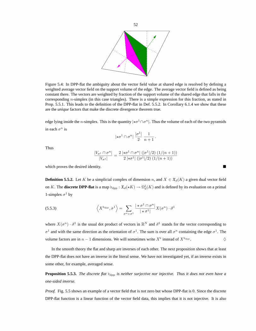
52
Figure 5.4: In DPP-flat the ambiguity about the vector field value at shared edge is resolved by defining aweighted average vector field on the support volume of the edge. The average vector field is defined as beingconstant there. The vectors are weighted by fraction of the support volume of the shared edge that falls in thecorrespondingn-simplex (in this case triangles). There is a simple expression for this fraction, as stated inProp. 5.5.1. This leads to the definition of the DPP-flat in Def. 5.5.2. In Corollary 6.1.4 we show that theseare theuniquefactors that make the discrete divergence theorem true.
edge lying inside then-simplex. This is the quantity|?σ1∩σn|. Thus the volume of each of the two pyramids
in eachσn is
|?σ1 ∩ σn| |σ1|2
1n+ 1
.
Thus|Vσ1 ∩ σn||Vσ1 |
=2 |?σ1 ∩ σn| (|σ1|/2) (1/(n+ 1))
2 |?σ1| (|σ1|/2) (1/(n+ 1))
which proves the desired identity.
Definition 5.5.2. LetK be a simplicial complex of dimensionn, andX ∈ Xd(K) a given dual vector field
onK. Thediscrete DPP-flatis a map[dpp : Xd(?K) → Ω1d(K) and is defined by its evaluation on a primal
1-simplexσ1 by
(5.5.3)⟨X[dpp , σ1
⟩=∑
σnσ1
| ? σ1 ∩ σn|| ? σ1|
X(σn) · ~σ1
whereX(σn) · ~σ1 is the usual dot product of vectors inRN and~σ1 stands for the vector corresponding to
σ1 and with the same direction as the orientation ofσ1. The sum is over allσn containing the edgeσ1. The
volume factors are inn− 1 dimensions. We will sometimes writeX[ instead ofX[dpp . ♦
In the smooth theory the flat and sharp are inverses of each other. The next proposition shows that at least
the DPP-flat does not have an inverse in the literal sense. We have not investigated yet, if an inverse exists in
some other, for example, averaged sense.
Proposition 5.5.3. The discrete flat[dpp is neither surjective nor injective. Thus it does not even have a
one-sided inverse.
Proof. Fig. 5.5 shows an example of a vector field that is not zero but whose DPP-flat is 0. Since the discrete
DPP-flat function is a linear function of the vector field data, this implies that it is not injective. It is also

53
Figure 5.5: A dual vector field that shows that the[dpp is not one-one. The arrows are based at circumcentersand are supposed to be of equal lengths and orthogonal to the corresponding outer boundary edge.
not surjective. Just consider an equilateral triangle and a 1-form that takes value 1 on each edge. There is no
vector field whose DPP-flat will give this 1-form.
5.6 Other Discrete Flats
Now we will discuss the remaining 7 types of discrete flats. For some we give the explicit expression and for
the more complicated ones we describe the construction in words.
PPP-flat: Barycentric interpolation inside ann-simplex reduces to barycentric interpolation along the
edge, i.e., linear interpolation along the edge. Thus we have forσ1 = [v0, v1]
⟨X[ppp , σ1
⟩=∫
σ1X · ~σ1
whereX is the linear interpolation of the valuesX(v0) andX(v1) alongσ1.
PPD-flat: Here the vectors at the vertices ofσn are linearly interpolated inside the simplex. IfX is this
interpolation then forσn−1 ≺ σn
⟨X[ppd , σ1
⟩=∫
σ1X · ?σn−1 .
PDP-flat: The vector field in Voronoi region of each vertex is constant. Thus forσ1 = [v0, v1]
⟨X[pdp , σ1
⟩= X(v0) ·
~σ1
2+X(v1) ·
~σ1
2
=X(v0) +X(v1)
2· ~σ1
and so the average value along the edge is used.

54
PDD-flat: Like the previous case, the interpolated vector field is constant in the Voronoi region of a
vertex. Letσn−1 ≺ σn and consider the dual edge?σn−1 where the flat is to be evaluated. This dual edge
intersectsσn−1 at the circumcenterc(σn−1). Thusevery pointon the dual edge is equidistant to every vertex
σ0 ≺ σn−1. Thus clearly the valuesX(σ0) should be combined with the same factor 1. Indeed this is also
the conclusion of Corollary 6.1.8 of the proof of primal discrete divergence theorem in Chapter 6. In other
words, a primal discrete divergence theorem is true if and only if PDD-flat is defined as below:
⟨X[pdd , ?σn−1
⟩:=
∑σ0≺σn−1
X(σ0) · (?σn−1)
where we have used?σn−1 to mean both the dual edge and the dual edge considered as a vector.
DPP-flat: This has been derived in the previous section.
DPD-flat: HereX is made constant inside ann-simplex. Let?σn−1 be the dual edge on which we want
to evaluate the flat. We define
⟨X[dpd , ?σ1
⟩=
∑σnσn−1
X(σn) · (?σn−1 ∩ σn)
where by abuse of notation,?σn−1 ∩ σn stands for the vector corresponding to the dual edge inσn.
DDP-flat andDDD-flat: These two require the new barycentric interpolation of Warren et al. [2003] and
we will not use them in this thesis.
5.7 A Primal-Dual Sharp for Exact Forms
As mentioned in Section 5.3 a proper development of the discrete flat operator should probably start with
interpolating the discrete 1-form data. The two choices for interpolation might be into the support volume,
and into the simplex by using Whitney forms of Section 3.3. We do not do that in this thesis, and instead, we
shortcut the process of interpolation and define 4 types of sharps based on 2 types of sources and 2 types of
destination. Of these we will only discuss PD-sharp for exact forms and PP-sharp.
To motivate the definition of primal-dual sharp for exact forms we do the following simple calculation of
gradient. Letf be the function that is obtained by linearly interpolating in ann-simplex the discrete 0-form
f . Thus for a pointx ∈ σn, using the interpolation functions we have that
f∣∣σn (x) =
∑σ0≺σn
f(σ0) φσ0,σn(x) .
55
Taking the usual gradient of this smooth function inIntσn we have
(5.7.1) (∇f)∣∣Int(σn)
=∑
σ0≺σn
f(σ0)∇φσ0,σn .
Let [v0, . . . , vn] = σn. Then by equation (2.7.2) we have that
∇φv0,σn = −∑
1≤i≤n
∇φvi,σn .
Substituting this into (5.7.1) we get
(∇f)∣∣Int(σn)
=∑
0≤i≤n
f(vi)∇φvi,σn
=∑
1≤i≤n
f(vi)∇φvi,σn −∑
1≤i≤n
f(v0)∇φvi,σn
=∑
1≤i≤n
(f(vi)− f(v0))∇φvi,σn .
Thus
(∇f)∣∣Int(σn)
=∑
1≤i≤n
(f(vi)− f(v0))∇φvi,σn .
Note that here the coefficientsf(vi) − f(v0) are nothing butd f evaluated on the edge[v0, vi]. Since
∇f = d f in the simplex interior, the above equation suggests the following definition for a primal-dual
sharp.
Definition 5.7.1. Let f be a discrete 0-form on a primal mesh,σn a simplex in this mesh andv a vertex of
σn. Then thediscrete primal-dual sharp for exact forms is defined by
(5.7.2)⟨(d f)]pd , ?σn
⟩:=
∑σ0≺σn
(f(σ0)− f(v))∇φσ0,σn .
We state without proof that the value is independent of whichv is chosen as the distinguished vertex. This is
clear from the calculation of gradient done above. A pictorial depiction of this formula is in Fig. 5.6.♦
We did not define the primal-dual sharp for general forms because in that case the choice of the vertex
v will in general, affect the answer. One could try to take all vertices ofσn one by one, and use some sort
of weighting, such as|?σ0 ∩ σn|/σn. Then in equation (5.7.2) above,f(σ0) − f(v) would be replaced by⟨α, [σ0, v]
⟩whereα is the discrete 1-form whose sharp is desired. However, this is an ad hoc weighting and
as we have been stressing, perhaps the right way to build discrete sharps is to first interpolate the discrete
1-forms, using, for example, Whitney maps.

56
Figure 5.6: The geometry of PD-sharp for exact forms. The color coding shows the values that are related.The arrows are gradients of primal-primal interpolation functions. The sum is taken at a vertex, any vertexwill do and will give the same result. The value of the exact form on each edges incident on that vertex isused.
5.8 A Primal-Primal Sharp
If we start with a primal 1-form and want to produce from it a primal vector field at a vertex, then one ad
hoc definition is to compute the sharp in each simplex of a one-ring around the vertex. This can be done
by using that vertex as the distinguished vertexv of equation (5.7.2) and using evaluations of the 1-form
on edges instead of evaluation ofd f in that equation. Then one can use some weighting for each simplex,
say the portion of the Voronoi region that falls in each simplex. Or, the fraction of volume that the simplex
represents, of the one-ring volume. The former choice would lead to the following definition. Unlike our
uniqueness result in the discrete flat case, we have not attempted any uniqueness proofs in discrete sharps,
since the future development will probably involve interpolation of 1-forms.
Definition 5.8.1. LetK be a flat simplicial complex of dimensionn and letα ∈ Ω1d(K) be a discrete primal
1-form. Thediscrete primal-primal sharp is ]pp : Ω1d(K) → Xd(K) (but we’ll just write]) and is defined
by its evaluation on a given vertexv as follows
(5.8.1) α](v) =∑
[v,σ0]
⟨α, [v, σ0]
⟩ ∑σn[v,σ0]
| ? v ∩ σn||σn|
∇φσ0,σn .
The outer sum is over all 1-simplices[v, σ0] containing the given vertexv and the inner sum is over allσn
containing the 1-simplex[v, σ0]. The volume factors are in dimensionn. The mapsφσ0,σn are the primal-
primal interpolation functions. A pictorial depiction is in Fig. 5.7. ♦
5.9 Composing Sharps and Flats
Note that[dpp goes from dual vector fields to primal 1-forms. But]pp goes from primal 1-forms to primal
vector fields. Thus although sharp and flat in the smooth theory are inverses, heretheseparticular the discrete
sharp and flats cannot be inverses of each other. We have see also in Prop. 5.5.3 that the DPP-flat cannot have
an inverse in the usual sense.
The incompatibility of domains and codomains for DPP-flat and PP-sharp seems similar to the incon-

57
Figure 5.7: The geometry of PP-sharp definition. The color coding shows the quantities that are related. Thearrows are the gradients of interpolation functions.
sistency of domains and ranges of mimetic div, grad, curl described on page 85 of Hyman and Shashkov
[1997a]. It is possible that analogous to the discrete Hodge star case some flats and sharps are inverses in
terms of averages but this is something we have not studied yet. Neither have we studied all possible com-
binations of discrete flats and sharps. We also note that we implicitly define a sharp and flat in Tong et al.
[2003] so thatdiv curl = 0 andcurl grad = 0. Although we do not use DEC formalism there, the above
result, which in exterior calculus is a consequence of sharp and flat being inverses of each other, is reproduced
in Section 9.3. ♦
5.10 Natural Pairing of Forms and Vector Fields
In the smooth theory pairing of forms and vector fields is a metric independent operation. At a point on the
smooth manifold, 1-forms are the usual linear algebraic duals of the vectors at that point. So the pairing is
just evaluation of the real-valued linear functions (1-forms) on the vector at that point.
Here we define the natural pairing of discrete 1-forms and vector fields that seems to depend on a metric.
After that we suggest how we may give a metric independent definition. We can use equation in Def. 5.2.1
which is the definition of] in the smooth case but now we use it as the definition of the natural pairing. This
gives us the following definition for discrete natural pairing.
Definition 5.10.1. LetK be a flat simplicial complex of dimensionn, α ∈ Ω1d(K) a discrete primal 1-form
andX ∈ Xd(K) a discrete primal vector field. Then theirdiscrete natural pairing, α(X) at a 0-simplexσ0
is defined as
α(X)(σ0) = α](σ0) · (X(σ0))
where· is the usual dot product in the embedding spaceRn. ♦
In future work we intend to consider interpolation of 1-forms using Whitney forms and also into the
support volumes of edges. Once the form is interpolated, one can use the smooth definition of pairing between

58
forms and vector fields to yield a discrete definition of pairing.
5.11 Summary and Discussion
The focus of this chapter has been the definition of sharps and flats. These are metric dependent operators that
were defined in the smooth theory, so that vector calculus could be brought under the umbrella of exterior
calculus. In this chapter we have made explicit the translation between discrete forms and discrete vector
fields using the metric information in specific, geometric formulas. In works on DEC that use vector fields
as proxies for forms, this is usually done implicitly by assuming flat space, and often even inR3. Our
development is explicit and general and works for non-flat meshes, when the choice of vector field and
interpolation scheme allows non-flatness. This allows one to define discrete vector calculus operators using
DEC. This is not essential for equations of mechanics, but it does help in discretizing equations that are
written in terms of div, grad and curl.
We have been able to define flats by using interpolation of vector fields which we treat as vector valued 0-
forms. For a proper definition of sharps it may be necessary to first interpolate 1-forms. Instead, here we gave
some ad hoc definitions. One drawback of these definitions is that the resulting definition of form-vector field
pairing is metric dependent. We also did not demonstrate a discrete sharp-flat inverse pair. In addition, we
showed that one of the discrete flats that we studied in detail cannot have an inverse in the usual sense. There
may be an inverse pair, or the inverse may exist in some kind of average manner. That is for future study.
Indirect evidence that such might be the case comes from our other work, on vector field decomposition in
which we have found vector calculus operators that satisfy the usual identities which are, in smooth theory, a
consequence of sharp and flat being inverses of each other and the fact thatd d = 0.

59
Chapter 6
Div, Grad, Curl and Laplace-Beltrami
Results: In smooth theory, divergence is defined in terms of the Lie derivative of a volume form. We
will define it first via an identity of exterior calculus involving flat operator. We show that we get a primal
and a dual discrete divergence theorem. Corollaries of the proofs of these also show that the factors in the
definition of DPP-flat and PDD-flat are unique. Also, in the 2D case our formula for discrete divergence is
the same as that appearing in other literature such as Polthier and Preuss [2002]. Then we briefly discuss
the other definition of divergence, based on derivative of volume. We define Laplace-de Rham operator,
of which, a special case is the Laplace-Beltrami of functions on manifolds. In a 2D calculation, our DEC
definition reproduces a well-known Laplace-Beltrami formula found in computer graphics by Meyer et al.
[2002]. The formula can also be derived variationally, using a DEC framework, as shown to us recently by
Castrillon Lopez and Fernandez Martinez [2003]. Our discrete gradient is defined using the PD-sharp for
exact forms from the previous chapter and another one using an averaging property of the PP-sharp. For curl
we show a 2D definition and a 3D definition and show that the 2D formula in DEC agrees, modulo an area
factor, with that found by Polthier and Preuss [2002].
Shortcomings: The definition of divergence involves two Hodge stars and a flat operator. It is an identity
in smooth theory that the metric inherent in these, finally enters the divergence formula only via the volume
form. We have not shown that the same is true in discrete theory. However we give some preliminary
comments on the volume based definition of divergence in this chapter. We have derived a 3D curl in our
other work in Tong et al. [2003] that satisfies all the usual vector calculus identities. But we have not yet
reproduced that definition via a DEC derivation. We think that the proper definitions of a general gradient
and 3D curl requires that the sharp operator be build from interpolation of 1-forms, like the flat was built from
interpolation of 0-forms.

60
6.1 Divergence
In the smooth theory, divergence is defined via a Lie derivative by(divX)µ = £Xµ whereµ is the volume
form associated with the given metric. In future work we plan to explore this definition in the discrete theory.
Some preliminary comments about this are given at the end of this section, in the context of Def. 6.1.9 where a
volume based definition is given. This volume based definition is the straightforward, intuitive interpretation
of the Lie derivative definition.
The main content of this section however, is the definition of a discrete divergence using an identity from
smooth theory. We don’t know yet if Lie derivative based definition and the present definition will turn out
to be identical. But we point out that the present flat based definition does result in a discrete divergence
theorem, for both primal and dual vector fields. This is the content of Theorem 6.1.3 and 6.1.7. First we
prove some lemmas that establish a discrete divergence theorem on a single dualn-cell and a single primal
n-simplex. Later we combine many dualn-cells or primaln-simplices to produce the divergence theorems.
Definition 6.1.1. For a discrete vector fieldX thediscrete divergence, div(X) is defined to be
div(X) := −δX[ = ∗d ∗X[ .
The above definition is actually a theorem in smooth exterior calculus and a consequence of the Lie derivative
based definition. See, for example, page 458 of Abraham et al. [1988]. IfX is a dual vector field, the discrete
flat used above is[dpp. For a primal vector field,[pdd is used. In other words ifX ∈ Xd(?K) then
(6.1.1)⟨div(X), σ0
⟩= ∗d ∗X[dpp
and ifX ∈ Xd(K) then
(6.1.2) 〈div(X), ?σn〉 = ∗d ∗X[pdd .
Thus for a dual vector field, divergence is a primal 0-form, and for a primal vector field divergence is a dual
0-form. ♦
The divergence defined as above satisfies a discrete divergence theorem. This is proved for a dual vector
field in the following lemma and theorem. For a primal vector field, we only sketch the proof. We will now
prove the discrete divergence theorem for dual vector fields over dualn-cells, starting with the result over a
single dualn-cell.
Lemma 6.1.2 (Divergence Theorem on a Dualn-cell). LetK be a primal mesh, not necessarily flat, and

61
of dimensionn, andσ0, a vertex in it. LetX ∈ Xd(?K) be a dual vector field on the complex. Then
(6.1.3) |?σ0| 〈div(X), σ0〉 =∑
σ1σ0
∑σnσ1
| ? σ1 ∩ σn|(X(?σn) · ~σ
1
|σ1|
).
where the edgesσ1 are oriented so that they all point outwards.
Proof. First we indicate why we call this a divergence theorem. Here~σ1/|σ1| is a unit normal perpendicular
to the boundary of the region?σ0 and pointing outwards. This region is the Voronoi region of the vertexσ0
wherediv(X) is being evaluated. The quantity| ? σ1 ∩ σn| is the length of the part of the dual edge ofσ1
that is in the simplexσn. Thus equation (6.1.3) is a statement of the divergence theorem over the Voronoi
region?σ0, i.e., the integral of divergence over this region equals the the flux ofX through the boundary of
this region.
In this proof we will write[ as a shorthand for[dpp. Sincediv(X) = ∗d ∗X[, as expected, the divergence
is a scalar. In particular because the flat used is DPP-flat andX is a dual vector field,X[ is a primal 1-form
and so due to the two Hodge stars,div(X) is a primal 0-form. Thus we can compute it at a primal vertex,σ0.
This is the quantity ⟨div(X), σ0
⟩=⟨∗d ∗X[, σ0
⟩.
Using the definition of Hodge star we get
1|σ0|
⟨∗d ∗X[, σ0
⟩=
1s |?σ0|
⟨∗ ∗ d ∗X[, ?σ0
⟩.
Heres is the sign± as discussed in the Hodge star definition for0- andn-simplices in Chapter 4. Assume,
without loss of generality, that the orientation ofK is the one that makess = (−1)n−1. Then, since|σ0| = 1,
we get
⟨div(X), σ0
⟩=
(−1)n−1
|?σ0|
⟨∗ ∗ d ∗X[, ?σ0
⟩=
(−1)n−1
|?σ0|
⟨d ∗X[, ?σ0
⟩=
(−1)n−1
|?σ0|
⟨∗X[, ∂(?σ0)
⟩.
The second equality is by application of definition of Hodge star and the last one above is by application of
discrete Stokes’ theorem. But by Def. 3.6.8 of dual boundary,
∂(?σ0) =∑
σ1σ0
?(sσ1σ1)
where the signsσ1 = ±1 is chosen to that the edgessσ1 σ1 all point inwards or outwards, depending on the
orientation ofK as explained Def. 3.6.8. In our case, the orientation has been chosen so that they will all

62
point outwards. See Def. 4.1.1 and Def. 3.6.8 for an explanation.
For simplicity of notation in the calculation that follows, we will useσ1 instead ofsσ1σ1. That is, we will
assume that the edgesσ1 have been oriented so that they all point outwards. Now we can use the linearity of
the pairing of forms and chains and write
(−1)n−1
|?σ0|
⟨∗X[, ∂(?σ0)
⟩=
(−1)n−1
|?σ0|
⟨∗X[,
∑σ1σ0
?σ1
⟩
=(−1)n−1
|?σ0|∑
σ1σ0
〈∗X[, ?σ1〉 .
Another use of the definition of discrete Hodge star now gives
1|?σ0|
∑σ1σ0
〈∗X[, ?σ1〉 =1
|?σ0|∑
σ1σ0
|?σ1||σ1|
〈X[, σ1〉 .
Now we can use the definition of DPP-flat operator and we get that
1|?σ0|
∑σ1σ0
|?σ1||σ1|
〈X[, σ1〉 =1
|?σ0|∑
σ1σ0
|?σ1||σ1|
∑σnσ1
| ? σ1 ∩ σn||?σ1|
X(?σn) · ~σ1(6.1.4)
=1
| ? σ0|∑
σ1σ0
∑σnσ1
| ? σ1 ∩ σn||σ1|
X(?σn) · ~σ1
=1
|?σ0|∑
σ1σ0
∑σnσ1
| ? σ1 ∩ σn|(X(?σn) · ~σ
1
|σ1|
)
whereσ1 all point outwards. Thus we have finally that
|?σ0| 〈div(X), σ0〉 =∑
σ1σ0
∑σnσ1
| ? σ1 ∩ σn|(X(?σn) · ~σ
1
|σ1|
)
which we wanted to show.
Theorem 6.1.3 (Divergence Theorem on a Dualn-Chain). Let c be a dualn-chain which, as a set, is a
simply connected subset of|K|. Then the discrete divergence theorem is true over this set.
Proof. It is enough to show that for two adjacent dualn-cells the contributions due to the shared dual edge
cancel in the RHS of equation (6.1.3). Consider two such adjacent dualn-cells. Letv0 andv1 be the two
vertices of which these are the dual cells. Since the cells are adjacent, there is an edge[v0, v1] and its
dual is the only shared face. That edge appears with opposite signs for the two versions of equation 6.1.3
corresponding tov0 andv1. The coefficients are otherwise the same. Thus the term corresponding to that
edge cancels.
Corollary 6.1.4 (Uniqueness of DPP-flat).The discrete divergence theorem on a dualn-cell is true if and
63
only if the factors in the DPP-flat definition, Def. 5.5.2, are
|?σ1 ∩ σn||?σ1|
.
Proof. Suppose in the proof of Lemma 6.1.2 above we replace the definition ofX[dpp in equation (6.1.4) by
one that uses arbitrary factorsbσn . Thus we have, in the proof of Lemma 6.1.2, that
⟨div(X), σ0
⟩=
1|?σ0|
∑σ1σ0
|?σ1||σ1|
∑σnσ1
bσnX(?σn) · ~σ1
=1
|?σ0|∑
σ1σ0
∑σnσ1
|?σ1|bσn
(X(?σn) · ~σ
1
|σ1|
).
Since the divergence theorem must be true for any dual vector fieldX we can choose one which is 0 every-
where except in oneσn σ0. Then the divergence theorem is true iff|?σ1 ∩ σn| = |?σ1|bσn for some
σ1 ≺ σn, which implies that
bσn =| ? σ1 ∩ σn|
|σ1|.
Sinceσn was arbitrary, this proves the desired uniqueness.
Remark 6.1.5. Divergence of dual vector field in primal is 0: If divergence is computed by Def. 6.1.1,
for a dual vector field inside a primaln-simplex, the DPD-flat is used. An easy calculation shows that then
the divergence at the center of the simplex is 0, because in the calculation, there is a sum of the dot product
of a vector with the dual edges which are scaled so that the sum is 0. Thus one gets the correct answer in this
case. To compute the divergence inside a primal simplex but for a primal vector field, one uses a PDD-flat
and this results in the following Lemma. ♦
Lemma 6.1.6 (Divergence Theorem on a Primaln-simplex). LetK be a flat primal mesh of dimensionn,
andσ0 a vertex in it. LetX ∈ Xd(K) be a primal vector field on the complex. Then
(6.1.5) |σn| 〈div(X), ?σn〉 =∑
σn−1≺σn
|σn−1|
( ∑σ0≺σn−1
X(σ0)
)· ?σ
n−1
|?σn−1|.
where the orientation ofσn is such that the dual edges?σn−1 point outwards. If the given orientation is the
other one then RHS is multiplied by−1.
Sketch of proof.The proof consists of application of the definitions, as in the proof of Lemma 6.1.2. The
only difference is that PDD-flat is used. Thus the vector field is interpolated to be constant in the Voronoi
dual of each primal vertex.
Theorem 6.1.7 (Divergence Theorem on a Primaln-chain). Let c be a primaln-chain which, as a set, is
a simply connected subset of|K|. Then the discrete divergence theorem is true over this set.

64
Sketch of proof.It is enough to show this for two adjacent primaln-simplices. It follows due to the fact that
the shared face is oriented oppositely by the adjacent simplices while the vector field data is the same. This
causes a cancellation giving us the proof over the two simplices.
Corollary 6.1.8 (Uniqueness of PDD-flat).The discrete divergence theorem on a primaln-simplex is true
if and only if the factors in the PDD-flat definition in Section 5.6 are 1.
Proof. Similar to the proof of Cor. 6.1.4.
Now we will give the formal definition of divergence via the volume form. We have not worked out the
resulting discrete formula in all cases, but in 2D, it appears to give the same result as the definition used
above.
Definition 6.1.9. LetX be a discrete primal vector field on a flat complexK andσ0 a vertex inK. Extend
X to X in anysmooth fashion to a neighborhood of the boundary vertices of the one-ringSt(σ0) aroundσ0.
Then the discrete divergence on the one-ring is defined by
⟨div(X), σ0
⟩|St(σ0)| := d
dt
∣∣∣∣t=0
|ϕt(St(σ0))|
whereϕt is the affine simplicial homeomorphism extended from from the flow ofX restricted to the ver-
tices. ♦
We intend to explore this definition in future work. The nice property of this is that the metric enters only
via the volume form as it should.
6.2 Gradient
In smooth theory the gradient of a function is(d f)]. Thus it converts the metric independent quantity into
a metric dependent one. For a primal 0-form the gradient can easily be computed in the interior of the
primal simplex by first interpolating the 0-form from the vertices to the interior using the affine, barycentric
interpolation functions, and then taking the gradient. Since the interpolation is affine, the gradient is a constant
vector and we can associate it with the dual of the simplex. This is the primal-dual gradient defined below.
For the primal-primal gradient, one has to necessarily combine the information from the one ring around a
vertex in some way, and for now we propose an ad hoc method using the primal-primal sharp.
As we mentioned in Section 5.8, the right way to define sharp is to interpolate 1-forms first. But we have
not done that in this thesis, and instead we have given an ad hoc definition. Similarly one can give ad hoc
definitions for dual-dual and dual-primal sharps and consequently for those gradients. But we will not do
that here. In summary, the only reliable gradient we give here is the obvious one, the primal-dual gradient.
We note however, that our primal-primal gradient, when interpreted for regular nonsimplicial 2D rectangular

65
mesh, gives a standard, finite difference formula for the gradient. The primal-dual and primal-primal gradients
are defined below.
Definition 6.2.1. Let K be a primal mesh of dimensionn andf ∈ Ω0d(K) a discrete primal 0-form, i.e., a
real valued function on the vertices ofK. Then thediscrete primal-dual gradient of f writtengradpd f or
∇pdf is defined as(df)]pd . That is, using Definition 5.7.1 of discrete] its value on?σn is:
(6.2.1)⟨(d f)]pd , ?σn
⟩:=
∑σ0≺σn
(f(σ0)− f(v))∇φσ0,σn
wherev is a vertex ofσn and we state without proof that the definition is independent of whichv is chosen.
Given a vertexv ∈ K thediscrete primal-primal gradient of f is defined as(d f)]pp by
(6.2.2) (∇ppf)(v) :=∑
σ1=[v,σ0]
[f(σ0)− f(v)
] ∑σn[v,σ0]
|?v ∩ σn||σn|
∇φσ0,σn .
The outer sum is over all 1-simplices[v, σ0] containing the given vertexv and the inner sum is over allσn
containing the 1-simplex[v, σ0]. The volume factors are in dimensionn. The mapsφσ0,σn are the primal-
primal interpolation functions. ♦
6.3 Curl
In vector calculus, curl is usually defined in dimension 3 and sometimes as a scalar in dimension 2. In the
smooth exterior calculus notation these are,∗dX[ in dimension 2 and(∗dX[)] in dimension 3, whereX
is a smooth vector field inR2 or R3 respectively. In geometric mechanics the use of curl may be replaced
by d of a 1-form. One example is vorticity in fluid mechanics, which isdu[ in geometric theory of fluid
mechanics, butcurlu in the more common engineering literature. Notice that the sharp is not required in the
geometric mechanics definition of vorticity. In any case, having a discrete curl in exterior calculus is useful
for translating equations that have been written using curl. Due to the multiplicity of discrete sharps and flats
there will be many definitions of discrete curls. We have not explored all these, and give only one definition
each in the 2D and 3D case.
We first define the 2D curl and show that the DEC definition results in the same formula, modulo an area
factor, as one found by Polthier and Preuss [2002]. This is the content of Rem. 6.3.2.
Definition 6.3.1. Let K be a primal mesh of dimension 2 andX ∈ Xd(?K) a dual vector field. Then the
discrete 2D dual-primal curl is defined by
curldpX = ∗dX[dpd .

66
O
AC
PQ
B
Figure 6.1: Curl in 2D
Remark 6.3.2. DEC 2D curl compared to Polthier and Preuss [2002]: The DEC definition of the 2D
dual-primal curl coincides with one found by Polthier and Preuss [2002], modulo an area factor that their
definition does not have. Consider the configuration shown in Fig. 6.1. According to Polthier and Preuss
[2002], the discrete curl in 2D that assigns vectors to primal nodes is
⟨curl(X), σ0
⟩=
12
∑σ2σ0
X(?σ2) · ~σ1(σ2)
whereσ1(σ2) is the outer edge of triangleσ2. Let us compute the DEC version of the 2D curl. For simplicity
of notation we will use[ instead of[dpd. Since∗dX[ is a 0-form, we can evaluate it at a vertexσ0. In
Fig. 6.1 this is marked as the pointO whose one-ring is shown in that figure. Let the complex shown in the
figure be oriented by orienting each triangle counter clockwise. By definition of discrete Hodge star we have
1σ0
⟨?dX[, σ0
⟩=
1−|?σ0|
⟨dX[, ?σ0
⟩.
Then, by discrete Stokes’ theorem we have
⟨curlX,σ0
⟩=
1−|?σ0|
⟨X[, ∂(?σ0)
⟩.
By the definition of dual boundary, and because of the orientation chosen for the complex we get
⟨curlX,σ0
⟩=
1|?σ0|
∑σ1σ0
⟨X[, ∂(?σ0)
⟩
where the negative sign has canceled with the one coming from the dual boundary definition and all theσ1
are pointing outwards.
The flat to be used is the DPD-flat. This consists of simply taking the dot product of the vector inside
each triangle with the dual edges, when evaluatingX[ on the dual edges. This is because in DPD-flat the dual

67
vector field inside the triangle is interpolated to be constant inside the triangle. Thus the above RHS becomes
1|?σ0|
∑σ1
∑σ2σ1
X(?σ2) · (?σ1 ∩ σ2) .
Collecting terms by the triangles we get
⟨curlX,σ0
⟩=
1|?σ0|
∑σ2σ0
∑σ1≺σ2
X(?σ2) · (?σ1 ∩ σ2) .
In the case of the triangle shown with the dual edges in Fig. 6.1, the term∑
σ1≺σ2 X(?σ2) · (?σ1 ∩ σ2) in
the RHS above becomes simply
X(B) ·−−→AB +X(B) ·
−−→BC .
The term according to Polthier and Preuss [2002] should be
12X(B) ·
−−→PQ .
But
X(B) ·−−→AB +X(B) ·
−−→BC = X(B) · (
−−→AB +
−−→BC) = X(B) ·
−→AC =
12X(B) ·
−−→PQ
where the last equality is due to the elementary geometric fact that the length of the edge joining midpoints
of two sides is half the remaining side of the triangle and in the same direction as it. Thus the DEC formula is
the same as the one given in Polthier and Preuss [2002] except that we have an additional factor of1/|?σ0|. ♦
For the 3D curl one needs to define sharp operator. We have given a primal-dual sharp for exact forms
and a primal-primal sharp in Chapter 5. Of these, only the primal-dual sharp for exact forms is satisfactory.
Thus the correct formulation of 3D discrete curl will have to wait a better development of sharp, which will
possibly involve interpolation of 1-forms. For completeness we give here the definition of a discrete 3D curl
using the usual smooth exterior calculus definition of curl.
Definition 6.3.3. LetK be a flat simplicial complex of dimension 3. LetX ∈ Xd(K) be a discrete primal
vector field. Then thediscrete 3D curl is defined by
curl(X) = (∗d(X[))]
where the operators∗, [ and] on RHS are the discrete operators. ♦
Remark 6.3.4. Curl and vector calculus identities: Recall that in smooth exterior calculus the identity
div curl = 0 follows from the fact thatd2 = 0. This is becausediv(curl(X)) = d ∗ ([∗(dX[)]][) and]
is the inverse of[. However as we pointed out in Section 5.9, in the discrete case we have to use the right
combination of] and[. For example, in this chapter we have used a dual-primal flat and a primal-primal

68
iβij
α ijx j
x
Figure 6.2: The variable names used in formula (6.4.1) for the Laplace-Beltrami of a triangle mesh, found byMeyer et al. [2002]. The complex does not have to be flat.
sharp. The composition has no chance of being identity. We point out that various vector calculus identities
are true in our vector field decomposition work Tong et al. [2003]. The proof is reproduced in Section 9.3.
Thus the information about the right flat and sharp to use is probably hidden in that work. ♦
6.4 Laplace-Beltrami
The Laplace-Beltrami operator is the generalization to curved surfaces, of the usual Laplacian of flat space.
In the smooth case the Laplace-Beltrami operator on smooth functions is defined to be∇2 = div curl = δd.
See, for example, page 459 of Abraham et al. [1988]. In the smooth case the Laplace-Beltrami on functions is
a special case of the more general Laplace-deRham operator∆ : Ωk(M) → Ωk(M) defined by∆ = dδ+δd.
In this section we show that this definition of Laplace-Beltrami leads to a well-known formula for discrete
Laplace-Beltrami found by Meyer et al. [2002]. The formula that they found was
(6.4.1) ∆f(xi) =1
2A∑
j∈N1(i)
(cot αij + cot βij) (f(xi)− f(xj))
where the angles and points shown are marked in Fig. 6.2. The termA stands for an area around the pointxi.
Meyer et al. [2002] also showed that the use of the Voronoi area around the vertex is optimal in some sense.
Recently, Castrillon Lopez and Fernandez Martinez [2003] showed us that the Laplace-Beltrami we derive
can be obtained from a discrete variational principle, by extremizing a discrete Dirichlet energy. This shows
that, at least in this case of harmonic maps, discretizing the smooth Lagrangian and obtaining the discrete
Euler-Lagrange equations gives the same result as first obtaining the Euler-Lagrange equations and then
discretizing them. Thus in this case the application of variational principle commutes with discretization via
DEC.
Example 6.4.1. Laplace-Beltrami on a triangle mesh:As an example we compute here∆f on a primal
vertexσ0 wheref ∈ Ω0d(K) andK is a (not necessarily flat) triangle mesh inR3. Suppose thatK is oriented

69
by orienting all its triangles counterclockwise. Sinceδf = 0 by definition, we have that
⟨∆f, σ0
⟩=⟨δdf, σ0
⟩= −
⟨∗d ∗ df, σ0
⟩.
Now by using the definition of discrete Hodge star followed by the discrete Stokes’ theorem we get
⟨∗d ∗ df, σ0
⟩=
|σ0|−|?σ0|
⟨d ∗ df, ?σ0
⟩=
−1|?σ0|
⟨∗df, ∂(?σ0)
⟩.
The explanation for the use of signed volume−|?σ0| was given in Rem. 4.1.2. Thus
⟨∆f, σ0
⟩=
1|?σ0|
⟨∗df, ∂(?σ0)
⟩.
By Def. 3.6.8 of the dual boundary,
∂(?σ0) =∑
σ1σ0
?(sσ1σ1)
wheresσ1 = ±1 is a sign, that depends on the orientation ofK andσ1. In dimension 2, with triangles of
K oriented counterclockwise, the definition of dual boundary dictates that the edgessσ1σ1 are all pointing
outwards. For simplicity, as usual, in the following we will setσ1 to besσ1 σ1, which means that all edges
incident onσ0 are now all pointing outwards. Thus,
⟨∗df, ∂(?σ0)
⟩=
⟨∗df,
∑σ1σ0
?σ1
⟩
=∑
σ1σ0
⟨∗df, ?σ1
⟩.
Now another use of the definition of discrete Hodge star gives
⟨∗df, ?σ1
⟩=|?σ1||σ1|
⟨df, σ1
⟩.
But then by discrete Stokes’ theorem we have that
⟨df, σ1
⟩= f(v)− f(σ0)
whereσ1 = [σ0, v]. Putting all this together we get that
(6.4.2)⟨∆f, σ0
⟩=
1|?σ0|
∑σ1=[σ0,v]
|?σ1||σ1|
(f(v)− f(σ0)) .

70
Then a geometric calculation shows that the above expression is the same as the formula (6.4.1) found by
Meyer et al. [2002], without using discrete exterior calculus. As mentioned before, this formula is also ob-
tained by a discrete variational principle as shown to us recently by Castrillon Lopez and Fernandez Martinez
[2003].
6.5 Summary and Discussion
In our future work the divergence will be defined via the Lie derivative of the volume form, as outlined in
Def. 6.1.9. For such a development, the vector field is extended in any smooth fashion, to the neighborhood
of vertices, and the mesh is moved with the flow of the vector field. The vectors can actually be placed at
any point, not just at the dual or primal vertices. Of course, then one would have to decide, what volume is
being used in that case – for example the convex hull of the points. If the vectors are placed at the primal
vertices, this definition of divergence can be pursued even in the current setting of DEC, without interpolation
of forms, since the volume form is defined everywhere. In hindsight, this is really the approach to divergence
we should have taken, since the metric dependence of divergence should only be through the volume form.
It should not have anything to do with Hodge duality, dual meshes or flat operator. The definition we used,
should actually be a theorem in the new setting.
In the interpolation view of DEC that we envision in the future, and as outlined in Section 1.5, the sharp
would be defined after interpolating 1-forms. This should yield a better definition of the 3D curl, that satisfies
various vector calculus identities. Similarly, that should yield a better primal-primal gradient, since in the
interpolation point of view, operators are defined even pointwise.
That said, we should point out that the definition of divergence we have given yields a nice divergence
theorem. Also, the formula in dimension 2, seems to be the same as the one obtained by the new, change of
volume point of view of divergence outlined above. The 2D curl we derive has been found by others, without
the use of DEC. The primal-dual gradient is a good definition, it even uses the idea of interpolation and the
primal-primal gradient yields a gradient on regular nonsimplicial meshes, as shown in Section 9.4.

71
Chapter 7
Wedge Product
Results: As in the smooth case, the discrete wedge product we will construct is a way to build higher
degree forms from lower degree ones. Some common applications of the wedge are, for example in defining
the Lagrangian for harmonic maps, asd f ∧∗d f . In spacetime electromagnetism in vacuum, starting with a
1-formA one defines the Lagrangian usingdA ∧ ∗dA. Thus the wedge product is of practical significance
in important applications. In this thesis we give two different definitions for the primal-primal wedge, one of
which is due to Castrillon Lopez [2003], and we state some of the properties that our primal-primal wedge
satisfies.
Shortcomings: For a complete treatment, the dual-dual and primal-dual discrete wedge products should
be defined. We only give speculative suggestions for the other cases here. One definition of primal-primal
wedge we give, uses the metric. This use of metric is not satisfying because in the smooth theory, the
definition does not use the metric. Furthermore, the discrete wedge should commute with discrete pullbacks.
The metric dependent definition doesn’t. Recently Castrillon Lopez [2003] showed us a definition of discrete
wedge which does not use the metricand which commutes with discrete pullbacks. We include it here for
completeness.
7.1 Primal-Primal Wedge
For information about the smooth case see the first few pages of Chapter 6 of Abraham et al. [1988]. We give
two definitions of a primal-primal wedge here. The first definition is the one we had been working with until
recently. The second definition was suggested to us recently by Marco Castrillion and it has the nice property
that it is natural under pullbacks, i.e., his definition commutes with discrete pullbacks. This is an example of
how naturality under pullbacks can be used as a criterion for selecting definitions in the discrete case, even
when the operator being defined, like the wedge, is on only one manifold. The other obvious advantage of
his definition is that metric is not used in the definition. His definition is Def. 7.2.1.

72
Definition 7.1.1. Given a primal discretek form αk ∈ Ωkd(K) and a primal discretel form βl ∈ Ωl
d(K) the
discrete primal-primal wedge product ∧ : Ωkd(K) × Ωl
d(K) → Ωk+ld (K) defined by the evaluation on a
k + l simplexσk+l = [v0, . . . , vk+l] as follows,
(7.1.1)⟨αk ∧ βl, σk+l
⟩:=
1(k + l)!
∑τ∈Sk+l+1
sign(τ)|σk+l ∩ ?vτ(k)|
|σk+l|(α ^ β)(τ(σk+l))
whereSk+l+1 is the permutation group and its elements are thought of as permutations of the numbers
0, . . . , k + l. Here sign(τ) is the sign of the permutationτ , being+1 if τ is even and−1 if it is odd.
The notationτ(σk+l) stands for the simplex[vτ(0), . . . , vτ(k+l)]. Finally the notation(α ^ β)(τ(σk+l)) is
borrowed from algebraic topology (see, for example, page 206 of Hatcher [2002]) and is defined as
(α ^ β)(τ(σk+l)) := 〈α,[vτ(0), . . . , vτ(k)
]〉〈β,
[vτ(k), . . . , vτ(k+l)
]〉 .
♦
The above expression looks complicated but the idea behind it, and its computation is really simple. What
it amounts to, is evaluating the formsα andβ on thek andl simplices emanating from each vertex of the
simplexσk+l on which the wedge product is being evaluated. The sign of the permutationτ is there to
provide the anti commutativity property. The volume factor is provided to make the computation democratic,
by giving an appropriate weight to each vertex ofσk+l. The following example of wedge product between
two 1-forms should clarify the notation.
Example 7.1.2. Let α andβ be two 1-forms whose wedge product has to be computed, sok = l = 1.
The definition above gives the value ofα ∧ β on a triangleσ2 = [v0, v1, v2]. According to the definition
above the permutation group to be used isS1+1+1 = S3. Thusτ are elements of the set of permutations of
0, 1, 2. We will write the elements ofS3 as 1-0-2, 2-0-1, 0-1-2, 2-1-0, 1-2-0 and 0-2-1 with the obvious
interpretation. The signs of these are−, +, +, −, + and− respectively. Let the volume factors appearing
in (7.1.1) be denoted byC0, C1 andC2, i.e., let
Ci =|σ2 ∩ ?vi||σ2|
.
Then
(7.1.2) 〈α ∧ β, [v0, v1, v2]〉 =12[−C0〈α, [v1, v0]〉〈β, [v0, v2]〉+ C0〈α, [v2, v0]〉〈β, [v0, v1]〉
+ C1〈α, [v0, v1]〉〈β, [v1, v2]〉 − C1〈α, [v2, v1]〉〈β, [v1, v0]〉
− C2〈α, [v0, v2]〉〈β, [v2, v1]〉+ C2〈α, [v1, v2]〉〈β, [v2, v0]〉]
Thus the formula says to go around the 3 vertices of the triangle evaluatingα and β on the two edges

73
α
βFigure 7.1: Pictorial depiction of 1 term in the sum in equation (7.1.2).
emanating from the vertex, then switching the arguments with an appropriate sign. The weighting factor is
the area of the triangle corner obtained by intersecting the Voronoi cell of the vertex with the triangle divided
by the area of the triangle. A pictorial depiction of 1 term in the equation above is in Fig. 7.1.
The definition Def. 7.1.1 discussed above has some nice properties and some undesirable properties. If
a smooth volumek-form and a volumel-form are discretized and their primal-primal wedge computed on a
(k + l)-simplex, the result is the volume of the simplex. Also, this wedge satisfies most of the properties of
the smooth wedge. Specifically the following lemma is true.
Lemma 7.1.3. The discrete wedge product∧ : Ωkd(K)×Ωl
d(K) → Ωk+ld (K) satisfies the following proper-
ties:
(i) Anti-commutativity αk ∧ βk = (−1)klβl ∧ αk.
(ii) Leibniz rule d(αk ∧ βl) = (dαk) ∧ βl + (−1)kαk ∧ (dβl).
(iii) Associativity for closed formsFor αk ∈ Ωkd(K), βl ∈ Ωl
d(K), γm ∈ Ωmd (K), such thatdαk = 0,
dβl = 0, dγm = 0, we have that,(αk ∧ βl) ∧ γm = αk ∧ (βl ∧ γm).
Proof. See Desbrun et al. [2003].
Remark 7.1.4. Lack of associativity: According to Givental [2003] this lack of associativity in general,
and a special status for closed forms, is not an accident. Putting the “democratic weighting” aside, the wedge
definition works for any simplicial complex (such as singular cochains, for instance). It is known that it is
in principal impossible to make a universal definition anti-commutativeand associative. This phenomenon
has been studied a lot in algebraic topology or homological algebra and gives rise to the concepts of Massey
products and homotopy-associative algebras.
In our situation, one can define on the chain complex(C∗,d) a sequence of operations: the binary
operationa, b 7→ ab (the wedge product), some triple operationa, b, c 7→ [a, b, c] etc. such that the deviation
of each operation from some kind of associativity property is measured by the differential of the previous
operation. The key example is:
(ab)c− a(bc) = d[a, b, c]− [d a, b, c]− [a,d b, c]− [a, b,d c] .

74
The signs correspond to evena, b, c and in general should be changed by the factors
(−1)deg(a) and(−1)deg(a)+deg(b)
in the last two summands. This implies that the product is associative on the cohomology i.e. whena, b, c
are closed, then(ab)c− a(bc) is exact. Our statement that it is not just exact but 0 is a bit surprising but not
impossible in this context. ♦
Remark 7.1.5. Wedge product and interpolation of forms: It has been pointed out by Sen et al. [2000]
that if the wedge product is defined by first interpolating the discrete forms by using the Whitney maps, the
resulting wedge product is still non-associative. Intuitively, this lack of associativity, and the lack in our case,
stem from the fact that one is not defining the wedge product pointwise. Thus it seems that one must not only
interpolate, but also specify, say, a vertex at which the evaluation must take place, to have a good chance of
getting associativity. This point of view seems to appear in Hiptmair [2002a] and we intend to explore this in
future work. ♦
Remark 7.1.6. Absence of naturality under pullback: Consider a simplexσn and an affine mapϕ : Rn →
Rn. Then in general the circumcenter isnot invariant under such maps. That is, in generalϕ(c(σn)) 6=
c(ϕ(σn)). Now suppose that we are given two simplicial complexes with a simplicial homeomorphismϕ
between them. If we use Def. 7.1.1 for the wedge then in general the wedge will not commute under discrete
pullback. That is, in general we willnot have that
〈ϕ∗(α ∧ β), σ〉 = 〈α ∧ β, ϕ(σ)〉 .
This appears to be not a good sign for that discrete definition, since the above property in the smooth theory
should follow from the change of variables theorem. Fortunately, the alternative definition presented in the
next section does satisfy this property. ♦
7.2 Alternative Primal-Primal Wedge
Now we give the other definition of primal-primal wedge, shown to us recently by Castrillon Lopez [2003],
which has the nice properties of not using the metric and of being natural under discrete pullbacks.
Definition 7.2.1 (Castrillon Lopez [2003]). Given a primal discretek form αk ∈ Ωkd(K) and a primal
discretel form βl ∈ Ωld(K) the natural (in the sense of commuting with discrete pullbacks)discrete primal-
primal wedge product ∧ : Ωkd(K) × Ωl
d(K) → Ωk+ld (K) defined by the evaluation on ak + l simplex
σk+l = [v0, . . . , vk+l] as follows,
(7.2.1)⟨αk ∧ βl, σk+l
⟩:=
1(k + l + 1)!
∑τ∈Sk+l+1
sign(τ)(α ^ β)(τ(σk+l)) .

75
♦
Remark 7.2.2. Comparison of factors: In the above definition, equation (7.2.1) can be rewritten as
⟨αk ∧ βl, σk+l
⟩=
1(k + l + 1)(k + l)!
∑τ∈Sk+l+1
sign(τ)(α ^ β)(τ(σk+l))
=1
(k + l)!
∑τ∈Sk+l+1
sign(τ)1
k + l + 1(α ^ β)(τ(σk+l)) .
Comparing this with equation (7.1.1) we find that the factor
|σk+l ∩ ?vτ(k)||σk+l|
in that definition has been replaced by1
k + l + 1.
Thus a metric dependent factor has been changed into a constant factor. This is what makes Def. 7.2.1 natural
under discrete pullback. Note also that
∑τ∈Sk+l+1
|σk+l ∩ ?vτ(k)||σk+l|
=∑
τ∈Sk+l+1
1(k + l + 1)!
= 1
a property that is useful in proving properties of the discrete wedge. ♦
7.3 Summary and Discussion
In the last two sections we have discussed the primal-primal wedge product in some detail. We defined it
in two ways, one of which due to Castrillon Lopez [2003] has the nice feature of being defined without the
use of metric and of commuting with discrete pullbacks. Since forms can be dual as well, for a complete
treatment of discrete wedge product we should define dual-dual and primal-dual wedges. In this section we
give only some preliminary suggestions for these definitions and do not study the properties of these wedge
products.
Given a dual discretek form αk ∈ Ωkd(?K) and a dual discretel form βl ∈ Ωl
d(?K) thediscrete dual-
dual wedge product∧ : Ωkd(?K)×Ωl
d(?K) → Ωk+ld (?K) might be defined (modulo some factors that have
been left out) by the evaluation on ak + l dual cellσk+l = ?σn−k−l = ?[v0, . . . , vn−k−l] as follows.
〈αk ∧ βl, σk+l〉 =〈αk ∧ βl, ?σn−k−l〉
=∑
σnσn−k−l
sgn(σn−k−l, [vk+l, . . . , vn])∑
τ∈Sk+l
sign(τ)
· 〈αk, ?[vτ(0), . . . , vτ(l−1), vk+l, . . . , vn]〉〈βl, ?[vτ(l), . . . , vτ(k+l−1), vk+l, . . . , vn]〉

76
whereσn = [v0, . . . , vn], and we have without loss of generality assumed thatσn−k−l = ±[vk+l, . . . , vn].
Here we have left out the factor to be used, and that is for future work.
As mentioned in the preamble of this chapter, in some important applications, the Lagrangian can be
written asα ∧ ∗α. These are a complementary primal-dual pair, i.e., their degrees sum ton. The cochain
obtained by such a wedge product of ak and(n− k)-form could be defined on the support volumes of all the
k-simplices. Recall that these tile the underlying space|K|.
Let αk ∈ Ωkd(K) be a primalk-form andβn−k ∈ Ωn−k
d (?K) a dual(n − k)-form. Thusα andβ are
a complementary primal-dual pair. Thediscrete primal-dual wedge product∧ : Ωkd(K) × Ωn−k
d (?K) →
Ωnd (Vk(K)) can be defined by the evaluation on the support volume of ak-simplex as follows. Here
Ωnd (Vk(K)) are the cochains on then-cells that are the support volumes ofk-simplices. The value of
⟨αk ∧ βn−k, Vσk
⟩will likely involve terms like ⟨
αk, σk⟩ ⟨
β, ?σk⟩.
One obvious weighting factor to use for such a term might be
12
1n |σ
k| |?σk ∩ σn|Vσk
.
Here the numerator is the volume of that part of support volumeVσk that is formed byσk and its dual and
lies inside someσn. But again these factors are metric dependent, which may not be good.
However, recently Castrillon Lopez and Fernandez Martinez [2003] used a similar construction in the
special case ofn = 2 andk = 1 to do a discrete variational derivation of the Euler-Lagrange equation for
d f ∧ ∗d f . The solutions of these are harmonic maps on a surface. Their variational derivation yielded the
same Laplace-Beltrami operator that we defined in Chapter 6. They have shown that starting from a smooth
Lagrangian, one can derive the equation for harmonic maps and discretize it, or discretize the Lagrangian
and derive the discrete equation for harmonic maps using DEC. In both cases the resulting discrete Euler-
Lagrange equations are the same.

77
Chapter 8
Interior Product and Lie Derivative
Results: In this thesis, we are trying to build a discrete exterior calculus which treats vector fields and
forms as separate entities, as does smooth theory. One motivation is that Lie derivatives of forms and vector
fields are two very different things. This is expanded upon in Sec. 8.1 below. In this chapter we will discuss
interior product and Lie derivatives of forms. First, we will derive an identity relating smooth interior product
to Hodge star and wedge products. This yields an algebraic, discrete interior product. However since in
the discrete theory we are only concerned with integrals of forms we can use the notion of extrusion of a
manifold by the flow of a vector field to define integral of interior product. This is an idea of Bossavit [2003]
and it leads to another definition of discrete interior product. A similar distinction exists in our discrete Lie
derivative definition. Use of the Cartan homotopy formula leads to an algebraic definition of Lie derivative,
and a flow-out formula that we prove, leads to another, flow based definition. In this Chapter we argue that
interpolation of forms becomes a must for a proper definition of Lie derivative.
Shortcomings: Our algebraic definition of interior product uses metric information in the form of Hodge
star and flat. We prove here that in the smooth case this metric dependence cancels out. But we don’t know
if this cancellation happens in the discrete case also. We have not studied carefully which properties are
satisfied by the two definitions of interior product we give here. Nor have we studied if the two are the same
in the discrete case.
A wedge product is involved in the algebraic definition. Thus the Lie derivative of a wedge product
ends up with a wedge of three forms, if the algebraic definition is used. Due to the lack of associativity for
general forms, one risks losing the important property of Leibniz rule for Lie derivative, except perhaps, for
closed forms. This was pointed out to us by Alan Weinstein. We give here the discrete version of the flow-
out formula for Lie derivative, to the extent possible without interpolation of forms. This is one of the key
examples that shows the importance of interpolation of forms. In fact Bossavit [2003] uses the interpolation
approach approach for interior product. But we haven’t seen a Lie derivative development like this. Neither
have the properties of such an interior product been studied in detail.
The smooth definition of Lie derivative, and hence this interpolated one, depends on derivatives. Hence,

78
ultimately, the discrete definition for higher degree forms may turn out to be independent of the extension
(interpolation) used. Finally, we do not discuss the Lie derivatives of vector fields at all in this thesis.
8.1 Separation of Forms and Vector Fields
In Chapter 5 we defined discrete vector fields and the discrete sharps and flats for going between 1-forms and
vector fields. One use for sharps and flats is of course, to be able to translate vector calculus into exterior
calculus, allowing one to discretize equations written in vector calculus notation. But there is another, more
important reason for defining sharps and flats. As mentioned in Chapter 5, this is that in mechanics some
quantities aredefinedusing these operators. An example from Chapter 5 worth repeating for emphasis, is that
of vorticity in fluid mechanics. In geometric treatment of fluid mechanics vorticity is defined asdu[. Hereu
is the velocity field of the fluid, a genuine vector field which is not a proxy for a 1-form.
In many applied fields, vector calculus has been given prominence over differential forms even when
forms would have been more appropriate and simpler to use. In 3D, time-dependent electromagnetism,
the quantities of interest should be modeled by differential forms, not vector fields. When the Maxwell
system is written like this, theonly place where metric plays a role, is in the constitutive, material dependent
relationshipsd = ∗εe andb = ∗µ, wheree andh are 1-forms andd andb are two forms. When Maxwell’s
equations are written in terms of vector fields, which is the more common formulation, thenall the fields that
appear are proxies for 1-forms and 2-forms.
In R3, this prevalent confusion between 1-forms, 2-forms and vector fields, all of which have a basis size
of 3, takes the following form. For example, given a vector fieldF onR3 given by
F = F1∂
∂x+ F2
∂
∂y+ F3
∂
∂z
we can identify it with the 1-formF [ = F1dx + F2dy + F3dz. With the standard inner product onR3 we
can identifyF also with the 2-form∗(F [) = F3dx ∧ dy − F2dx ∧ dz + F1dy ∧ dz. Most previous works
on DEC like theories that do talk about vector fields, do so in this way, by using vector fields as proxies for
differential forms. One exception is the work of Bossavit [2003]. The cost of this choice, and the importance
of the exterior calculus approach, has become clear in computational electromagnetism. Many researchers
in that field have explained this in their papers and books. For excellent treatments see for example Bossavit
[1991]; Mattiussi [2000].
Our motivation for keeping forms and vector fields distinct is our introduction of a discrete Lie derivative
into the theory. Lie derivative of a tensor is its derivative along the flow of a vector field. Arnol′d [1989] has
also called it the fisherman’s derivative (page 198 of Arnol′d [1989]) :
the flow carries all possible differential-geometric objects past the fisherman, and the fisherman
sits there and differentiates them.

79
See Abraham et al. [1988] for a thorough treatment of Lie derivatives of tensors and vector fields. Lie
derivatives of forms and vector fields are very different things. For example, ifα is a 1-form andX a vector
field in R3 then in general
(£Xα)] 6= £X(α]) .
Similarly, if β is a 2-form then in general
(∗(£Xβ))] 6= £X((∗β)]) .
Thus if one was to identify 1-formsα or 2-formsβ with their corresponding vector fieldsα] and(∗β)] then
the Lie derivative along a vector fieldX would turn out to bewrong. This is why in certain applications it is
very important to keep the distinction between forms and vector fields.
8.2 Algebraic Discrete Interior Product or Contraction
Interior product is an operator that allows one to combine a vector field and a form. For a smooth manifold
M the interior product of a vector fieldX ∈ X(M) with ak + 1 form α ∈ Ωk+1(M) is written asiXα and
for vector fieldsX1, . . . , Xk ∈ X(M) the interior product in smooth exterior calculus is defined by
iXα(X1, . . . , Xk) = α(X,X1, . . . , Xk) .
Thus it is an operator that does not depend on the metric. We will first define the interior product by using
an identity that is true in smooth exterior calculus. Since we have not seen this identity we state it here with
proof. As the proof shows, the metric dependence cancels out in the smooth case.
Lemma 8.2.1. Given a smooth manifoldM of dimensionn and a vector fieldX ∈ X(M) and ak-form
α ∈ Ωk(M) we have that
(8.2.1) iXα = (−1)k(n−k) ∗ (∗α ∧X[) .
Proof. For properties of the interior product that we use in this proof see page 429 of Abraham et al. [1988].
Recall thatiX is R-linear. Moreover, for a smooth functionf ∈ Ω0(M) we have thatifXα = f iXα. This
is due to the multilinearity ofα. As a result it is enough to show the result in terms of basis elements. In
particular letτ ∈ Sn be a permutation of the numbers1, . . . n such thatτ(1) < . . . < τ(k) andτ(k + 1) <
. . . < τ(n). Since the identity (8.2.1) to be proved is a pointwise statement, pick a chart onM around
an arbitrary pointx ∈ M and lete1, . . . , en ande1, . . . , en be respectively the bases for the tangent and
cotangent spacesTxM andT ∗xM . LetX = eτ(j) for somej ∈ 1, . . . , n and letα = eτ(1) ∧ . . . ∧ eτ(k).

80
Then it is enough to show that
(8.2.2) ieτ(j)eτ(1) ∧ . . . ∧ eτ(k) = (−1)k(n−k) ∗ (∗(eτ(1) ∧ . . . ∧ eτ(k)) ∧ eτ(j)) .
It is easy to see that the LHS is 0 ifj > k and it is
(−1)j−1(eτ(1) ∧ . . . ∧ eτ(j) ∧ . . . ∧ eτ(k))
otherwise. Hereeτ(j) meanseτ(j) is omitted from the wedge product. Now on the RHS of (8.2.2) we have
that
∗(eτ(1) ∧ . . . ∧ eτ(k)) = sign(τ)(eτ(k+1) ∧ . . . ∧ eτ(n)) .
Thus RHS is equal to
(−1)k(n−k) sign(τ) ∗ (eτ(k+1) ∧ . . . ∧ eτ(n) ∧ eτ(j))
which is 0 as required ifj > k. So assume that1 ≤ j ≤ k. We need to compute
∗(eτ(k+1) ∧ . . . ∧ eτ(n) ∧ eτ(j)) .
This is
s eτ(1) ∧ . . . ∧ eτ(j) ∧ . . . ∧ eτ(k)
where the signs = ±1 to be determined is the one that makes
s eτ(k+1) ∧ . . . ∧ eτ(n) ∧ eτ(j) ∧ eτ(1) ∧ . . . ∧ eτ(j) ∧ . . . ∧ eτ(k) = µ
for the standard volume formµ = e1 ∧ . . . ∧ en. This shows thats = (−1)j−1(−1)k(n−k) sign(τ). (This
technique to determine signs of wedge product involving permuted basis elements also appears on page 412
of Abraham et al. [1988]). Thus RHS = LHS as required.
Definition 8.2.2 (Algebraic). LetK be a simplicial complex,X ∈ Xd(K) a primal discrete vector field and
α ∈ Ωpd(?K) a dualp-form. Then thediscrete primal-dual interior product is defined as
iXα := (−1)p(n−p) ∗ (∗α ∧X[) .
A discretedual-primal interior product can be defined analogously. ♦
A valid criticism of such a definition is the metric dependence. We saw in the proof of Lemma 8.3.2 that
the metric dependence cancels out in the smooth case. But we don’t know if the same is true in the discrete
case. This will be studied in future work. In the next section we give a different definition of interior product.

81
This has appeared in Bossavit [2003] and is given here for completeness.
8.3 Interior Product via Extrusion
Recently, Bossavit [2003] described the importance of interior product in some applications in electromag-
netism and gave a very interesting definition, based on the idea of extruding objects under the flow of a vector
field. We develop this here for completeness and because this led us to a similar definition of Lie derivative
which will be given in a later section. We point out however, that we only know how to give the definition in
special cases. In particular, the vector field must be primal, and it must lie along primal edges. For a general
primal vector field, we only know how to give the definition for a particularn-simplex. In that case, the vector
at a primal vertex can be decomposed uniquely into vectors along the edges, since the edges emanating from
a vertex, form a basis for the plane of then-simplex. In the case of a full one-ring, the decomposition will
not be unique. To get a general definition, we have to interpolate forms, which we intend to explore in future
work. Now we give some preliminaries.
Definition 8.3.1. Let M be a smooth manifold of dimensionn andX ∈ X(M) a smooth vector field on
it. Let S be a submanifold (dimensionk, with k < n). As S is carried by the flow for a timet, it stays a
submanifold ift is less than the lifetime of every point onS. We will call such a submanifold at timet the
flowed-out submanifoldand denote it bySt. We will call the manifold obtained by sweepingS along the
flow of X for time t as theextrusion of S byX for time t and denote it byEX(S, t). ♦
Lemma 8.3.2 (Bossavit [2003]).
(8.3.1)∫
S
iXβ =d
dt
∣∣∣∣t=0
∫EX(S,t)
β .
Sketch of proof.Prove instead that
∫ t
0
[∫Sτ
iXβ]dτ =
∫EX(S,t)
β .
Then by first fundamental theorem of calculus the desired result will follow. To prove the above, take coordi-
nates onS and carry them along with the flow and define the transversal coordinate to be the flow ofX. This
is the proof that Bossavit [2002a] sketches.
Using the identity in equation (8.3.1) we shall define a discrete interior product like Bossavit [2003]. The
idea is to define the discrete interior product by using a discretization of equation (8.3.1). The discrete version
then is not an identity to be proved but true by definition. We don’t claim that such a discretization converges
to the smooth identity. As in the rest of the thesis, we leave such convergence questions for future work.
Now letX ∈ Xd(K) be a discrete primal vector field andβ ∈ Ωk+1d (K), a primal discrete(k+ 1)-form.
UsingRN in place ofM and ak-simplexσk ∈ K in place of the submanifoldS we get the following discrete
82
version of equation (8.3.1)
(8.3.2)⟨iXβ, σk
⟩=
d
dt
∣∣∣∣t=0
⟨β,EX(σk, t)
⟩.
We will define the interior product on a primal(k + 1)-simplexσk+1 σk. Since the interior product is
linear w.r.tX it is enough to give the definition in terms of a basis vector of the plane ofσk+1. The corner
basis ofσk+1 consists ofk vectors that spanσk and 1 vector along an edgeσ1. We will now derive the
discrete definition fori ~σ1β from the discretized identity 8.3.2. It will be clear from the derivation that if any
of the other basis elements are chosen, which all span the plane ofσk, the interior product will be 0. This is
the discrete analogue of the property thatiX iX = 0. As mentioned at the start of this Section, the vector
fields allowed in our definition are restricted to be along edges.
We will do the derivation by first interpolating the primal vector which is~σ1 based atσ0 and 0 on all
other nodes. Parameterize the edgeσ1 with t ∈ [0, 1]. Assume without loss of generality thatσ0 is the origin
of Rk+1, in whichσk+1 is embedded. Let~x = (x0, . . . , xk) be coordinates onRk+1. In these coordinates,
the vector field alongσ1 is ~x(t) = ~σ1 (1 − t). Since~x(0) = 0, the solution of this system of ODEs is
~x(t) = σ1 (t− (t2)/2.
Now E~σ1(σk, t) is a (k + 1)-simplex that is a subset ofσk+1. It also has the same base asσk+1 and
this base isσk. In fact it is the simplex obtained by joining the point~x(t) ∈ Rk+1 to all the points inσk by
straight lines. Now we will assume that the value of a discrete form on part of a simplex is proportional to
the ratio of volumes of that part and the full simplex. With this assumption, we have⟨β,E~σ1(σk, t)
⟩〈β, σk+1〉
=|E~σ1(σk, t)||σk+1|
=(1/(k + 1)) |σk| h(t)(1/(k + 1)) |σk| h
whereh(t) is the height of~x(t) aboveσk andh is the height of the other end point ofσ1 aboveσk. By
geometry, this ratio of heightsh(t)/h is
h(t)h
=‖~x(t)‖‖σ1‖
=‖~σ1‖|σ1|
(|t− t2
2|).
Thus, fort ≤ 1 ⟨β,E~σ1(σk, t)
⟩〈β, σk+1〉
=1
σk+1
⟨β, σk+1
⟩(t− t2
2
)and so taking time derivative of both sides and settingt = 0 we get
⟨i~σ1β, σk
⟩=
1|σk+1|
⟨β, σk+1
⟩.
83
Thus interior product of an edge vector~σ1 with a (k + 1)-form, evaluated on a simplexσk, is the average
value on the(k + 1)-simplex built from the edgeσ1 and the simplexσk.
8.4 Algebraic Lie Derivative
Once the interior product has been defined, one candefinethe Lie derivative by the Cartan magic formula.
In this, if the algebraic definition of interior product is used, then there is a potential problem with Leibniz
property of the Lie derivative. The algebraic definition Def. 8.2.2 involves a wedge product. Since the wedge
product is not associative, except for closed forms, the Leibniz property of Lie derivative might not hold.
This is the property that
£X(α ∧ β) = £X(α) ∧ β + α ∧£X(β) .
This possibility was pointed out to us by Weinstein [2003]. We don’t know whether this is a problem in
practice or not, but indeed Leibniz property of the Lie derivative is an important property, and its lack probably
will be a problem in applications. Nevertheless we give the algebraic definition below.
Definition 8.4.1. LetK be a simplicial complex,X ∈ Xd(K) a primal discrete vector field andω ∈ Ωpd(?K)
a dualp-form. Then thediscrete primal-dual Lie derivative is defined using the interior product and the
Cartan magic (or homotopy) formula (see Abraham et al. [1988] as
£Xω := iXdω + diXω .
♦
8.5 Lie Derivative From Flow-Out Formula
An alternative to the algebraic approach detailed above is a method based on flowing out simplices similar
to the idea for interior product sketched above. It appears as if, for Lie derivative, this approach cannot be
carried through without interpolation of forms, which is something we intend to do in the future. We use this
as an argument that interpolation of forms may be required for a proper definition of a discrete Lie derivative.
It may turn out, that the resulting formula is independent of the interpolation, but at least its derivation seems
to require interpolation of forms. We develop the discrete formula of the Lie derivative, based on this flow-out
approach, to the point where we see that the interpolation is required. It appears that even this, can be done
only for special vector fields, that lie along primal edges. This is a strong argument in favor of interpolation
of forms.
Below, we give an identity from the smooth case from which the discrete definition of a flow-out Lie
derivative follows if interpolation of forms is allowed. But then one can argue that the smooth formula for
Lie derivative should be used with the interpolated forms. This would allow all primal vector fields, and not

84
just those along edges. We agree with this argument and intend to pursue the interpolation approach in future
work. For completeness however, we now state and prove the identities referred to above.
Lemma 8.5.1. LetS, St be as above andβ be ak-form onM . Then
(8.5.1)∫
S
£Xβ =d
dt
∣∣∣∣t=0
∫St
β .
Proof. By the Lie Derivative Theorem (Theorem 6.4.1 of Abraham et al. [1988]) we have that for anyτ ≤ t
F ∗τ (£Xβ) =d
dτF ∗τ β .
Integrating both sides from0 to t and using the fact thatF ∗0 β = β we get
∫ t
0
F ∗τ (£Xβ)dτ = F ∗t β − β .
In the above equation both sides arek-forms onM and are functions oft, so they are time dependentk-forms
onM . Beingk-forms onM they can be integrated on ak-dimensional submanifold ofM . Integrating both
sides onS we get ∫S
∫ t
0
F ∗τ (£Xβ)dτ =∫
S
F ∗t β −∫
S
β .
Now interchange the order of integration on the LHS and on RHS use the fact that∫
SF ∗t β =
∫Stβ. This
yields ∫ t
0
∫Sτ
£Xβdτ =∫
St
β −∫
S
β .
Both sides are real valued functions oft. Taking derivative w.r.tt of both sides and using the first fundamental
theorem of calculus we get ∫St
£Xβ =d
dt
∫St
β .
Evaluating both sides att = 0 we get the desired result.
To derive a discrete definition of Lie derivative from the flow-out formula (8.5.1) we sketch the idea with
an example. Suppose the mesh consists of 1 tetrahedron[v0, v1, v2, v3] and we are given a discrete primal
1-formα. LetX be the primal vector field taking the value~σ1 at v1, where~σ1 is the vector along the edge
[v1, v2]. See Fig. 8.1. At the other nodes,X is 0. We are interested in computing the Lie derivative£Xα and
evaluating it on the edge[v0, v1].
By a reasoning exactly similar to the one carried out in the case of the extrusion based formula for interior
product, we get to a step that requires the computation of the value of the 1-formα on the edge[v0, ~x(t)]
where~x(t) is a point along the edge[v1, v2]. Then a time derivative of this value has to be taken. Due to this,
it may turn out that the answer finally only depends on the value ofα on [v0, v1] and the vector along[v1, v2].
Nevertheless, we see here that the intermediate step requires the interpolation ofα so it can be evaluated

85
0 v1
v2
v3
v
Figure 8.1: The configuration for computing the flow-out formula of Lie derivative of a 1-form. The vectorfield is nonzero only atv1 and has the length and direction of the edge[v1, v2]. It is linearly interpolated tobe 0 at vertexv2. This is the restriction, to an edge, of the barycentric interpolation of the vector field insidethe tetrahedron. We wish to evaluate the Lie derivative of a 1-form on the edge[v0, v1].
on [v0, ~x(t)] which lies inside the triangle[v0, v1, v2] and somewhere between the primal edges[v0, v1] and
[v0, v2]. But once interpolation of forms is accepted as a method, one might as well just use the definition of
the smooth Lie derivative. This is the plan we intend to pursue further in our future work. We sketch the idea
using 0-forms.
Remark 8.5.2. Interpolation Lie Derivative for Zero Forms: Consider for example a flat 2D mesh and
the vector fieldX to be a primal vector field. Define
(£Xf)(σ0) =d
dt
∣∣∣∣t=0
ϕ∗t f(σ0)
wheref is an arbitrary smooth extension off andϕt is the flow of an arbitrary smooth extension ofX. Thus
(£Xf)(σ0) =d
dt
∣∣∣∣t=0
(f ϕt)
= (d f)(σ0) ·X(σ0) .
Here we have not done anything more than use the definitions from smooth theory. Thus everything is defined
pointwise, and the result only depends on the given discrete data and is independent of the extension used.♦
8.6 Summary and Discussion
This Chapter presents the strongest arguments in favor of an interpolation approach. Here we have seen that
in the case of interior products and Lie derivatives, the purely discrete approach can be pushed only so far.
One can get algebraic definitions, for both, but the lack of associativity can rule out the important Leibniz
property of Lie derivative, except perhaps for closed forms. The extrusion and flow-out based definitions also

86
have limitations. Firstly, only special vector fields are allowed. Secondly, for the Lie derivative defined like
this, the intermediate calculation seems to require the interpolation of forms. Once interpolation of forms
is allowed however, it makes sense to use the smooth definitions of various operators to give the discrete
definitions. This leads to an alternative development of the metric independent part of DEC, and we will
pursue this in future work. In Rem. 8.5.2 we sketched the idea for doing this with 0-forms.

87
Chapter 9
Other Work
In this chapter we describe some of the other, related work that we have done recently. Some of this is work
which does not yet fall directly into DEC. The rest is in DEC but very speculative and very preliminary.
The first few sections describe template matching, discrete shells, and vector field decomposition. These are
included here because our future work on these topics is likely to be influenced by our DEC work. Moreover,
some of these have influenced our thinking on DEC. The last few sections describe some preliminary and
speculative work, like some basic calculations on lattices and on nonsimplicial meshes. Also included, are
some early thoughts on building general discrete tensors into DEC.
9.1 Template Matching
Deformable template matching is a technique for comparing images with applications in computer vision,
medical imaging and other fields. It has been reported on extensively in the literature. See for example, the
references in Hirani et al. [2001]. Template matching is based on the notion of computing a deformation
induced distance between two images. The “energy” required to do a deformation that takes one image to
the other defines the distance between them. The deformations are often taken to be diffeomorphisms of the
image rectangle, i.e smooth maps with smooth inverse. The energy can be defined using various metrics on
the space of diffeomorphisms.
In this way of posing the problem, template matching is similar to the way fluid mechanics is formulated.
In fluid mechanics, averaged equations have been shown to have the property that length scales smaller than
a certain parameter in the equation are averaged over correctly and don’t need to be resolved in a numerical
solution. See Marsden and Shkoller Marsden and Shkoller [2001] for details. Motivated by this, in Hirani
et al. [2001] we derived the Averaged Template Matching Equation (ATME) :
vt + (div u)v + (u · ∇)v + (Du)T v = 0(9.1.1)
v = (1− α2∆)u(9.1.2)
88
According to Holm [2003] this equation can be written in div, grad, curl form.
Our hope in deriving the ATME was that it would allow matching while ignoring features smaller than
a fixed size. This property has not yet been verified but some progress has been made in the analysis of
the equation in one and two spatial dimensions. For example, in Chapman et al. [2002] we showed how
natural boundary conditions lead to the reduction of the boundary value problem of template matching, to a
parameterized initial value formulation. Specifically, we derived the form that the initial velocity must take
to take one image to the other while satisfying the ATME. This initial condition was a piecewise smooth,
continuous function with a jump in the derivative at edges of the image.
Independently, Fringer and Holm [2001] and Holm [2003] have analyzed and computed the solutions
of the ATME and related equations in one and two spatial dimensions. In 1D they found that the initial
condition we derived (which they called a peakon) leads to stable solutions in which the initial peakons move
like solitons. Any other initial condition that they tried immediately broke up into peakons that proceeded to
move around and collide elastically. More interestingly, recently they have discovered solutions in the two
spatial dimension case. These turn out to be one dimensional string like peakons that move and collide in very
interesting soliton like ways. The crucial step in the numerical solution was the use of mimetic discretization
of the ATME when it is written using div, grad and curl. Mimetic discretization (Hyman and Shashkov
[1997a]) is related to a basic form of DEC involving only discrete forms and on logically rectangular meshes.
Our development of DEC should now allow the solutions to be computed on simplicial, irregular meshes.
Another way to write the ATME is using Lie derivatives, and again, DEC should prove useful in discretizing
that.
9.2 Discrete Shells
The work described in this section is joint work with Mathieu Desbrun, Eitan Grinspun and Peter Schroder.
See Grinspun et al. [2003] for details. A shell is a thin flexible structure whose rest configuration is non-flat.
Previously such models required complex continuum mechanics formulations and correspondingly complex
algorithms but we have derived a shell model in the discrete setting of triangle meshes.
The stored energy functional for a discrete shell consists of a membrane part, that measures area and
length changes, and a flexural part that accounts for the energy stored by out of plane bending. The key new
part of our work in discrete shells is the measurement of bending strain by the difference between the shape
operator on the reference configuration and thepullbackof the shape operator on the deformed configuration.
We use the commuting of trace and pullback to obtain a simple expression for the strain. Here we state
and prove this elementary result. This proposition was also proved independently by Grinspun and Desbrun
[2003].
Proposition 9.2.1. Letϕ : M →M be a diffeomorphism. HereM is the reference configuration of the shell
andM is the current. LetS andS be the shape operators onM andM respectively. ThenTr (ϕ∗S) =

89
ϕ∗(TrS).
Proof. For a pointx ∈M we have by definition and by the inverse function theorem that
ϕ∗S = Tϕ(x)ϕ−1 S Txϕ
= [Txϕ]−1 S Txϕ
whereT is the tangent map (derivative). Thus
Tr (ϕ∗S) = Tr([Txϕ]−1 S Txϕ
)= ϕ∗ (TrS) .
What this proposition allows one to do is to compare these traces at corresponding points of the reference
and deformed configurations. This is because now we can compute
Tr(ϕ∗S − S
)= Tr (ϕ∗S)− TrS
which makes sense only because of the proposition above. Discrete shells is an example of a subject in which
we take the approach that everything be defined on the discrete mesh. Thus, future development of this will
benefit from a development of DEC.
9.3 Discrete Multiscale Vector Field Decomposition
The work described in this section is joint work with Mathieu Desbrun, Santiago Lombeyda and Yiying
Tong (Tong et al. [2003]). In Section 8.1 we have mentioned that in DEC we keep the distinction between
differential forms and vector fields. But there are applications in which the use of vector field proxies for
forms is acceptable. One such application is the discrete decomposition of vector fields.
There is a Hodge decomposition theorem for smooth manifolds without boundaries that states that for
any k-form ω ∈ Ωk(M) there exist uniqueα ∈ Ωk−1(M), β ∈ Ωk+1(M) andγ ∈ Ωk(M) such that
ω = dα+ δβ + γ and∆γ = 0. There is also a generalization of this theorem for manifolds with boundary.
For details see pages 538– 541 of Abraham et al. [1988]. If we use vector field proxies for elements of
Ω1(M) we get that any vector field can be decomposed into a gradient (curl-free), curl (divergence-free) and
harmonic parts.
We have developed an algorithm for vector field decomposition for discrete vector fields on a 3D simpli-
cial mesh. The decomposition is done variationally and also leads to a definition of discrete divergence and
discrete curl. The curl-free part of a vector fieldξ is the critical point of the functional:∫
K(∇f − ξ)2 dV

90
and the divergence-free part is the critical point of the functional:∫
K(∇ × V − ξ)2 dV . This vector field
decomposition work was done without using the DEC framework, but it was our first hint that interpolation
should play a role in DEC. We will denote the discrete divergence and curl byDiv andCurl and the gradient
and curl of interpolated fields by∇ and∇×.
Definition 9.3.1. Let K be a flat simplicial complex of dimension 3,W ∈ Xd(?K) a dual discrete vector
field andv a given vertex. Then define
(Div W )(v) :=∑
σ3v
|σ3| ∇φv,σ3 ·W (?σ3)(9.3.1)
(Curl W )(v) :=∑
σ3v
|σ3| ∇φv,σ3 ×W (?σ3) .(9.3.2)
In this Section,Div andCurl are our notations for discrete divergence and discrete curl. ♦
The following proposition was proved by Yiying Tong in Tong et al. [2003] and is reproduced here in
DEC notation for completeness.
Proposition 9.3.2 (Tong et al. [2003]).LetK be a flat simplicial complex of dimension 3, andV ∈ Xd(?K)
a dual discrete vector field. Denote byV a piecewise affine vector field obtained by linearly interpolating
V in the interior of each tetrahedron using the primal-primal interpolation functions. Letf be a primal
discrete 0-form andf a piecewise affine function obtained by linearly interpolatingf in the interior of each
tetrahedron. Then away from the boundary ofK, the discrete operatorsDiv andCurl satisfy the following
identities :
Div(∇× V ) = 0(9.3.3)
Curl(∇f) = 0 .(9.3.4)
Here∇× and∇ are the usual smooth curl and gradient operators.
Proof. First we need a simple result about volumes of tetrahedra. For a tetrahedronσ3 let a, b be two of
its vertices and let~σ1ab be the edge vector that does not contain these vertices, oriented along the direction
∇φa,σ3 ×∇φb,σ3 . For conciseness we have writtenφa for φa,σ3 etc. Then
|σ3| ∇φa ×∇φb =~σ1
ab
6.
To see this letσ2 be the face opposite toa, θ the dihedral angle at edge~σ1ab, andha, hb the heights of vertices
a andb above their respective opposite faces. Then
|σ3| ∇φa ×∇φb =13|σ2|ha
1ha
1hb
sin θ~σ1
ab
|σ1ab|
=~σ1
ab
6.

91
Now to prove (9.3.3) note that for any vertexp :
Div(∇× V )(p) =∑
σ3p
∇φp,σ3 · (∇× V )|σ3 |σ3|
=∑
σ3p
∇φp,σ3 ·
∑a≺σ3
a6=p
∇φa,σ3 × V (?a)
|σ3|
=∑
σ3p
∑a≺σ3
a6=p
V (?a) ·(∇φp,σ3 ×∇φa,σ3
)|σ3|
=∑
σ3p
∑a≺σ3
a6=p
V (?a) ·~σ1
pa
6= 0 .
The third equality is from a basic identity about scalar triple products and the second last one is from the
result about tetrahedral volume derived above. This resulting sum is null, because the oriented edges~σ1pa
form a loop aroundp. To prove (9.3.4) we use similar reasoning and show that
(Curl(∇f))(p) =∑
σ3p
∇φp,σ3 × (∇f)|k |σ3|
=∑
σ3p
∑a≺σ3
a6=p
(∇φp,σ3 ×∇φa,σ3
)f(a) |σ3|
=∑
σ3p
∑a≺σ3
a6=p
f(a)~σ1
pa
6= 0 .
Thus we have shown that the vector calculus identities in equation (9.3.3) and (9.3.4) are true.
The discrete divergenceDiv here, is related to the dual-primal divergence of DEC, but is taken over
the full one-ring, rather than the Voronoi dual of a vertex. In the first identity proved above, we have thus, a
composition of primal-dual curl followed by a dual-primal divergence. In the second identity the composition
is of a primal-dual gradient followed by a dual-primal curl. Thus in this work we have been able to find the
pairs of operators that can be composed.
It was our vector field decomposition work described in this Section, that first suggested to us the useful-
ness of interpolation of forms and vector fields. The idea of interpolation and its role in current and future
DEC is discussed in Section 1.5 and in various places in the thesis. Also, it is in this vector field decompo-
sition that we have found a nice definition of 3D curl that satisfies the usual vector calculus identities. This
means that the hints for defining a sharp and a flat that are inverses of each other, might be found in this work.

92
9.4 Regular Nonsimplicial Meshes
In this section we report some very preliminary ideas about regular nonsimplicial meshes, like square and
rectangular meshes and a regular hexagonal mesh in 2D. Note that these are not simplicial complexes, al-
though they are cell complexes. If we only include the edges and vertices, as in lattices, then indeed the mesh
becomes a dimension 1 simplicial complex.
For example consider vertices at integer pair locations on the plane and edges between nodes that are
distance one from each other. If the square area is not included, but only the edges and vertices are, then this
complexis a simplicial complex of dimension 1. The dual of a vertex is the plus shaped region starting from
the vertex and going halfway along the 4 edges incident on the node. The dual of an edge is the midpoint of
the edge. One can include even longer distance interaction. For example, if edges of length 2, or diagonal
edges etc. are also included, the complex is still a simplicial complex of dimension 1.
For such a mesh which is of dimension 1, it makes sense to compute gradients along the edges. This is
the primal-dual gradient and the result is placed in the middle of the edges, which are the duals of edges. In
the primal-dual gradient formula (6.2.1), in the dimension 1 case, the term∇φσ0,σ1 is a vector along the edge
σ1 pointing towardsσ0. Note that hereσ0 is in σ1. The vector has length1/|σ1|. Thus one will get the usual
definition of gradient along the edges. It does not make sense to compute operators like the two dimensional
Laplacian because the complex is of dimension 1.
Now we will consider the regular meshes not as dimension 1 lattices, but with the areas or volumes
included. In 2D, a square or rectangular the mesh such as above is a dimension 2 cell complex but it is not a
simplicial complex. In what follows we consider a 2D square mesh and a 2D hexagonal mesh. We compute
the gradient for the 2D square mesh. We do this by simply applying a formula analogous to (6.2.2) which
was for simplicial case. The gradients of the shape functions are replaced by corresponding normals. The
result is a standard formula for gradients on uniform meshes. Although we don’t show a similar computation
for a rectangular grid, we have checked that the correct gradient formula results from such a procedure on the
rectangular grid as well. The Laplacian on such grids is also reproduced by the DEC formula for Laplacian.
Similarly we compute Laplacian on a hexagonal grid by using the DEC formula for Laplacian and find a
standard formula for the Laplacian on such grids.
These calculations are being presented just as curiosities, not as a suggestion for extending DEC to non-
simplicial cases.
Example 9.4.1. Gradient on a square mesh in 2D:
Consider a flat uniform mesh with square cells of side lengthh such as the one shown in Figure 9.1.
Let f be a 0-form on this, i.e., real values defined at the nodes of the mesh. We will simply use the for-
mula (6.2.2) for discrete gradient and replace quantities that don’t make sense in a nonsimplicial mesh by the

93
c
d
a
b
v
Figure 9.1: Portion of a grid on which gradient is to be defined. The dashed region is the Voronoi cell of thevertexv. The length of the side of each square ish anda,b, etc. are names of the nodes.
corresponding geometric quantity. With such replacements the formula becomes :
(9.4.1) (∇f)(v) =∑
σ1=[v,σ0]
[f(σ0)− f(v)
] ∑c2σ1
| ? v ∩ c2||c2|
~nσ0,c2 .
Hereσ1 = [v, σ0] is an edge containing the vertexv andσ0, c2 is a square cell in the mesh, assumed to be
of size|c2| = h2. Let ex andey be unit vectors in the horizontal and vertical directions. The normal~nσ0,c2
replaces the gradient of the shape function that appeared in the simplicial case in formula (6.2.2). If in the
figure of the mesh shown here the squarec2 is the northeast square adjacent tov, then for example,
~na,c2 =ex
h.
The Voronoi cell?v shown as shaded in the figure, also has areah2 whereas the quantity|?v∩c2| = h2/4
is the area of the overlap region between the dashed square and any one of the primal mesh squares adjacent
to v. We will use the shorthandfx for f(x). The first sum in formula (9.4.1) is over edges that containv.
These are the four edges going to verticesa,b,c andd from v. For each such edge, say[v, a] the second sum
is over all squaresc2 that contain this edge. For[v, a] these are the two squares above and below the edge
[v, a]. Thus for each edge there will be 2 terms and hence 8 terms in total. This gives :
(∇f)(v) =2 (fa − fv)
h2/4h2
ex
h+2 (fb − fv)
h2/4h2
ey
h+
2 (fc − fv)h2/4h2
(− ex
h) + 2 (fd − fv)
h2/4h2
(− ey
h)
=fa − fc
2hex +
fb − fd
2hey
which is a standard discrete approximation of the gradient on a uniform square mesh. We state without proof
that this works for a rectangular grid as well.
Example 9.4.2. Laplacian on a hexagonal mesh:Refer to Fig. 9.2. We want to compute the discrete

94
2
v3
v1
v0
v
1
v2
v3
c012
c023
v
013v0
c
(a) (b)
Figure 9.2: (a) Hexagonal grid; (b) The Laplacian is computed at pointv0. Since the trianglesv0v1v2 etc. arenot well-centered, the circumcentersc012 etc. lie outside them, but the computation of Laplacian still yieldsthe correct discrete Laplacian on hexagonal grids.
Laplacian at the vertexv0. If f is a 0-form, we will simply use the DEC formula for Laplace-Beltrami off .
We will use the simplicial complex formed from the “stencil” consisting ofv0, v1, v2 andv3. The complex
consists of the three triangles inside the dashed lines shown in Fig. 9.2 (b). The Voronoi dual?v0 is shown
as shaded. Note that the 3 triangles in the primal mesh are not well-centered. But we will still use the DEC
formula (6.4.2) for Laplace-Beltrami.
Thus we want to compute
〈∆f, v0〉 =1
|?v0|∑
σ1=[v0,σ0]
|?σ1||σ1|
(f(σ0)− f(v0)) .
The quantity|?v0| is the area of the shaded triangle in Fig. 9.2 (b). Ifh is the length of each side of the
hexagonal mesh, this area is
|?v0| =3√
34h2 .
The dual edges that appear in the Laplacian formula above, are the sides of the shaded triangle in the figure.
For a hexagonal mesh with each edgeh, these dual edges have length√
3h. Thus we have
〈∆f, v0〉 =1h2
(43f(v1) +
43f(v2) +
43f(v3)− 4f(v0)
)
which is the finite difference formula for discrete Laplacian on a hexagonal grid appearing, for example, in
Iserles [1996].

95
9.5 General Discrete Tensors
For a complete theory of discrete exterior calculus, one must also include general tensors. The tensors we have
included so far are forms, which are antisymmetric tensors. But there are numerous applications that involve
other types of tensors. One example is elasticity. For example, the stress tensor there is not a differential
form. Perhaps, one way to build general tensors into the discrete theory is to define tensors by taking discrete
tensor products of discrete 1-forms. This would require a discrete pairing between forms and vectors. For
example one could build a (2,0)-tensor from 1-formsα andβ, by defining the general tensorα ⊗ β by its
evaluation on vector fieldsU andV by
(α1 ⊗ β1)(U, V ) = α(U)β(V ) .
We have proposed a discrete pairing of forms and vector fields in Section 5.10. That is not very satisfactory
because of the use of metric operator sharp, to define an operator of natural pairing between forms and vector
fields, which should be metric independent. Perhaps with interpolation of forms that we are envisioning in
our future work, one can get a more natural definition of pairing, and hence of general tensors.
9.6 Summary and Discussion
The first three Sections of this Chapter are geometric computations on discrete meshes, and as such will
benefit from an implementation and further development of DEC. Some of these have also influenced our
work on DEC, for example, by pointing out the need for interpolation.
The speculative work we have described here are just some simple hints about how we might extend DEC
to include general tensors and how some simple finite difference formulas can be reproduced by using the
DEC formula, even when the mesh in question is not simplicial.

96
Bibliography
R. Abraham, J. E. Marsden, and T. Ratiu.Manifolds, tensor analysis, and applications, volume 75 ofApplied
Mathematical Sciences. Springer–Verlag, New York, second edition, 1988.
Ralph Abraham and Jerrold E. Marsden.Foundations of mechanics. Benjamin/Cummings Publishing Co.
Inc. Advanced Book Program, Reading, Mass., 1978. Second edition, revised and enlarged, With the
assistance of Tudor Ratiu and Richard Cushman.
David H. Adams. r-torsion and linking numbers from simplicial abelian gauge theories, 1996. URL
e-printhep-th/9612009 .
F. J. Almgren, Jr. Mass continuous cochains are differential forms.Proc. Amer. Math. Soc., 16:1291–1294,
1965.
V. I. Arnol′d. Mathematical methods of classical mechanics, volume 60 ofGraduate Texts in Mathematics.
Springer–Verlag, New York, second edition, 1989. Translated from the Russian by K. Vogtmann and A.
Weinstein.
Marshall Bern, Paul Chew, David Eppstein, and Jim Ruppert. Dihedral bounds for mesh generation in high
dimensions. InSODA: ACM-SIAM Symposium on Discrete Algorithms, 1995. URLciteseer.nj.
nec.com/bern95dihedral.html .
Jean-Daniel Boissonnat and Mariette Yvinec.Algorithmic Geometry. Cambridge University Press, 1998.
Alain Bossavit. Differential geometry for the student of numerical methods in electromagnetism. 1991.
Alain Bossavit.Computational Electromagnetism : Variational Formulations, Complementarity, Edge Ele-
ments. Academic Press, 1998.
Alain Bossavit. Generalized finite differences in computational electromagnetics. In F. L. Teixeira, editor,
Geometric Methods for Computational Electromagnetics, chapter 2. EMW Publishing, 2001. URLhttp:
//ceta-mac1.mit.edu/pier/pier32/pier32.html .
Alain Bossavit. Applied differential geometry (a compendium). 2002a.
Alain Bossavit. On generalized finite difference : a discretization of electromagnetic problems. 2002b.

97
Alain Bossavit. Extrusion, contraction : their discretization via whitney forms.COMPEL : The International
Journal for Computation and Mathematics in Electrical and Electronic Engineering, 22(3):470–480, 2003.
Marco Castrillon Lopez. Personal communication. 2003.
Marco Castrillon Lopez and Antonio Fernandez Martinez. Personal communication. 2003.
S. Jon Chapman, Anil N. Hirani, and Jerrold E. Marsden. Analysis of 1d template matching equations (in
preparation). 2002.
Jeffrey A. Chard and Vadim Shapiro. A multivector data structure for differential forms and equations.Math.
Comput. Simulation, 54(1-3):33–64, 2000.
Mathieu Desbrun, Anil N. Hirani, Melvin Leok, and Jerrold E. Marsden. Discrete exterior calculus (in
preparation). 2003.
Mathieu Desbrun, Mark Meyer, and Pierre Alliez. Intrinsic parameterizations of surface meshes. InEuro-
graphics Conference Proceedings, 2002.
Aleksei A. Dezin. Multidimensional analysis and discrete models. CRC Press, Boca Raton, FL, 1995.
Translated from the Russian by Irene Aleksanova.
Oliver B. Fringer and Darryl D. Holm. Integrable vs. nonintegrable geodesic soliton behavior.Phys. D, 150
(3-4):237–263, 2001.
Alexander Givental. Personal communication. 2003.
Eitan Grinspun and Mathieu Desbrun. Personal communication. 2003.
Eitan Grinspun, Anil N. Hirani, Mathieu Desbrun, and Peter Schroder. Discrete shells. InACM SIG-
GRAPH/Eurographics Symposium on Computer Animation, July 2003.
P.W. Gross and P.R. Kotiuga. Data structures for geometric and topological aspects of finite element algo-
rithm. In F. L. Teixeira, editor,Geometric Methods for Computational Electromagnetics, chapter 6. EMW
Publishing, 2001. URLhttp://ceta-mac1.mit.edu/pier/pier32/pier32.html .
Xianfeng Gu.Parametrization for surfaces with arbitrary topology. PhD thesis, Harvard University, 2002.
Jenny Harrison. Stokes’ theorem for nonsmooth chains.Bull. Amer. Math. Soc. (N.S.), 29(2):235–242, 1993.
Jenny Harrison. Flux across nonsmooth boundaries and fractal Gauss/Green/Stokes’ theorems.J. Phys. A,
32(28):5317–5327, 1999.
Jenny Harrison. Personal communication. 2003.
Allen Hatcher.Algebraic topology. Cambridge University Press, Cambridge, 2002.

98
Friedrich W. Hehl and Yuri N. Obukhov. A gentle introduction to the foundations of classical electrody-
namics: The meaning of the excitations (d,h) and the field strengths (e, b).arXiv:physics/0005084v2,
2000.
R. Hiptmair. Canonical construction of finite elements.Math. Comp., 68(228):1325–1346, 1999.
R. Hiptmair. Discrete Hodge operators.Numer. Math., 90(2):265–289, 2001a.
R. Hiptmair. Discrete Hodge-operators: An algebraic perspective. In F. L. Teixeira, editor,Geomet-
ric Methods for Computational Electromagnetics, chapter 10. EMW Publishing, 2001b. URLhttp:
//ceta-mac1.mit.edu/pier/pier32/pier32.html .
R. Hiptmair. Discretization of Maxwell’s equations. InNumerical Relativity Workshop, 2002a.
Ralf Hiptmair. Finite elements in computational electromagnetism. InActa Numerica, pages 237–339.
Cambridge University Press, 2002b.
Anil N. Hirani, Jerrold E. Marsden, and James Arvo. Averaged template matching equations. InEnergy
minimization methods in computer vision and pattern recognition, LNCS 2134, pages 528–543. Springer–
Verlag, 2001. URLhttp://www.cs.caltech.edu/˜hirani/research .
Darryl D. Holm. Personal communication. 2003.
J. M. Hyman and M. Shashkov. Natural discretizations for the divergence, gradient, and curl on logically
rectangular grids.Comput. Math. Appl., 33(4):81–104, 1997a.
James M. Hyman and Mikhail Shashkov. Adjoint operators for the natural discretizations of the divergence,
gradient and curl on logically rectangular grids.Appl. Numer. Math., 25(4):413–442, 1997b.
Arieh Iserles.A first course in the numerical analysis of differential equations. Cambridge Texts in Applied
Mathematics. Cambridge University Press, Cambridge, 1996.
Adrian Lew, Jerrold E. Marsden, Michael Ortiz, and Matthew West. Asynchronous variational integrators.
Archive for Rational Mechanics And Analysis, 167:85–146, 2003.
Elizabeth L. Mansfield and Peter E. Hydon. On a variational complex for difference equations. InThe
geometrical study of differential equations (Washington, DC, 2000), volume 285 ofContemp. Math., pages
121–129. Amer. Math. Soc., Providence, RI, 2001.
Jerrold E. Marsden and Tudor S. Ratiu.Introduction to mechanics and symmetry, volume 17 ofTexts in
Applied Mathematics. Springer–Verlag, New York, second edition, 1999. A basic exposition of classical
mechanical systems.
Jerrold E. Marsden and Steve Shkoller. Global well-posedness of the lans-α equations.Proc. Royal Soc.
London, (359):1449–1468, 2001.

99
Claudio Mattiussi. An analysis of finite volume, finite element, and finite difference methods using some
concepts from algebraic topology.Journal of Computational Physics, 1997.
Claudio Mattiussi. The finite volume, finite difference, and finite element methods as numerical methods for
physical field problems.Advances in Imaging and Electron Physics, 2000.
Mark Meyer, Mathieu Desbrun, Peter Schroder, and Alan H. Barr. Discrete differential-geometry operators
for triangulated 2-manifolds. InInternational Workshop on Visualization and Mathematics, VisMath, 2002.
B. Moritz. Vector difference calculus. PhD thesis, University of North Dakota, 2000.
B. Moritz and W. Schwalm. Triangle lattice Green functions for vector fields.J. Phys. A, 34(3):589–602,
2001.
James R. Munkres.Elements of algebraic topology. Addison–Wesley Publishing Company, Menlo Park, CA,
1984.
R. A. Nicolaides. Direct discretization of planar div-curl problems.SIAM J. Numer. Anal., 29(1):32–56,
1992.
N. Paragios. Special issue on variational and level set methods in computer vision.Intl. J. Computer Vision,
50(3), 2002.
Konrad Polthier and E. Preuss. Identifying vector field singularities using a discrete hodge decomposition. In
H. C. Hege and Konrad Polthier, editors,Visualization and Mathematics, VisMath. Springer–Verlag, 2002.
W. Schwalm, B. Moritz, M. Giona, and M. Schwalm. Vector difference calculus for physical lattice models.
Phys. Rev. E (3), 59(1, part B):1217–1233, 1999.
W. B. Schwalm, S. Crockett, and B. Moritz. Topological lattice model of electron coupled to a classical
polarization field.Int. J. Mod. Phys. B, 24-25:3339, 2001.
Samik Sen, Siddhartha Sen, James C. Sexton, and David H. Adams. Geometric discretization scheme applied
to the abelian Chern-Simons theory.Phys. Rev. E (3), 61(3):3174–3185, 2000.
Jonathan R Shewchuck. What is a good linear finite element? Interpolation, conditioning, anisotropy and
quality measures. 2002.
F. L. Teixeira. Geometric aspects of the simplicial discretization of Maxwell’s equations. In F. L. Teixeira,
editor,Geometric Methods for Computational Electromagnetics, chapter 7. EMW Publishing, 2001. URL
http://ceta-mac1.mit.edu/pier/pier32/pier32.html .
Yiying Tong, Santiago Lombeyda, Anil N. Hirani, and Mathieu Desbrun. Discrete multiscale vector field
decomposition.ACM Transactions on Graphics (SIGGRAPH), July 2003.

100
E. Tonti. Finite formulation of electromagnetic field.IEEE Trans. Mag., 38:333–336, 2002.
Joe Warren, Scott Schaefer, Anil N. Hirani, and Mathieu Desbrun. Barycentric coordinates for convex sets.
2003.
Alan Weinstein. Personal communication. 2003.
Hassler Whitney.Geometric integration theory. Princeton University Press, Princeton, N. J., 1957.

101
Index
Whitney forms, 48
Whitney map, 32
|K|, seeunderlying space
adjacent, 9
associativity
lack of, 73
basis, 11
corner, 11
polyline, 11
Bd, 8
boundary, 35
dual, 37
cell, 9
cell complex, 9, 17
cells, 16
chains
as arrays, 29
primal, 29
circumcenter, 14
circumcentric
subdivision, 15
circumcentric dual
compared with barycentric, 22
circumcentric subdivision
example of, 15
csd, seecircumcentric subdivision
closed star, 9
cochains, 30
codifferential, 42
contraction
algebraic, 80
corner basis, 11
curl
2D, 65
dual-primal, 65
D(K), 17
de Rham map, 31
δ, seecodifferential
discrete form, 30
discretization, 8
discretization and charts, 10
divergence, 60
divergence theorem
dual, 60
DPP flat, 52
dual block,seedual cell
dual cell, 16
elementary dual simplex of, 17
proper face of, 17
dual cell decomposition, 17
dual cells
examples of, 18
properties of, 19
dual discrete forms, 34
dual induced orientation, 22
dualp-skeleton, 17
dual-primal-primal flat, 52
duality
need for, 23

102
elementary dual simplex, 19
examples of, 18
exterior derivative
example of, 37
flat
discrete, 48
smooth, 47
flat simplicial complex, 9
forms
complementary, 76
geometrically independent, 8
gradient, 65
primal-dual, 65
primal-primal, 65
hexagonal mesh, 93
Laplacian on a, 93
Hodge star, 40
homeomorphic, 19
homotopy-associative algebra, 73
induced orientation, 12, 37
Int, 8
interior product
algebraic, 80
interpolation function, 24
inverse, 56
Lie derivative, 83
and interpolation, 85
linear simplicial complex, 9
manifold-like simplicial complex, 13
Massey products, 73
mesh
primal, 13
natural pairing, 32, 57
one-ring, 9
open simplex, 8
orientation, 11
dual induced, 22
induced, 12, 22, 37
relative, 12
orientation algorithm, 20
oriented simplex, 11
oriented simplicial complex, 13
p-chains, 29
p-skeleton, 17
p-volume, 9
paring
forms and vector fields, 57
pasting map, 10
plane, 9, 45
identical
example of, 13
same, 19
polyline basis, 11
polytope, 9
primal discrete form, 30
primal mesh, 13
pullback, 35
natural under, 71, 74
primal, 35
pyramid, 51
right, 51
real coefficients, 30
relative orientation, 12
sgn, seerelative orientation
sharp
discrete, 48
smooth, 47

103
simplex, 8
boundary of, 8
closed star of, 9
dimension, 8
face, 8
proper, 8
interior of, 8
interpolation function, 24
one-ring of, 9
open, 8
orientation of, 11
oriented, 11
plane of, 9
volume of, 9
well-centered, 14
simplex orientation
comparison of, 12
with basis, 11
with permutations, 11
simplicial
homeomorphism, 35
isomorphism, 35
map, 35
simplicial complex, 9
flat, 9
linear, 9
manifold-like, 13
oriented, 13
polytope of, 9
skeleton of, 9
subcomplex of, 9
topology on, 9
underlying space of, 9
well-centered, 14
simplicial triangulation, 9
skeleton, 9
square mesh, 92
gradient on a, 92
∗, seeHodge star
?K, 34
Stokes’ Theorem, 36
subcomplex, 9
subdivision simplex, 15, 19
subgroup, 34
support volume, 20, 48
tensors, 95
transverse, 19
underlying space, 9
Vσ, seesupport volume
vector field
dual, 45
dual-dual, 45
dual-primal, 45
interpolated, 45
primal, 45
primal-dual, 45
primal-primal, 45
wedge, 71, 74
applications of, 71
primal-dual, 76
primal-primal, 71, 74
wedge product
properties, 73
well-centered simplex, 14
well-centered simplicial complex, 14
Recommended