DIPLOMARBEIT
RNA folding kinetics including pseudoknotsTowards the design of artificial RNA switches
angestrebter akademischer Grad
Magister der Naturwissenschaften (Mag. rer. nat.)
Verfasser: Stefan Badelt
Matrikelnummer: 0403381
Studienrichtung: Molekulare Biologie (A490)
Betreuer: Univ.-Prof. Dipl.-Phys. Dr. Ivo Hofacker
Wien, im August 2011

Danksagung
An dieser Stelle mochte ich mich bei all jenen herzlich bedanken, die zum Gelingen dieser
Arbeit beigetragen haben:
• Meinen Betreuern Ivo Hofacker & Christoph Flamm fur kompetente Unterstutzung
bei angenehmer und entspannter Arbeitsathmosphare
• Meinen aktiven und ehemaligen Arbeitskollegen (agruber, berni, choener, egg, fabian,
fall, hekker, ronny, sven und wolfgang) fur deren Hilfsbereitschaft bei diversen großeren
und kleineren Problemen
• Meinen Eltern Doris & Felix fur durchgehendes Vertrauen und finanzielle Unterstutzung
Prost!
I

Abstract
RNA molecules are essential components of living cells. Their wide range of different
functions depends on the sequence of nucleotides and the corresponding structure. The
majority of known RNA molecules fold into their energetically most stable conformation, as
well as structurally similar suboptimal conformations that do not alter the specific task of
the molecule. However, there are RNA molecules which can switch between two structurally
distant conformations one of which is functional, the other is not. The best known examples
are riboswitches, which usually sense various kinds of metabolites from their environment
that trigger the refolding from one conformation into the other.
The rather new field of synthetic biology led to the construction of an example for a
new type of riboswitches, which refold upon interaction with other RNA molecules [1].
Such RNA-triggered riboswitches are not aimed at sensing the environment, but expand
the repertoire of gene-regulation. Inspired by this example, we present RNAscout.pl,
a new program to study refolding between two RNA conformations, which can be used
to estimate the performance of RNA-triggered riboswitches. The underlying algorithm
heuristically computes a set of intermediate conformations that are energetically favorable
and structurally related to both stable conformations of the riboswitch. Based on this
refolding network, we show kinetic simulations that support the expected refolding path for
our riboswitch example.
Moreover, we present pk findpath, a breadth-first search algorithm to estimate direct
paths (i. e. a small subset of all possible paths) between two different RNA conformations.
Both programs RNAscout.pl and pk findpath will be used to estimate whether natural
RNA molecules are optimized to fold into their energetically most stable conformation.
Thereby, we compare the new programs against existing programs of the Vienna RNA
package [2]
II

Zusammenfassung
RNA Molekule sind ein essenzieller Bestandteil biologischer Zellen. Ihre Vielfalt an Funk-
tionen ist eng verknupft mit der jeweiligen Sequenz und der daraus gebildeten Struktur.
Der Großteil bekannter RNA Molekule faltet in eine bestimmte energetisch stabile Struk-
tur, bzw. ahnliche suboptimale Strukturen mit der gleichen biologischen Funktion. Ribo-
switches hingegen, eine bestimmte Gruppe von RNA Molekulen konnen zwischen zwei
strukturell sehr verschiedenen Konformationen wechseln, wobei eine funktional ist und die
andere nicht. Die Umfaltung solcher RNA-Schalter wird normalerweise durch verschieden-
ste Metaboliten ausgelost die mit der RNA interagieren. Zellen nutzen dieses Prinzip um
auf Signale aus der Umwelt effizient reagieren zu konnen.
Im Zuge der synthetischen Biologie wurde eine neue Art von RNA-Schaltern entwickelt, die
statt einem bestimmten Metaboliten ein anderes RNA Molekul erkennt [1]. Dieses Prinzip
ziehlt weniger darauf ab Signale aus der Umgebung wahrzunehmen, sondern ein weiteres
Level an Genregulation zu ermoglichen. In dieser Abeit wird das Program RNAscout.pl
prasentiert, welches die Umfaltung zwischen verschiedenen RNA Strukturen berechnet und
damit die Effizienz RNA-induzierter RNA-Schalter bewerten kann. Der zugrundeliegenede
Algorithmus berechnet ein Set an Zwischenzustanden die sowohl energetisch gunstig, als
auch strukturell ahnlich zu den beiden stabilen Riboswitch-Konformationen sind. Basierend
auf diesem Umfaltungsnetzwerk werden kinetische Simulationen gezeigt, bei denen der
Umfaltungsweg des RNA-Schalters vorhergesagt wird.
Des Weiteren wird das Programm pk findpath vorgestellt. Der zugrundeliegende Al-
gorithmus berechnet den besten direkten Umfaltungspfad zwischen zwei RNA Strukturen
mittels einer Breitensuche. Beide Programme, RNAscout.pl und pk findpath, werden
verwendet um abzuschatzen ob naturliche RNA Molekule optimiert sind um in ihre ener-
getisch gunstigste Konformation zu falten. Im Zuge dessen werden die Programme mit
existierenden Programmen des Vienna RNA package [2] verglichen.
III
Contents
1 Introduction 1
1.1 Importance of RNA . . . . . . . . . . . . . . . . . . . . . . . . . . . . . 1
1.2 RNA world hypothesis . . . . . . . . . . . . . . . . . . . . . . . . . . . . 6
1.3 Synthetic biology . . . . . . . . . . . . . . . . . . . . . . . . . . . . . . . 7
1.4 Riboswitches . . . . . . . . . . . . . . . . . . . . . . . . . . . . . . . . . 9
2 RNA structure prediction 13
2.1 Conventional RNA structure prediction . . . . . . . . . . . . . . . . . . . 15
2.1.1 RNA secondary structures . . . . . . . . . . . . . . . . . . . . . . 15
2.1.2 RNA structure representation . . . . . . . . . . . . . . . . . . . . 17
2.1.3 Minimum free energy structure prediction . . . . . . . . . . . . . . 21
2.1.4 Suboptimal RNA secondary structures . . . . . . . . . . . . . . . . 26
2.2 RNA pseudoknot prediction . . . . . . . . . . . . . . . . . . . . . . . . . 29
2.2.1 RNA pseudoknot structures . . . . . . . . . . . . . . . . . . . . . 29
2.2.2 RNA pseudoknot folding . . . . . . . . . . . . . . . . . . . . . . . 32
2.2.3 Energy model of RNAscout.pl . . . . . . . . . . . . . . . . . . . 33
3 Folding kinetics of RNA structures 36
3.1 Complete conformation space . . . . . . . . . . . . . . . . . . . . . . . . 41
3.1.1 ’barriers’ – characterization of folding landscapes . . . . . . . . 41
IV
Contents
3.1.2 Folding kinetics using barrier trees & gradient basins . . . . . . . . 44
3.2 Heuristically estimated conformation space . . . . . . . . . . . . . . . . . 48
3.2.1 Heuristic path generation . . . . . . . . . . . . . . . . . . . . . . 50
3.2.2 ’RNAscout.pl’ – heuristic folding landscapes . . . . . . . . . . . . 53
3.2.3 Folding kinetics in a heuristic conformation space . . . . . . . . . . 59
4 Computational results 62
4.1 Barrier heights of RNA sequences . . . . . . . . . . . . . . . . . . . . . . 62
4.2 Comparison of path-finding heuristics . . . . . . . . . . . . . . . . . . . . 68
4.3 Comparison of kinetic simulations . . . . . . . . . . . . . . . . . . . . . . 75
4.4 Evaluation of a synthetic riboswitch . . . . . . . . . . . . . . . . . . . . . 87
5 Conclusion & Perspective 94
5.1 Discussion of Results . . . . . . . . . . . . . . . . . . . . . . . . . . . . . 95
5.2 Perspective – Synthetic riboswitches . . . . . . . . . . . . . . . . . . . . 96
A Appendix 98
Bibliography 101
CV 123
V
1 Introduction
1.1 Importance of RNA
Ribonucleic acid (RNA) made its mark in biology as a multifunctional molecule that is
involved in central synthesis processes of the cell. While the importance of deoxyribonucleic
acid (DNA) and proteins in cellular metabolism has been indisputable for decades, RNA
has long been neglected as an intermediate during protein synthesis. Starting at latest
from detection of enzymatic activities in RNA molecules [3, 4, 5] this picture slowly, but
continuously changed. Over the years, the discovery of ribozymes [3], small as well as long
non-coding1 RNAs (ncRNAs) [6, 7, 8, 9, 10] and riboswitches [11] supported the hypothesis
of RNA being also functional in itself instead of just serving as a protein-template. The
’one gene, one protein’ credo, which might still be in the back of ones mind is therefore far
too simple to explain developmental complexity of organisms [12].
Genome assembly & organism complexity
Taking a bird’s eye view onto the humane genome [13, 14] and comparing it to other
eukaryotic genomes reveals two prominent inconsistencies. The first one is known as the C-
value paradox (or C-value enigma) in literature [15, 16, 17]. This paradox refers to the non-
1non-coding stands for non-protein-coding
1
1 Introduction
existent correlation of total genome size with developmental complexity. Hence, in a search
for essential genetic information that scales with organism complexity, total DNA content
was revised to protein-coding sequences (about 1.5% of the human genome) and associated
regulatory elements, ending up in the second inconsistency, the so-called G-value paradox
[15]. This shows that the amount of protein-coding genes does not scale with organism
complexity either, instead it is constant at about 20,000 sequences in many vertebrates
such as human, mouse, chicken, pufferfish [18, 19, 20, 21] and apparently of no important
impact when comparing the nematode worm Caenorhabditis elegans (19,300 genes [22])
with complex insects as Drosophila melanogaster (13,500 genes [23]). Moreover, most
proteins can be found in numerous eukaryotes of different complexity [24]. Thus, the
G-value paradox challenges the dogma that non-protein-coding sequences are either cis-
regulatory and structural elements or evolutionary junk [25].
Finally, when looking at the part of non-coding DNA (98.5% in human), it seems like there
is a correlation [26] especially since the ratio of non-coding DNA to total genomic DNA
rises as a function of developmental complexity [27, 12]. This finding is nicely correlated
with mathematical models which suggest that the quantity of regulatory molecules has to
increase in a non-linear, roughly quadratic function with the number of genes [28, 29, 12].
In terms of genome evolution, this means that every new protein needs about two new
regulatory RNAs to fulfill its mission, respectively that the organism complexity scales
with the amount of advanced regulatory molecules instead of scaling with the quantity of
available building blocks, such as proteins.
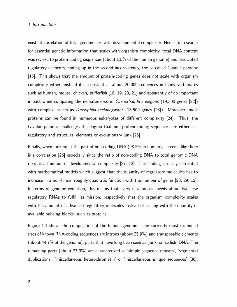
Figure 1.1 shows the composition of the human genome. The currently most examined
sites of known RNA-coding sequences are introns (about 25.9%) and transposable elements
(about 44.7% of the genome); parts that have long been seen as ’junk’ or ’selfish’ DNA. The
remaining parts (about 27.9%) are characterized as ’simple sequence repeats’, ’segmental
duplications’, ’miscellaneous heterochromatin’ or ’miscellaneous unique sequences’ [30].
2

Importance of RNA
Figure 1.1: The composition of the human genome. Only 1.5% are protein-coding se-
quences, 25.9% are introns. 44.7% of human DNA are transposable elements (long inter-
spersed nuclear elements (LINEs), short interspersed nuclear elements (SINES), long ter-
minal repeat (LTR) transposons and DNA transposons). Figure reproduced from Gregory
2005 [30].
However, latest research of the ENCODE pilot project in 2007 [31] estimates that about
98% of the chromosome are transcribed. More precisely, roughly 1% of the human genome
(chosen manually and by random in equal parts) was analyzed. We are far away from
answering the rising questions of the particular functions of these transcripts, in fact it is
even impossible to estimate whether all of these transcripts are functional or not, but the
findings challenge the idea of the genome being mainly an evolutionary junkyard. Instead,
it is more likely that self-splicing introns and transposable elements initiated a new level of
molecular evolution by expanding the pool of regulatory molecules in eukaryotic cells [12].
3

1 Introduction
Functions of RNA
The diversity of RNA sequences, sizes, structures and functions strongly suggests that we
have seen only a small fraction of all functional RNAs [32]. A comprehensive review about
known RNA functions would go far beyond the scope of this thesis, as RNA is involved
in virtually all levels of gene and cell cycle regulation [32, 33, 34]. I will therefore provide
a minimal outline of the most reviewed types of RNA, starting with classical RNAs that
are involved in protein synthesis and going on with an overview of (recently) characterized
ncRNAs.
The three major components of protein synthesis are ribosomal RNA (rRNA) that acts
as an catalyst and a big coordination apparatus, messenger RNA (mRNA) that serves as
coding-template and transfer RNA (tRNA) that decodes the mRNA via the delivery of
certain amino acids for the emerging protein. Whereas rRNA and tRNA are merely tran-
scribed and fold into their functional conformation spontaneously, mRNA is post-processed
in eukaryotic cells, involving small nuclear RNA (snRNA) [35] to splice non-protein-coding
parts (introns) out of the primary mRNA transcript. Some of these snRNAs are also re-
ported to be involved in transcription initiation by RNA polymerase II [36] and probably in
cell cycle regulation [37].
The family of small nucleolar RNAs (snoRNAs) [38] is known for the modification of other
RNAs. Their length varies between 60 and 300 nucleotides, where the functional part is
mainly concentrated to small regions (so-called boxes of about 18 nucleotides) that were
shown to interact with rRNAs, snRNAs and mRNAs. Beyond that there are various orphan
snoRNAs that cannot be associated with any target so far [34, 38]. This kind of RNA is
mainly reported to be transcribed from introns; some of them are involved in tissue-specific,
developmental regulation, others are involved in genomic imprinting [39, 40]. The human
telomerase (hTR) enzyme needs an integral RNA subunit to provide a template for the
4

Importance of RNA
replication of chromosome ends. Interestingly, this RNA subunit contains the same box we
know from snoRNAs, necessary for hTR accumulation and stability [38].
Micro RNAs (miRNAs) and short interfering RNAs (siRNAs) appear to be an important
component of translational repression. Both are between 21 and 25 nucleotides long and
influence gene expression by binding their targets via almost complementary base-pairing
to suppress gene expression, or a perfect complement to trigger degradation with the RNA
induced silencing complex (RISC) [41, 42], a process that is known as RNA interference
(RNAi) [43]. The differentiation between miRNA and siRNA becomes indistinct as more
and more research is done, but there are differences in their biogenesis. While miRNAs are
derived from endogenous DNA (introns and exons of coding and non-coding transcripts),
siRNAs are derived from less conserved endogenous and exogenous sources (transposons
and dsRNA viruses). Nevertheless, both are finally processed by an endonuclease that
cuts different kinds of precursor RNAs into small imperfect duplexes with a 2 nucleotide
overhang on their 3’ ends [44, 45]. So far they have been found to be associated with
developmental timing, cell proliferation, left-right patterning, neuronal cell fate, apoptosis
and fat metabolism in model organisms [44, 46, 47, 48], as well as neuronal gene expres-
sion [49], brain morphogenesis [50], muscle differentiation [51], stem cell division [52] and
chromatin regulation [53].
Another upcoming field of interest are long ncRNAs with an estimated size from 200
to 10.000 nucleotides [54]. These RNAs are involved in chromatin modification [55, 56],
transcriptional regulation [57, 58, 59] and post-transcriptional regulation [60, 56]. As their
overall sequence conservation is very low, long ncRNAs are hard to find by comparative
genomics.
In addition to these very well studied examples, the Piwi-interacting RNA (piRNA) is
involved in the protection of the germline genome by silencing endogenous repetitive se-
5

1 Introduction
quences and transposons [61]. The most recently described quelling defective/deficient
RNA (qiRNA) may inhibit protein synthesis on DNA damage checkpoints [62, 63].
Taking into account that this brief introduction into RNA is far from complete and that
new RNA representatives are reported continuously, it is not a big surprise that more and
more diseases are shown to be interrelated with regulatory RNA. A few examples are RNAs
that have been linked with neurobehavioral and developmental disorders and various forms
of cancer [64, 65, 66, 67, 68, 69, 70].
1.2 RNA world hypothesis
A basic question that remains unclear when discussing the origins of life is the evolution of
DNA, RNA and proteins. DNA is known as the genetic information storage, but does not
have enzymatic activity itself. Protein synthesis requires RNA as the template and within
the construction machinery. In a search for a common ancestor of life, we therefore end
up with the idea that it is either RNA or an other unknown precursor molecule. Indeed,
RNA can act as an auto-catalyst (ribozyme), as well as a catalyst for protein synthesis
(ribosome), it can store information, replicate itself and synthesize DNA. Moreover, many
co-substrates of protein enzymes contain ribonucleotides (ATP, NAD+, FAD, Acetyl-CoA).
This lead to the idea of an RNA world [71] that induced evolution out of the primordial
soup and paved the way to the first reproductive cell. However, the synthesis of the
first nucleotides without protecting groups and activation steps from the primordial soup
remained unreproducible for a long time and the survival of one spontaneously formed
RNA molecule is still hard to comprehend. A new approach for the synthesis of pyrimidine
ribonucleotides was recently published by Powner et al. [72]. The traditional strategy forms
ribose and the nucleobase separately from elements in the primadorial soup, but fails to
6

Synthetic biology
connect these parts to form a ribonucleotide. Powner et al. [72] found an alternative way to
form an activated pyrimidine ribonucleotide from plausible prebiotic feedstock molecules.
It remains unclear whether it is possible to generate self regulatory RNA molecules as a
next step to life from the primordial soup, but such promising research results suggest that
today’s life originated from spontaneously formed RNA molecules.
1.3 Synthetic biology
Traditional biological science tries to understand organic systems by the process of de-
scription, modification and re-description. While forward genetics identified changes in the
genotype by their effect on the phenotype (for instance by mutagens), the newer field of
reverse genetics modifies the genotype to see changes in the phenotype. Within the last
years, a third level of biological science is coming up: synthetic biology. The goal of this
emerging field is the departure from natural genomes that evolved for billions of years and
are so highly complex in their function that they may never be completely understood.
Instead, synthetic biology tries to (re-)assemble small minimal systems that fulfill predeter-
mined functions. With this constructive approach we may be able to design new biological
parts, devices and systems that do not exist in the natural world, as well as redesign existing
systems to perform specific tasks.
In the last ten years, within the first wave of synthetic biology [73], multiple simple artificial
components were developed, inspired by biological cells and electrical engineering. These
genetic tools include logical switches [74, 75, 76, 77, 78], logical gates [79, 80, 81, 82, 83, 84,
85], synthetic biosensors [86, 87], cell-cell communicators [88, 89] and oscillatory networks
[90, 91, 92, 93, 94, 95]. Combining these tools to somewhat more advanced units provides
a basis for memory management [96, 97], response to certain input thresholds [88, 98, 99]
and process-timing [100, 101]. There are also practical examples of modified cells for
7
1 Introduction
image processing [102, 103, 104], cells that can break up biofilms [105], invade cancer
cells [106], enhance antibiotic treatment [107] or produce an anti-malaria drug precursor
molecule [108]. Moreover there are multiple strategies to build artificial molecular motors
[109, 110, 111, 112, 113, 114, 115, 116], that may eventually provide a basis for a synthetic
cytoskeleton.
The goal of the second wave of synthetic biology should be the standardization of in-
put/output (I/O) devices that may be assembled to complex systems in a plug and play
fashion [73, 117].
An ambitious challenge is to establish a small system that is somehow capable of with-
standing or correcting mutations, can reproduce itself and therefore remains operational for
a longer period of time. Characteristics that are generally seen to be necessary for a ’living’
organism. Variations of such synthetic organisms can be utilized for eco-engineering, such
as hazardous waste disposal [118], production of bio-fuels [119] and drugs [120], as well as
to sense and fight cancer cells [106].
In order to construct a living system, one needs a chassis that separates the system from
the environment but permits permeation between both sides (the cell wall) and an internal
metabolism handling its reproduction. Such a functional metabolism that is geared to a
biological cell needs multiple components that interact with each other but do not harm
themselves by accidental interactions. Considering that the evaluation of each newly intro-
duced tool in such a system needs the inspection of targeted interactions and unintentional
cross-interactions on multiple levels (modified gene expression, affected RNA/protein func-
tion) the convergence to a new minimal organism is a combinatorial problem. There are
two approaches for the construction of living systems. The top-down approach to create a
minimal living cell tries to start from a small bacterial genome, such as Buchnera aphidicola
with an estimated size of 450kb and 400 genes [121], shrinking its genome by gene deletion
8

Riboswitches
as much as possible (to about 100-150 genes [122]). In contrast, the bottom-up approach
wants to build a model organism from scratch that is completely regulated by sophisticated
artificial components [123].
A basic necessity to establish a bottom-up system is the setup of artificial encapsulation and
controlled cell-division. The most promising building block candidates for encapsulation are
lipids, as they form dense, flexible bilayers and allow transformation in combination with
trans membrane proteins[124]. Approaches to set up minimal metabolic networks within
vesicles composed of different phospholipids can already be found in literature[124], but
controlled cell-division failed, as it needs the internal production of lipids, amino acids and
a functional cytoskeleton that defines the steric configuration within the cell, especially
during cell division itself. An autonomous semi-synthetic cell, handling DNA replication,
transcription, translation, cell growth and cell division should need approximately 100-150
genes [122, 125].
Coming from the RNA world hypothesis (see section 1.2, page 6), an even more minimal
replication system is based entirely on fatty acid vesicles that enclose a self replicating RNA
replicase [126]. The fatty acid vesicles are semipermeable for the uptake of nucleotides and
RNA replication leads to swelling of the vesicle, due to osmotic pressure. This swelling
results in the incorporation of new fatty acids, uncontrolled cell-division and a pH gradient
that could provide energy for the uptake of small molecules [127].
1.4 Riboswitches
The importance of RNA as a low-cost regulatory molecule in the cell has been discussed
in section 1.1. A particular form of both transcriptional and translational repression is
carried out by riboswitches. These RNA molecules, originally reported to be located in 5’-
9
1 Introduction
untranslated regions (5’-UTR) of bacterial mRNAs, are composed of an aptamer domain
that is responsive to small metabolites and a downstream functional expression platform
that can be in an ON or OFF state.
On translational level aptamer sequences of riboswitches fold into a stable conformation,
that either represses the function of the expression platform or not, the switch is in OFF or
ON state, respectively. A metabolite that attaches to the aptamer conformation rearranges
the configuration and thereby induces a turn-over of the switch from one state to the
other. Alternatively, theses aptamer regions can induce transcription termination, e.g. by
the formation of a stable hairpin that causes stalling of the ribosome and therefore the
release of an unfinished transcript [128].
The spectrum of known natural riboswitches is constantly expanded. Various aptamer do-
mains can sense purine nucleobases, amino acids, vitamin cofactors, amino-sugars, metal
ions and second messenger molecules [129]. Bacterial riboswitches regulating gene tran-
scription and translation are found in the 5’-UTR; eukaryotic riboswitches are reported in
introns or 3’-UTR of mRNA transcripts, involved in the regulation of splicing as well as
transcription regulation [130].
Of special interest for this thesis is an engineered RNA-triggered riboswitch presented by
Isaacs et al. [1] that is based on a cis-repressed RNA (crRNA) and a trans-activating
RNA (taRNA). After transcription, the ribosome binding site (RBS) forms a stable hairpin
structure with the aptamer domain, leading to a trapped (cis-repressed) OFF state. Tran-
scription of a taRNA does induce a conformational change that resolves cis repression and
induces gene translation; the switch is in an ON state (see figure 1.2). This minimal model
of translational control provides a potent basis to design a library of crRNA-taRNA couples
that regulate gene expression independently. In a synthetic cell, computationally optimized
taRNAs could trigger gene expression of multiple crRNAs, as well as start cascades of gene
10

Riboswitches
OFF intermediate ON
Figure 1.2: Synthetic RNA switch published by Isaacs et al. After transcription, the
riboswitch is in a cis-repressed OFF state (crRNA), as the ribosome binding site (RBS)
is not accessible and the therefore the transcription start side (AUG) is not functional.
Upon activation with a trans-activation RNA (taRNA), the two structures interact via an
Linear-loop complex conformation and finally refold to an RNA duplex structure that has
an accessible RBS. Image reproduced from [1].
networks in response to molecular clocks [101].
Our goal is to model the refolding kinetics of this riboswitch, in order to establish a frame-
work for the evaluation of new in silico designed riboswitches. The main challenge regards
the intermediate state of the refolding path. This Linear-loop complex (schematically shown
in figure 1.2) forms a structure motif that is comparatively rare and energetically hard to
evaluate. Most RNA structure prediction algorithms therefore exclude such motifs, as they
are predominantly interested in fast computation of frequent RNA structures. This inter-
mediate state, however, enables a fast rearrangement of the two RNA molecules and needs
to be considered for folding kinetics. In the following sections, we will therefore present
the program RNAscout.pl, which heuristically estimates a set of intermediate structures
(including the one shown in figure 1.2) that are expected to influence the refolding time.
Based on this network we will simulate the change of population probabilities of individual
structures and show that our results should be a good approximation of the natural behavior
of the riboswitch.
11
1 Introduction
Outlook
Within the following sections a detailed introduction of in silico RNA structure prediction
(section 2) will be provided, starting with nature and representations of RNA structures.
This will lead to a (historical) overview about general, conventional RNA folding algo-
rithms (mainly focusing on the recursions of the Vienna RNA package [2]), and a short
review about pseudoknot prediction and energetic evaluation of given pseudoknotted RNA
structures. On this basis we will discuss the energy model of RNAscout.pl, a program
to estimate folding kinetics of RNA-switches. Section 3 will explain current approaches to
calculate folding kinetics, mainly dealing with conventional RNA secondary structures and
the new heuristic approach of RNAscout.pl in RNA pseudoknot structure space. Finally
section 4 discusses results of RNAscout.pl compared to other existing programs, and sec-
tion 5 gives a short discussion and perspective towards the design of artificial RNA-triggered
RNA switches.
12

2 RNA structure prediction
From a chemical point of view ribonucleic acid (RNA) molecules are composed of three
different building blocks. Two of them, the phosphate group (PO−4 ) and the ribose (β-O-
2-ribofuranose) form the backbone of RNA molecules. The 5’ and 3’ carbons of the ribose
are bound to two oxygen atoms of the phosphate group, respectively; the 1’ carbon of the
ribose is connected to the third building block, the base.
There are four common types of RNA bases: Adenine (A), Guanine (G), Cytosine (C) and
Uracil (U) that can interact via hydrogen-bonds to stabilize the structure (see figure 2.1).
The dominating interaction motifs are the canonical base-pairs, which are the Watson-Crick
base-pairs (AU, UA, GC, CG) [131] and the wobble pairs (GU, UG) [132]. The importance
of these six base-pairs results from their isostericity, i. e. that the relative orientation of
the phosphate-ribose backbone is not dramatically affected upon reversal of the particular
base-pairs. Their dominance in RNA structure motifs makes these six base-pairs sufficient
for reliable RNA secondary structure prediction. Although many other kinds of non-isosteric
base-pair interactions are described in literature [133, 134], they have a comparatively low
occurrence in nature and are neglected in most applications to speed-up (enable) structure
prediction.
13

2 RNA structure prediction
O
OH
base
O
base
O
P
baseCH3
-
O
O
OO
P-
O
O
OO
OH
OH
OH
(a) RNA backbone
N
N
N
NN
H
H
N
N
O
O
H
Ribose
Ribose
Adenine (A) Uracil (U)
(b) A–U Watson-Crick base-pair
N
N
N
NO
N
N
N
N
O
H
H
H
H
H Ribose
Ribose
Guanine (G) Cytosine (C)
(c) G–C Watson-Crick base-pair
N
N
N
NO
NH2
N
N
O
OH
H
Ribose
Ribose
Guanine (G) Uracil (U)
(d) G–U wobble base-pair
Figure 2.1: The building blocks of RNA molecules. (a) The RNA backbone is formed
by phosphate groups (PO−4 ) and ribose (β-O-2-ribofuranose) molecules. Figures (b, c, d)
show the Watson-Crick base-pairs (A–U, G–C) and the wobble pair (G–U), respectively. The
individual bases form hydrogen bonds to interact; while A–U and G–U form two hydrogen
bonds, the G–C base-pair forms three of them. RNAs with a high G–C content are therefore
usually more stable than those with low G–C content.
14

Conventional RNA structure prediction
2.1 Conventional RNA structure prediction
2.1.1 RNA secondary structures
Analogous to proteins, there are three different types of structured levels for RNA. A
non-interacting ’open-chain’ molecule can simply be described by the succession of bases.
This primary structure (see figure 2.2a) particularly makes sense for previously mentioned
mRNAs that serve as templates for translation. However, as the primary structure does
not provide any information about the steric configuration, it is not descriptive in terms of
non-coding RNA function.
A more advanced representation of an RNA molecule is the secondary structure which il-
lustrates the base-pairing pattern but disregards the specific atomic positions in space (see
figure 2.2b). The profit of this representation is that it is possible to determine whether sin-
gle bases are paired or if they are accessible for molecular interactions (i. e. ribosome binding,
siRNA binding, . . . ). Moreover, secondary structure information serves as an indicator for
molecular function (e.g. ribozyme interaction motifs, tRNA structure conservation). The
RNA secondary structure representation is of importance for RNA folding algorithms, since
the formation of secondary structure motifs occurs much faster than tertiary interactions.
This characteristic is known as hierarchical folding in literature [135].
Finally, the tertiary structure depicts the actual configuration of the RNA molecule in
space (see figure 2.2c). A number of programs that predict tertiary structures based on
secondary structure prediction algorithms have recently been released (e. g. FARFAR [136],
iFoldRNA [137] and ModeRNA [138]). Predictions become better, however, reliable tertiary
structures can only be elucidated by experimental setups such as crystallography.
In terms of computational RNA biology, we define an RNA primary structure as a string
15

2 RNA structure prediction
GCCCGGAUGAUCCUCAGUGGUCUGGGGUGCAGGCUUCAAACCUGUAGCUGUCUAGCGACAGAGUGGUUCAAUUCCACCUUUCGGGCGCCA
(a) primary structure
GCCCGGA
UGA
U
CCUCAGUG
GU C U G G G G
UGCA
GGC
UUC A
AACCUGUA G C
UGUC
UAG
CGA
CA
GAG U G G
U UCAAUU
CCACCUUUCGGGCGC
CA
VLR
(b) secondary structure (c) tertiary structure
Figure 2.2: Three different kinds of structure representation of the human selenocysteine
tRNA [139] are shown. Usually tRNAs are composed of four stems and a variable loop region
(VLR). In this case the VLR forms a fifth hairpin structure. (a) The primary structure as
a string of nucleotides, (b) the secondary structure showing helices and loops in form of a
squiggle plot and (c) the complete tertiary structure. See figure 2.3 for different kinds of
secondary structure representations.
16
Conventional RNA structure prediction
S consisting of a finite alphabet∑
RNA = A, C, G, U, representing the four bases. The
secondary structure is a set Ω of base-pairs (i, j) along the sequence of length n [x1, . . . , xn],
which is defined by four rules.
1. If (i, j), (i, k) ∈ Ω then j = k
2. If (i, j) ∈ Ω then j − i > 3
3. If (i, j), (k, l) ∈ Ω and i < k then i < k < l < j or i < j < k < l
4. If (i, j) ∈ Ω then (xi, xj) ∈ BAU, UA, GC, CG, GU, UG
Rule 1 states that a base cannot form more than one base-pair. Rule 2 defines a minimum
hairpin loop size of three bases. Rule 3 states that all base pairs are nested or independent
of each other. Rule 4 defines the set of canonical (isosteric) base-pairs that are allowed for
standard RNA structure prediction.
Each of these rules restricts the conformation space of in silico predictable RNA secondary
structures to a biologically relevant and computationally tractable subset of possible con-
formations. However, increasing attention is paid to the fractional amount of non-nested
structural elements, so called pseudoknots that violate rule number 3 and rare structural
subsets that violate rules 1 and 4. Therefore, advanced RNA pseudoknot prediction algo-
rithms focus on these problems, with the drawback that they tend to compute pseudoknots
in known pseudoknot-free structure representations.
2.1.2 RNA structure representation
Graph representations
Conventional RNA secondary structures that are restricted by the rules from section 2.1.1,
can be depicted as planar graphs, i. e. graphs that can be drawn without crossing edges.
17
2 RNA structure prediction
Note that the reverse is not true, as some violations of the mentioned rules are still resulting
in planar RNA secondary structures. The squiggle plot, arc plot and circular plot are three
common layouts for certain kinds of planar RNA secondary structure representations.
Squiggle Plot The RNA backbone of an RNA molecule is drawn as a curved line and the
formed base-pairs are straight (usually short) lines connecting the particular bases. This
representation is very intuitive for small RNA structures, but becomes confusing rapidly
with increasing sequence length. One advantage of the squiggle plot is the capability to
represent all kinds of planar graphs. See figure 2.2b for an example of a squiggle plot.
Arc Plot / Book Embedding Arc plots consist of a straight line representing the RNA
backbone from 5’ to 3’ end. Base-pairs are represented by arcs connecting the bases. A
structure that follows the rules from section 2.1.1 can be shown on one side without arcs
crossing each other (see figure 2.3a). To depict pseudoknot interactions this representation
can be expanded to the book embedding representation. The RNA backbone is then seen
as the spine and each set of non-crossing base-pairs as a new page of the book. Pseudoknot
structures that can be shown with two pages of book embedding (see figure 2.6b) are also
called bi-secondary structures [140].
Circle Plot The succession of bases is drawn on a circle, with the 5’ and 3’ end next
to each other. Base-pairs are illustrated as straight lines that connect the particular bases
within the circle. A conventional secondary structure does not have any lines crossing each
other (see figure 2.3b), i. e. it is outerplanar. This representation is most restrictive, as a
pseudoknot interaction results in a non-outerplanar circle plot.
18

Conventional RNA structure prediction
Other representations
There are various other non-graph representations for RNA molecules. Three common
layouts are the dot-bracket string, mountain plot and the dot plot.
Dot-bracket string This string notation is the standard input and output of the Vienna
RNA package [2]. The alphabet of a secondary structure Ω is∑
Ω = (, ), ., with dots
representing unpaired bases and opening and closing brackets for a base-pairing upstream
and downstream. A secondary structure following the rules on page 17 can always be
represented by a well-formed bracket term. For structures including pseudoknots one needs
to introduce new parenthesis or a second dot-bracket string. See figure 2.3c for the classical
dot-bracket notation.
Mountain plot The RNA sequence is shown as a straight line. A base-pair towards the
3’ end is indicated as a uphill line, whereas a base-pair towards the 5’ end is shown by a
downhill line. Unpaired bases result in a horizontal line (see figure 2.3d).
Dot plot A base-pair (i, j) is shown as a dot in a matrix. Indices of rows and columns
correspond to the index of the sequence. The Vienna RNA dot plots show the minimum free
energy base-pairs within the left lower triangle of a matrix, the base-pairing probability is
shown in the upper right triangle, whereas the size of the dots proportional to the probability
of the base-pair.
19

2 RNA structure prediction
(a) Arc Plot (b) Circle Plot
GCCCGGAUGAUCCUCAGUGGUCUGGGGUGCAGGCUUCAAACCUGUAGCUGUCUAGCGACAGAGUGGUUCAAUUCCACCUUUCGGGCGCCA
(((((((.(..((((((....))))))((((((.......))))))((((((....))))))((((.......))))).)))))))....
(c) Dot-bracket string
GCCCGGAUGAUCCUCAGUGGUCUGGGGUGCAGGCUUCAAACCUGUAGCUGUCUAGCGACAGAGUGGUUCAAUUCCACCUUUCGGGCGCCA
(d) Mountain plot
G C C C G G A U G A U C C U C A G U G G U C U G G G G U G C A G G C U U C A A A C C U G U A G C U G U C U A G C G A C A G A G U G G U U C A A U U C C A C C U U U C G G G C G C C A
G C C C G G A U G A U C C U C A G U G G U C U G G G G U G C A G G C U U C A A A C C U G U A G C U G U C U A G C G A C A G A G U G G U U C A A U U C C A C C U U U C G G G C G C C AGC
CC
GG
AU
GA
UC
CU
CA
GU
GG
UC
UG
GG
GU
GC
AG
GC
UU
CA
AA
CC
UG
UA
GC
UG
UC
UA
GC
GA
CA
GA
GU
GG
UU
CA
AU
UC
CA
CC
UU
UC
GG
GC
GC
CA
GC
CC
GG
AU
GA
UC
CU
CA
GU
GG
UC
UG
GG
GU
GC
AG
GC
UU
CA
AA
CC
UG
UA
GC
UG
UC
UA
GC
GA
CA
GA
GU
GG
UU
CA
AU
UC
CA
CC
UU
UC
GG
GC
GC
CA
(e) Dot plot
Figure 2.3: Caption on page 21
20
Conventional RNA structure prediction
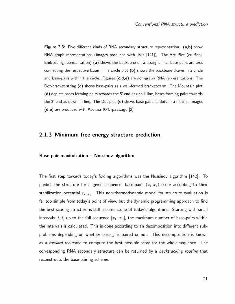
Figure 2.3: Five different kinds of RNA secondary structure representation. (a,b) show
RNA graph representations (images produced with JViz [141]). The Arc Plot (or Book
Embedding representation) (a) shows the backbone on a straight line, base-pairs are arcs
connecting the respective bases. The circle plot (b) shows the backbone drawn in a circle
and base-pairs within the circle. Figures (c,d,e) are non-graph RNA representations. The
Dot-bracket string (c) shows base-pairs as a well-formed bracket-term. The Mountain plot
(d) depicts bases forming pairs towards the 5’ end as uphill line, bases forming pairs towards
the 3’ end as downhill line. The Dot plot (e) shows base-pairs as dots in a matrix. Images
(d,e) are produced with Vienna RNA package [2]
2.1.3 Minimum free energy structure prediction
Base-pair maximization – Nussinov algorithm
The first step towards today’s folding algorithms was the Nussinov algorithm [142]. To
predict the structure for a given sequence, base-pairs (xi, xj) score according to their
stabilization potential ǫxi,xj. This non-thermodynamic model for structure evaluation is
far too simple from today’s point of view, but the dynamic programming approach to find
the best-scoring structure is still a cornerstone of today’s algorithms. Starting with small
intervals [i, j] up to the full sequence [x1..xn], the maximum number of base-pairs within
the intervals is calculated. This is done according to an decomposition into different sub-
problems depending on whether base j is paired or not. This decomposition is known
as a forward recursion to compute the best possible score for the whole sequence. The
corresponding RNA secondary structure can be returned by a backtracking routine that
reconstructs the base-pairing scheme.
21
2 RNA structure prediction
Advanced energy models
Today’s energy models do not focus on simple maximization of base-pairs, but utilize either
experimentally determined energy parameters (in combination with models from polymer
theory) or stochastic context-free grammars (SCFG) for probabilistic RNA modeling. An
example for the latter is CONTRAfold [143]. Its RNA structure prediction method is based
on conditional log-linear models, which generalize upon SCFGs by using discriminative
training with typical thermodynamical models [143].
Experimentally determined energy parameters are for example provided by the SantaLu-
cia [144] and Turner [145, 146] laboratories. Algorithms using these parameters uniquely
decompose structures into different kinds of loops(see figure 2.4). The total free energy of
an RNA secondary structure E(Ω) is then the sum of the free energies of its loops E(L).
E(Ω) =∑
L∈Ω
E(L)
A loop can be described by its length, i. e. the number of unpaired bases, and the degree k,
which is the number of closing base-pairs. Loops of degree k = 1 are called hairpin loops.
They have exactly one base-pair (i, j) that closes the loop. Loops of degree k = 2 are
either bulge loops (one unpaired strand), interior loops (two unpaired strands) or stacked
pairs (no unpaired base between two base-pairs). Stacked pairs are the basic modules to
build helices and stabilize structures. Finally, there are multi loops that have degree k > 2,
and so-called exterior loops, i. e. stretches of unpaired nucleotides which are not enclosed
by any base-pair. Figure 2.4 depicts all different kinds of loops.
The energy contribution of stacked pairs, small hairpins, certain interior loops and bulges
are experimentally measured [148, 146] and included into secondary structure prediction
programs using energy tables. Additionally, interaction penalties are provided for the for-
mation of intermolecular base-pairs.
22

Conventional RNA structure prediction
-
- -
-
-
--
-
-
Figure 2.4: Different types of loops. Interior base-bairs and closing base-pairs separate the
different loops towards the 3’/5’ end of the structure and the internal part of the structure,
respectively. The degree of a loop is dependent on the amount of interior and closing base-
pairs. Hairpin loops have degree 1, interior loops, bulges and stacking pairs have degree 2,
multi loops have a degree greater than 2. Image adapted from Flamm et al. [147]
The energy contribution of a loop is dependent on its length l (the number of unpaired
bases) and the type of the closing base-pair (i, j). Large hairpin loops H(i,j,l) where (l > x)
are extrapolated logarithmically by H(i,j,l) = H(i,j,x) + r ∗ log(l/x), where r is a constant
and x is set to 30 as default value in the Vienna RNA package. To keep the asymptotic
time complexity of algorithms in O(n3) where n is the length of the sequence, the length of
interior loops needs to be restricted. In case of the Vienna RNA package, the distance of
the two closing base-pairs (i, j); (p, q) is bound by a constant c such that p− i+ j− q ≤ c.
A multi loop energy M is composed of the cost for the formation of its closing-pair (a),
the energy contribution of each branch (b) and the destabilizing energy of every unpaired
base (c). This results in the following linear ansatz:
M = a + b ∗ k + c ∗ l (2.1)
where k is the loop degree and l is the sum of unpaired bases (i. e. the loop size).
23
2 RNA structure prediction
Zuker & Stiegler
Zuker & Stiegler were the first who came up with an algorithm to compute the MFE
secondary structure by loop-decomposition [149]. In principle they use the same dynamic
programming approach as in Ruth Nussinov’s base-pair maximization, except that new
terms for the type of a base-pair (i, j) are introduced. The energy contributions of a base-
pair includes hairpin loop energies H(i,j), interior loop energies (including bulges and stacked
pairs) I(i,j;p,q) and multi loop energies, which were originally considered as combinations of
interior loops and hairpin loops.
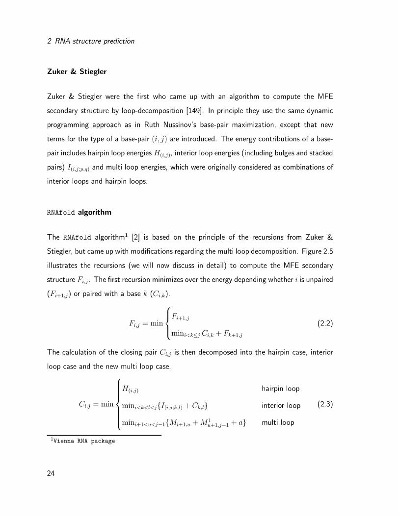
RNAfold algorithm
The RNAfold algorithm1 [2] is based on the principle of the recursions from Zuker &
Stiegler, but came up with modifications regarding the multi loop decomposition. Figure 2.5
illustrates the recursions (we will now discuss in detail) to compute the MFE secondary
structure Fi,j. The first recursion minimizes over the energy depending whether i is unpaired
(Fi+1,j) or paired with a base k (Ci,k).
Fi,j = min
Fi+1,j
mini<k≤j Ci,k + Fk+1,j
(2.2)
The calculation of the closing pair Ci,j is then decomposed into the hairpin case, interior
loop case and the new multi loop case.
Ci,j = min
H(i,j) hairpin loop
mini<k<l<jI(i,j;k,l) + Ck,l interior loop
mini+1<u<j−1Mi+1,u + M1u+1,j−1 + a multi loop
(2.3)
1Vienna RNA package
24

Conventional RNA structure prediction
The multi loop decomposition differs from the former algorithm of Zuker & Stiegler, as
it introduces a new term for the rightmost branch of the multi loop M1u+1,j−1, a term
containing the rest of the multi loop Mi+1,u and a, which is the penalty for a multi loop
initiation (see equation 2.1).
To have unique terms for multi loop decomposition, M1i,j can only contain the rightmost
stem of a multi loop and possible unpaired bases between its rightmost base and the closing
base-pair. This assures that every secondary structure is only calculated once during the
forward recursion, enabling to calculate probabilities of certain conformations within the
structure ensemble (see section 2.1.4). Both terms M1i,j and Mi,j can then be uniquely
decomposed to:
Mi,j = min
mini<u<j(u − i + 1)c + Cu+1,j + b
mini<u<j Mi,u + Cu+1,j + b
Mi,j−1 + c
(2.4)
M1i,j = min
M1i,j−1 + c
Ci,j + b
(2.5)
where b and c correspond to the destabilizing penalties from equation 2.1.
The computation of the forward recursions returns the MFE in F1,n where n is the length of
the sequence; the corresponding secondary structure is then computed by the backward re-
cursion. During this recursion, the generation of energy values in the matrices F, C, M, M1
is traced back and the base-pairing scheme of the MFE RNA structure is returned. This
algorithm requires O(n2) memory as the matrices F and C are stored for the backtracking
routine and has a time complexity of O(n3) due to the size restriction of interior loops.
The algorithm of RNAcofold [2] is based on the same principle, but is able to fold two
concatenated sequences. If there are intermolecular base-pairs, a penalty is added to the
25

2 RNA structure prediction
= FCi+1 k+1 j
F Fiji j i k
(a) Recursion 2.2
= hairpin C
interior
i j i i k l j
Cj ui+1 u+1i j−1 j
M M1
(b) Recursion 2.3
=
j j j−1i u u+1
Cu u+1
Ci jii
M MMj
(c) Recursion 2.4
M1 M1
=i ij j−1j
Ci j
(d) Recursion 2.5
Figure 2.5: Recursions of the Vienna RNA package. Pictures (a-d) correspond to recur-
sions 2.2-2.5 The minimum free energy of the structure interval (i, j) is stored in F . C
stores energies for the case where a base-pair is formed, M and M1 are energy tables for
multi loop handling. Image adapted from Hofacker & Stadler 2008 [150]
overall MFE structure. This is important for our riboswitch example discussed in section 1.4,
as we need to evaluate the energy of the RNA duplex structure (see figure 1.2).
2.1.4 Suboptimal RNA secondary structures
Of fundamental importance in RNA structure prediction is to keep in mind that there is
a huge space of possible conformations. Hence, the predicted RNA structure for a given
26
Conventional RNA structure prediction
sequence is the MFE structure according to the chosen energy model (at a certain temper-
ature, in a certain environment). However, there is no certainty that a given RNA molecule
does fold into the MFE structure, in fact it might be trapped in a local energy minimum
until it is degraded. It is therefore advisable to regard all suboptimal conformations within
a defined energy range to see whether there are structurally distant conformations that
have comparable energies.
Zuker suboptimal folding
An early approach for the calculation of suboptimal structures was shown by Zuker [151].
The algorithm returns the energetically best structure for each possible base-pair which is
computed from the energy terms Cij + Cij. The term Cij contains the best structure on
the sub-sequence (i..j) given that i and j are paired, i. e. the MFE structure inside the
base-pair. Cij contains the best possible structure from (1..i) and (j..n), i. e. the MFE
structure outside the base-pair. For a sequence of length n, theoretically n2
2structures can
be returned. In practice an RNA molecule can form far less than n2 individual base-pairs,
due to the limitations resulting from the rules discussed in section 2.1.1. An advantage of
this set of suboptimal structures is that the amount of computed structures is comparatively
low. A drawback, however, is that some important suboptimal structures cannot be found.
Given the optimal sub-structures A and B and their suboptimal counterparts A′ and B′, a
probably energetically very good structure A′B′ cannot be found.
Wuchty suboptimal folding
Wuchty et al. [152] implemented the RNAsubopt2 algorithm, which is an approach to
compute the complete suboptimal folding space. The algorithm utilizes the same forward
2Vienna RNA package
27

2 RNA structure prediction
recursion discussed in the RNAfold section to track the minimum free energy of the given
RNA sequence. In contrast, the backward recursion is extended to produce more than
solely one (MFE) structure.
While the RNAfold algorithm searches for one best MFE structure ΩF with a depth first
search, RNAsubopt returns all structures Ωi that have a free energy such that: E(Ωi) ≤
E(ΩF ) + δ, where δ is the size of a user defined energy interval. RNAsubopt with δ = 0
returns all MFE structures, in contrast to RNAfold which will return only one of them.
The structural ensemble returned is called a complete set of RNA structures, i.e. it contains
the whole conformation space Q within the energy interval. Generating such a complete
structure set, one has to accept that the amount of produced structures increases expo-
nentially with the length of the sequence [153].
Stochastic sampling of suboptimal structures
An alternative to estimate an energetically wide structure space for long RNA sequences
is to use the stochastic backtracking option implemented in RNAsubopt. In this case,
the forward recursion additionally calculates the equilibrium partition function [154] and
chooses the conformation space Q representing structures according to their equilibrium
probability. The algorithm to compute the equilibrium partition function is similar to the
discussed RNAfold forward recursions. Instead of picking the minimum, the sum over all
possibilities is stored in the matrices. The former additions of loop energies are replaced
by the multiplication of Boltzmann weighted energies. The Boltzmann weight e−E(Ω)
RT is
computed with the energy of the secondary structure E(Ω), the gas constant R and the
absolute temperature T . The partition function Z sums over all Boltzmann weighted energy
28

RNA pseudoknot prediction
contributions.
Z =∑
Ω∈Q
e−E(Ω)
RT (2.6)
Based on Z the probability of a certain structure Ωi is equal to its Boltzmann weight divided
by the partition function:
P (Ωi) =e
−E(Ωi)
RT
Z(2.7)
The stochastic backtracking routine of RNAsubopt constitutes a secondary structure Ω with
the probability P (Ω). Therefore, the suboptimal structure output derived by stochastic
backtracking is not guaranteed to contain the MFE secondary structure, but it will contain
a statistically representative set of structures.
2.2 RNA pseudoknot prediction
We have seen that efficient dynamic programming algorithms for RNA folding require four
basic rules to define an RNA secondary structure (page 17). One of these rules ensures
that every formed base-pair dissects an RNA structure into two parts that cannot interact
any more. An RNA pseudoknot is known as a structural element that violates this rule
such that base-pairs are crossing. Formally, a secondary structure contains a pseudoknot if
there exist base-pairs (i, j), (k, l) ∈ Ω such that i < k < j < l.
2.2.1 RNA pseudoknot structures
Various kinds of crossing base-pairs result in pseudoknots of different complexity [140].
Some of them can be found in ribosomal RNA molecules [155], in the functional region
of Ribonuclease P [156, 157] or are known to be involved in eukaryotic self-cleaving in-
trons [158, 159]. In the viral kingdom, there are pseudoknotted self-cleaving RNA molecules
29

2 RNA structure prediction
ACCCAAAUCCAGGAGGUGAUUGGUAGUGGUGGUUAAUGAAAAUUAACUUACUACUACCAUAUAUCUCUAGA&GAAUUCUACCAUUCACCUCUUGGAUUUGGGUAUUAAAGAGGAGAAAGGUACCAUG
((((((((((.(((((((..(((((((((((((((((....)))))).)))))))))))..)))))))...&......[[[[.[[[.[[[[[[))))))))))....]]]]]].]]].]]]].....
(a) Dot-bracket including pseudoknots
(b) 2-page book embedding
Figure 2.6: Two forms of bi-secondary structure representation. The ampersand (&) de-
notes the interaction of two RNA molecules. The dot-bracket notation (a) depicts crossing
base-pairs with a second set of parenthesis, the book embedding representation (b) is ex-
tended with a second page to illustrate the pseudoknot. Both representations show the
most populated transition state during a kinetic simulation of the refolding riboswitch pub-
lished by Isaacs et al. [1]. The RNA molecule left of the ampersand is the trans-activation
RNA, the RNA molecule on the right side is the cis-repressed riboswitch. Figure 2.6b was
produced with JViz [141]
reported to be essential for replication, as well as for regulation of viral protein synthe-
sis [158].
In this thesis we will deal with a subset of pseudoknotted structures, so called bi-secondary
structures [140]. Every bi-secondary structure Ω is the union of two pseudoknot-free sec-
ondary structures Ωc + Ωpk. In terms of structure representation, the dot-bracket string
notation illustrates a pair (i, j) ∈ Ωc as ’(’ and ’)’ respectively, and a pair (p, q) ∈ Ωpk
as string ’[’ and ’]’. Book embedding shows (i, j) ∈ Ωc on the upper side, i. e. the first
page of the book and (p, q) ∈ Ωpk on the lower side, i. e. the second page of the book (see
figure 2.6). A bi-secondary structure excludes all kinds of nested pseudoknot structures.
30

RNA pseudoknot prediction
A very common bi-secondary structure is the H-type pseudoknot, where a hairpin loop
forms base-pairs with a single-stranded region outside of the hairpin. Both helices then
arrange such that they form one big helix structure together. These pseudoknots are found
frequently in various kinds of RNA classes [158], e. g. the human telomerase contains an
H-type pseudoknot that is essential for its catalytic function [160]. Another bi-secondary
pseudoknot motif is the interaction of two hairpin loops. This kissing-hairpin interaction
can result in a helix structure that is visually hardly distinguishable from a normal helix. A
very prominent example for such an interaction is the HIV Tar-Tar∗ complex [161].
The pseudoknot structure motif of interest for simulations of RNA-triggered riboswitches
is the linear-loop complex formation (schematically shown in figure 1.2). This initial in-
teraction subsequently leads to a pseudoknotted transition state (see figure 2.6) which, as
we will see in section 4.4, is temporary most populated during kinetic simulations. In the
equilibrium distribution, the two sequences are ending up in a pseudoknot-free RNA-duplex
formation (schematically shown in figure 1.2). Every intermediate conformation formed
during this (expected) refolding path is included within the set of bi-secondary structures.
The impact on refolding kinetics will be discussed in detail in section 3.2.
There exist various other defined sets of pseudoknot classes apart from bi-secondary struc-
tures. Following the book-embedding classification, the book-thickness (or page number)
can be used as classification of more complex, nested pseudoknots [140]. Alternatively,
Reeder & Gigerich define the set of predictable simple recursive pseudoknots [162] as those
where the involved helices do not contain any bulges and have maximum possible length.
A summary of pseudoknot classes traceable by different algorithms has been reviewed by
Condon et al. [163] and Reidys et al. [164].
31

2 RNA structure prediction
2.2.2 RNA pseudoknot folding
Pseudoknot folding algorithms include defined subsets of pseudoknots into RNA secondary
structure, since exhaustive pseudoknot prediction based on loop energies has been shown
to be NP-complete [165]. Some pseudoknot motifs are included in today’s energy mod-
els [166, 167], but considering the amount of possible conformations, a more general energy
model for pseudoknot structures would be highly desirable. A challenging aspect for the
evaluation of pseudoknot interactions is the necessity to include steric and topological con-
siderations. While the loop decomposition of standard RNA folding algorithms ensures that
every predicted structure is sterically possible, there is no such guarantee for pseudoknot
interactions. Instead, a predicted interaction of distant loops might be sterically impossible
due to the stiffness of separating helix regions. Furthermore, an RNA helix-turn requires
11 base-pairs; in order to exceed this length, a strand forming a pseudoknot would need
to wrap around the complementary strand. This is especially interesting when looking at
topological constraints of RNA hybridization kinetics, as pseudoknot interactions might
lead to a trapped, knotted intermediate structure [168, 169]. Taking such special cases
into account, published energy models for pseudoknot folding must be substantially more
complex than conventional loop-based energy models.
Heuristic approaches that do not guarantee to find the MFE secondary structure can include
a wide range of pseudoknot types. Kinefold [170] uses stochastic folding simulations at the
level of nucleation and dissociation of RNA helix regions, processes that have been shown
to be the time-limiting steps of RNA folding kinetics. A related algorithm (based on the
idea of iteratively forming stable stems) is implemented in HotKnots [171]. DotKnot [172]
uses dot plots generated by the Vienna RNA package as starting point for pseudoknot
construction. Alternative programs are based on genetic algorithms [173] or stochastic
context free grammars [174].
32
RNA pseudoknot prediction
Another promising approach from Cao & Chen deals with polymer physics, estimating loop
entropy and handling base-pair stacking as corresponding enthalpic term [175, 176]. Limited
experimentally measured loop entropy values restrict the set of predictable pseudoknots
mainly to H-type pseudoknots and a few other structural elements.
Dynamic programming approaches using loop-based energy models have been implemented
by Rivas & Eddy [177], Dirks & Pierce [178], Reeder & Gigerich [162], Beyer et al. [179] and
Reidys et al. [164]. The corresponding set of pseudoknot structures varies between certain
defined classes of H-type pseudoknots and certain examples of multiple nested pseudoknots.
2.2.3 Energy model of RNAscout.pl
To model the pseudoknot-like interaction of the RNA-triggered riboswitch published by
Isaacs et al. [1], we will stick to a very fast and simple energy model that can handle all
kinds of bi-secondary structures.
We have discussed that every bi-secondary structure Ω is the union of two pseudoknot-free
secondary structures Ωc+Ωpk. However, the decomposition of a bi-secondary structure into
two secondary structures is not unique, so the following rules are applied to each pseudoknot
structure. Additionally to Ω, Ωc and Ωpk we introduce the temporary terms Ωleft and Ωright
to extract the pseudoknotted part of the structure, such that the leftmost base-pair and
the corresponding non-crossing base-pairs are stored in Ωleft and the crossing base-pairs
in Ωright. Energy evaluation of Ωleft and Ωright determines whether the base-pairs in Ωleft
and Ωright correspond to Ωc and Ωpk or Ωpk and Ωc respectively.
1. If (i, j) ∈ Ω and no (k, l) ∈ Ω such that i < k < j < l, then (i, j) ∈ Ωc
2. If (i, j), (k, l) ∈ Ω such that i < k < j < l, then (i, j) ∈ Ωleft, (k, l) ∈ Ωright
3. If E(Ωright) < E(Ωleft) then
33

2 RNA structure prediction
• Ωc = Ωc ∪ Ωright
• Ωpk = Ωleft
else
• Ωc = Ωc ∪ Ωleft
• Ωpk = Ωright
This simple decomposition of pseudoknot structures identifies the number of pseudoknots,
but not necessarily stores all energetically worse helices in Ωpk. In case we have a helix
crossing scheme A, A′ and B′, B, where A′ and B′ denote the energetically worse helices,
A, B′ and A′, B are always evaluated together and contribute either to Ωc or Ωpk. This
inexactness needs to be considered when evaluating refolding paths that contain more than
one individual pseudoknot.
The structural parts Ωc and Ωpk are then energetically evaluated with the standard Vienna
RNA folding algorithms and a pseudoknot initiation penalty β is added n times, where n
corresponds to the amount of individual pseudoknots.
E(Ω) = E(Ωc) + E(Ωpk) + nβ (2.8)
β can either be set as a loop-type independent (constant) value or adjusted depending on
the type of loop interaction. Results in chapter 4 were produced using a initiation penalty
β independent of the type of loop interaction. Related penalties for β are e. g. the duplex
initiation energy of 4.1 kcal/mol [146], which is used for various RNA-RNA interaction
penalties in the Vienna RNA package, the penalty of DotKnot [172] of 7 kcal/mol, the
penalty of RNApkplex [179] of 8.1 kcal/mol or the even higher pseudoknot penalty of
pknotsRG [162] with 9 kcal/mol. The pseudoknot interaction penalty of RNApkplex was
shown to be most accurate in combination with the energy model of the Vienna RNA
package [179], therefore it is used as the default β for our evaluation of pseudoknot
34

RNA pseudoknot prediction
structures. Note, that if we are dealing with the modeling of the pseudoknot-like interaction
between two different sequences, two penalties are added for the initial crossing base-pair.
The pseudoknot penalty of 8.1 kcal/mol and the duplex initiation penalty of 4.1 kcal/mol
for the initial interaction between two sequences.
35
3 Folding kinetics of RNA structures
RNA molecules are dynamic polymer chains that constantly rearrange within their environ-
ment, in order to minimize their free energy. In the following, we will focus on (re-)folding
kinetics of RNA structures. In particular, the goal is to estimate the time a given RNA
starting structure Ωi needs to refold into an energetically better structure Ωj . We will start
this chapter with the definition of a folding landscape, which is the basis for subsequent
calculations. The following sections will then discuss approaches to calculate folding ki-
netics within small exhaustively computable landscapes and large heuristically estimated
landscapes.
A folding landscape is defined as a triple (Q, M , E).
• The conformation space Q
⇒ defines the set of possible conformations
• The move-set M
⇒ defines the set of possible transitions and thus dictates a neighborhood/metric
within Q
• The energy (or fitness) function E
⇒ A relation that assigns a real value to each conformation, defining the shape of
the landscape
36

RNA Conformation Space (Q)
The conformation space Q of an RNA molecule can be divided into different sections of
biological relevance. The minimum free energy structure ΩF is considered as the most
relevant part, followed by a set of suboptimal structures. The free energy of an open chain
molecule, i. e. a completely unpaired secondary structure, is 0 kcal/mol by definition and
dissects the part of relevant (suboptimal) structures from the part of irrelevant structures
whose conformation energies are greater than that of the open chain molecule (at the
given temperature). The amount of suboptimal structures grows exponentially with the
length of an RNA molecule, such that exhaustively enumerating all suboptimal structures is
feasible for small RNA sequences only. Whereas most RNA secondary structure prediction
algorithms aim to compute the MFE secondary structure ΩF , it is advisable to consider
all RNA secondary structures within a certain energy range E(Ωi) ≤ E(ΩF ) + δ to see
whether there are structurally distant conformations with comparable free energies (see
section 2.1.4).
The type of conformation space (i. e. the set of structures that is included) can be of crucial
impact when searching for refolding paths. In the following we will distinguish between two
types of RNA conformation spaces:
• the conventional secondary structure space Qconv
• the bi-secondary pseudoknot structure space Qpk
Qconv covers all RNA secondary structures that can be predicted by conventional RNA
structure prediction; thus, it is bound by the rules on page 17. Qpk covers Qconv and all
bi-secondary pseudoknot structures (see section 2.2). Considering that Qpk is a superset
of Qconv, the amount of structures included within the same energy range is far higher in
Qpk than in Qconv.
37

3 Folding kinetics of RNA structures
Figure 3.1: This elementary move-set for RNA structures includes only the insertion or
deletion of a single valid base-pair.
The move-set (M)
The move-set M describes a notion of neighborhood and defines a metric within the
conformation space Q. Hence, it must fulfill the following properties:
1. Reversibility: Every move has an inverse counterpart, there are no one-way moves
that may lead to a trapped structure.
2. Validity: Every move results in a valid (neighboring) structure.
3. Ergodicity: Every structure Ωi is reachable from every other structure Ωj within Q.
The most elementary move-set one can think of for RNA structures is the insertion or
deletion of a single valid base-pair (see figure 3.1).
The combination of conformation space and move-set allows to detect paths (Πj⇐i) be-
tween two RNA structures Ωi and Ωj . A path Πj⇐i is obtained by iterative moves to
38

neighboring structures until a starting structure Ωi is completely transformed into Ωj .
The energy function E
The energy function E assigns energies to each conformation within Q. Typical energy
models to score conventional RNA structures and RNA pseudoknot structures have been
discussed in section 2.1 and section 2.2, respectively. The energy function determines the
shape of an energy landscape, enabling to calculate whether a move (or transition) between
neighboring structures is likely or not. The computation of transition probabilities will be
discussed in detail in section 3.1.2.
Characterization of energy landscapes
Having discussed the general definition of folding landscapes, we are now interested in
the characteristics of particular landscapes. Importantly, we would like to have parameters
describing whether RNA structures can fold efficiently into their MFE secondary structure
or might be trapped in local minimum conformations.
A theoretical parameter is the so-called ruggedness of an energy landscape. One way ap-
proach quantify the ruggedness is to compute the amount of local minima of an energy
landscape [180]. Formally, for every local minimum structure Ωi and all of its neighboring
structures Ωi′ it holds that E(Ωi) ≤ E(Ωi′). Coming from simulated annealing, another
approach is to measure the depth of an energy landscape. The depth describes the max-
imum height of barrier energies separating the local minima. In the theory of simulated
annealing, depth and the correlated difficulty of an energy landscape determine how fast
the global optimum of an energy landscape can be found from arbitrary starting confor-
mations [181]. A saddle point (or barrier structure) Bji that separates two different local
39

3 Folding kinetics of RNA structures
minima Ωi and Ωj is the energetically worst structure on the energetically best path Πj⇐i
within the set of all paths Pj⇐i (see figure 3.2).
E(Bji) = minΠj⇐i∈Pj⇐i
maxΩ∈Πj⇐i
E(Ω) (3.1)
The barrier height (H) on a path Πj⇐i can be calculated by the energy of the transition
state E(Bji) and the energy of the starting minimum E(Ωi):
Hji = E(Bji) − E(Ωi) (3.2)
Coming back to our goal to calculate (re-)folding kinetics between two RNA structures Ωi
and Ωj , we need to compute a set of suboptimal structures, such that at least one path
Πj⇐i connecting the structures can be found. The transition probability from Ωi to Ωj is
then dependent on the energy barrier separating the two structures.
In our example of the structural rearrangement of the taRNA-crRNA couple published by
Isaacs et al. (see figure 1.2), we need to find the energetically best path from the starting
conformation ΩS (two independently folded MFE conformations) to the MFE conformation
ΩF (MFE RNA duplex conformation), considering that pseudoknot transition states might
shorten the best path possible within Qconv. The following sections will discuss a proper
way to calculate folding kinetics in a landscape based on a complete Qconv and approximate
approaches for calculations in a landscape based on a heuristic estimation of Qpk (Qpk).
40

Complete conformation space
Bji
E
iΩ
jΩ
Figure 3.2: Two basins of attraction of an RNA energy landscape, their associated local
minima Ωi and Ωj and the barrier structure (saddle point) Bji separating them.
3.1 Complete conformation space
3.1.1 ’barriers’ – characterization of folding landscapes
Computation of a barrier tree
The program barriers1 [182] computes all local minimum structures and separating barrier
conformations within a certain energy range by use of a flooding algorithm. An energetically
sorted list of Qconv (produced by RNAsubopt) is processed starting with the MFE structure.
The chosen move-set (i. e. base-pair moves) is applied to every conformation in the list
generating all possible neighbors. The resulting neighborhood is utilized to classify the
structures according to different cases:
1part of the Vienna RNA package
41
3 Folding kinetics of RNA structures
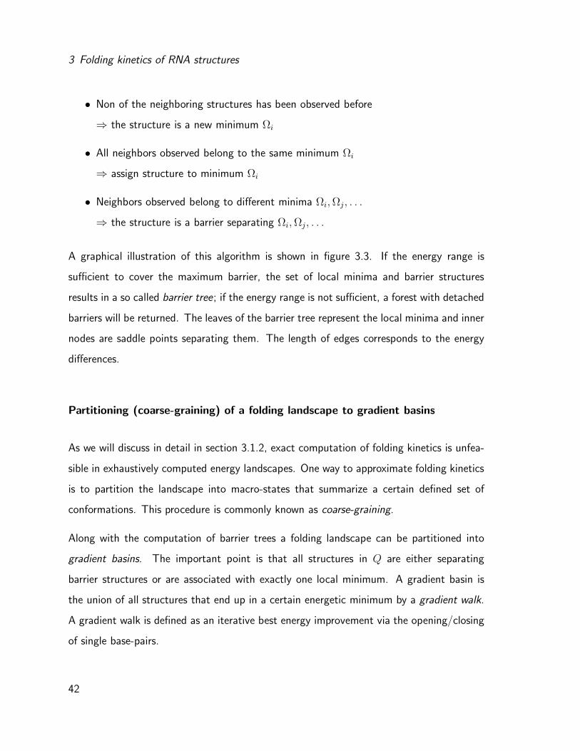
• Non of the neighboring structures has been observed before
⇒ the structure is a new minimum Ωi
• All neighbors observed belong to the same minimum Ωi
⇒ assign structure to minimum Ωi
• Neighbors observed belong to different minima Ωi, Ωj, . . .
⇒ the structure is a barrier separating Ωi, Ωj, . . .
A graphical illustration of this algorithm is shown in figure 3.3. If the energy range is
sufficient to cover the maximum barrier, the set of local minima and barrier structures
results in a so called barrier tree; if the energy range is not sufficient, a forest with detached
barriers will be returned. The leaves of the barrier tree represent the local minima and inner
nodes are saddle points separating them. The length of edges corresponds to the energy
differences.
Partitioning (coarse-graining) of a folding landscape to gradient basins
As we will discuss in detail in section 3.1.2, exact computation of folding kinetics is unfea-
sible in exhaustively computed energy landscapes. One way to approximate folding kinetics
is to partition the landscape into macro-states that summarize a certain defined set of
conformations. This procedure is commonly known as coarse-graining.
Along with the computation of barrier trees a folding landscape can be partitioned into
gradient basins. The important point is that all structures in Q are either separating
barrier structures or are associated with exactly one local minimum. A gradient basin is
the union of all structures that end up in a certain energetic minimum by a gradient walk.
A gradient walk is defined as an iterative best energy improvement via the opening/closing
of single base-pairs.
42

Complete conformation space
j
E
Bji
Figure 3.3: A graphical illustration of the flooding algorithm to generate barrier trees
(implemented in the program package barriers). Starting from the MFE structure, an
energetically sorted list of RNA conformations is processed to find local minimum structures
Ω and barriers (saddle points) B.
43
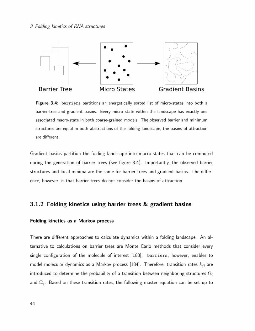
3 Folding kinetics of RNA structures
Barrier Tree Micro States Gradient Basins
Figure 3.4: barriers partitions an energetically sorted list of micro-states into both a
barrier-tree and gradient basins. Every micro state within the landscape has exactly one
associated macro-state in both coarse-grained models. The observed barrier and minimum
structures are equal in both abstractions of the folding landscape, the basins of attraction
are different.
Gradient basins partition the folding landscape into macro-states that can be computed
during the generation of barrier trees (see figure 3.4). Importantly, the observed barrier
structures and local minima are the same for barrier trees and gradient basins. The differ-
ence, however, is that barrier trees do not consider the basins of attraction.
3.1.2 Folding kinetics using barrier trees & gradient basins
Folding kinetics as a Markov process
There are different approaches to calculate dynamics within a folding landscape. An al-
ternative to calculations on barrier trees are Monte Carlo methods that consider every
single configuration of the molecule of interest [183]. barriers, however, enables to
model molecular dynamics as a Markov process [184]. Therefore, transition rates kji are
introduced to determine the probability of a transition between neighboring structures Ωi
and Ωj . Based on these transition rates, the following master equation can be set up to
44

Complete conformation space
determine the time-dependent probability of a structure Ωi.
dPt(Ωi)
dt=
∑
j 6=i
[Pt(Ωj)kij − Pt(Ωi)kji] (3.3)
The change in population density of a certain structure Ωi is calculated from the sum over
all incoming rates kij times the probability to be in Ωj minus the sum of all outgoing rates
kji times the probability to be in Ωi. The overall probability to end up in a certain structure
Ωi as a function of time can be obtained by explicit solution of the master equation.
A way to numerically solve this equation is to set up a rate matrix R that contains all
rates kij and the rates to remain in the current configuration, kii. Based on R, master
equation 3.3 can be rewritten in matrix form, which can be integrated numerically [185]:
d
dtPt = RPt (3.4)
The solution of equation 3.4 can then be calculated considering the initial and temporal
distribution vectors Pt and P0:
Pt = etRP0 (3.5)
where P0 is the population density at the time point t = 0. In order to solve equation 3.5, R
needs to be diagonalized. This is possible for a small rate matrix (with about 10000 states),
but unfeasible for a rate matrix including all states of a conformation space. barriers
therefore coarse-grains the folding landscape into gradient-basins (see section 3.1.1) and
returns a rate matrix R connecting these macro-states. The described equations to process
R are implemented in the treekin package2 [182]. The corresponding thesis [186] provides
a more detailed description of the mathematical background.
2Vienna RNA package
45

3 Folding kinetics of RNA structures
Modeling of transition rates
We have now found a way to numerically calculate folding kinetics on the basis of transition
rates. In principle there are several ways to compute rates between neighboring structures.
An important aspect that needs to be considered is detailed balance, i. e. ensuring that
microscopic fluxes between neighboring structures are reversible. In other words, the prob-
ability of being in structure Ωi (πi) times the rate towards Ωi from another state Ωj (kij)
needs to be the same as the probability of being in Ωj (πj) times the backward rate (kji):
πikij = πjkji (3.6)
On a grad scale, we need to ensure that the probability for a structure Ωj (πj) equals
the sum of over all rates towards Ωj (kji) times the probability to be in the respective
neighboring structure Ωi (πi).
πj =∑
i6=j
kjiπi (3.7)
barriers calculates rates between neighboring structures (i. e. transition rates) with the
Arrhenius Law. A transition rate kji is then calculated as:
kji = k0e−
E(Ωt)−E(Ωi)
RT (3.8)
where the transition state E(Ωt) is the maximum of E(Ωi) and E(Ωj) and k0 is a constant
to adjust the time dependency of a transition. k0 is set to 1 by default. Assuming that the
transition state is always the energetically worse state of the two neighboring conformations,
the Arrhenius law is the same as the Metropolis rule of simulated annealing, assuming that
a transition rate kji from structure Ωi to structure Ωj is always 1 if E(Ωi) ≥ E(Ωj), and a
small non-negative number calculated by the Boltzmann weighted distribution otherwise:
kji =
1 if E(Ωi) ≥ E(Ωj)
e−E(Ωj )−E(Ωi)
RT otherwise
(3.9)
46

Complete conformation space
The rate matrix R to solve equation 3.5 contains the rates calculated by the Arrhenius
Law kij and rates to remain in the current conformation kii. To ensure that the sum of
probabilities for each transition from a certain state (including the transition to remain in
the current conformation) is 1, the rates to remain in the current structure (the diagonal
of R) is calculated by the negative sum of all outgoing rates.
R(kij) =
kji if i 6= j
−∑
j 6=i kji if i = j
(3.10)
An exhaustive computation that considers rates between all possible conformations would
result in a huge size of R even for small sequences, making the solution of the master
equation unfeasible. As mentioned previously, it is necessary to coarse-grain the data set
into macro-states, for example by partitioning the landscape into gradient basins. The
open question is now, how to approximate rates between macro-states. If we assume that
the time spent in such a macro-state is long enough to reach the internal equilibrium, we
can compute rates between macro-states from the equilibrium probability of all structures
within a basin. This equilibrium probability within a basin α can then be computed by the
internal partition function Zα =∑
Ωi∈α e−E(Ωi)/RT . The probability of a structure Ωi in
the basin α is derived by dividing its Boltzmann weight by the partition function:
P [Ωi|α] =e
−E(Ωi)
RT
Zα
(3.11)
The rate connecting a basin α and β (rβα) is calculated from all individual rates rji, where
structure Ωi ∈ α and Ωj ∈ β:
rβα =∑
j∈β
∑
i∈α
rjiP [Ωi|α] for α 6= β (3.12)
When using the equilibrium partition function Z to compute rates between macro-states,
we approximate that it is of no impact which exact structure Ωi is picked within the gradient
47

3 Folding kinetics of RNA structures
basin. An exact computation would consider P [Ωi|α, t, Ωi0] with Ωi0 being the particular
state from which basin α was entered and t being the time dependency to reach state
i. With the assumption that the time is long enough to reach the equilibrium probability
independently from the starting state i0, the probability can be approximated as P [Ωi|α].
Note that rβα can be computed during the generation of barrier trees, as we are dealing
with a complete Qconv where every structure belongs to a certain basin of attraction. In the
following section (dealing with an heuristic Qpk), we need other approximations to calculate
transition rates.
3.2 Heuristically estimated conformation space
We have now discussed kinetics considering every possible conformation in the folding
landscape. However, the problem of finding the best energy barrier (Bij) separating two
RNA secondary structures in a conformation space (Q) that excludes pseudoknots was
shown to be NP-complete in 2010 [187]. In other words, exhaustive computation fails if
the energy barrier is too high and therefore the relevant part of the RNA conformation
space becomes computationally intractable. A number of algorithms that deal with path
finding heuristics to estimate barrier heights have been implemented and will be discussed
within this section.
If bi-secondary pseudoknot structures are included, the cardinality of Q increases to a
superset Qpk, making exhaustive computation unfeasible. However, sometimes there are
refolding paths that have a high energetic barrier in Qconv and a comparably low energy
barrier in Qpk (see figure 3.5). Section 3.2.2 will show an approach to estimate folding
kinetics from any starting structure ΩS into the MFE secondary structure ΩF .
48

Heuristically estimated conformation space
E
Q(conv)
Q(pk)
Figure 3.5: The RNA structure Ωi is a local minimum in the energy landscape. To refold
into conformation Ωj, the time consuming step is to pass the energy barrier (Bji). Bji
is the energetically worst structure on the best path Ωji. Within Qconv the barrier height
is far bigger than in the extended conformation space Qpk. Barrier heights were derived
from the findpath and pk findpath heuristic respectively, the complete best paths Ωj⇐i
within Qconv and Qpk can be seen in appendix A.1 and A.2.
49

3 Folding kinetics of RNA structures
3.2.1 Heuristic path generation
We have discussed previously that a transition rate and the corresponding probability of a
transition is proportional to the energy difference between two structures. In other words,
the height of the energy barrier along the best path Πj⇐i determines the transition rate.
The following heuristic algorithms have been implemented to determine the best path
Πj⇐i in large folding landscapes. In detail, they have been implemented for a conventional
conformation space Qconv and the elementary base-pair move-set (see page 38). Heuristic
approaches for path finding problems can be grouped into the general path heuristics and
the subset of direct path heuristics [188]. A direct path that transforms structure Ω1 into
structure Ω2 is generated by opening base pairs in Ω1 that are not contained in Ω2 and
introducing base-pairs from Ω2 that are not contained in Ω1. The length of a direct path is
therefore exactly the base-pair distance D(Ω1, Ω2) and the set of structures that is evaluated
for barrier estimation is excluding every structure with base-pairs (i, j) /∈ (Ω1 ∪ Ω2). The
evaluation of all direct paths is still too costly, but there are fast heuristics that estimate
barrier heights on direct paths. The Morgan & Higgs heuristic [188] performs a greedy
search with the following steps starting with Ω1:
• search for base-pairs exclusively in Ω2 that have the least number of incompatible
pairs in Ω1. Choose one randomly in case there are multiple base-pairs fulfilling this
condition.
• Remove the appropriate incompatible pairs from Ω1, add the new pair to Ω1 and, if
additional pairs can be formed, add these to Ω1.
• Repeat this procedure with the new intermediate structure until it is transformed into
the final structure Ω2.
Another fast and simple heuristic to generate direct paths between two structures is the
findpath routine [189]. findpath performs a breadth first search, generating all neighbors
50

Heuristically estimated conformation space
of the starting structure that are one step closer to the final structure and keeps the
energetically best m in memory. These candidates are then taken to produce the next best
m structures. To set an upper bound for barrier energies, findpath pre-computes a greedy
barrier energy with m = 1. During the subsequent breadth first search for direct paths,
those exceeding the upper bound are discarded.
Barrier heights derived from direct paths, however, are often worse than their indirect
counterparts. A statistical comparison of exact barrier heights and findpath barriers can
be seen in section 4.1, page 62. The performance of the heuristic decreases with growing
barrier heights. This observation is rather intuitive, as barrier heights are correlated with
the base-pair distance and therefore stabilizing base-pairs are increasingly relevant.
Morgan & Higgs [188] have therefore also presented a method to heuristically estimate
indirect paths. A set of low energy secondary structures is sampled and the starting and
end structures Ω1 and Ω2 are added. The resulting set of structures is seen as the vertices
of a graph. The corresponding edges are introduced by their greedy direct path heuristic
discussed above. By use of a single link cluster algorithm the optimal path from Ω1 to Ω2
within the network can be determined.
Another heuristic for the generation of indirect paths has been published by Dotu et al. [190].
Their algorithm detects indirect paths with a semi-greedy tabu search, storing a list of the
last k-visited conformations. Via iterative base-pair moves, structure Ω1 is transformed to
Ω2. One of the energetically best neighbors (not stored in the list of visited conformations)
is selected randomly and taken as the new transition state. The algorithm terminates if Ω1
is completely transformed to Ω2.
51

3 Folding kinetics of RNA structures
’pk findpath’ – direct paths in pseudoknot space
Even if both starting and end structures Ωi and Ωj are pseudoknot free, it is possible
that the intermediate conformations on a path Πj⇐i contain pseudoknots (see figure 3.5).
Especially, if there are conflicting helices that are able to form an energetically favorable
pseudoknot if they are partially formed. The principle of the pk findpath algorithm is a
breadth first search with a fixed upper bound analogous to findpath [189]. In contrast
to the previously described algorithm, pk findpath operates on an enhanced folding land-
scape. The conformation space is extended to a set of structures that includes bi-secondary
pseudoknot conformations (Qpk) and base-pair moves are extended to allow every kind of
crossing base-pair that results in a bi-secondary structure. The energy of conventional
secondary structures is evaluated by the standard loop based energy model described in
section 2.1.3; the energy of bi-secondary structures is computed by the extended energy-
function from equation 2.8.
A comparison of the predicted findpath and pk findpath barrier height for an RNA-
triggered riboswitch can be seen in figure 3.5. The complete refolding paths are shown in
appendix A.1 and appendix A.2. findpath predicts a pseudoknot-free refolding path with
a barrier structure Bji that has a free energy of -25.80 kcal/mol, whereas pk findpath
predicts a pseudoknot interaction resulting in a barrier structure with a free energy of
-32.30 kcal/mol. The corresponding barrier heights regarding the energy of the starting
conformation E(ΩS) = −42.40 kcal/mol are 16.6 kcal/mol and 10.1 kcal/mol, respectively.
A more general consequence of the altered landscape will be discussed in section 4.1. For
small barriers, findpath and pk findpath give the same results, as pseudoknot intermedi-
ate structures do not improve the barrier height. When comparing high barrier predictions,
we do see differences in the direct path generation as pseudoknots increasingly lower the
barrier energies.
52

Heuristically estimated conformation space
3.2.2 ’RNAscout.pl’ – heuristic folding landscapes
As an improvement to the previously described direct path heuristics, we will now try to esti-
mate indirect folding pathways with a small set of related neighboring conformations within
the conformation space Qpk. We will refer to this set of heuristically determined structures
as Qpk. The generated network of structures shall then be the basis to approximate folding
dynamics of the full conformation space Qpk.
In contrast to the ex ante generation of a complete Qconv by the backtracking procedure of
RNAsubopt, we will now discuss the generation of a partial Qpk starting from an arbitrary
starting structure ΩS and the MFE structure ΩF . The algorithm of RNAscout.pl builds
a recursive conformation graph, with vertices representing RNA secondary structures and
edges corresponding to the moves that generated the connected vertices.
RNAscout.pl utilizes a larger move-set than the previously introduced base-pair moves.
Structurally close conformations are lumped together into stacked, consecutive base-pairs
that are opened and closed in one step. Approximations of landscapes with such large move-
sets can cause problems in terms of ergodicity and reversibility (see section 3, page 38),
as certain thresholds lead to non-reversible steps during the graph construction. Thus,
transition rates between connected vertices are calculated in succession by use of the
pk findpath heuristic to ensure detailed balance within the generated heuristic landscape.
A conformation graph produced by RNAscout.pl allows two types of output evaluation.
The first possibility is to extract the minimum barrier from the generated network. In this
case, a path between any starting structures Ωi and Ωj can be evaluated for indirect barrier
detection. A comparison of predicted pk findpath barriers and RNAscout.pl barriers
can be seen in section 4.1. However, the single best path between two structures is not
sufficient to have a good approximation of the folding dynamics. Instead, we can calculate
folding kinetics within the whole generated network. In this case it is advisable to stick to
53
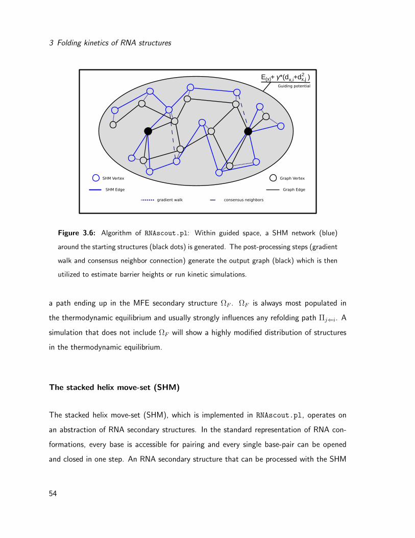
3 Folding kinetics of RNA structures
E + γ*(d +d )2x,jx,i(x)
Graph Edge
SHM Vertex
SHM Edge
Graph Vertex
gradient walk consensus neighbors
Guiding potential
Figure 3.6: Algorithm of RNAscout.pl: Within guided space, a SHM network (blue)
around the starting structures (black dots) is generated. The post-processing steps (gradient
walk and consensus neighbor connection) generate the output graph (black) which is then
utilized to estimate barrier heights or run kinetic simulations.
a path ending up in the MFE secondary structure ΩF . ΩF is always most populated in
the thermodynamic equilibrium and usually strongly influences any refolding path Πj⇐i. A
simulation that does not include ΩF will show a highly modified distribution of structures
in the thermodynamic equilibrium.
The stacked helix move-set (SHM)
The stacked helix move-set (SHM), which is implemented in RNAscout.pl, operates on
an abstraction of RNA secondary structures. In the standard representation of RNA con-
formations, every base is accessible for pairing and every single base-pair can be opened
and closed in one step. An RNA secondary structure that can be processed with the SHM
54
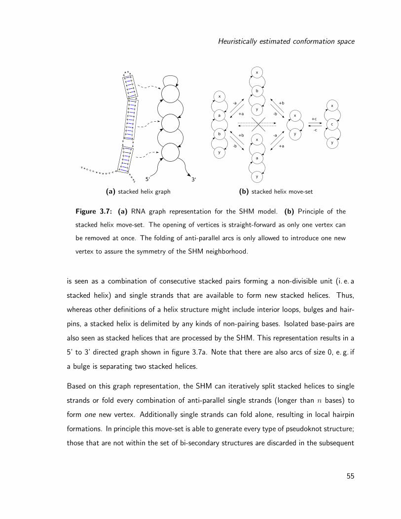
Heuristically estimated conformation space
3'5'
(a) stacked helix graph
x
y
a
b
y
x
b
y
x
a
y
x
y
x
c
-a
-b
-b
-a
+b
+b
+a
+a
+c
-c
(b) stacked helix move-set
Figure 3.7: (a) RNA graph representation for the SHM model. (b) Principle of the
stacked helix move-set. The opening of vertices is straight-forward as only one vertex can
be removed at once. The folding of anti-parallel arcs is only allowed to introduce one new
vertex to assure the symmetry of the SHM neighborhood.
is seen as a combination of consecutive stacked pairs forming a non-divisible unit (i. e. a
stacked helix) and single strands that are available to form new stacked helices. Thus,
whereas other definitions of a helix structure might include interior loops, bulges and hair-
pins, a stacked helix is delimited by any kinds of non-pairing bases. Isolated base-pairs are
also seen as stacked helices that are processed by the SHM. This representation results in a
5’ to 3’ directed graph shown in figure 3.7a. Note that there are also arcs of size 0, e. g. if
a bulge is separating two stacked helices.
Based on this graph representation, the SHM can iteratively split stacked helices to single
strands or fold every combination of anti-parallel single strands (longer than n bases) to
form one new vertex. Additionally single strands can fold alone, resulting in local hairpin
formations. In principle this move-set is able to generate every type of pseudoknot structure;
those that are not within the set of bi-secondary structures are discarded in the subsequent
55
3 Folding kinetics of RNA structures
energy evaluation.
While the opening of vertices is a straight-forward procedure where only a single vertex can
be split at once, the folding of arcs needs to explicitly avoid the possibility to introduce
more than one vertex at once to ensure the symmetry of the SHM neighborhood. Thus,
if the optimal folding of arcs results in n > 1 vertices, n neighboring conformations are
generated, each containing one different new vertex. An optimal solution containing all n
vertices can only be found after n steps of neighbor generation.
The folding of single arcs for local hairpin formations is done using the RNAsubopt algorithm
(see section 2.1.4), with an energy range δ that is calculated as the difference between the
energy of the whole RNA structure Ωi and the total energy range within guided space (see
below). Folding of two anti-parallel arcs uses the RNAduplex algorithm. This algorithm is
similar to RNAcofold (see section 2.1.3) but does not allow intramolecular loops. In case
of a duplex interaction, we do not allow suboptimal interactions.
Building a recursive conformation graph
A heuristic Qpk is generated by a recursive call of the SHM, until no new structures are
found. The initial set of conformations contains the starting structures Ωi and Ωj that shall
be connected with at least one path Πj⇐i. The selection of RNA secondary structures that
are further processed in a new round of the SHM is parameter-dependent on both their
energetic relevance and structural affinity to the starting structures (discussed in detail
below).
After termination of the recursive SHM call, two post-processing steps are applied to en-
hance the performance of the generated network. Note, that so far there is no certainty
that a path Πj⇐i was generated, instead it is likely that two different sets of conformations
evolved from both Ωi and Ωj , with a structurally close, but not connected set of RNA
56
Heuristically estimated conformation space
secondary structures.
RNA molecules tend to minimize their free energy and fold into local minimum structures.
A refolding path is therefore more reasonable if it connects different local minimum confor-
mations instead of move-set dependent intermediate states. The first post-processing step
assigns every RNA secondary structure to the next best local minimum conformation. This
method was previously introduced as a gradient walk that iteratively opens or closes single
base-pairs to improve the energy until a local minimum is found. During this step, different
vertices can be merged to one local minimum that combines the edges of its predecessors.
In a second post-processing step structurally related conformations that are not neighbors
within the conformation graph, are identified and connected with additional edges. There
are various ways to define structurally related, neighboring conformations. One of them
depends on the base-pair distance. In other words: Ωi and Ωj are related if D(Ωi, Ωj) < n
where n is a user defined parameter. RNAscout.pl uses a parameter-independent definition
of related conformations. Ωi and Ωj are related if all base-pairs in Ωi are also formed by Ωj .
In other words, the base-pairs formed by Ωi are a subset of those formed by Ωj . New edges
for neighboring conformations are thus connecting structures where one conformation is
comprised in the other one. Two structures that have a base-pair distance of 2, such that
one base-pair (p, q) ∈ Ωi and (p, q) /∈ Ωj whereas the other base-pair (k, l) ∈ Ωj and
(k, l) /∈ Ωi are not seen as neighbors by this model. On the other hand, if the open chain
is generated during the SHM, it is connected to every other structure within the network
during this post processing step.
Guiding potential as a soft boundary
Exhaustive computation of a conformation space considers all RNA secondary structures
Ωi with E(Ωi) ≤ E(ΩF )+ δ (see section 2.1.4). In order to restrict the cardinality of Qpk,
57
3 Folding kinetics of RNA structures
while keeping a structural related network around the best path Πj⇐i, a second parameter
is introduced that favors conformations related to the initial structures. RNAscout.pl
restricts the relevant conformation space with a soft boundary, the guiding potential (Γ),
that is added to the energy of each RNA secondary structure Ωx, resulting in a relevance
score P :
P (Ωx) = E(Ωx) + Γ(Ωx) (3.13)
Γ is composed of the base-pair distance dx,i = D(Ωx, Ωi) and dx,j = D(Ωx, Ωj) and a user
defined guiding stringency γ.
Γ(Ωx) = γ(dx,i + dx,j)2 (3.14)
The selection of RNA secondary structures that will be part of the recursive conformation
graph is based on an ex ante computation of the direct path barrier found by pk findpath
(Bpkfij ). For any structure Ωx that is part of a direct path between Ωi and Ωj holds that
dx,i + dx,j = di,j, such that we can write the soft boundary for the conformation graph as:
P (Ωx) = E(Ωx) + γ(dx,i + dx,j)2 ≤ E(Bpkf
i,j ) + γ(di,j)2 + δ (3.15)
The combination of energy range and guiding potential creates an RNA structure space
around the best Πj⇐i, with the two user defined parameters:
1. δ to adjust the size of the conformation graph
2. γ to adjust the shape of the conformation graph
δ needs to be sufficiently high to include the barrier structure within the set of vertices.
γ allows to shrink the conformation graph if a high δ is necessary. However, a high γ
excludes structures that differ strongly from the direct path between starting and end
structure. Considering that the stacked helix move-set needs an energy range sufficient to
open whole helices, it might not be possible to find the direct path between starting and
58

Heuristically estimated conformation space
end structure. In contrast, a low γ results in a huge amount of generated structures before
a potential barrier is found.
Figure 3.6 shows a summary of the RNAscout.pl algorithm:
1. the guiding potential is calculated from the starting structures
2. the recursive SHM network is generated within guided space
3. SHM vertices are assigned to local minima via gradient walks
4. comprised local minima are connected with new edges
3.2.3 Folding kinetics in a heuristic conformation space
Now that we have a heuristic image of the bi-secondary structure space in form of connected
(edges) local minima (vertices), the goal is to calculate folding kinetics from ΩS to ΩF .
Folding kinetics as a Markov process
As we have discussed in section 3.1.2, there are several approaches to estimate molecular
dynamics between RNA secondary structures. Analogous to section 3.1.2 we will handle
the molecular dynamics between RNA secondary structures as a Markov process. The
underlying master-equation to determine the time-dependent probability of a structure Ωi
was shown in equation 3.3, which can be solved numerically by use of a rate matrix R (see
equation 3.5).
59

3 Folding kinetics of RNA structures
Calculation of transition rates
In the heuristic conformation space, we estimate barriers between connected local minima
with the pk findpath algorithm. This approximation should be sufficient, as connected
local minima were generated from single stacked helix neighbors or are comprised in each
other. The transition rate kji between two local minima Ωi and Ωj is computed by the
Arrhenius law considering the energetic difference between the pk findpath barrier Bpkfij
and the starting minimum E(Ωi):
rji = r0e−
E(Bpkfji
)−E(Ωi)
RT (3.16)
In contrast to barriers, that coarse-grains all conformations within an energy range into
gradient basins, RNAscout.pl considers solely local minimum conformations. A computed
rate matrix R does therefore contain the rates rji instead of rβα.
Comparison of simulations, influence of the soft boundary
A comparison between kinetic simulations of macro-states produced by barriers and the
conformation graph generated from RNAscout.pl will be shown in section 4.3. Additionally
to the performance comparison against barriers we will discuss the influence of the user
defined network parameters δ and γ on kinetic simulations.
As we are primarily interested in the population density of starting structure ΩS and the
MFE structure ΩF , we focus on the distance of the trajectories from ΩS and ΩF computed
by different simulations. The absolute distance D of trajectories in different simulations
can be computed in the following way:
D =∑
t
(ΩIS(t) − ΩII
S (t)2 + (ΩIF (t) − ΩII
F (t))2 (3.17)
60

Heuristically estimated conformation space
where ΩIS(t) denotes the population density of starting structure ΩS in simulation I at a
time point t.
61
4 Computational results
The following computational results are divided into four subsections. The first two are
dealing with the general distribution of barrier heights and the performance of Vienna
RNA package heuristics on barrier height estimation. The underlying data set of RNA
sequences is taken from the RNAstrand database [191]. In total, 1198 sequences with a
length between 30 and 200 nucleotides have been evaluated.
The last two subsections show the performance of kinetic simulations within heuristically
estimated folding landscapes. Section 4.3 compares various simulations on small folding
landscapes with barriers, whereas section 4.4 finally summarizes the results for the large
folding landscape analysis of a synthetic riboswitch.
4.1 Barrier heights of RNA sequences
We previously discussed that the maximum barrier height in a folding landscape is a crucial
parameter for its difficulty. In the theory of simulated annealing, this parameter is the
decisive factor whether the global optimum of a folding landscape can be reached for sure
[181]. In a similar manner, very high barrier heights of RNA folding landscapes may prevent
the RNA molecule from folding into the MFE secondary structure. Instead, the molecule
might be trapped in a probably nonfunctional local minimum conformation. We therefore
62

Barrier heights of RNA sequences
expect that functional RNA sequences tend to optimize their folding paths by avoiding high
energy barriers, such that the suboptimal conformations can refold into the MFE secondary
structure quickly and the MFE secondary structure is highly populated in the cell.
In contrast to ordinary RNA molecules, bistable RNA-switches are expected to have a high
maximum barrier, separating two functional local/global minimum conformations. Usually,
switching between these conformations is triggered by an independent catalyst that lowers
the barrier energy.
As mentioned previously, the barrier height (Hji) on a path Πj⇐i can be calculated as the
difference of the energy of the transition state E(Bji) and the energy of the minimum
E(Ωi) where we start (see equation 3.2).
1198 natural sequences (differing in at least one base) were processed to compute energy
barriers of the corresponding folding landscapes. To this end, up to 5 × 10⁶ suboptimal
structures with an energy E(Ω) ≤ 3 kcal/mol were computed by RNAsubopt. As the
physical stability of RNA molecules depends on stacking energies, starting with an open
chain RNA molecule, the first base-pair closed does always result in a positive free energy.
The positive energy cut-off is chosen to avoid that the open chain RNA secondary structure
(0 kcal/mol) forms a detached local minimum when computing the energy landscape. A
sorted list of the suboptimal RNA secondary structures was processed with the program
package barriers to partition the landscape into gradient basins and corresponding barrier
trees (see section 3.1.1). As default, barriers partitions the landscape into macro-states
that have a minimum basin height of 1 kcal/mol, i. e. observed barriers that are lower than
this threshold are merged into one gradient basin (and the corresponding leaf of the barrier
tree). To decrease the amount of small barriers, the tree size was limited to 100 local
minima. Furthermore, trees for every sequence were recomputed with a minimum barrier
height of 3 and 5 kcal/mol and duplicate entries within the three barrier trees per sequence
63
4 Computational results
were discarded.
Due to the limited amount of suboptimal structures, barriers occasionally returned a
forest instead of a single barrier tree. In this case, some local minima that were obtained,
were not connected to neighboring basins (i. e. detached) as the barrier height exceeded the
computed part of the folding landscape. In total, barriers returned 210228 local minima,
200719 of them in combination with a barrier height to the next local minimum, 9509
without an associated barrier height. The total maximum barrier height derived from these
barrier trees was 15.6 kcal/mol, the maximum detached barrier height was 14.20 kcal/mol.
In order to search for the maximum barrier height within the folding landscapes, all forests
returned by barriers were post processed with the findpath heuristic, searching for direct
paths in the conventional conformation space. The cut-off for the findpath breadth first
search was set to 50. After this step, all forests were returned as reconnected barrier trees
where the maximum barrier could be determined. Beware that – especially for very high
barriers – direct path heuristics might not be sufficient to find the minimum barrier height.
For statistical comparison, we generated a second data set of random structures. As
physical stability of RNA secondary structures is known to depend on stacking energies,
the RNAstrand sequences were randomly shuffled preserving the dinucleotide composition.
Based on these shuffled sequences with same length and dinucleotide composition we will
assess the question whether natural RNA molecules are optimized to have low maximum
barriers.
Figure 4.1a shows the distribution of the maximum barrier height per sequence. Note
that there is no length or MFE dependency included within this comparison. For this
reason, figure 4.1b shows a histogram depicting the difference of barrier heights between
every single RNAstrand sequence and its randomly shuffled counterpart. Higher barriers for
shuffled sequences result in a positive value, lower barriers in a negative value.
64

Barrier heights of RNA sequences
0 2 4 6 8 10 12 14 16 18 20 22 24 26 28 30 32 34 36 38 40 42 44 46 48
maximum barrier height
Cou
nt
050
100
150
200
(a) 30-200 nucleotides
Difference of maximum barrier heights
Cou
nt
−20 −10 0 10 20
050
100
150
−15 −5 5 15
(b) 30-200 nucleotides
Figure 4.1: Distribution of maximum barrier heights. Natural sequences with a length
ranging from 30-200 nucleotides are compared against dinucleotide shuffled counterparts.
(a) Dark bars represent natural sequences, light bars show the distribution of barrier heights
from shuffled sequences. (b) A histogram depicting the difference of barrier heights between
individual natural sequences and shuffled counterparts (Hshuffled − Hnatural).
65

4 Computational results
The new maximum barrier heights derived from the RNAstrand data set range from 4 to
49 kcal/mol. The distribution of the RNAstrand sequences has its peak at 8 kcal/mol,
which is comparatively low. In total, 186 of 1198 sequences have the maximum barrier
at about 8 kcal/mol. There are 78 and 117 smaller barriers around 6 and 7 kcal/mol,
respectively. Barriers below that threshold are extremely rare (20 in total). The remaining
amount of barrier heights decreases between 9 kcal/mol (153 sequences) and 24 kcal/mol
(11 sequences). Higher barriers (23 in total) range up to 49 kcal/mol, but they are all
estimated by findpath routine.
The length of sequences included within this statistical comparison varies between 30 and
200 nucleotides. However, as we are dealing with natural sequences from the RNAstrand
database, there are predominantly small sequences:
• 168 sequences with 30-50 nucleotides
• 788 sequences with 51-100 nucleotides
• 248 sequences with 101-150 nucleotides
• 25 sequences with 151-200 nucleotides
This partially explains the left shift of the distribution, but even if these smaller subsets are
examined separately, one can see an optimization towards lower barrier heights irrespective
of the sequence length (see figure 4.2).
When inspecting the shuffled sequences in figure 4.1a and the bar-plots in figure 4.2, we
observe a similar shape of the distribution compared to the original RNAstrand sequences,
underlining the importance of preserving the dinucleotide content. However, in contrast to
natural sequences, the distribution of random counterparts is shifted to higher maximum
barriers as a whole, which supports the hypothesis that barrier heights of natural sequences
are optimized.
66

Barrier heights of RNA sequences
0 2 4 6 8 10 12 14 16 18 20 22 24 26 28 30 32 34 36 38 40 42 44 46 48
maximum barrier height
Cou
nt
010
2030
4050
60
(a) 30-50 nucleotides
Difference of maximum barrier heights
Cou
nt
−20 −10 0 10 20
05
1015
2025
3035
−15 −5 5 15
(b) 30-50 nucleotides
0 2 4 6 8 10 12 14 16 18 20 22 24 26 28 30 32 34 36 38 40 42 44 46 48
maximum barrier height
Cou
nt
020
4060
8010
014
0
(c) 51-100 nucleotides
Difference of maximum barrier heights
Cou
nt
−20 −10 0 10 20
020
4060
8010
012
0
−15 −5 5 15
(d) 51-100 nucleotides
0 2 4 6 8 10 12 14 16 18 20 22 24 26 28 30 32 34 36 38 40 42 44 46 48
maximum barrier height
Cou
nt
010
2030
4050
(e) 101-150 nucleotides
Difference of maximum barrier heights
Cou
nt
−20 −10 0 10 20
05
1015
20
−15 −5 5 15
(f) 101-150 nucleotides
0 2 4 6 8 10 12 14 16 18 20 22 24 26 28 30 32 34 36 38 40 42 44 46 48
maximum barrier height
Cou
nt
01
23
45
(g) 151-200 nucleotides
Difference of maximum barrier heights
Cou
nt
−20 −10 0 10 20
01
23
45
−15 −5 5 15
(h) 151-200 nucleotides
Figure 4.2: Caption on page 68
67

4 Computational results
Figure 4.2: Distribution of maximum barrier heights. The data set of figure 4.1 is split into
four length dependent groups. On the left side (a, c, e, g) one can see the frequency of
barrier heights from natural sequences (dark bars) and dinucleotide shuffled sequences (light
bars). On the right side (b, d, f, h) one can see histograms depicting the difference between
natural sequences and their dinucleotide shuffled counterparts (Hshuffled−Hnatural). Note,
that the scale of the y-axis differs between the individual figures.
Histograms in figures 4.1b and 4.2 compare barrier heights of individual sequences to their
randomly shuffled counterparts. Higher barriers for shuffled sequences result in a positive
value. The results clearly show that barrier optimization increases with the length of the
sequence, which is quite intuitive, as longer sequences have more potential to optimize
their refolding pathways.
4.2 Comparison of path-finding heuristics
We will now evaluate the performance of heuristics to recompute known barrier energies. In
the previous section, obtained barrier trees were post processed with the findpath routine
and the maximum barrier per sequence was computed. In this section, all barrier heights
within the original barrier trees (or forests) were recomputed with the three heuristics
contained in the Vienna RNA package:
• findpath to estimate the best direct path in a folding landscape based on the
conventional conformation space Qconv
• pk findpath to estimate the best direct path in a folding landscape based on the
bi-secondary structure conformation space Qpk
• RNAscout.pl to estimate the best indirect path in a folding landscape based on the
68

Comparison of path-finding heuristics
bi-secondary structure conformation space Qpk
The breadth first search of the direct path heuristics (findpath and pk findpath) was
limited to keep the best 100 structures in memory. The parameters to restrict the size and
shape of the RNAscout.pl network (see equation 3.15), were adjusted automatically. The
guiding stringency γ is calculated from the estimated pk findpath barrier height between
the input structures Ωi and Ωj (Hpkfji ):
γ =Hpkf
ji
10(4.1)
Equation 4.1 is based on the hypothesis that high barriers estimated from direct paths, will
also result in high barriers when considering indirect paths. A stringent guiding potential
will therefore allow to raise the energy range δ without an extreme expansion of network
vertices (i. e. intermediate structures). δ is set to 2 kcal/mol, but is increased by 1 kcal/mol
if either the generated network does not contain a path Πj⇐i (i. e. it is not connected) or
if it consists of less than 500 vertices. On the other hand, if more than 1500 intermediate
structures are generated and the graph is still not connected, or if the memory requirements
of the program exceed 20 GB, the calculations are stopped and no output is returned.
Recomputation of these barrier heights would require to vary the γ parameter, which is not
done in this comparison. For simplicity, these barrier heights are excluded from the data
set.
barriers always computes the minimal barrier heights within the input conformation
space. Still, dealing with the same conformation space, findpath can predict better barrier
heights. This observation results from an approximation we have discussed in section 2.1.3.
To reduce the time complexity of RNA folding algorithms from O(n4) to O(n3), the length
of interior loops is limited to 30 base-pairs. Thus, RNAsubopt excludes structures exceeding
this cut-off from the conformation space. This restriction should not influence the compu-
tational results when searching for minimum free energy structures or energetically stable
69

4 Computational results
suboptimal structures, as large interior loops cause high energetic penalties. However, when
searching for saddle points separating different local minimum conformations, energetically
unfavorable conformations become important to measure barrier heights. Furthermore,
length restriction of interior loops results in the computation of false local minimum con-
formations. If unpaired regions longer than 30 base-pairs are not allowed, the algorithm
computes a local minimum conformation given that it does not contain an interior loop
longer than 30.
Table 4.1 shows the ratio between lower, equal and higher barrier height computations
when comparing the heuristics to barriers. The data set therefore contains all attached,
but no detached barriers heights.
The results can be split into three major sets. Between 0.5 and 6.4 kcal/mol, the majority
(i. e.more than 50%) of heuristically determined barrier heights are equal to the results
returned by barriers. From 6.5 to 9.4 kcal/mol, the majority of heuristically determined
barrier heights is higher than those computed by barriers and finally, barriers higher
than 9.5 kcal/mol are rarely predicted by the individual heuristics. The last set of barriers
greater than 9.5 kcal/mol, however, is comparatively small, making statistical comparison
error-prone.
Generally, predictions of findpath and pk findpath show the same results when com-
paring the total amount of lower, equal and higher estimates. When inspecting the ratio
of equal to higher estimated barrier heights, the accuracy decreases with increasing barrier
heights. This indicates that refolding paths with high barriers are predominantly indirect
paths. Interestingly, the amount of lower barrier height estimates is around 10%, which is
higher than we expected, because interior loops of size greater 30 are energetically unfa-
vorable. In search for saddle point conformations, it is therefore advisable to increase the
maximum interior loop size.
70
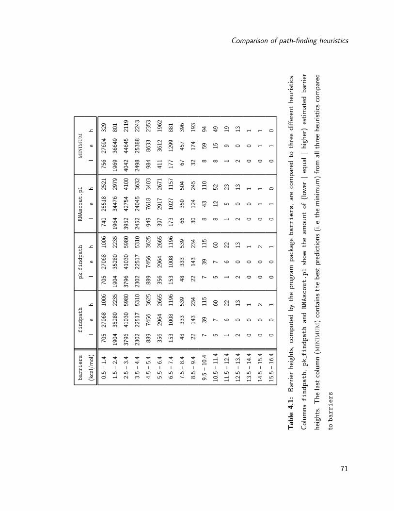
Comparison of path-finding heuristics
barriers
findpath
pkfindpath
RNAscout.pl
minimum
(kca
l/m
ol)
le
hl
eh
le
hl
eh
0.5
–1.
470
527
068
1006
705
2706
810
0674
025
518
2521
756
2769
432
9
1.5
–2.
419
0435
280
2235
1904
3528
022
3519
6434
476
2979
1969
3664
980
1
2.5
–3.
437
9641
030
5980
3796
4103
059
8039
5242
754
4100
4042
4464
521
19
3.5
–4.
423
0222
517
5310
2302
2251
753
1024
5224
045
3632
2498
2538
822
43
4.5
–5.
488
974
5636
2588
974
5636
2594
976
1834
0398
486
3323
53
5.5
–6.
435
629
6426
6535
629
6426
6539
729
1726
7141
136
1219
62
6.5
–7.
415
310
0811
9615
310
0811
9617
310
2711
5717
712
9988
1
7.5
–8.
448
333
539
4833
353
966
350
504
6745
739
6
8.5
–9.
422
143
234
2214
323
430
124
245
3217
419
3
9.5
–10
.47
3911
57
3911
58
4311
08
5994
10.5
–11
.45
760
57
608
1252
815
49
11.5
–12
.41
622
16
221
523
19
19
12.5
–13
.42
013
20
132
013
20
13
13.5
–14
.40
01
00
10
01
00
1
14.5
–15
.40
02
00
20
11
01
1
15.5
–16
.40
01
00
10
10
01
0
Table
4.1
:B
arrier
hei
ghts
,co
mpute
dby
the
prog
ram
pac
kage
barriers,
are
com
par
edto
thre
ediff
eren
theu
rist
ics.
Col
um
nsfindpath,pkfindpath
andRNAscout.pl
show
the
amou
nt
of(low
er|
equal
|hig
her
)es
tim
ated
bar
rier
hei
ghts
.T
he
last
colu
mn
(minimum
)co
nta
ins
the
bes
tpr
edic
tion
s(i.e
.the
min
imum
)from
allth
ree
heu
rist
ics
com
par
ed
tobarriers
71
4 Computational results
RNAscout.pl predicts more equal barrier heights and less higher barrier heights than the
direct path heuristics in general. The amount of lower estimated barrier heights is in-
creased to direct path heuristics, indicating that some of these estimations result from
indirect pseudoknotted intermediates that could not be found by direct path heuristics and
barriers.
The last column shows the minimum of all heuristic barrier height estimations. The differ-
ence to the best heuristic (RNAscout.pl) shows that there are barrier heights where the
direct path heuristics performed better than RNAscout.pl. These results are predominantly
caused by small local rearrangements. As an example, given a local minimum consisting of
a helix with the complementary strands A and B, and another minimum forms a slightly
shifted helix of same length A′ with B′, then the structures are neither neighbors within the
stacked helix move-set nor comprised in each other. RNAscout.pl will therefore not see
these conformations as neighbors; instead, it connects the structures with a transition state
that (in worst case) has no base-pair of both helices inserted. For such small rearrange-
ments, a direct path heuristic is usually sufficient. The set of pk findpath better/worse
predictions is therefore not completely included within the set of RNAscout.pl predictions.
The fact that there is no difference between the heuristics findpath and pk findpath,
might have two reasons: Firstly the interaction penalty for an initial pseudoknot base-pair
is 8.1 kcal/mol, which cannot be compensated by the insertion of small helix regions. Sec-
ondly, local rearrangements, such as the relocation of a bulge loop or the shift of a whole
helix region do not allow to form pseudoknot structures. Instead, pseudoknot transition
states occur predominantly between secondary structures that differ in whole helix regions,
such that pseudoknotted transition states allow the partial formation of both helices. Ap-
parently, within the RNAstrand data set, the amount of such distant rearrangements is
little or non-existent. However, differences between findpath and pk findpath can be
seen with lower pseudoknot penalties (data not shown). A pseudoknot penalty of 4.1
72
Comparison of path-finding heuristics
kcal/mol (i. e. the duplex initiation energy) shows a lot of lower barrier energies starting
when inspecting medium and high barriers from 6.4 to 16.4 kcal/mol.
The difference between barrier height predictions from the individual programs is shown in
figure 4.3. Figure 4.3a contains the same data as discussed in table 4.1, i. e. all attached
barriers computed by barriers (disregarding the barrier heights where recomputation
with RNAscout.pl failed). Figure 4.3b compares predictions for detached barrier heights,
i. e. heights that could not be determined by barriers, due to the limited amount of
suboptimal structures. For simplicity, we computed the minimum barrier height to the
MFE secondary structure for every detached barrier (again disregarding the barrier heights
where recomputation with RNAscout.pl failed).
Comparing the different programs in figure 4.3a, we see that the main variation between
barriers and all heuristics is concentrated to a small range. This range as a whole is shifted
to higher barrier estimations with increasing precomputed barrier heights. RNAscout.pl
results show that there are more outliers of very high estimated barrier heights. Interestingly,
we see differences when comparing the barrier heights computed by direct path heuristics, as
there are a few cases where indirect paths lower the barrier height. RNAscout.pl compared
to the direct path heuristics shows many better predictions.
Figure 4.3b also shows that pk findpath performs better at a small amount of refolding
paths. With increasing barrier heights, RNAscout.pl shows increasing deviations in both
lower and higher barrier predictions.
These observations underline that RNAscout.pl is susceptible to false barrier estimation
from local rearrangements that can be computed by findpath, but occasionally returns
very bad results with the automatically adjusted guiding stringency. Instead, direct path
heuristics show less bad estimations, but a higher amount of small differences. The mini-
mum of the heuristics should therefore give a good estimation of the real barrier heights.
73

4 Computational results
barriers
0 5 10 15 20 0 5 10 15 20
510
15
05
1015
20
findpath
pk_findpath
05
1015
20
5 10 15
05
1015
20
0 5 10 15 20
RNAscout.pl
(a) Correlation plot of barrier predictions
findpath
0 5 10 15 20
05
1015
20
05
1015
20
pk_findpath
0 5 10 15 20 0 5 10 15 20 25
05
1015
2025
RNAscout.pl
(b) Correlation plot of barrier predictions
Figure 4.3: Barrier heights computed by the different programs are compared to each
other. (a) compares all programs, (b) compares predictions for barrier heights that could
not be determined by barriers.
74

Comparison of kinetic simulations
The histograms in figure 4.4a depict the differences between barrier heights computed by
barriers and RNAscout.pl predictions. Apparently, the majority of predictions is equal.
The main differences between predicted barriers range from -2 to 2 kcal/mol, while the
amount of higher predicted barriers is greater than the amount of lower predicted barriers.
The histogram in figure 4.4b contains the difference between barriers and the minimum
over all heuristics. As expected, the amount of worse predicted barriers is smaller, the
amount of equal and better predicted structures is higher.
As a concluding remark of this section we see that RNAscout.pl does enhance the pre-
diction of barrier heights, but it is advisable to consider the pk findpath heuristic as an
upper bound for network generation. In contrast to the current approach, RNAscout.pl
would not stop network expansion if it has more than 500 RNA secondary structures, but
expand until at least the pk findpath barrier height is found. This, however, is too time
consuming for the evaluation of all barrier heights from the RNAstrand data set, as it would
require the variation of both network parameters γ and δ to keep the network size com-
putationally tractable. However, we will see in the following section that recomputation of
single barrier heights with variable parameters can strongly influence the performance of
RNAscout.pl.
4.3 Comparison of kinetic simulations
The following section compares the accuracy of heuristic RNAscout.pl networks with
coarse-grained barriers landscapes. Different coarse-grained landscapes from a manu-
ally selected sequence were generated with barriers and folding kinetics based on these
landscapes were calculated with treekin. The simulations have then been compared
to heuristic landscapes that consider solely the local minima obtained from barrier trees.
Saddle points are recomputed with all three heuristics, transition rates are calculated by
75

4 Computational results
−15 −10 −5 0 5 10 15
1e+
001e
+02
1e+
041e
+06
Difference of barrier heights
Cou
nt
(a) HRNAscout.pl − Hbarriers
−15 −10 −5 0 5 10 15
1e+
001e
+02
1e+
041e
+06
Difference of barrier heights
Cou
nt
(b) Hheuristics − Hbarriers
Figure 4.4: Difference of barrier height predictions. (a) RNAscout.pl against precom-
puted barriers from the barriers package. The majority of predictions is equal, main
differences range from -3.9 to 7.7 kcal/mol. (b) the minimum prediction of direct and
indirect path heuristics against the barriers package. The amount of equal predictions
increases significantly, while the amount of higher estimations is lower.
76

Comparison of kinetic simulations
Arrhenius kinetics as it is done in the RNAscout.pl algorithm (see section 3.2.3).
Subsequently, an RNAscout.pl network was generated from a manually selected starting
conformation and the MFE conformation. The network parameters δ and γ (see equa-
tion 3.15) were varied to measure their influence on the size of the generated network,
the minimum barrier height found and the refolding kinetics on subsequent treekin sim-
ulations. The results obtained from RNAscout.pl networks are then compared to an
exhaustively computed folding landscape from barriers.
Influence of the basins of attraction
To measure the accuracy of RNAscout.pl we searched the previously generated barrier
trees for small sequences with many energetically trapped local minima (i. e.minima with
high minimum barriers). To increase the complexity of the problem, the conformation we
start our simulations with should not be directly connected with the MFE conformation,
but should firstly lead to an energetically trapped intermediate structure and then refold
into the MFE secondary structure. The RNA folding landscape of the signal recognition
particle SRP 00209 [192] contains a path fulfilling this properties. Tables 4.2, 4.3a and 4.3b
represent three barrier trees with a minimum barrier height (HMIN) of 1, 3 and 5 kcal/mol,
respectively. The minimum free energy computed for SRP 00209 is -35.70 kcal/mol. The
energy range δ for RNAsubopt was set to 13.30 kcal/mol, which results in 5139059 struc-
tures up to a free energy of -22.40 kcal/mol. We decided to compute all barrier trees such
that they cover the local minimum structures up to a free energy of -31.80 kcal/mol, which
is the energy of the selected conformation we will start our simulations with.
As we have discussed in section 3.1.1, barriers returns a set of RNA secondary struc-
tures, where each conformation represents the minimum of a certain basin of attraction.
Rates between the local minima are calculated considering the internal equilibrium partition
77

4 Computational results
GGCCCCUACGUGGUGUCAUCUCGCUGAACUUCCCCCAGGACCGGAAGGUAGCAAGGGUAGGUGGGCUCUGGCAGGUGCGUGAGGGGUCUUCACGUUU
ID Structure (Ω) E(Ω) N H N H
1 ((((((((((((.(((((.((((((......(((.....(((....))).....)))..))))))...)))))..))))).)))))))......... -35.70 0 11.43 0 13.30
2 ((((((((((((.(((((.((((((......(((.....(((....))).....)))..))))))...)))))..)))))).))))))......... -35.40 1 2.30 1 2.30
3 ((((((((((((.(((((....(((..(((((((.....(((....))).....))).)))).)))..)))))..))))).)))))))......... -35.40 1 7.30 1 7.30
4 ((((((((((((.(((((....(((..(((((((.....(((....))).....))).)))).)))..)))))..)))))).))))))......... -35.10 3 2.30 3 2.30
5 ((((((((((((.(((((....(((..((((.(((....(((....))).....))).)))).)))..)))))..))))).)))))))......... -35.10 1 7.00 1 7.00
6 ((((((((((((.(((((....(((.(.((((((.....(((....))).....))).)))).)))..)))))..))))).)))))))......... -34.90 3 1.70 3 1.70
7 ((((((((((((.(((((....(((.(.((.(((.....(((....))).....))).)).).)))..)))))..))))).)))))))......... -34.90 3 3.60 3 3.60
8 ((((((((((((.(((((....(((..((((.(((....(((....))).....))).)))).)))..)))))..)))))).))))))......... -34.80 5 2.30 5 2.30
9 ((((((((((((.(((((.(((((....((.(((.....(((....))).....))).)))))))...)))))..))))).)))))))......... -34.70 1 1.60 1 1.60
10 ((((((((((((.(((((....(((.(.((((((.....(((....))).....))).)))).)))..)))))..)))))).))))))......... -34.60 4 1.70 4 1.70
11 ((((((((((((.(((((....(((.(.(((.(((....(((....))).....))).)))).)))..)))))..))))).)))))))......... -34.60 5 1.70 5 1.70
12 ((((((((((((.(((((....(((.(.((.(((.....(((....))).....))).)).).)))..)))))..)))))).))))))......... -34.60 7 2.30 7 2.30
13 ((((((((((((.(((((.(((((....((.(((.....(((....))).....))).)))))))...)))))..)))))).))))))......... -34.40 1 1.60 1 1.60
14 ((((((((((((.(((((....(((.(.(((.(((....(((....))).....))).)))).)))..)))))..)))))).))))))......... -34.30 8 1.70 8 1.70
15 ((((((((((((.(((((.((((((.......(((....(((....))).....)))..))))))...)))))..))))).)))))))......... -33.90 1 5.70 1 6.00
16 ((((((((((((.(((((.((((((.......(((....(((....))).....)))..))))))...)))))..)))))).))))))......... -33.60 15 2.30 15 2.30
...
47 ((((((((((((.(((((.((((((...(((((.........)))))............))))))...)))))..))))).)))))))......... -31.90 1 7.60 1 7.60
48 ((((((((((((.(((((.(((((....((...(((...(((....))).....))).)))))))...)))))..))))).)))))))......... -31.90 19 2.30 19 2.30
49 ((((((((((((.(((((.(((.....((((.(((....(((....))).....))).)))))))...)))))..)))))).))))))......... -31.90 36 2.30 36 2.30
50 ((((((((((((.(((((...(.(...(((((((.....(((....))).....))).))))).)...)))))..)))))).))))))......... -31.90 3 2.10 3 2.10
51 ((((((((((((.(((((...(.(...((((.(((....(((....))).....))).))))).)...)))))..))))).)))))))......... -31.90 5 2.10 5 2.10
52 ((((((((((((.(((((.(((((.....(((((.....(((....))).....))).)))))))...)))))..)))))).))))))......... -31.80 1 1.40 1 1.40
53 ((((((((((((.(((((.(((((.....((.(((....(((....))).....))).)))))))...)))))..))))).)))))))......... -31.80 15 1.30 15 1.30
54 ((((((((((((.(((((....((((..(((((.........))))).))))..((((......)))))))))..))))).)))))))......... -31.80 47 7.00 47 7.00
Table 4.2: An energetically sorted set of local minima from the signal recognition particle
SRP 00209. The RNA sequence is shown above the table. The first five columns show
standard output of the program package barriers with a minimum barrier height HMIN
of 1 kcal/mol. For each Structure(Ω), the free energy (E(Ω)) and the minimum barrier
height (H) to the next neighboring structure (N) is shown. N refers to the ID of the
(neighboring) structure. The last two columns, the second (N,H) pair, is recomputed with
the heuristics discussed in section 3.2 and represents the minimum of their predictions. Bold
values underline inaccuracy of the heuristics.
78

Comparison of kinetic simulations
GGCCCCUACGUGGUGUCAUCUCGCUGAACUUCCCCCAGGACCGGAAGGUAGCAAGGGUAGGUGGGCUCUGGCAGGUGCGUGAGGGGUCUUCACGUUU
ID Structure (Ω) E(Ω) N H N H
1 ((((((((((((.(((((.((((((......(((.....(((....))).....)))..))))))...)))))..))))).)))))))......... -35.70 0 13.30 0 13.30
2 ((((((((((((.(((((....(((..(((((((.....(((....))).....))).)))).)))..)))))..))))).)))))))......... -35.40 1 7.30 1 7.30
3 ((((((((((((.(((((....(((..((((.(((....(((....))).....))).)))).)))..)))))..))))).)))))))......... -35.10 1 7.00 1 7.00
4 ((((((((((((.(((((....(((.(.((.(((.....(((....))).....))).)).).)))..)))))..))))).)))))))......... -34.90 2 3.60 2 3.60
5 ((((((((((((.(((((.((((((.......(((....(((....))).....)))..))))))...)))))..))))).)))))))......... -33.90 1 5.70 1 6.00
6 ((((((((((((.(((((.((((((.....(((......(((....))).....)))..))))))...)))))..))))).)))))))......... -33.30 1 4.20 1 5.20
7 ((((((((((((.(((((.((((((........(((...(((....))).....)))..))))))...)))))..))))).)))))))......... -33.30 1 6.00 1 7.00
8 ((((((((((((.(((((....(((..((((..(((...(((....))).....))).)))).)))..)))))..))))).)))))))......... -32.80 1 5.50 3 5.50
9 ((((((((((((.(((((.(((.....(((((((.....(((....))).....))).)))))))...)))))..))))).)))))))......... -32.50 2 4.20 2 4.20
10 ((((((((((((.(((((.(((((((.....(((.....(((....))).....)))))).))))...)))))..))))).)))))))......... -32.20 1 3.40 1 3.40
11 ((((((((((((.(((((.(((.....((((.(((....(((....))).....))).)))))))...)))))..))))).)))))))......... -32.20 1 4.20 2 4.20
12 ((((((((((((.(((((.((((((...(((((.........)))))............))))))...)))))..))))).)))))))......... -31.90 1 7.60 1 7.60
13 ((((((((((((.(((((....((((..(((((.........))))).))))..((((......)))))))))..))))).)))))))......... -31.80 12 7.00 12 7.00
(a) HMIN = 3
GGCCCCUACGUGGUGUCAUCUCGCUGAACUUCCCCCAGGACCGGAAGGUAGCAAGGGUAGGUGGGCUCUGGCAGGUGCGUGAGGGGUCUUCACGUUU
ID Structure (Ω) E(Ω) N H N H
1 ((((((((((((.(((((.((((((......(((.....(((....))).....)))..))))))...)))))..))))).)))))))......... -35.70 0 13.30 0 13.30
2 ((((((((((((.(((((....(((..(((((((.....(((....))).....))).)))).)))..)))))..))))).)))))))......... -35.40 1 7.30 1 7.30
3 ((((((((((((.(((((....(((..((((.(((....(((....))).....))).)))).)))..)))))..))))).)))))))......... -35.10 1 7.00 1 7.00
4 ((((((((((((.(((((.((((((.......(((....(((....))).....)))..))))))...)))))..))))).)))))))......... -33.90 1 5.70 1 6.00
5 ((((((((((((.(((((.((((((........(((...(((....))).....)))..))))))...)))))..))))).)))))))......... -33.30 1 6.00 1 7.00
6 ((((((((((((.(((((....(((..((((..(((...(((....))).....))).)))).)))..)))))..))))).)))))))......... -32.80 1 5.50 3 5.50
7 ((((((((((((.(((((.((((((...(((((.........)))))............))))))...)))))..))))).)))))))......... -31.90 1 7.60 1 7.60
8 ((((((((((((.(((((....((((..(((((.........))))).))))..((((......)))))))))..))))).)))))))......... -31.80 7 7.00 7 7.00
(b) HMIN = 5
Table 4.3: An energetically sorted set of local minima from the signal recognition particle
SRP 00209. The RNA sequence is shown above both tables. The first five columns show
standard output of the program package barriers with a minimum barrier height HMIN
of 3 kcal/mol (a) and 5 kcal/mol (b). For each Structure(Ω), the free energy (E(Ω)) and
the minimum barrier height (H) to the next neighboring structure (N) is shown. N refers
to the ID of the neighboring structure. The last two columns, the second (N,H) pair, is
recomputed with the heuristics discussed in section 3.2 and represents the minimum of their
predictions. Bold values underline inaccuracy of the heuristics.
79

4 Computational results
functions of the corresponding basins. treekin simulations based on the three different
coarse-grained landscapes can be seen in the first column of figure 4.5. The ID of the
trajectory corresponds to the ID of the structure in tables 4.2 4.3a and 4.3b.
Generally the results can be split into three parts. The first addresses the starting confor-
mation, which has ID 54, 13 and 8 in the three different barrier trees. Independently of
the coarse-graining, the population of this structure behaves similarly, but decreases faster
when increasing the minimum barrier height. Supposedly, aggregation of small basins to one
big gradient basin alters the influence of small rates (high barriers) to neighboring basins
relative to high rates (small barriers) within the equilibrium distribution of the merged
basins.
The second part of the simulation regards the population of intermediate states. The
simulation on the most detailed landscape (HMIN = 1) behaves as expected. While the
population of the starting basin decreases, the transition basin (table 4.2: 47) increases.
In contrast, HMIN = 3 and HMIN = 5 simulations compute the MFE secondary structure
basin as highest populated intermediate. The population of the transition basin (table 4.3a:
12 and table 4.3b: 7) is comparatively low.
The last difference can be seen in the equilibrium distribution of the gradient basins. The
MFE conformation basin is highest populated in every simulation, the rest of the basins
are not sorted according to their best local energy, as the amount of structures within the
basins plays a crucial role. Because small basins are merged into one basin when raising the
minimum barrier height, the remaining representing structures are distributed differently.
For this reason, the equilibrium distribution is strongly dependent on the minimum barrier
height.
The simulations considering gradient-basins are now compared to simulations of a heuristic
image of the folding landscape. The gradient basins were sacrificed and the local minima
80
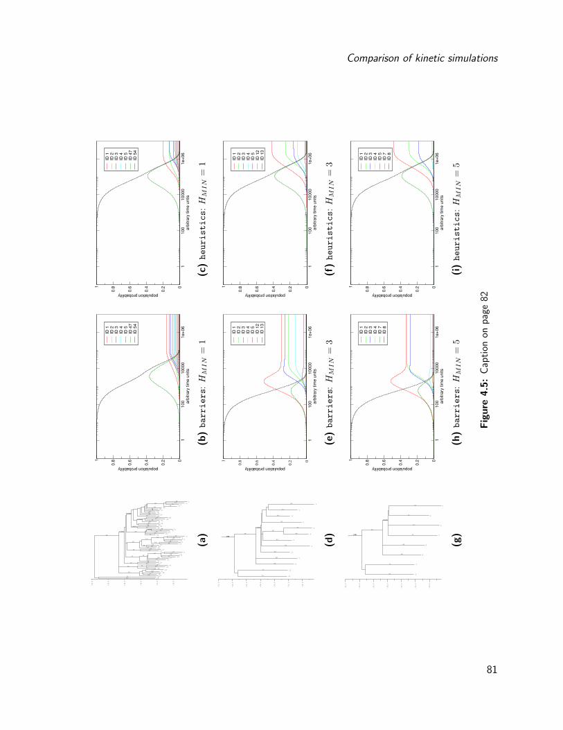
Comparison of kinetic simulations
12
3
4
5
6
7
8
9
10
11
12
13
14
1516
17
18
19
20
21
22
23
24
25
26
27
28
29
30
31
32
33
34
35
36
37
38
39
40
41
42
43
44
45
46
47
48
49
50
51
52
53
54
-34.0
-32.0
-30.0
-28.0
-26.0
-24.0
1.72.2
2.32.6
1.6
1.72.2
1.72.2
1.6
1.72.2
2.32.6
1.0
1.5
2.32.6
2.5
1.6
2.3
1.8
2.0
2.5
0.599998
2.32.6
2.32.6
1.4
1.31.5
2.3
1.72.2
1.8
1.8
1.3
1.4
1.72.2
1.8
0.6
1.2
1.8
2.32.6
2.3
2.3
2.1
1.0
2.1
2.32.6
2.32.6
2.3
1.1
2.3
2.32.6
0.700001
0.800001
1.6
1.5
2.3
0.599998
1.7
1.6
2.3
0.700001
2.5
7.07.1
3.0
(a)
1100
10000
1e+
06
arb
itra
ry tim
e u
nits
0
0.2
0.4
0.6
0.81
population probability
ID 1
ID 2
ID 3
ID 4
ID 5
ID 4
7ID
54
(b)barriers:
HM
IN
=1
1100
10000
1e+
06
arb
itra
ry tim
e u
ntis
0
0.2
0.4
0.6
0.81
population probability
ID 1
ID 2
ID 3
ID 4
ID 5
ID 4
7ID
54
(c)heuristics:
HM
IN
=1
1
2
3
4
5
6
7
8
9
10
11
12
13
-34.0
-32.0
-30.0
-28.0
-26.0
-24.0
-22.0
3.6
4.1
4.2
6.6
3.4
4.2
3.0
5.7
7.0
4.2
6.0
0.700001
5.5
7.0
7.1
3.0
1.9011.901
(d)
1100
10000
1e+
06
arb
itra
ry tim
e u
nits
0
0.2
0.4
0.6
0.81
population probability
ID 1
ID 2
ID 3
ID 4
ID 5
ID 1
2ID
13
(e)barriers:
HM
IN
=3
1100
10000
1e+
06
arb
itra
ry tim
e u
nits
0
0.2
0.4
0.6
0.81
population probability
ID 1
ID 2
ID 3
ID 4
ID 5
ID 1
2ID
13
(f)heuristics:
HM
IN
=3
1
2
3
4
5
6
7
8
-34.0
-32.0
-30.0
-28.0
-26.0
-24.0
-22.0
5.7
7.5
7.3
7.0
6.0
0.800001
5.5
7.0
7.1
3.0
1.9011.901
(g)
1100
10000
1e+
06
arb
itra
ry tim
e u
nits
0
0.2
0.4
0.6
0.81
population probability
ID 1
ID 2
ID 3
ID 4
ID 7
ID 8
(h)barriers:
HM
IN
=5
1100
10000
1e+
06
arb
itra
ry tim
e u
nits
0
0.2
0.4
0.6
0.81
population probability
ID 1
ID 2
ID 3
ID 4
ID 5
ID 7
ID 8
(i)heuristics:
HM
IN
=5
Fig
ure
4.5
:Cap
tion
onpag
e82
81
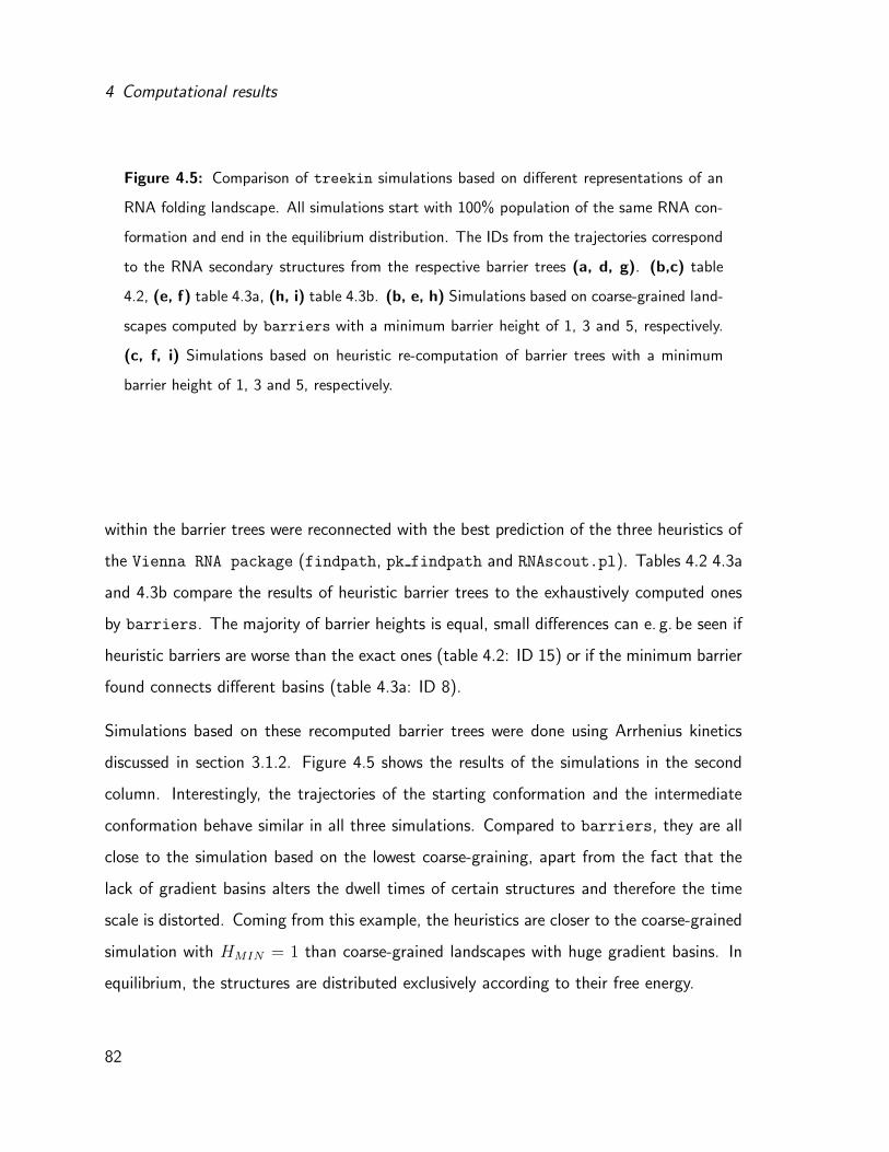
4 Computational results
Figure 4.5: Comparison of treekin simulations based on different representations of an
RNA folding landscape. All simulations start with 100% population of the same RNA con-
formation and end in the equilibrium distribution. The IDs from the trajectories correspond
to the RNA secondary structures from the respective barrier trees (a, d, g). (b,c) table
4.2, (e, f) table 4.3a, (h, i) table 4.3b. (b, e, h) Simulations based on coarse-grained land-
scapes computed by barriers with a minimum barrier height of 1, 3 and 5, respectively.
(c, f, i) Simulations based on heuristic re-computation of barrier trees with a minimum
barrier height of 1, 3 and 5, respectively.
within the barrier trees were reconnected with the best prediction of the three heuristics of
the Vienna RNA package (findpath, pk findpath and RNAscout.pl). Tables 4.2 4.3a
and 4.3b compare the results of heuristic barrier trees to the exhaustively computed ones
by barriers. The majority of barrier heights is equal, small differences can e. g. be seen if
heuristic barriers are worse than the exact ones (table 4.2: ID 15) or if the minimum barrier
found connects different basins (table 4.3a: ID 8).
Simulations based on these recomputed barrier trees were done using Arrhenius kinetics
discussed in section 3.1.2. Figure 4.5 shows the results of the simulations in the second
column. Interestingly, the trajectories of the starting conformation and the intermediate
conformation behave similar in all three simulations. Compared to barriers, they are all
close to the simulation based on the lowest coarse-graining, apart from the fact that the
lack of gradient basins alters the dwell times of certain structures and therefore the time
scale is distorted. Coming from this example, the heuristics are closer to the coarse-grained
simulation with HMIN = 1 than coarse-grained landscapes with huge gradient basins. In
equilibrium, the structures are distributed exclusively according to their free energy.
82

Comparison of kinetic simulations
Network size
δ
γ2.0 1.0 0.9 0.8 0.7 0.6 0.5 0.4 0.3 0.2 0.1 0.0
0.1 18 37 38 39 42 54 75 78 91 136 264 479
0.5 21 40 41 41 54 74 81 113 125 171 347 592
1.0 27 46 51 59 75 85 111 126 157 272 479 1021
1.5 28 52 69 81 103 109 133 171 226 362 633 1466
2.0 31 79 90 108 126 138 168 218 372 519 847
2.5 38 110 117 130 149 195 252 338 495 627 1140
3.0 54 131 143 167 196 246 319 443 583 891 1615
3.5 69 156 172 191 256 315 431 584 789 1129
4.0 80 176 203 259 297 436 561 751 984 1731
4.5 91 221 242 310 428 560 738 927 1451
5.0 104 256 328 472 548 727 951 1297
Table 4.4: Amount of structures within the RNAscout.pl network dependent on the user
defined parameters δ and γ. Background colors indicate the predicted barrier height. Dark
gray: H = 9.40 kcal/mol; white: H = 7.50 kcal/mol.
RNAscout.pl compared to an exhaustive computed folding landscape
We will now evaluate the RNAscout.pl output if only the starting structure Ωi and the
MFE structure Ωj from figure 4.5 are given. First of all, table 4.4 shows the influence of
γ and δ for this specific network. In this case, the graph is already connected (i.e. there
is a path Πj⇐i) with δ = 0.1 kcal/mol and γ = 2.0, which are very restrictive parameters.
The estimated minimum barrier height, however, is 9.40 kcal/mol with these parameters.
Expanding the network (e. g. with the parameters δ = 2.5 kcal/mol and γ = 0.4) lowers
the estimated barrier height to 7.50 kcal/mol.
83

4 Computational results
We can expect that the simulations based on networks with estimated barrier heights of
9.40 kcal/mol will compute a longer refolding time, than those with a minimum barrier
height of 7.50 kcal/mol. We will refer to changes in the refolding time as qualitative
changes, that are very important to measure the efficiency of a refolding path.
On the other hand, the higher the amount of vertices, the more we converge to the results
of a simulation in the full conformation space. This convergence should predominantly
influence the population size of individual structures in respect to similar suboptimal struc-
tures, but should not influence the refolding time between different local minima. These
changes will be seen as quantitative changes that are of little importance to measure the
efficiency of a refolding path, as the refolding time is not affected. A quantitative de-
scription of population density in a heuristically estimated conformation space is risky, as
energetically good but structurally distant conformations might not be found and the basins
of attraction are not included for the individual local minima. We will therefore focus on a
good qualitative description with respect to the time scale.
Figure 4.6a shows changes in the population of starting and MFE trajectory for a constant
guiding stringency γ = 0.4 and the variation of the energy range δ from 0.1 kcal/mol to
5.0 kcal/mol. The simulation based on the smallest network (δ = 0.1 kcal/mol), shows
both starting and MFE trajectories mainly between 90% and 100%, due to the low amount
of competitive structures. Small expansions of the network (up to δ = 2.0 kcal/mol) do
not influence the barrier height and thus, weakly influence the trajectories. We can see
quantitative changes in the population density and small qualitative changes in the refolding
time.
Further network expansion to δ = 2.5 kcal/mol lowers the minimum barrier height and
heavily influences the refolding time. The quantitative changes, in contrast, do only in-
fluence the time period when the new transition state is detected. In equilibrium, the
84

Comparison of kinetic simulations
population of the MFE secondary structure remains constant. Even higher values of δ,
up to the biggest network generated with γ = 0.4 and δ = 5.0 kcal/mol solely result in
quantitative changes. At δ = 3.5 kcal/mol, the population of the MFE secondary structure
in the equilibrium decreases and finally with δ = 5.0 a new structure is included that differs
from the starting structure in solely two base-pairs. This energetically worse, but nearly
equal structure populates immediately, but does not influence the refolding time.
Figure 4.6b shows a treekin simulation based on the most detailed rate matrix we can
compute with barriers. The rates within the matrix are not rates connecting macro-
states (basins of attraction) but micro-states (single structures). Usually a sequence of
97 nucleotides length is too long to calculate full dynamics. However, in this case, the
structures within our energy range do all have a constant part of 50 nucleotides. The
remaining dynamic part of 47 nucleotides is small enough to compute micro-rates. We find
that this full simulation predicts a similar behavior of the starting trajectory compared to the
RNAscout.pl network with δ = 5.0. The first upcoming sequence was previously merged
into the gradient basin of the starting sequence (see figure 4.5). The population of the
MFE secondary structure seems very small, which is expected if all suboptimal structures
are considered without being merged into gradient basins. Note that the timescale in
figure 4.6a and 4.6b is slightly different, but the behavior of the trajectories is comparable.
While figure 4.6a shows the changes with increasing energy range and a guiding potential
of γ = 0.4, table 4.5 shows the computed distances of the trajectories (see equation 3.17)
for γ ranging from 2.0 to 0.4. Similarly to γ = 0.4, the main changes in the positions of
the trajectories are found when a lower barrier is obtained. If the barrier height remains
constant, there are only small qualitative changes in the population density. The last change
including the slightly modified, energetically worse starting sequence is only found with the
smallest guiding stringency. We therefore conclude that simulations based on networks that
found the lowest barrier heights are sufficient for a qualitative description of the refolding
85

4 Computational results
0.1 10 1000 1e+05 1e+07arbitrary time scale
0
0.2
0.4
0.6
0.8
1popula
tion p
robabili
ty
E: 0.1E: 0.5E: 1.0E: 1.5E: 2.0E: 2.5E: 3.0E: 3.5E: 4.0E: 4.5E: 5.0
δδδδδδδδδδδ
(a) RNAscout.pl – γ = 0.4
0.1 10 1000 1e+05 1e+07arbitrary time scale
0
0.2
0.4
0.6
0.8
1
popula
tion p
robabili
ty
(b) barriers
Figure 4.6: Caption on page 87
86

Evaluation of a synthetic riboswitch
Figure 4.6: treekin simulations of the SRP 00209 RNA. (a) Comparison of eleven simu-
lations based on different RNAscout.pl networks. While the guiding potential is constant
with γ = 0.4, the energy range δ varies from 0.1 kcal/mol up to 5.0 kcal/mol. For each
simulation, the starting and MFE trajectories are shown (in the same color). The two struc-
ture comics are the starting and MFE structure, respectively. Blue base-pairs in the MFE
structure remain constant during the simulation, red base-pairs are different from the start-
ing conformation. (b) A treekin simulation based on a folding landscape that considers
micro-rates (between single structures) instead of macro-rates (between gradient basins).
Structures correspond to the closest trajectories. Blue base-pairs are those initially formed
by the starting structure. The first upcoming sequence has one different base-pair (marked
in green), new base-pairs formed by the MFE secondary structure are shown in red..
time. In case of guiding stringency γ = 0.4 we need an energy range δ of at least 2.5
kcal/mol.
Interestingly, this section showed that the coarse-graining level of barriers, even though
it just merges gradient basins, has a high impact on subsequent simulations. In contrast,
heuristic landscapes that consider solely the local minima obtained from barrier trees show
a smaller impact on subsequent simulations.
4.4 Evaluation of a synthetic riboswitch
As discussed in section 1.4, the primary incitement to implement the RNAscout.pl algo-
rithm was to provide a basis for the in silico evaluation of synthetic riboswitches.
The basic concept of the riboswitch published by Isaacs et al. [1] is to use two sequences
that fold into certain stable structures as soon as they are transcribed. The cis-repressed
87
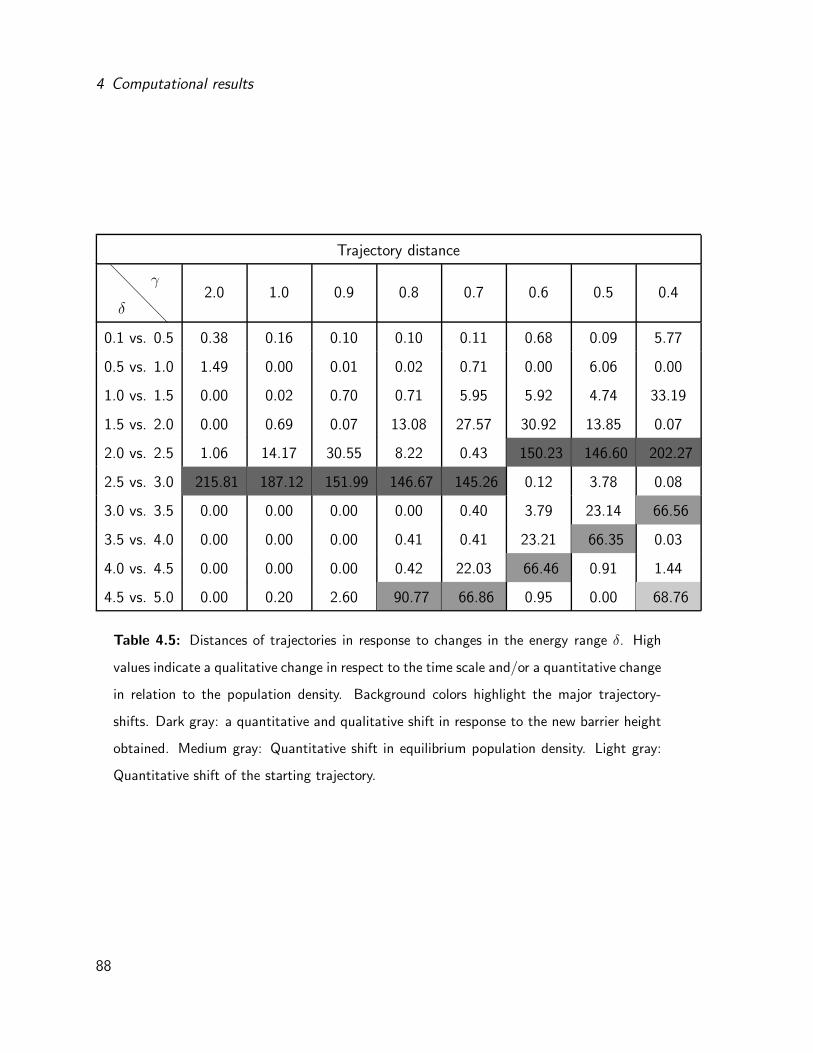
4 Computational results
Trajectory distance
δ
γ2.0 1.0 0.9 0.8 0.7 0.6 0.5 0.4
0.1 vs. 0.5 0.38 0.16 0.10 0.10 0.11 0.68 0.09 5.77
0.5 vs. 1.0 1.49 0.00 0.01 0.02 0.71 0.00 6.06 0.00
1.0 vs. 1.5 0.00 0.02 0.70 0.71 5.95 5.92 4.74 33.19
1.5 vs. 2.0 0.00 0.69 0.07 13.08 27.57 30.92 13.85 0.07
2.0 vs. 2.5 1.06 14.17 30.55 8.22 0.43 150.23 146.60 202.27
2.5 vs. 3.0 215.81 187.12 151.99 146.67 145.26 0.12 3.78 0.08
3.0 vs. 3.5 0.00 0.00 0.00 0.00 0.40 3.79 23.14 66.56
3.5 vs. 4.0 0.00 0.00 0.00 0.41 0.41 23.21 66.35 0.03
4.0 vs. 4.5 0.00 0.00 0.00 0.42 22.03 66.46 0.91 1.44
4.5 vs. 5.0 0.00 0.20 2.60 90.77 66.86 0.95 0.00 68.76
Table 4.5: Distances of trajectories in response to changes in the energy range δ. High
values indicate a qualitative change in respect to the time scale and/or a quantitative change
in relation to the population density. Background colors highlight the major trajectory-
shifts. Dark gray: a quantitative and qualitative shift in response to the new barrier height
obtained. Medium gray: Quantitative shift in equilibrium population density. Light gray:
Quantitative shift of the starting trajectory.
88

Evaluation of a synthetic riboswitch
RNA (crRNA) needs to have a conformation with a blocked ribosome binding site (RBS)
and a loop interaction motive. The structure of the trans activation RNA (taRNA) must
expose an interaction motive complementary to the crRNA (see figure 1.2). Both structures
should be energetically stable if transcribed independently, but rearrange fast if they are
transcribed together. Isaacs et al. have shown that their two synthetic RNA sequences are
functional in Escherichia coli. Here we will kinetically evaluate the RNA molecules with
RNAscout.pl.
For two reasons, the refolding time cannot be estimated by barriers. Firstly, the maximum
of structures that barriers can handle is around 107. For our sequence this means that we
are allowed to increase the energy range to about 12 kcal/mol. However, within this energy
range there is no energetic barrier. Instead, the findpath heuristic estimates a barrier
height of 17.10 kcal/mol. The second problem is shown in figure 3.5. As the best refolding
path has a pseudoknotted intermediate, it is not predictable by conventional structure
prediction. The pk findpath barrier for our example is at 9.20 kcal/mol.
Table 4.6 shows the influence of γ and δ on the size of the generated network and the
changes in the starting and MFE trajectories during different treekin simulations. Both
RNA molecules together are 126 nucleotides long and they can fold into very distant
conformations. The set of energetically good structures within Qpk is therefore very high,
such that a guiding stringency γ = 1.8 in combination with an energy range δ = 0.1
kcal/mol already results in a heuristic Qpk network of 745 vertices. The minimum barrier
height found is always 9.20 kcal/mol, which is exactly the barrier height predicted by
pk findpath. The trajectory distances are computed using equation 3.17. All starting and
MFE trajectories are very similar, independently of the size of the generated network. Higher
distances between trajectories (such as γ: 3.5 and δ: 2.5 vs. 3.0) are small qualitative
changes concerning the population density (data not shown).
89
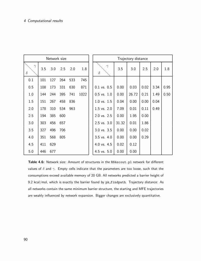
4 Computational results
Network size Trajectory distance
δ
γ3.5 3.0 2.5 2.0 1.8
δ
γ3.5 3.0 2.5 2.0 1.8
0.1 101 127 264 533 745
0.5 108 173 331 630 871 0.1 vs. 0.5 0.00 0.03 0.02 3.34 0.95
1.0 144 244 395 741 1022 0.5 vs. 1.0 0.00 26.72 0.21 1.49 0.50
1.5 151 267 458 836 1.0 vs. 1.5 0.04 0.00 0.00 0.04
2.0 178 310 534 963 1.5 vs. 2.0 7.09 0.01 0.11 0.49
2.5 194 385 600 2.0 vs. 2.5 0.00 1.95 0.00
3.0 303 456 657 2.5 vs. 3.0 31.32 0.01 1.86
3.5 327 496 706 3.0 vs. 3.5 0.00 0.00 0.02
4.0 351 568 805 3.5 vs. 4.0 0.00 0.00 0.29
4.5 411 629 4.0 vs. 4.5 0.02 0.12
5.0 446 677 4.5 vs. 5.0 0.00 0.00
Table 4.6: Network size: Amount of structures in the RNAscout.pl network for different
values of δ and γ. Empty cells indicate that the parameters are too loose, such that the
consumptions exceed available memory of 20 GB. All networks predicted a barrier height of
9.2 kcal/mol, which is exactly the barrier found by pk findpath. Trajectory distance: As
all networks contain the same minimum barrier structure, the starting and MFE trajectories
are weakly influenced by network expansion. Bigger changes are exclusively quantitative.
90
Evaluation of a synthetic riboswitch
Figure 4.7a shows a summary of trajectories computed from a network with γ = 2.5 and
and δ ranging from 0.1 up to 4.0. As discussed above, there are no significant changes
within the different simulations. We can therefore assume that the heuristic Qpk networks
are a sufficient approximation of the full Qpk. Figure 4.7b shows the full output for γ = 2.5
and δ = 4.0. We find that the intermediate state predicted by RNAscout.pl is indeed
similar to the transition state published by Isaacs et al.
91
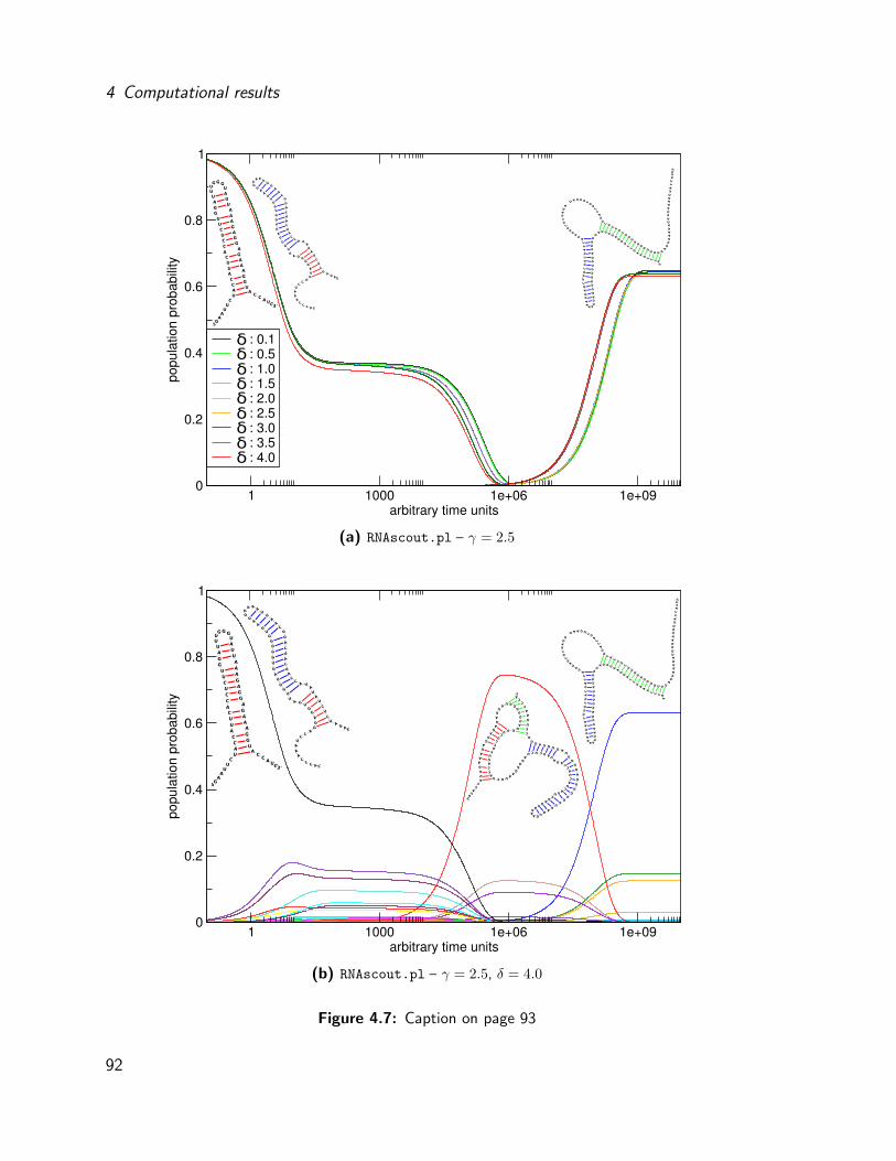
4 Computational results
0
0.2
0.4
0.6
0.8
1
popula
tion p
robabili
ty
E: 0.1E: 0.5E: 1.0E: 1.5E: 2.0E: 2.5E: 3.0E: 3.5E: 4.0
1 1000 1e+06 1e+09arbitrary time units
δδδδδδδδδ
(a) RNAscout.pl – γ = 2.5
0
0.2
0.4
0.6
0.8
1
popula
tion p
robabili
ty
1 1000 1e+06 1e+09arbitrary time units
(b) RNAscout.pl – γ = 2.5, δ = 4.0
Figure 4.7: Caption on page 93
92
Evaluation of a synthetic riboswitch
Figure 4.7: treekin simulations of heuristically estimated riboswitch folding landscapes.
(a): Comparison of nine simulations from RNAscout.pl networks in respect to a change
of the energy range δ. For each simulation, starting and MFE trajectories are shown (same
color). The simulation starts with two independently folded RNA conformations (see squig-
gle plots). The MFE secondary structure is an RNA duplex. Blue base-pairs remain constant
during the simulation, red base-pairs are opened an green base-pairs are closed. (b): Full
output of the treekin simulation with parameters γ = 2.5 and δ = 4.0 kcal/mol. Ad-
ditionally to starting and MFE structures, we see the squiggle plot of the most populated
intermediate structure. The green base-pairs form a pseudoknot interaction with a hairpin
loop. When refolding into the MFE secondary structure, red base-pairs open and green
base-pairs close consecutively.
93
5 Conclusion & Perspective
We have discussed that the amount of suboptimal RNA secondary structures (i. e. the con-
formation space) for a given molecule increases exponentially with sequence length. The
exhaustive computation of an RNA conformation space is therefore impossible for long
RNA molecules. Current algorithms restrict the conformation space to a subset of com-
putationally tractable, biologically reliable RNA secondary structures. These algorithms,
however, neglect certain natural RNA secondary structure motives (e. g. pseudoknots), that
have comparatively low impact on the MFE secondary structure prediction, but may have
a significant impact on folding kinetics.
The RNAscout.pl heuristic has been implemented to compute folding kinetics between
two RNA secondary structures including a wider set of RNA conformations, so called bi-
secondary structures. Our approach generates a heuristic image of the underlying confor-
mation space, bounded by two parameters. The energy range defines the set of energetically
relevant conformations, the guiding stringency excludes conformations that are structurally
distant from the input structures. Based on this heuristic image, we can estimate refolding
kinetics of both large RNA molecules and RNA molecules that are able to form pseudoknot
conformations.
94

Discussion of Results
5.1 Discussion of Results
Inspection of a well established data set of RNA sequences (from the RNAstrand database)
has shown that the majority of RNA molecules have lower barrier heights than shuffled
sequences with the same dinucleotide content. This leads to the assumption that RNA
molecules are optimized, such that they are able to fold into their MFE secondary struc-
ture quickly. However, we have also seen that it is not possible to compute the maximum
barrier height of RNA folding landscapes from long RNA sequences exhaustively. Further-
more, estimation of barriers with direct path heuristics is only reliable for small structural
arrangements up to a barrier height of 6.4 kcal/mol.
The predictions from pk findpath are predominantly equal to those from findpath, sug-
gesting that the inspected RNA molecules do not tend to form pseudoknotted intermediates
on direct paths. However, lowering the pseudoknot penalty shows different results. A better
energy model for pseudoknot interactions would therefore be highly appreciated.
The parameters of RNAscout.pl need to be adjusted carefully dependent on the type of
refolding path. Stringent parameters might exclude important structures and therefore
result in bad estimations of folding kinetics, loose parameters result in a computationally
intractable set of RNA conformations. Recomputation of precomputed barrier heights has
shown that automatic adjustment of the guiding stringency is often not sufficient, but
RNAscout.pl performs better than direct path heuristics in general.
When inspecting single refolding pathways, the variation of both parameters usually allows
to compute heuristic estimations of a conformation space that are sufficient to compute
folding kinetics. We have seen this in the case of a manually selected sequence from
the RNAstrand database. The quantitative description of population probabilities is not
possible, as we cannot estimate basins of attraction based on single local minimum con-
95

5 Conclusion & Perspective
formations. The qualitative description of the refolding time does also vary compared to
full simulations, but allows to quantify the influence of certain intermediate states. The
simulation of a synthetic riboswitch in response to its activating RNA molecule has un-
derlined the importance of the assumed intermediate state. This supports the ability of
RNAscout.pl to generate reliable heuristic images of the conformation space.
5.2 Perspective – Synthetic riboswitches
Due to the cellular function of RNA as a regulatory molecule, utilization of artificial RNA
is of great importance in a (synthetic) cell. The small section of optimized RNA-triggered
RNA switches allows a fast and versatile regulation of gene expression. In the simple case,
given by Isaacs et al. [1], one taRNA refolds one crRNA. This model can easily be expanded
such that various taRNAs are able to induce expression of different crRNAs.
Another interesting aspect concerning the utilization of RNA triggered switches is shown
by Friedland et al. [101]. They presented a method to initiate translation of crRNA in
response to different amounts of Arabinose pulses. Such models are very interesting in
respect to time management within a synthetic cell.
Based on the ability of RNAscout.pl to quantify the refolding time of riboswitches, it should
be possible to optimize refolding paths of certain RNA molecules by selective mutations.
However, the first step towards new synthetic riboswitches is the in silico design. A potent
approach to this has been shown by Flamm et al. in 2001 [189]. The algorithm of
switch.pl1 designs RNA sequences that are compatible with two different input structures.
In a nutshell, an initially random RNA sequence is iteratively optimized to enhance the
stability of both structures. In combination with RNAscout.pl one might establish a
1part of the Vienna RNA package
96

Perspective – Synthetic riboswitches
computational setup that suggests selected mutations, improving the refolding potential
between the generated RNA secondary structures. The combination of switch.pl and
RNAscout.pl could therefore lead to a efficient tool for both the design and evaluation of
synthetic RNA molecules that may form complex networks in synthetic biology.
97

A Appendix
98

ACCCAAAUCCAGGAGGUGAUUGGUAGUGGUGGUUAAUGAAAAUUAACUUACUACUACCAUAUAUCUCUAGA&GAAUUCUACCAUUCACCUCUUGGAUUUGGGUAUUAAAGAGGAGAAAGGUACCAUG
...........(((((((..(((((((((((((((((....)))))).)))))))))))..)))))))...&......((((.(((.((((((.(((......))).)))))).))).))))..... -42.40
...........(((((((..(((((((((((((((((....)))))).)))))))))))..)))))))...&.......(((.(((.((((((.(((......))).)))))).))).)))...... -41.10
...........(((((((..(((((((((((((((((....)))))).)))))))))))..)))))))...&........((.(((.((((((.(((......))).)))))).))).))....... -40.30
...........(((((((..(((((((((((((((((....)))))).)))))))))))..)))))))...&.........(.(((.((((((.(((......))).)))))).))).)........ -36.50
...........(((((((..(((((((((((((((((....)))))).)))))))))))..)))))))...&...........(((.((((((.(((......))).)))))).))).......... -37.20
............((((((..(((((((((((((((((....)))))).)))))))))))..))))))....&...........(((.((((((.(((......))).)))))).))).......... -36.80
............((((((..(((((((((((((((((....)))))).)))))))))))..))))))....&............((.((((((.(((......))).)))))).))........... -35.60
............((((((..(((((((((((((((((....)))))).)))))))))))..))))))....&.............(.((((((.(((......))).)))))).)............ -34.00
............((((((..(((((((((((((((((....)))))).)))))))))))..))))))....&...............((((((.(((......))).)))))).............. -35.40
............(((((...(((((((((((((((((....)))))).)))))))))))...)))))....&...............((((((.(((......))).)))))).............. -34.50
............((((....(((((((((((((((((....)))))).)))))))))))....))))....&...............((((((.(((......))).)))))).............. -32.80
............(((.....(((((((((((((((((....)))))).))))))))))).....)))....&...............((((((.(((......))).)))))).............. -31.80
.............((.....(((((((((((((((((....)))))).))))))))))).....)).....&...............((((((.(((......))).)))))).............. -28.40
..............(.....(((((((((((((((((....)))))).))))))))))).....)......&...............((((((.(((......))).)))))).............. -27.30
....................(((((((((((((((((....)))))).)))))))))))............&...............((((((.(((......))).)))))).............. -28.40
.................(..(((((((((((((((((....)))))).)))))))))))............&.............).((((((.(((......))).)))))).............. -26.40
.................((.(((((((((((((((((....)))))).)))))))))))............&............)).((((((.(((......))).)))))).............. -27.80
................(((.(((((((((((((((((....)))))).)))))))))))............&............)))((((((.(((......))).)))))).............. -29.10
................(((.(((((((((((((((((....)))))).)))))))))))............&............))).(((((.(((......))).)))))............... -25.30
...............((((.(((((((((((((((((....)))))).)))))))))))............&............))))(((((.(((......))).)))))............... -28.70
...............((((.(((((((((((((((((....)))))).)))))))))))............&............)))).((((.(((......))).))))................ -25.80
..............(((((.(((((((((((((((((....)))))).)))))))))))............&............)))))((((.(((......))).))))................ -29.10
..............(((((.(((((((((((((((((....)))))).)))))))))))............&............))))).(((.(((......))).)))................. -27.50
.............((((((.(((((((((((((((((....)))))).)))))))))))............&............))))))(((.(((......))).)))................. -28.60
.............((((((.(((((((((((((((((....)))))).)))))))))))............&............)))))).((.(((......))).)).................. -25.70
............(((((((.(((((((((((((((((....)))))).)))))))))))............&............)))))))((.(((......))).)).................. -29.10
............(((((((.(((((((((((((((((....)))))).)))))))))))............&............))))))).(.(((......))).)................... -28.20
............(((((((.(((((((((((((((((....)))))).)))))))))))............&............)))))))...(((......)))..................... -30.00
............(((((((.(((((((((((((((((....)))))).)))))))))))............&............)))))))....((......))...................... -29.10
............(((((((.(((((((((((((((((....)))))).)))))))))))............&............))))))).....(......)....................... -27.80
............(((((((.(((((((((((((((((....)))))).)))))))))))............&............))))))).................................... -32.00
...........((((((((.(((((((((((((((((....)))))).)))))))))))............&............))))))))................................... -33.10
..........(((((((((.(((((((((((((((((....)))))).)))))))))))............&............))))))))).................................. -33.30
.........((((((((((.(((((((((((((((((....)))))).)))))))))))............&............))))))))))................................. -36.30
........(((((((((((.(((((((((((((((((....)))))).)))))))))))............&............)))))))))))................................ -39.60
.(......(((((((((((.(((((((((((((((((....)))))).)))))))))))............&............)))))))))))......)......................... -37.40
.((.....(((((((((((.(((((((((((((((((....)))))).)))))))))))............&............))))))))))).....))......................... -40.90
.(((....(((((((((((.(((((((((((((((((....)))))).)))))))))))............&............)))))))))))....)))......................... -44.40
.(((...((((((((((((.(((((((((((((((((....)))))).)))))))))))............&............))))))))))))...)))......................... -46.40
.((((..((((((((((((.(((((((((((((((((....)))))).)))))))))))............&............))))))))))))..))))......................... -48.80
.((((..((((((((((((..((((((((((((((((....)))))).)))))))))).............&............))))))))))))..))))......................... -47.80
.((((..((((((((((((...(((((((((((((((....)))))).)))))))))..............&............))))))))))))..))))......................... -44.90
.((((..((((((((((((..((((((((((((((((....)))))).)))))))))..............&.........)..))))))))))))..))))......................... -44.60
.((((..((((((((((((..(.((((((((((((((....)))))).))))))))...............&.........)..))))))))))))..))))......................... -41.20
.((((..((((((((((((..((((((((((((((((....)))))).))))))))...............&........))..))))))))))))..))))......................... -45.00
.((((.(((((((((((((..((((((((((((((((....)))))).))))))))...............&........))..))))))))))))).))))......................... -46.60
.((((((((((((((((((..((((((((((((((((....)))))).))))))))...............&........))..))))))))))))))))))......................... -50.30
.((((((((((((((((((..((.(((((((((((((....)))))).)))))))................&........))..))))))))))))))))))......................... -48.80
.((((((((((((((((((..((((((((((((((((....)))))).)))))))................&.......)))..))))))))))))))))))......................... -49.60
.((((((((((((((((((..(((.((((((((((((....)))))).)))))).................&.......)))..))))))))))))))))))......................... -48.90
.((((((((((((((((((..((((((((((((((((....)))))).)))))).................&......))))..))))))))))))))))))......................... -50.30
.((((((((((((((((((..((((.(((((((((((....)))))).)))))..................&......))))..))))))))))))))))))......................... -46.90
.((((((((((((((((((..((((((((((((((((....)))))).)))))..................&.....)))))..))))))))))))))))))......................... -50.00
.((((((((((((((((((.(((((((((((((((((....)))))).)))))..................&.....)))))).))))))))))))))))))......................... -52.20
(((((((((((((((((((.(((((((((((((((((....)))))).)))))..................&.....)))))).)))))))))))))))))))........................ -53.20
Table A.1: findpath output for the taRNA-crRNA pair of Isaacs et al. ’&’ separates the
two structures.
99

A Appendix
ACCCAAAUCCAGGAGGUGAUUGGUAGUGGUGGUUAAUGAAAAUUAACUUACUACUACCAUAUAUCUCUAGA&GAAUUCUACCAUUCACCUCUUGGAUUUGGGUAUUAAAGAGGAGAAAGGUACCAUG
...........(((((((..(((((((((((((((((....)))))).)))))))))))..)))))))...&......((((.(((.((((((.(((......))).)))))).))).))))..... -42.40
.[.........(((((((..(((((((((((((((((....)))))).)))))))))))..)))))))...&......((((.(((.((((((.(((....].))).)))))).))).))))..... -33.20
.[[........(((((((..(((((((((((((((((....)))))).)))))))))))..)))))))...&......((((.(((.((((((.(((...]].))).)))))).))).))))..... -36.50
.[[[.......(((((((..(((((((((((((((((....)))))).)))))))))))..)))))))...&......((((.(((.((((((.(((..]]].))).)))))).))).))))..... -39.40
.[[[[......(((((((..(((((((((((((((((....)))))).)))))))))))..)))))))...&......((((.(((.((((((.(((.]]]].))).)))))).))).))))..... -40.60
[[[[[......(((((((..(((((((((((((((((....)))))).)))))))))))..)))))))...&......((((.(((.((((((.(((.]]]]]))).)))))).))).))))..... -41.60
[[[[[[.....(((((((..(((((((((((((((((....)))))).)))))))))))..)))))))...&......((((.(((.((((((.(((]]]]]]))).)))))).))).))))..... -42.50
[[[[[[......((((((..(((((((((((((((((....)))))).)))))))))))..))))))....&......((((.(((.((((((.(((]]]]]]))).)))))).))).))))..... -42.10
[[[[[[......((((((..(((((((((((((((((....)))))).)))))))))))..))))))....&......((((.(((.((((((..((]]]]]]))..)))))).))).))))..... -41.40
[[[[[[......((((((..(((((((((((((((((....)))))).)))))))))))..))))))....&......((((.(((.((((((..(.]]]]]].)..)))))).))).))))..... -39.40
[[[[[[......((((((..(((((((((((((((((....)))))).)))))))))))..))))))....&......((((.(((.((((((....]]]]]]....)))))).))).))))..... -40.70
[[[[[[[.....((((((..(((((((((((((((((....)))))).)))))))))))..))))))....&......((((.(((.((((((...]]]]]]]....)))))).))).))))..... -41.70
[[[[[[[[....((((((..(((((((((((((((((....)))))).)))))))))))..))))))....&......((((.(((.((((((..]]]]]]]]....)))))).))).))))..... -43.00
(((((((((...((((((..(((((((((((((((((....)))))).)))))))))))..))))))....&......[[[[.[[[.[[[[[[.)))))))))....]]]]]].]]].]]]]..... -46.40
((((((((((..((((((..(((((((((((((((((....)))))).)))))))))))..))))))....&......[[[[.[[[.[[[[[[))))))))))....]]]]]].]]].]]]]..... -49.30
((((((((((..((((((..(((((((((((((((((....)))))).)))))))))))..))))))....&......[[[[.[[[.[[[[[.)))))))))).....]]]]].]]].]]]]..... -47.00
(((((((((((.((((((..(((((((((((((((((....)))))).)))))))))))..))))))....&......[[[[.[[[.[[[[[))))))))))).....]]]]].]]].]]]]..... -48.20
(((((((((((.((((((..(((((((((((((((((....)))))).)))))))))))..))))))....&......[[[[.[[[.[[[[.)))))))))))......]]]].]]].]]]]..... -46.80
((((((((((((((((((..(((((((((((((((((....)))))).)))))))))))..))))))....&......[[[[.[[[.[[[[))))))))))))......]]]].]]].]]]]..... -47.40
((((((((((((((((((..(((((((((((((((((....)))))).)))))))))))..))))))....&......[[[[.[[[.[[[.)))))))))))).......]]].]]].]]]]..... -44.10
((((((((((((((((((..(((((((((((((((((....)))))).)))))))))))..))))))....&......[[[[.[[[.[[..))))))))))))........]].]]].]]]]..... -42.70
((((((((((((.(((((..(((((((((((((((((....)))))).)))))))))))..))))).....&......[[[[.[[[.[[..))))))))))))........]].]]].]]]]..... -39.30
((((((((((((((((((..(((((((((((((((((....)))))).)))))))))))..))))).....&......[[[[.[[[.[[.)))))))))))))........]].]]].]]]]..... -42.20
(((((((((((((.((((..(((((((((((((((((....)))))).)))))))))))..))))......&......[[[[.[[[.[[.)))))))))))))........]].]]].]]]]..... -41.10
((((((((((((((((((..(((((((((((((((((....)))))).)))))))))))..))))......&......[[[[.[[[.[[))))))))))))))........]].]]].]]]]..... -42.70
((((((((((((((((((..(((((((((((((((((....)))))).)))))))))))..))))......&......[[[[.[[[..[))))))))))))))........]..]]].]]]]..... -39.30
((((((((((((((((((..(((((((((((((((((....)))))).)))))))))))..))))......&......[[[[.[[[...))))))))))))))...........]]].]]]]..... -40.50
((((((((((((((.(((..(((((((((((((((((....)))))).)))))))))))..))).......&......[[[[.[[[...))))))))))))))...........]]].]]]]..... -38.00
((((((((((((((((((..(((((((((((((((((....)))))).)))))))))))..))).......&......[[[[.[[[..)))))))))))))))...........]]].]]]]..... -40.90
(((((((((((((((.((..(((((((((((((((((....)))))).)))))))))))..))........&......[[[[.[[[..)))))))))))))))...........]]].]]]]..... -39.30
((((((((((((((((((..(((((((((((((((((....)))))).)))))))))))..))........&......[[[[.[[[.))))))))))))))))...........]]].]]]]..... -43.10
(((((((((((((((((...(((((((((((((((((....)))))).)))))))))))...)........&......[[[[.[[[.))))))))))))))))...........]]].]]]]..... -42.20
((((((((((((((((....(((((((((((((((((....)))))).)))))))))))............&......[[[[.[[[.))))))))))))))))...........]]].]]]]..... -44.70
(((((((((((((((((...(((((((((((((((((....)))))).)))))))))))............&......[[[[.[[[)))))))))))))))))...........]]].]]]]..... -45.50
(((((((((((((((((...(((((((((((((((((....)))))).)))))))))))............&......[[[[.[[.)))))))))))))))))............]].]]]]..... -41.70
((((((((((((((((((..(((((((((((((((((....)))))).)))))))))))............&......[[[[.[[))))))))))))))))))............]].]]]]..... -44.70
((((((((((((((((((..(((((((((((((((((....)))))).)))))))))))............&......[[[[.[.)))))))))))))))))).............].]]]]..... -43.74
((((((((((((((((((..(((((((((((((((((....)))))).)))))))))))............&......[[[[...))))))))))))))))))...............]]]]..... -46.11
(((((((((((((((((((.(((((((((((((((((....)))))).)))))))))))............&......[[[[..)))))))))))))))))))...............]]]]..... -47.51
(((((((((((((((((((.(((((((((((((((((....)))))).)))))))))))............&.......[[[..)))))))))))))))))))...............]]]...... -46.21
(((((((((((((((((((.(((((((((((((((((....)))))).)))))))))))............&........[[..)))))))))))))))))))...............]]....... -45.41
(((((((((((((((((((.(((((((((((((((((....)))))).)))))))))))............&.........[..)))))))))))))))))))...............]........ -41.61
(((((((((((((((((((.(((((((((((((((((....)))))).)))))))))))............&............)))))))))))))))))))........................ -55.10
(((((((((((((((((((..((((((((((((((((....)))))).)))))))))).............&............)))))))))))))))))))........................ -54.10
(((((((((((((((((((.(((((((((((((((((....)))))).)))))))))).............&..........).)))))))))))))))))))........................ -53.00
(((((((((((((((((((.(.(((((((((((((((....)))))).)))))))))..............&..........).)))))))))))))))))))........................ -50.10
(((((((((((((((((((.(((((((((((((((((....)))))).)))))))))..............&.........)).)))))))))))))))))))........................ -53.10
(((((((((((((((((((.((.((((((((((((((....)))))).))))))))...............&.........)).)))))))))))))))))))........................ -49.70
(((((((((((((((((((.(((((((((((((((((....)))))).))))))))...............&........))).)))))))))))))))))))........................ -53.50
(((((((((((((((((((.(((.(((((((((((((....)))))).)))))))................&........))).)))))))))))))))))))........................ -52.00
(((((((((((((((((((.(((((((((((((((((....)))))).)))))))................&.......)))).)))))))))))))))))))........................ -52.80
(((((((((((((((((((.((((.((((((((((((....)))))).)))))).................&.......)))).)))))))))))))))))))........................ -52.10
(((((((((((((((((((.(((((((((((((((((....)))))).)))))).................&......))))).)))))))))))))))))))........................ -53.50
(((((((((((((((((((.(((((.(((((((((((....)))))).)))))..................&......))))).)))))))))))))))))))........................ -50.10
(((((((((((((((((((.(((((((((((((((((....)))))).)))))..................&.....)))))).)))))))))))))))))))........................ -53.20
Table A.2: pk findpath output for the taRNA-crRNA pair of Isaacs et al. ’&’ separates
the two structures.
100

Bibliography
[1] F. Isaacs, D. Dwyer, C. Ding, D. Pervouchine, C. Cantor, and J. Collins, “Engi-
neered riboregulators enable post-transcriptional control of gene expression,” Nature
biotechnology, vol. 22, no. 7, pp. 841–847, 2004.
[2] I. Hofacker, W. Fontana, P. Stadler, L. Bonhoeffer, M. Tacker, and P. Schuster,
“Fast folding and comparison of RNA secondary structures,” Monatshefte f
”ur Chemie/Chemical Monthly, vol. 125, no. 2, pp. 167–188, 1994.
[3] K. Kruger, P. Grabowski, A. Zaug, J. Sands, D. Gottschling, and T. Cech, “Self-
splicing RNA: autoexcision and autocyclization of the ribosomal RNA intervening
sequence of Tetrahymena,” Cell, vol. 31, no. 1, pp. 147–157, 1982.
[4] C. Guerrier-Takada, K. Gardiner, T. Marsh, N. Pace, and S. Altman, “The RNA
moiety of ribonuclease P is the catalytic subunit of the enzyme,” Cell, vol. 35, no. 3,
pp. 849–857, 1983.
[5] N. Kresge, R. Simoni, and R. Hill, “Ribonuclease P and the Discovery of Catalytic
RNA: the Work of Sidney Altman,” Journal of Biological Chemistry, vol. 282, no. 7,
p. e5, 2007.
[6] H. Amrein and R. Axel, “Genes expressed in neurons of adult male Drosophila,” Cell,
vol. 88, no. 4, pp. 459–469, 1997.
101
Bibliography
[7] J. Lee and R. Jaenisch, “Long-range cis effects of ectopic X-inactivation centres on
a mouse autosome,” 1997.
[8] L. Herzing, J. Romer, J. Horn, and A. Ashworth, “Xist has properties of the X-
chromosome inactivation centre,” 1997.
[9] H. Willard and H. Salz, “Remodelling chromatin with RNA,” Nature a-z index,
vol. 386, no. 6622, pp. 228–229, 1997.
[10] S. Eddy, “Noncoding RNA genes,” Current Opinion in Genetics & Development,
vol. 9, no. 6, pp. 695–699, 1999.
[11] W. Winkler, A. Nahvi, and R. Breaker, “Thiamine derivatives bind messenger RNAs
directly to regulate bacterial gene expression,” Nature, vol. 419, no. 6910, pp. 952–
956, 2002.
[12] J. Mattick, “RNA regulation: a new genetics?,” Nature Reviews Genetics, vol. 5,
no. 4, pp. 316–323, 2004.
[13] E. Lander, L. Linton, B. Birren, C. Nusbaum, M. Zody, J. Baldwin, K. Devon,
K. Dewar, M. Doyle, W. FitzHugh, et al., “Initial sequencing and analysis of the
human genome,” Nature, vol. 409, no. 6822, pp. 860–921, 2001.
[14] M. HATTORI, “Finishing the euchromatic sequence of the human genome,” Protein,
Nucleic Acid and Enzyme, vol. 50, no. 2, pp. 162–168, 2005.
[15] C. Thomas Jr, “The genetic organization of chromosomes.,” Annual Review of Ge-
netics, vol. 5, p. 237, 1971.
[16] T. Gregory, “Coincidence, coevolution, or causation? DNA content, cell size, and
the C-value enigma,” Biological Reviews, vol. 76, no. 01, pp. 65–101, 2001.
[17] R. Taft, M. Pheasant, and J. Mattick, “The relationship between non-protein-coding
DNA and eukaryotic complexity,” Bioessays, vol. 29, no. 3, pp. 288–299, 2007.
102

Bibliography
[18] L. Goodstadt and C. Ponting, “Phylogenetic reconstruction of orthology, paralogy,
and conserved synteny for dog and human,” PLoS Comput Biol, vol. 2, no. 9, p. e133,
2006.
[19] R. Waterston, K. Lindblad-Toh, E. Birney, J. Rogers, J. Abril, P. Agarwal, R. Agar-
wala, R. Ainscough, M. Alexandersson, P. An, et al., “Initial sequencing and com-
parative analysis of the mouse genome,” Nature, vol. 420, pp. 520–562, 2002.
[20] L. Hillier, W. Miller, E. Birney, W. Warren, R. Hardison, C. Ponting, P. Bork,
D. Burt, M. Groenen, M. Delany, et al., “Sequence and comparative analysis of
the chicken genome provide unique perspectives on vertebrate evolution,” Nature,
vol. 432, no. 7018, pp. 695–716, 2004.
[21] S. Aparicio, J. Chapman, E. Stupka, N. Putnam, J. Chia, P. Dehal, A. Christoffels,
S. Rash, S. Hoon, A. Smit, et al., “Whole-genome shotgun assembly and analysis of
the genome of Fugu rubripes,” Science, vol. 297, no. 5585, p. 1301, 2002.
[22] L. Stein, Z. Bao, D. Blasiar, T. Blumenthal, M. Brent, N. Chen, A. Chinwalla,
L. Clarke, C. Clee, A. Coghlan, et al., “The genome sequence of Caenorhabditis
briggsae: a platform for comparative genomics,” PLoS Biol, vol. 1, no. 2, p. E45,
2003.
[23] S. Misra, M. Crosby, C. Mungall, B. Matthews, K. Campbell, P. Hradecky, Y. Huang,
J. Kaminker, G. Millburn, S. Prochnik, et al., “Annotation of the Drosophila
melanogaster euchromatic genome: a systematic review,” Genome biology, vol. 3,
no. 12, 2002.
[24] J. Mattick, “The hidden genetic program of complex organisms.,” Scientific Ameri-
can, vol. 291, no. 4, p. 60, 2004.
[25] A. Eyre-Walker, “Evidence of selection on silent site base composition in mam-
103
Bibliography
mals: potential implications for the evolution of isochores and junk DNA,” Genetics,
vol. 152, no. 2, p. 675, 1999.
[26] F. Costa, “Non-coding RNAs, epigenetics and complexity,” Gene, vol. 410, no. 1,
pp. 9–17, 2008.
[27] R. Taft and J. Mattick, “Increasing biological complexity is positively correlated with
the relative genome-wide expansion of non-protein-coding DNA sequences,” Genome
Biology, vol. 5, no. 1, pp. 1–1, 2004.
[28] M. Gagen and J. Mattick, “Failed” nonaccelerating” models of prokaryote gene reg-
ulatory networks,” Arxiv preprint q-bio/0312022, 2003.
[29] L. Croft, M. Lercher, M. Gagen, and J. Mattick, “Is prokaryotic complexity limited by
accelerated growth in regulatory overhead?,” Genome Biology, vol. 5, no. 1, pp. 2–2,
2004.
[30] T. Gregory, “Synergy between sequence and size in large-scale genomics,” Nature
Reviews Genetics, vol. 6, no. 9, pp. 699–708, 2005.
[31] J. Ewan Birney, R. Anindya Dutta, R. Thomas, H. Elliott, M. Zhiping Weng, T. Em-
manouil, A. John, E. Robert, S. Michael, M. Christopher, et al., “Identification and
analysis of functional elements in 1% of the human genome by the ENCODE pilot
project,” Nature, vol. 447, no. 7146, pp. 799–816, 2007.
[32] A. Bompf
”unewerer, C. Flamm, C. Fried, G. Fritzsch, I. Hofacker, J. Lehmann, K. Missal,
A. Mosig, B. M
”uller, S. Prohaska, et al., “Evolutionary patterns of non-coding RNAs,” Theory in
Biosciences, vol. 123, no. 4, pp. 301–369, 2005.
[33] J. Mattick, “The genetic signatures of noncoding RNAs,” PLoS genetics, vol. 5,
no. 4, 2009.
104

Bibliography
[34] J. Mattick and I. Makunin, “Non-coding RNA,” Human molecular genetics, vol. 15,
no. Review Issue 1, p. R17, 2006.
[35] T. Nilsen, “The spliceosome: the most complex macromolecular machine in the
cell?,” Bioessays, vol. 25, no. 12, pp. 1147–1149, 2003.
[36] K. Kwek, S. Murphy, A. Furger, B. Thomas, W. O’Gorman, H. Kimura, N. Proudfoot,
and A. Akoulitchev, “U1 snRNA associates with TFIIH and regulates transcriptional
initiation,” Nature Structural & Molecular Biology, vol. 9, no. 11, pp. 800–805, 2002.
[37] W. O’Gorman, B. Thomas, K. Kwek, A. Furger, and A. Akoulitchev, “Analysis of
U1 small nuclear RNA interaction with cyclin H,” Journal of Biological Chemistry,
vol. 280, no. 44, p. 36920, 2005.
[38] U. Meier, “The many facets of H/ACA ribonucleoproteins,” Chromosoma, vol. 114,
no. 1, pp. 1–14, 2005.
[39] J. Cavaille, K. Buiting, M. Kiefmann, M. Lalande, C. Brannan, B. Horsthemke,
J. Bachellerie, J. Brosius, and A. Huttenhofer, “Identification of brain-specific and
imprinted small nucleolar RNA genes exhibiting an unusual genomic organization,”
Proceedings of the National Academy of Sciences of the United States of America,
vol. 97, no. 26, p. 14311, 2000.
[40] J. Cavaille, P. Vitali, E. Basyuk, A. Huttenhofer, and J. Bachellerie, “A novel brain-
specific box C/D small nucleolar RNA processed from tandemly repeated introns of
a noncoding RNA gene in rats,” Journal of Biological Chemistry, vol. 276, no. 28,
p. 26374, 2001.
[41] Y. Zeng, R. Yi, and B. Cullen, “MicroRNAs and small interfering RNAs can inhibit
mRNA expression by similar mechanisms,” Proceedings of the National Academy of
Sciences of the United States of America, vol. 100, no. 17, p. 9779, 2003.
105

Bibliography
[42] B. Cullen, “Derivation and function of small interfering RNAs and microRNAs,” Virus
research, vol. 102, no. 1, pp. 3–9, 2004.
[43] A. Fire, “RNA-triggered gene silencing,” Trends in Genetics, vol. 15, no. 9, pp. 358–
363, 1999.
[44] D. Bartel, “MicroRNAs:: Genomics, Biogenesis, Mechanism, and Function,” Cell,
vol. 116, no. 2, pp. 281–297, 2004.
[45] L. He and G. Hannon, “MicroRNAs: small RNAs with a big role in gene regulation,”
Nature Reviews Genetics, vol. 5, no. 7, pp. 522–531, 2004.
[46] V. Ambros, “The functions of animal microRNAs,” Nature, vol. 431, no. 7006,
pp. 350–355, 2004.
[47] Z. HE and E. SONTHEIMER, “siRNAs and miRNAs: A meeting report on RNA
silencing,” RNA, vol. 10, no. 8, p. 1165, 2004.
[48] V. Ambros, “MicroRNA Pathways in Flies and Worms:: Growth, Death, Fat, Stress,
and Timing,” Cell, vol. 113, no. 6, pp. 673–676, 2003.
[49] M. Klein, S. Impey, and R. Goodman, “Role reversal: the regulation of neuronal
gene expression by microRNAs,” Current opinion in neurobiology, vol. 15, no. 5,
pp. 507–513, 2005.
[50] A. Giraldez, R. Cinalli, M. Glasner, A. Enright, J. Thomson, S. Baskerville, S. Ham-
mond, D. Bartel, and A. Schier, “MicroRNAs regulate brain morphogenesis in ze-
brafish,” Science, vol. 308, no. 5723, p. 833, 2005.
[51] I. Naguibneva, M. Ameyar-Zazoua, A. Polesskaya, S. Ait-Si-Ali, R. Groisman,
M. Souidi, S. Cuvellier, and A. Harel-Bellan, “The microRNA miR-181 targets the
homeobox protein Hox-A11 during mammalian myoblast differentiation,” Nature cell
biology, vol. 8, no. 3, pp. 278–284, 2006.
106

Bibliography
[52] S. Hatfield, H. Shcherbata, K. Fischer, K. Nakahara, R. Carthew, and H. Ruohola-
Baker, “Stem cell division is regulated by the microRNA pathway,” Nature, vol. 435,
no. 7044, pp. 974–978, 2005.
[53] E. Bernstein and C. Allis, “RNA meets chromatin,” Genes & development, vol. 19,
no. 14, p. 1635, 2005.
[54] T. Mercer, M. Dinger, and J. Mattick, “Long non-coding RNAs: insights into func-
tions,” Nature Reviews Genetics, vol. 10, no. 3, pp. 155–159, 2009.
[55] J. Rinn, M. Kertesz, J. Wang, S. Squazzo, X. Xu, S. Brugmann, L. Goodnough,
J. Helms, P. Farnham, E. Segal, et al., “Functional demarcation of active and silent
chromatin domains in human HOX loci by noncoding RNAs,” Cell, vol. 129, no. 7,
pp. 1311–1323, 2007.
[56] Y. Ogawa, B. Sun, and J. Lee, “Intersection of the RNA interference and X-
inactivation pathways,” Science, vol. 320, no. 5881, p. 1336, 2008.
[57] X. Wang, S. Arai, X. Song, D. Reichart, K. Du, G. Pascual, P. Tempst, M. Rosenfeld,
C. Glass, and R. Kurokawa, “Induced ncRNAs allosterically modify RNA-binding
proteins in cis to inhibit transcription,” Nature, vol. 454, no. 7200, pp. 126–130,
2008.
[58] J. Feng, C. Bi, B. Clark, R. Mady, P. Shah, and J. Kohtz, “The Evf-2 noncoding
RNA is transcribed from the Dlx-5/6 ultraconserved region and functions as a Dlx-2
transcriptional coactivator,” Science’s STKE, vol. 20, no. 11, p. 1470, 2006.
[59] I. Martianov, A. Ramadass, A. Barros, N. Chow, and A. Akoulitchev, “Repression
of the human dihydrofolate reductase gene by a non-coding interfering transcript,”
Nature, vol. 445, no. 7128, pp. 666–670, 2007.
[60] M. Beltran, I. Puig, C. Pena, J. Garcıa, A. Alvarez, R. Pena, F. Bonilla, and
A. De Herreros, “A natural antisense transcript regulates Zeb2/Sip1 gene expres-
107
Bibliography
sion during Snail1-induced epithelial–mesenchymal transition,” Genes & develop-
ment, vol. 22, no. 6, p. 756, 2008.
[61] V. Vagin, A. Sigova, C. Li, H. Seitz, V. Gvozdev, and P. Zamore, “A distinct small
RNA pathway silences selfish genetic elements in the germline,” Science, vol. 313,
no. 5785, p. 320, 2006.
[62] H. Lee, S. Chang, S. Choudhary, A. Aalto, M. Maiti, D. Bamford, and Y. Liu, “qiRNA
is a new type of small interfering RNA induced by DNA damage,” Nature, vol. 459,
no. 7244, pp. 274–277, 2009.
[63] S. Choudhuri, “Lesser known relatives of miRNA,” Biochemical and biophysical re-
search communications, vol. 388, no. 2, pp. 177–180, 2009.
[64] G. Calin, C. Liu, M. Ferracin, T. Hyslop, R. Spizzo, C. Sevignani, M. Fabbri, A. Cim-
mino, E. Lee, S. Wojcik, et al., “Ultraconserved regions encoding ncRNAs are altered
in human leukemias and carcinomas,” Cancer Cell, vol. 12, no. 3, pp. 215–229, 2007.
[65] J. Finnerty, W. Wang, S. Hebert, B. Wilfred, G. Mao, and P. Nelson, “The miR-
15/107 group of microRNA genes: evolutionary biology, cellular functions, and roles
in human diseases,” Journal of molecular biology, 2010.
[66] C. Christov, E. Trivier, and T. Krude, “Noncoding human Y RNAs are overexpressed
in tumours and required for cell proliferation,” British journal of cancer, vol. 98,
no. 5, pp. 981–988, 2008.
[67] A. Esquela-Kerscher and F. Slack, “OncomirsmicroRNAs with a role in cancer,”
Nature Reviews Cancer, vol. 6, no. 4, pp. 259–269, 2006.
[68] D. Perez, T. Hoage, J. Pritchett, A. Ducharme-Smith, M. Halling, S. Ganapathiraju,
P. Streng, and D. Smith, “Long, abundantly expressed non-coding transcripts are
altered in cancer,” Human molecular genetics, vol. 17, no. 5, p. 642, 2008.
[69] E. Reis, H. Nakaya, R. Louro, F. Canavez, A. Flatschart, G. Almeida, C. Egidio,
108

Bibliography
A. Paquola, A. Machado, F. Festa, et al., “Antisense intronic non-coding RNA levels
correlate to the degree of tumor differentiation in prostate cancer,” Oncogene, vol. 23,
no. 39, pp. 6684–6692, 2004.
[70] M. Szymanski, M. Barciszewska, V. Erdmann, and J. Barciszewski, “A new frontier
for molecular medicine: noncoding RNAs,” Biochimica et Biophysica Acta (BBA)-
Reviews on Cancer, vol. 1756, no. 1, pp. 65–75, 2005.
[71] W. Gilbert, “Origin of life: The RNA world,” Nature, vol. 319, no. 6055, 1986.
[72] M. Powner, B. Gerland, and J. Sutherland, “Synthesis of activated pyrimidine ribonu-
cleotides in prebiotically plausible conditions,” Nature, vol. 459, no. 7244, pp. 239–
242, 2009.
[73] P. Purnick and R. Weiss, “The second wave of synthetic biology: from modules to
systems,” Nature Reviews Molecular Cell Biology, vol. 10, no. 6, pp. 410–422, 2009.
[74] T. Gardner, C. Cantor, and J. Collins, “Construction of a genetic toggle switch in
Escherichia coli,” Nature, vol. 403, no. 6767, pp. 339–342, 2000.
[75] B. Kramer, A. Viretta, M. Daoud-El Baba, D. Aubel, W. Weber, and M. Fussenegger,
“An engineered epigenetic transgene switch in mammalian cells,” Nature biotechnol-
ogy, vol. 22, no. 7, pp. 867–870, 2004.
[76] B. Kramer and M. Fussenegger, “Hysteresis in a synthetic mammalian gene network,”
Proceedings of the National Academy of Sciences of the United States of America,
vol. 102, no. 27, p. 9517, 2005.
[77] T. Deans, C. Cantor, and J. Collins, “A tunable genetic switch based on RNAi and
repressor proteins for regulating gene expression in mammalian cells,” Cell, vol. 130,
no. 2, pp. 363–372, 2007.
[78] J. Dueber, B. Yeh, K. Chak, and W. Lim, “Reprogramming control of an allosteric sig-
109

Bibliography
naling switch through modular recombination,” Science, vol. 301, no. 5641, p. 1904,
2003.
[79] J. Anderson, C. Voigt, and A. Arkin, “Environmental signal integration by a modular
AND gate,” Molecular systems biology, vol. 3, no. 1, 2007.
[80] C. Guet et al., “Combinatorial synthesis of genetic networks,” Science, vol. 296,
no. 5572, p. 1466, 2002.
[81] O. Rackham and J. Chin, “Cellular logic with orthogonal ribosomes,” J. Am. Chem.
Soc, vol. 127, no. 50, pp. 17584–17585, 2005.
[82] K. Rinaudo, L. Bleris, R. Maddamsetti, S. Subramanian, R. Weiss, and Y. Benenson,
“A universal RNAi-based logic evaluator that operates in mammalian cells,” Nature
biotechnology, vol. 25, no. 7, pp. 795–801, 2007.
[83] M. Stojanovic and D. Stefanovic, “A deoxyribozyme-based molecular automaton,”
Nature Biotechnology, vol. 21, no. 9, pp. 1069–1074, 2003.
[84] M. Win and C. Smolke, “A modular and extensible RNA-based gene-regulatory plat-
form for engineering cellular function,” Proceedings of the National Academy of
Sciences, vol. 104, no. 36, p. 14283, 2007.
[85] M. Win and C. Smolke, “Higher-order cellular information processing with synthetic
RNA devices,” Science, vol. 322, no. 5900, p. 456, 2008.
[86] T. Bayer and C. Smolke, “Programmable ligand-controlled riboregulators of eukary-
otic gene expression,” Nature Biotechnology, vol. 23, no. 3, pp. 337–343, 2005.
[87] H. Kobayashi, M. Kærn, M. Araki, K. Chung, T. Gardner, C. Cantor, and J. Collins,
“Programmable cells: interfacing natural and engineered gene networks,” Proceed-
ings of the National Academy of Sciences of the United States of America, vol. 101,
no. 22, p. 8414, 2004.
110

Bibliography
[88] S. Basu, Y. Gerchman, C. Collins, F. Arnold, and R. Weiss, “A synthetic multicellular
system for programmed pattern formation,” Nature, vol. 434, no. 7037, pp. 1130–
1134, 2005.
[89] S. Basu, R. Mehreja, S. Thiberge, M. Chen, and R. Weiss, “Spatiotemporal control
of gene expression with pulse-generating networks,” Proceedings of the National
Academy of Sciences of the United States of America, vol. 101, no. 17, p. 6355,
2004.
[90] M. Elowitz and S. Leibler, “A synthetic oscillatory network of transcriptional regula-
tors,” Nature, vol. 403, no. 6767, pp. 335–338, 2000.
[91] M. Atkinson, M. Savageau, J. Myers, and A. Ninfa, “Development of genetic circuitry
exhibiting toggle switch or oscillatory behavior in Escherichia coli,” Cell, vol. 113,
no. 5, pp. 597–607, 2003.
[92] E. Fung, W. Wong, J. Suen, T. Bulter, S. Lee, and J. Liao, “A synthetic gene–
metabolic oscillator,” Nature, vol. 435, no. 7038, pp. 118–122, 2005.
[93] J. Stricker, S. Cookson, M. Bennett, W. Mather, L. Tsimring, and J. Hasty, “A fast,
robust and tunable synthetic gene oscillator,” Nature, vol. 456, no. 7221, pp. 516–
519, 2008.
[94] M. Tigges, T. Marquez-Lago, J. Stelling, and M. Fussenegger, “A tunable synthetic
mammalian oscillator,” Nature, vol. 457, no. 7227, pp. 309–312, 2009.
[95] T. Danino, O. Mondragon-Palomino, L. Tsimring, and J. Hasty, “A synchronized
quorum of genetic clocks,” Nature, vol. 463, no. 7279, pp. 326–330, 2010.
[96] T. Ham, S. Lee, J. Keasling, and A. Arkin, “Design and construction of a double
inversion recombination switch for heritable sequential genetic memory,” PloS one,
vol. 3, no. 7, p. 2815, 2008.
[97] C. Ajo-Franklin, D. Drubin, J. Eskin, E. Gee, D. Landgraf, I. Phillips, and P. Silver,
111

Bibliography
“Rational design of memory in eukaryotic cells,” Genes & development, vol. 21,
no. 18, p. 2271, 2007.
[98] S. Hooshangi, S. Thiberge, and R. Weiss, “Ultrasensitivity and noise propagation in a
synthetic transcriptional cascade,” Proceedings of the National Academy of Sciences
of the United States of America, vol. 102, no. 10, p. 3581, 2005.
[99] T. Sohka, R. Heins, R. Phelan, J. Greisler, C. Townsend, and M. Ostermeier, “An
externally tunable bacterial band-pass filter,” Proceedings of the National Academy
of Sciences, vol. 106, no. 25, p. 10135, 2009.
[100] T. Ellis, X. Wang, and J. Collins, “Diversity-based, model-guided construction of
synthetic gene networks with predicted functions,” Nature biotechnology, vol. 27,
no. 5, pp. 465–471, 2009.
[101] A. Friedland, T. Lu, X. Wang, D. Shi, G. Church, and J. Collins, “Synthetic gene
networks that count,” Science, vol. 324, no. 5931, p. 1199, 2009.
[102] J. Tabor, H. Salis, Z. Simpson, A. Chevalier, A. Levskaya, E. Marcotte, C. Voigt,
and A. Ellington, “A synthetic genetic edge detection program,” Cell, vol. 137, no. 7,
pp. 1272–1281, 2009.
[103] A. Levskaya, A. Chevalier, J. Tabor, Z. Simpson, L. Lavery, M. Levy, E. David-
son, A. Scouras, A. Ellington, E. Marcotte, et al., “Synthetic biology: engineering
Escherichia coli to see light,” Nature, vol. 438, no. 7067, pp. 441–442, 2005.
[104] A. Levskaya, O. Weiner, W. Lim, and C. Voigt, “Spatiotemporal control of cell
signalling using a light-switchable protein interaction,” Nature, vol. 461, no. 7266,
pp. 997–1001, 2009.
[105] T. Lu and J. Collins, “Dispersing biofilms with engineered enzymatic bacteriophage,”
Proceedings of the National Academy of Sciences, vol. 104, no. 27, p. 11197, 2007.
[106] J. Anderson, E. Clarke, A. Arkin, and C. Voigt, “Environmentally controlled invasion
112
Bibliography
of cancer cells by engineered bacteria,” Journal of molecular biology, vol. 355, no. 4,
pp. 619–627, 2006.
[107] T. Lu and J. Collins, “Engineered bacteriophage targeting gene networks as adjuvants
for antibiotic therapy,” Proceedings of the National Academy of Sciences, vol. 106,
no. 12, p. 4629, 2009.
[108] D. Ro, E. Paradise, M. Ouellet, K. Fisher, K. Newman, J. Ndungu, K. Ho, R. Eachus,
T. Ham, J. Kirby, et al., “Production of the antimalarial drug precursor artemisinic
acid in engineered yeast,” Nature, vol. 440, no. 7086, pp. 940–943, 2006.
[109] J. Bath, S. Green, and A. Turberfield, “A Free-Running DNA Motor Powered by a
Nicking Enzyme,” Angewandte Chemie, vol. 117, no. 28, pp. 4432–4435, 2005.
[110] P. Yin, H. Yan, X. Daniell, A. Turberfield, and J. Reif, “A unidirectional DNA walker
that moves autonomously along a track,” Angewandte Chemie International Edition,
vol. 43, no. 37, pp. 4906–4911, 2004.
[111] J. Shin and N. Pierce, “A synthetic DNA walker for molecular transport,” J. Am.
Chem. Soc, vol. 126, no. 35, pp. 10834–10835, 2004.
[112] B. Yurke, “Using DNA to power the nanoworld,” Controlled Nanoscale Motion,
pp. 331–347, 2007.
[113] V. Balzani, A. Credi, F. Raymo, and J. Stoddart, “Artificial molecular machines,”
Angewandte Chemie International Edition, vol. 39, no. 19, pp. 3348–3391, 2000.
[114] G. Kottas, L. Clarke, D. Horinek, and J. Michl, “Artificial molecular rotors,” Chem.
Rev, vol. 105, no. 4, pp. 1281–1376, 2005.
[115] J. Bath and A. Turberfield, “DNA nanomachines,” Nature nanotechnology, vol. 2,
no. 5, pp. 275–284, 2007.
[116] E. Bromley, N. Kuwada, M. Zuckermann, R. Donadini, L. Samii, G. Blab, G. Gem-
113

Bibliography
men, B. Lopez, P. Curmi, N. Forde, et al., “The Tumbleweed: towards a synthetic
protein motor,” 2009.
[117] B. Canton, A. Labno, and D. Endy, “Refinement and standardization of synthetic
biological parts and devices,” Nature biotechnology, vol. 26, no. 7, pp. 787–793,
2008.
[118] I. Cases and V. Lorenzo, “Genetically modified organisms for the environment: stories
of success and failure and what we have learned from them,” International microbi-
ology, vol. 8, pp. 213–222, 2005.
[119] D. Savage, J. Way, and P. Silver, “Defossiling fuel: How synthetic biology can
transform biofuel production,” ACS Chemical Biology, vol. 3, no. 1, pp. 13–16,
2008.
[120] D. Ro, E. Paradise, M. Ouellet, K. Fisher, K. Newman, J. Ndungu, K. Ho, R. Eachus,
T. Ham, J. Kirby, et al., “Production of the antimalarial drug precursor artemisinic
acid in engineered yeast,” Nature, vol. 440, no. 7086, pp. 940–943, 2006.
[121] R. Gil, F. Silva, J. Pereto, and A. Moya, “Determination of the core of a minimal
bacterial gene set,” Microbiology and Molecular Biology Reviews, vol. 68, no. 3,
p. 518, 2004.
[122] G. Murtas, “Question 7: construction of a semi-synthetic minimal cell: a model
for early living cells,” Origins of Life and Evolution of Biospheres, vol. 37, no. 4,
pp. 419–422, 2007.
[123] E. Bromley, K. Channon, E. Moutevelis, and D. Woolfson, “Peptide and protein build-
ing blocks for synthetic biology: from programming biomolecules to self-organized
biomolecular systems,” ACS Chemical Biology, vol. 3, no. 1, pp. 38–50, 2008.
[124] P. Schwille and S. Diez, “Synthetic biology of minimal systems,” 2009.
114

Bibliography
[125] A. Forster and G. Church, “Towards synthesis of a minimal cell,” Molecular Systems
Biology, vol. 2, no. 1, 2006.
[126] J. Szostak, D. Bartel, and P. Luisi, “Synthesizing life,” Nature, vol. 409, no. 6818,
pp. 387–390, 2001.
[127] I. Chen and J. Szostak, “Membrane growth can generate a transmembrane pH gra-
dient in fatty acid vesicles,” Proceedings of the National Academy of Sciences of the
United States of America, vol. 101, no. 21, p. 7965, 2004.
[128] K. Wilson and P. von Hippel, “Transcription termination at intrinsic terminators: the
role of the RNA hairpin,” Proceedings of the National Academy of Sciences, vol. 92,
no. 19, p. 8793, 1995.
[129] A. Garst and R. Batey, “A switch in time: Detailing the life of a riboswitch,” Biochim-
ica et Biophysica Acta (BBA)-Gene Regulatory Mechanisms, vol. 1789, no. 9-10,
pp. 584–591, 2009.
[130] R. Montange and R. Batey, “Riboswitches: emerging themes in RNA structure and
function,” Annu. Rev. Biophys., vol. 37, pp. 117–133, 2008.
[131] J. D. Watson and F. H. Crick, “Molecular structure of nucleic acids; a structure for
deoxyribose nucleic acid.,” Nature, vol. 171, pp. 737–738, April 1953.
[132] G. Varani and W. H. McClain, “The G x U wobble base pair. a fundamental building
block of rna structure crucial to rna function in diverse biological systems.,” EMBO
Rep, vol. 1, pp. 18–23, July 2000.
[133] N. Leontis, J. Stombaugh, and E. Westhof, “The non-Watson–Crick base pairs and
their associated isostericity matrices,” Nucleic acids research, vol. 30, no. 16, p. 3497,
2002.
[134] J. Sponer, P. Kulhanek, J. Leszczynski, and J. Sponer, “Non-Watson- Crick Base
115
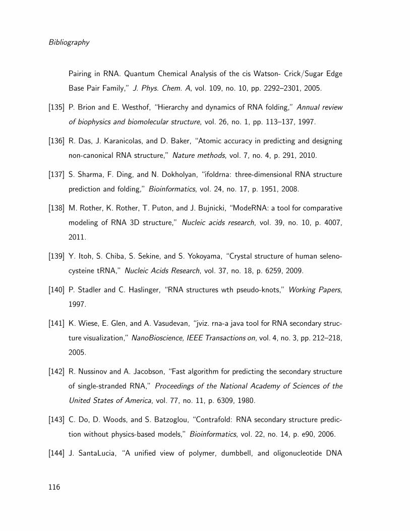
Bibliography
Pairing in RNA. Quantum Chemical Analysis of the cis Watson- Crick/Sugar Edge
Base Pair Family,” J. Phys. Chem. A, vol. 109, no. 10, pp. 2292–2301, 2005.
[135] P. Brion and E. Westhof, “Hierarchy and dynamics of RNA folding,” Annual review
of biophysics and biomolecular structure, vol. 26, no. 1, pp. 113–137, 1997.
[136] R. Das, J. Karanicolas, and D. Baker, “Atomic accuracy in predicting and designing
non-canonical RNA structure,” Nature methods, vol. 7, no. 4, p. 291, 2010.
[137] S. Sharma, F. Ding, and N. Dokholyan, “ifoldrna: three-dimensional RNA structure
prediction and folding,” Bioinformatics, vol. 24, no. 17, p. 1951, 2008.
[138] M. Rother, K. Rother, T. Puton, and J. Bujnicki, “ModeRNA: a tool for comparative
modeling of RNA 3D structure,” Nucleic acids research, vol. 39, no. 10, p. 4007,
2011.
[139] Y. Itoh, S. Chiba, S. Sekine, and S. Yokoyama, “Crystal structure of human seleno-
cysteine tRNA,” Nucleic Acids Research, vol. 37, no. 18, p. 6259, 2009.
[140] P. Stadler and C. Haslinger, “RNA structures wth pseudo-knots,” Working Papers,
1997.
[141] K. Wiese, E. Glen, and A. Vasudevan, “jviz. rna-a java tool for RNA secondary struc-
ture visualization,” NanoBioscience, IEEE Transactions on, vol. 4, no. 3, pp. 212–218,
2005.
[142] R. Nussinov and A. Jacobson, “Fast algorithm for predicting the secondary structure
of single-stranded RNA,” Proceedings of the National Academy of Sciences of the
United States of America, vol. 77, no. 11, p. 6309, 1980.
[143] C. Do, D. Woods, and S. Batzoglou, “Contrafold: RNA secondary structure predic-
tion without physics-based models,” Bioinformatics, vol. 22, no. 14, p. e90, 2006.
[144] J. SantaLucia, “A unified view of polymer, dumbbell, and oligonucleotide DNA
116
Bibliography
nearest-neighbor thermodynamics,” Proceedings of the National Academy of Sci-
ences of the United States of America, vol. 95, no. 4, p. 1460, 1998.
[145] A. Walter, D. Turner, J. Kim, M. Lyttle, P. M
”uller, D. Mathews, and M. Zuker, “Coaxial stacking of helixes enhances binding of
oligoribonucleotides and improves predictions of RNA folding,” Proceedings of the
National Academy of Sciences, vol. 91, no. 20, p. 9218, 1994.
[146] D. Mathews, J. Sabina, M. Zuker, and D. Turner, “Expanded sequence dependence
of thermodynamic parameters improves prediction of RNA secondary structure1,”
Journal of molecular biology, vol. 288, no. 5, pp. 911–940, 1999.
[147] C. Flamm, I. Hofacker, and P. Stadler, “Computational chemistry with rna secondary
structures,” Kemija u industriji, vol. 53, pp. 315–322, 2004.
[148] J. Jaeger, D. Turner, and M. Zuker, “Improved predictions of secondary structures
for RNA,” Proceedings of the National Academy of Sciences of the United States of
America, vol. 86, no. 20, p. 7706, 1989.
[149] M. Zuker and P. Stiegler, “Optimal computer folding of large RNA sequences using
thermodynamics and auxiliary information,” Nucleic acids research, vol. 9, no. 1,
p. 133, 1981.
[150] I. L. Hofacker and P. F. Stadler, RNA Secondary Structures, pp. 439–489. Wiley-VCH
Verlag GmbH, 2008.
[151] M. Zuker, “On finding all suboptimal foldings of an RNA molecule,” Science, vol. 244,
no. 4900, p. 48, 1989.
[152] S. Wuchty, W. Fontana, I. Hofacker, P. Schuster, et al., “Complete suboptimal
folding of RNA and the stability of secondary structures,” Biopolymers, vol. 49,
no. 2, pp. 145–165, 1999.
[153] M. S. Waterman, “Secondary structure of single - stranded nucleic acids,” Studies
117
Bibliography
on foundations and combinatorics, Advances in mathematics supplementary studies,
Academic Press N.Y., vol. 1, pp. 167–212, 1978.
[154] J. McCaskill, “The equilibrium partition function and base pair binding probabilities
for RNA secondary structure,” Biopolymers, vol. 29, no. 6-7, pp. 1105–1119, 1990.
[155] D. Konings and R. Gutell, “A comparison of thermodynamic foldings with compar-
atively derived structures of 16s and 16s-like rRNAs.,” Rna, vol. 1, no. 6, p. 559,
1995.
[156] A. Loria and T. Pan, “Domain structure of the ribozyme from eubacterial ribonuclease
p.,” Rna, vol. 2, no. 6, p. 551, 1996.
[157] H. Mann, Y. Ben-Asouli, A. Schein, S. Moussa, and N. Jarrous, “Eukaryotic RNase
p:: Role of RNA and protein subunits of a primordial catalytic ribonucleoprotein in
RNA-based catalysis,” Molecular cell, vol. 12, no. 4, pp. 925–935, 2003.
[158] D. Staple and S. Butcher, “Pseudoknots: RNA structures with diverse functions,”
PLoS biology, vol. 3, no. 6, p. e213, 2005.
[159] T. Cech, “Conserved sequences and structures of group i introns: building an active
site for RNA catalysis–a review,” Gene, vol. 73, no. 2, pp. 259–271, 1988.
[160] C. Theimer, C. Blois, and J. Feigon, “Structure of the human telomerase RNA
pseudoknot reveals conserved tertiary interactions essential for function,” Molecular
cell, vol. 17, no. 5, pp. 671–682, 2005.
[161] J. Paillart, E. Skripkin, B. Ehresmann, C. Ehresmann, and R. Marquet, “A loop-loop”
kissing” complex is the essential part of the dimer linkage of genomic hiv-1 RNA,”
Proceedings of the National Academy of Sciences of the United States of America,
vol. 93, no. 11, p. 5572, 1996.
[162] J. Reeder and R. Giegerich, “Design, implementation and evaluation of a practi-
118

Bibliography
cal pseudoknot folding algorithm based on thermodynamics,” BMC bioinformatics,
vol. 5, no. 1, p. 104, 2004.
[163] A. Condon, B. Davy, B. Rastegari, S. Zhao, and F. Tarrant, “Classifying RNA pseu-
doknotted structures,” Theoretical Computer Science, vol. 320, no. 1, pp. 35–50,
2004.
[164] C. Reidys, F. Huang, J. Andersen, R. Penner, P. Stadler, and M. Nebel, “Topology
and prediction of RNA pseudoknots,” Bioinformatics, vol. 27, no. 8, p. 1076, 2011.
[165] T. Akutsu, “Dynamic programming algorithms for RNA secondary structure predic-
tion with pseudoknots,” Discrete Applied Mathematics, vol. 104, no. 1-3, pp. 45–62,
2000.
[166] A. Gultyaev, F. Van Batenburg, and C. Pleij, “An approximation of loop free energy
values of RNA h-pseudoknots.,” RNA, vol. 5, no. 5, p. 609, 1999.
[167] M. Andronescu, C. Pop, and A. Condon, “Improved free energy parameters for RNA
pseudoknotted secondary structure prediction,” RNA, vol. 16, no. 1, p. 26, 2010.
[168] J. Bois, S. Venkataraman, H. Choi, A. Spakowitz, Z. Wang, and N. Pierce, “Topolog-
ical constraints in nucleic acid hybridization kinetics,” Nucleic acids research, vol. 33,
no. 13, p. 4090, 2005.
[169] H. Isambert, “The jerky and knotty dynamics of RNA,” Methods, vol. 49, no. 2,
pp. 189–196, 2009.
[170] A. Xayaphoummine, T. Bucher, and H. Isambert, “Kinefold web server for RNA/DNA
folding path and structure prediction including pseudoknots and knots,” Nucleic acids
research, vol. 33, no. suppl 2, p. W605, 2005.
[171] J. Ren, B. Rastegari, A. Condon, and H. Hoos, “HotKnots: heuristic prediction of
RNA secondary structures including pseudoknots,” Rna, vol. 11, no. 10, p. 1494,
2005.
119

Bibliography
[172] J. Sperschneider and A. Datta, “Dotknot: pseudoknot prediction using the probability
dot plot under a refined energy model,” Nucleic Acids Research, vol. 38, no. 7,
p. e103, 2010.
[173] A. Gultyaev, F. Van Batenburg, and C. Pleij, “The computer simulation of RNA
folding pathways using a genetic algorithm,” Journal of Molecular Biology, vol. 250,
no. 1, pp. 37–51, 1995.
[174] L. Cai, R. Malmberg, and Y. Wu, “Stochastic modeling of RNA pseudoknotted
structures: a grammatical approach,” Bioinformatics, vol. 19, no. suppl 1, p. i66,
2003.
[175] S. Cao and S. Chen, “Predicting RNA pseudoknot folding thermodynamics,” Nucleic
acids research, vol. 34, no. 9, p. 2634, 2006.
[176] S. Cao and S. Chen, “Predicting structures and stabilities for H-type pseudoknots
with interhelix loops,” RNA, vol. 15, no. 4, p. 696, 2009.
[177] E. Rivas and S. Eddy, “A dynamic programming algorithm for RNA structure predic-
tion including pseudoknots,” Journal of molecular biology, vol. 285, no. 5, pp. 2053–
2068, 1999.
[178] R. Dirks and N. Pierce, “A partition function algorithm for nucleic acid secondary
structure including pseudoknots,” Journal of Computational Chemistry, vol. 24,
no. 13, pp. 1664–1677, 2003.
[179] W. Beyer, “RNA secondary structure prediction including pseudoknots,” Master The-
sis, 2004.
[180] C. Reidys and P. Stadler, “Combinatorial landscapes,” SIAM review, pp. 3–54, 2002.
[181] B. Hajek, “Cooling schedules for optimal annealing,” Mathematics of operations
research, pp. 311–329, 1988.
120

Bibliography
[182] M. Wolfinger, W. Svrcek-Seiler, C. Flamm, I. Hofacker, and P. Stadler, “Efficient
computation of RNA folding dynamics,” Journal of Physics A: Mathematical and
General, vol. 37, p. 4731, 2004.
[183] C. Flamm, W. Fontana, I. Hofacker, and P. Schuster, “RNA folding at elementary
step resolution.,” Rna, vol. 6, no. 3, p. 325, 2000.
[184] M. Wolfinger, “Landscapes of biopolymers,” PHD Thesis, 2004.
[185] M. Tacker, W. Fontana, P. Stadler, and P. Schuster, “Statistics of RNA melting
kinetics,” European biophysics journal, vol. 23, no. 1, pp. 29–38, 1994.
[186] M. Wolfinger, “The energy landscape of RNA folding,” Diplomarbeit, 2001.
[187] J. Manuch, C. Thachuk, L. Stacho, and A. Condon, “NP-completeness of the energy
barrier problem without pseudoknots and temporary arcs,” Natural Computing, pp. 1–
15, 2011.
[188] S. Morgan and P. Higgs, “Barrier heights between ground states in a model of
RNA secondary structure,” Journal of Physics A: Mathematical and General, vol. 31,
p. 3153, 1998.
[189] C. Flamm, I. Hofacker, S. Maurer-Stroh, P. Stadler, and M. Zehl, “Design of multi-
stable RNA molecules.,” Rna, vol. 7, no. 2, p. 254, 2001.
[190] I. Dotu, W. Lorenz, P. Van Hentenryck, and P. Clote, “Computing folding pathways
between RNA secondary structures,” Nucleic acids research, vol. 38, no. 5, p. 1711,
2010.
[191] M. Andronescu, V. Bereg, H. Hoos, and A. Condon, “RNA STRAND: the RNA
secondary structure and statistical analysis database,” BMC bioinformatics, vol. 9,
no. 1, p. 340, 2008.
[192] M. Rosenblad, J. Gorodkin, B. Knudsen, C. Zwieb, and T. Samuelsson, “SRPDB:
121

Bibliography
Signal recognition particle database,” Nucleic acids research, vol. 31, no. 1, p. 363,
2003.
122

Curriculum Vitae
Stefan Badelt
March 2, 1985, Vienna, Austria
http://www.tbi.univie.ac.at/~stef
Educational Background
2004 – Studies in Molecular Biology, University of Vienna
Diploma Thesis with Prof. Ivo Hofacker: Design of artificial RNA2003 – 2004 Military Service
1995 – 2003 Secondary School (Albertus Magnus School, Vienna)
Professional Experience
2009/05 – Diploma Thesis – Bioinformatics
Design of artificial RNA
Institute for Theoretical Chemistry, Vienna, Austria
(Theoretical Biochemistry Group)
2008/07 – 2008/09 Rotation – Molecular Medicine
Chromosome degradation in apoptotic cells
Max Planck Institute for Molecular Genetics, Berlin, Germany
(Group Ullmann – Molecular Cytogenetics)
2008/03 – 2008/04 Rotation – Immunology
Interaction of Stat1-GRDBD-Stat1 and GRE
Max F. Perutz Laboratories, Vienna, Austria
(Group Kovarik – Infection Biology)
2006/07 – 2009/03 Technician – plasmid library administration, genotyping
Max F. Perutz Laboratories, Vienna, Austria
(Group Kovarik – Infection Biology)
Skills
• Languages: German (native), English, Perl, C, Bash, Latex, R, HTML
• Lab-Techniques: PCR, Real Time PCR, Tissue Culture work (including Nucleofec-
tion), Immunfluorescence, Immunoprecipitation, Nuclear Extract, Western Blot Anal-
ysis, Electrophoretic Mobility Shift Assay, DNA/RNA Extraction, DNA/RNA Gel
Electrophoresis, Reverse Transcription, Array CGH, Oligoarray, BAC Array, ChIP on
Chip.
Conferences, Talks
• TBI Winterseminar in Bled, Slovenia, Feb 13 - 20, 2011
Title: Energy barriers in pseudoknot conformation space
• Herbstseminar Bioinformatik in Vysoka Lıpa, Czech Republic, Oct 5 - 10, 2010
Title: Design & future aspects of artificial RNA-switches in synthetic biology
• TBI Winterseminar in Bled, Slovenia, Feb 14 - 21, 2010
Title: Design of artificial RNA-switches
Recommended