SESSION 3666
Development of a VRML Application
for Teaching Fluid Mechanics
Sunil Appanaboyina, Kendrick Aung
Department of Mechanical Engineering
Lamar University, Beaumont, TX 77710
Abstract
Fluid mechanics is a core subject for Mechanical, Aerospace, Civil, and Chemical
engineering disciplines. One of the main obstacles in teaching fluid mechanics to undergraduate
students is the lack of visualization tools that enhance and improve learning process of the
students. With the widespread availability of multi-media software and hardware tools,
development and integration of 2- and 3-dimensional visualization tools to the undergraduate
fluid curriculum becomes necessary. This paper discusses the development of a Virtual Reality
Modeling Language (VRML) application to be used in an undergraduate fluid mechanics course
at Lamar University. Simple fluid flow problems such as fully developed flow in a pipe are
solved by an application written in Java programming language. The solutions obtained are
displayed in a VRML application that also provides user interaction. Users can change certain
parameters of each problem within a given range, and the VRML application provides the
solution of the problem with new parameters.
Nomenclature
H Half of the distance between plates (m)
L Length of pipe (m)
R0 Radius of pipe (m)
R1 Radius of imaginary pipe (m)
T Time (s)
T0 Temperature of bottom plate or wall of pipe (K)
T1 Temperature of top plate or center of pipe (K)
U Velocity along x-axis (m/s)
U1 Velocity of top plate (m/s)
U2 Velocity of bottom plate (m/s)
Greek letters
o Dynamic viscosity (kg/ms)
m Thermal conductivity (W/mK)
Proceedings of the 2004 American Society for Engineering Education Annual Conference & Exposition
CopyrightÀ 2004, American Society for Engineering Education
Page 9.446.1

p Kinematic viscosity (m2/s)
v Shear stress (N/m2)
f Shear layer stress (N/m2)
Subscripts
0 final or minimum value
1 maximum value
2 fixed
Introduction
Everyday, engineering applications involving fluid flows are encountered by engineers of
many disciplines. As a result, fluid courses form a critical part of the undergraduate core courses
in the mechanical, civil, chemical, aerospace, environmental, petroleum, and biomedical
engineering curricula. Understanding fundamental principles of fluid flow and applying these
principles to engineering applications are problematic for undergraduate engineering students for
the following reasons: the subject involves advanced mathematics topics such as ordinary and
partial differential equations and vector and tensor calculus. Solutions of fluid flow depend on
many parameters, length and time scales, and the solutions are generally obtained by
sophisticated experiments and computations that are difficult to explain. However, when the
result of a fluid flow simulation is presented as a visualization of the calculated flow field, it
becomes a powerful educational tool, giving students an idea of how the fluid behaves under
many different conditions.
Although many Computational Fluid Dynamics (CFD) software packages such as CFX
and Fluent are available in the market, their availability to undergraduate engineering curriculum
has been limited due to the following reasons1:
‚" The software is targeted towards industrial users and the cost tends to be high
‚" The users must have access to powerful, high speed computers to do the analysis
‚" It takes a very long time to get used to the software, i.e. the learning curve is steep
As the technology changes rapidly, the importance of educating and training students in
fluid mechanics becomes more critical. Conventional teaching methods fall short of conveying
the complex ideas needed to be mastered by students. There is a range of problems in this
method of instruction and some of them experienced are2:
‚" Lack of teaching aids to explain the principles used in fluid mechanics
‚" Shortage of time to teach in details
‚" Inadequate visual learning environment
‚" High student to teacher ratio due to increasing number of students
‚" Inability to make the course interesting
‚" Difficulty in explaining students the link between theory and application of fluid
mechanics
‚" Inability to include students who are unable to attend classes
Proceedings of the 2004 American Society for Engineering Education Annual Conference & Exposition
CopyrightÀ 2004, American Society for Engineering Education
Page 9.446.2
Therefore, a variety of learning tools such as interactive texts, multimedia videos and
CD-ROMs, computational and experimental tools, has been developed and used by many
educators teaching fluid and thermodynamics courses in order to improve the learning process of
students1, 3, 4, 5
. Moreover, with the advancements in information technology over the last few
years, conventional teaching methods of having an individual lecture to a group have been
supplemented, and in some cases, replaced by the rapid development and implementation of new
distance learning methods. The development of the Internet, specifically World Wide Web
(WWW), has led to unprecedented growth over the last decade in access to information. It offers
many advantages: ease of use, quick access, low cost, available without the limitation of time or
location, computer platform independent, and flexible in allowing students to control their
learning pace. With the advent of JAVA programming language, which offers features such as
platform independence, engineering applications can be easily developed for the web.
One example is CFDnet1 that provides users with interactive Internet-based access to
powerful server-side meshing, solving, and solution visualization routines for solving practical
engineering problems in fluid flow. Registered users access CFDnet through their web browsers
using a Java user interface. No software downloads or plug-ins are required. It is used in the
undergraduate and graduate teaching of fluid mechanics, and can be used to obtain qualitative
solutions to simple fluid mechanics problems. The driving force behind it is the creation of CFD
software that is readily accessible and simple to use. This allows students, scientists, and
engineers to learn some of the jargon, as well as the basic principles, behind a CFD solution.
When used in conjunction with a fluid mechanics course, it can be used to teach some of the
fundamentals of fluid flow analysis, and 'replace' some of the laboratory experiments used to
teach these principles.
Similar examples include CALF (Computer Aided Learning in Fluid Dynamics)
3, the
NTNU Virtual Physics Laboratory6, Virtual Laboratory
7, and Java Virtual Wind Tunnel
5. CALF
(Computer Aided Learning in Fluid Dynamics) is an interactive web-based course developed at
the Universities of Glasgow and Paisley. It gives an introduction to CFD and covers subjects like
CFD illustrations, turbulence modeling, parallel computing, and grid generation. The NTNU
Virtual Physics Laboratory, a web site developed by Professor Fu-Kwun Hwang, Department of
Physics, National Taiwan Normal University, lists applets for various topics in physics-
mechanics, dynamics, waves, thermodynamics, electromagnetics, light/optics etc. Virtual
Laboratory at John Hopkins University lists a collection of online experiments to enable students
to learn more about experimentation, problem solving, data gathering, and scientific
interpretation. The Java Virtual Wind Tunnel at MIT is an applet which uses computational fluid
dynamics (CFD) methods to simulate the flow of air over a two dimensional object. The applet
solves the equations of motion (the Euler equations) in real time and the simulation provides
more information about the flow than one could easily access in any real wind tunnel. The
Virtual Laboratory8, Department of Physics, University of Oregon, has an interesting collection
of Java applets for use in physics, astronomy, or engineering science courses. It also offers Java
based tools to assist students in making graphs, figures, spreadsheets, etc.
However, these websites are mostly 2-dimensional based websites and do not involve
much interaction. If the fluid mechanics theories are exemplified in a virtual reality environment,
conceptual understanding of the students will be much more enhanced. Important advantages of
virtual reality environment over other computer based design tools are that it enables the user to
interact with the simulation to conceptualize relations that are not apparent from a less dynamic
representation, and to visualize the models that are difficult to understand in other ways.
Proceedings of the 2004 American Society for Engineering Education Annual Conference & Exposition
CopyrightÀ 2004, American Society for Engineering Education
Page 9.446.3

Objectives of the Study
The main objectives of the present work are
(a) To develop a 3-D web-based VRML module for teaching fluid mechanics
(b) To enhance learning process of students by providing an easy, interactive, and graphic
learning tool
(c) To provide educators and students free access to the module
Methodology
Three modules have been developed to illustrate 3-D web-based VRML applications.
These modules use tools such as VRML (Virtual Reality Modeling Language) and JAVA for
interactivity and full 3-D visualization. A virtual environment is a place where a 3D model
exists, that is viewed over the internet using a browser with a VRML plug-in. The Internet has
given rise to a myriad of new technologies and standards. One of the most promising for
engineering has been the Virtual Reality Modeling Language (VRML), which was developed
solely for viewing 3D graphics on the Web. It all started at the “Birds of a feather” sessions
organized by Mark Pesce and Tony Parisi at the 1994 World Wide Web and SIGGRAPH
conferences where many felt the need of a 3D graphics file format that followed a similar model
to HTML, platform-independent, text based scene description language9. The first version of
VRML (VRML 1.0) was developed and available on the Web in 1995. Although it was very
successful as a file format for 3D objects, there was nothing interesting about it, it had two major
limitations: lack of support for dynamic scene animation, and no traditional programming
language constructs. After redefining the language and tackling these issues VRML 2.0 followed
in 1996. This allowed objects to move in the world and allowed the user to interact with them.
This version became an international standard (ISO/IEC 14772) in 1997 under the name
VRML97. This study uses VRML 2.0. At present the Web3D Consortium, the organization
responsible for the creation of open standards for Web3D, is working on X3D (Extensible 3D) as
the successor of VRML 2.0.
The VRML file serves as a blueprint for building the virtual world. It is nothing but a
textual description of the VRML world, it specifies and organizes the structure of the VRML
world. It can be created with any text editor or word processor. VRML files are generally
referred to as worlds and end with an extension .wrl. When a browser reads a VRML file, it
builds the world described in the file and displays it as one moves around the browser. These
files may also contain references to files in many other standard formats like JPEG, PNG, GIF,
and MPEG. WAV and MIDI files may be used to specify sound. Files containing Java or
JavaScript code may be referenced and used to implement programmed behavior for the objects
in the VRML world. VRML files contain four main types of components:
‚" VRML header
‚" Prototypes
‚" Shapes, interpolators, sensors and scripts
‚" Routes
Proceedings of the 2004 American Society for Engineering Education Annual Conference & Exposition
CopyrightÀ 2004, American Society for Engineering Education
Page 9.446.4

In addition to the above components, a VRML file also contains comments, nodes, fields, and
field values. To present 3D VRML worlds, the browser needs special helper applications called
plug-ins. Plug-ins are programs that enable the viewing of non-HTML content in the browser. To
view VRML files, a VRML helper application or a plug-in is needed. For this study, a special
kind of plug-in (ParallelGraphic’s Cortona) was used to view the VRML files.
The programming language used to control the VRML file and perform the calculations
requires seamless integration with the Internet and the web browser. These requirements are
satisfied by the Java programming language developed by the Sun Microsystems. Java has
become very popular because of the many features designed to make it operate on the Internet.
With this language one can “ write once and run anywhere” 10
. Developers can write full-fledged
applications in Java, whose architecture is much like C and C++. It is freely available from the
Sun Microsystems website (http://java.sun.com/). Java can be used to create two types of
programs: applications and applets. An application is a program that runs on the computer, under
the operating system of that computer. An application created using Java is more or less like C or
C++. Java’s ability to create applets is what makes it more important. An applet is an application
designed to be transmitted over the Internet and executed by a Java-compatible Web browser. An
applet is a tiny Java program; dynamically downloaded across the network, just like an image,
sound file or video clip. In other words, an applet is an intelligent program that can react to user
input and dynamically change. The interaction between Java and VRML can be described as
shown in Fig. 1.
Fig. 1 Interaction between Java and VRML (Source: JAVA for 3D and VRML Worlds)
The Modules
Proceedings of the 2004 American Society for Engineering Education Annual Conference & Exposition
CopyrightÀ 2004, American Society for Engineering Education
Page 9.446.5
This section gives the detailed description of the three modules for solving Couette,
Hagen-Poiseuille, and Rayleigh flows.
Couette Flow
The flow was named in the honor of M. Couette11
who performed experiments on the
flow between a fixed and a moving concentric cylinders. Couette flow involves the laminar flow
of an incompressible fluid of constant viscosity between parallel plates, where the bottom plate is
fixed and the top plate travels with a particular velocity. If the fluid flows due to a moving
surface and a pressure gradient, it is called Couette-Poiseuille flow. This flow finds its practical
application in viscous screw pumps and fluid driven motors. Two cases are considered, one
without pressure gradient (plane Couette flow) the other with pressure gradient (generalized
plane Couette flow). Results are also presented for the temperatures calculated between the two
plates in a plane Couette flow.
The flow considers both conservation of momentum and energy equations. In order to
simplify these equations the fluid is assumed to be incompressible, i.e. the density of the fluid is
constant. Furthermore, it is also assumed that the coefficients of viscosity and of heat conduction
of the fluid are constant. The program allows the choice of fluids with different properties: air,
water, glycerin, SAE30 oil or mercury. The user needs to provide necessary parameters such as
velocity of the top plate, type of fluid, gap between the plates, and the pressure gradient. The
results for this flow consist of a velocity profile and a temperature profile. With the velocity
profile, results such as shear stress and the position of maximum velocity are also shown. In case
of the temperature profile the user enters the temperatures of the top and bottom plates.
Eq. 1 gives the solution for the velocity profile of the Couette flow
22
12
2121
2
22 UU
h
yUU
h
y
dx
dphu
--
/-ÕÕ
Ö
ÔÄÄÅ
Ã//?
o (1)
where is the velocity between the plates at a particular , is the half distance between the
plates, velocity of the top plate, U velocity of the bottom plate and
u
U
y h
1 2dx
dp is the pressure
difference. Shear stress is calculated using the following equation
??h
U
2
ov constant (2)
and Eq. 3 determines the position of the maximum velocity.
* +
hP
Py
2
1-? (3)
where ÕÖ
ÔÄÅ
Ã/?
dx
dp
U
hP
o2
2
. In the case of no pressure gradient, 0?dx
dp, and a stationary bottom
plate, U , the velocity profile is given by 02 ?
Proceedings of the 2004 American Society for Engineering Education Annual Conference & Exposition
CopyrightÀ 2004, American Society for Engineering Education
Page 9.446.6

ÕÖ
ÔÄÅ
à -?h
yUu 1
2 (4)
In this case, the velocity distribution is linear between the two plates. In the case with pressure
gradient, 0@dx
dp, but a stationary bottom plate, 02 ?U , the velocity profile is given by
ÕÖ
ÔÄÅ
à --ÕÕÖ
ÔÄÄÅ
Ã//?
h
yU
h
y
dx
dphu 1
21
2
1
2
22
o (5)
The velocity distribution is parabolic between the two plates. The VRML model for the couette
flow starts with the screen showing two parallel plates and a Java frame window to accept input
from the user. The frame window asks for the following inputs: top plate velocity in m/s, type of
fluid, which the user selects from a list, gap between plates in m and the pressure difference in
Pa. The opening screen shot of the Couette flow problem is shown in Fig. 2.
Fig. 2 An Opening Screen Shot of the Couette Flow Problem (Velocity)
The user enters the values and clicks the draw button. In the case of plane couette flow,
the pressure difference is zero. The result is shown with the layer of fluid with maximum
velocity as a row of arrows in red color, the color changes till blue, which represents the
minimum velocity. The magnitude of the velocity of the layer of fluid is known from the velocity
legend. The profile obtained is of linear in nature as indicated by Eq. 4.
Proceedings of the 2004 American Society for Engineering Education Annual Conference & Exposition
CopyrightÀ 2004, American Society for Engineering Education
Page 9.446.7
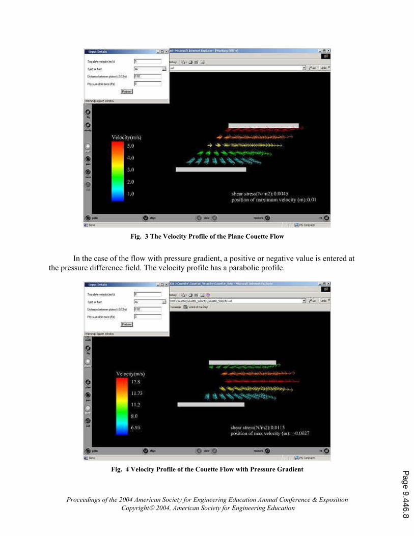
Fig. 3 The Velocity Profile of the Plane Couette Flow
In the case of the flow with pressure gradient, a positive or negative value is entered at
the pressure difference field. The velocity profile has a parabolic profile.
Fig. 4 Velocity Profile of the Couette Flow with Pressure Gradient
Proceedings of the 2004 American Society for Engineering Education Annual Conference & Exposition
CopyrightÀ 2004, American Society for Engineering Education
Page 9.446.8
The solution of the temperature profile for a plane couette flow involving a laminar flow
of an incompressible fluid between two parallel plates is given by
ÕÕÖ
ÔÄÄÅ
Ã/-ÙÚ
×ÈÉ
Ç /-
-?
2
22
0101 1822 h
y
k
U
h
yTTTTT
o (6)
The term inside the square brackets represents the straight-line distribution, which would arise
due to pure conduction in the fluid. The second (parabolic) term is the temperature rise due to
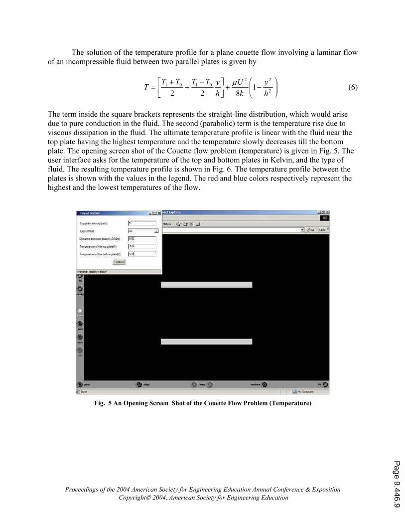
viscous dissipation in the fluid. The ultimate temperature profile is linear with the fluid near the
top plate having the highest temperature and the temperature slowly decreases till the bottom
plate. The opening screen shot of the Couette flow problem (temperature) is given in Fig. 5. The
user interface asks for the temperature of the top and bottom plates in Kelvin, and the type of
fluid. The resulting temperature profile is shown in Fig. 6. The temperature profile between the
plates is shown with the values in the legend. The red and blue colors respectively represent the
highest and the lowest temperatures of the flow.
Fig. 5 An Opening Screen Shot of the Couette Flow Problem (Temperature)
Proceedings of the 2004 American Society for Engineering Education Annual Conference & Exposition
CopyrightÀ 2004, American Society for Engineering Education
Page 9.446.9
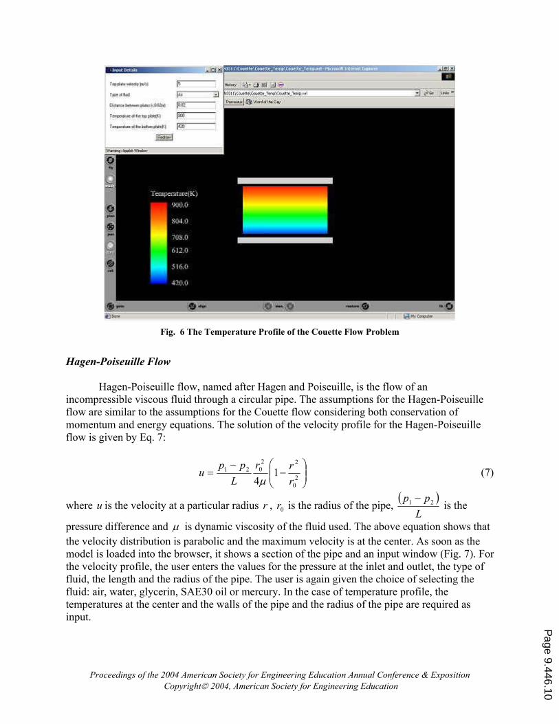
Fig. 6 The Temperature Profile of the Couette Flow Problem
Hagen-Poiseuille Flow
Hagen-Poiseuille flow, named after Hagen and Poiseuille, is the flow of an
incompressible viscous fluid through a circular pipe. The assumptions for the Hagen-Poiseuille
flow are similar to the assumptions for the Couette flow considering both conservation of
momentum and energy equations. The solution of the velocity profile for the Hagen-Poiseuille
flow is given by Eq. 7:
ÕÕÖ
ÔÄÄÅ
Ã/
/?
2
0
22
021 14 r
rr
L
ppu
o (7)
where u is the velocity at a particular radius r , is the radius of the pipe, 0r* +
L
pp 21 / is the
pressure difference and o is dynamic viscosity of the fluid used. The above equation shows that
the velocity distribution is parabolic and the maximum velocity is at the center. As soon as the
model is loaded into the browser, it shows a section of the pipe and an input window (Fig. 7). For
the velocity profile, the user enters the values for the pressure at the inlet and outlet, the type of
fluid, the length and the radius of the pipe. The user is again given the choice of selecting the
fluid: air, water, glycerin, SAE30 oil or mercury. In the case of temperature profile, the
temperatures at the center and the walls of the pipe and the radius of the pipe are required as
input.
Proceedings of the 2004 American Society for Engineering Education Annual Conference & Exposition
CopyrightÀ 2004, American Society for Engineering Education
Page 9.446.10
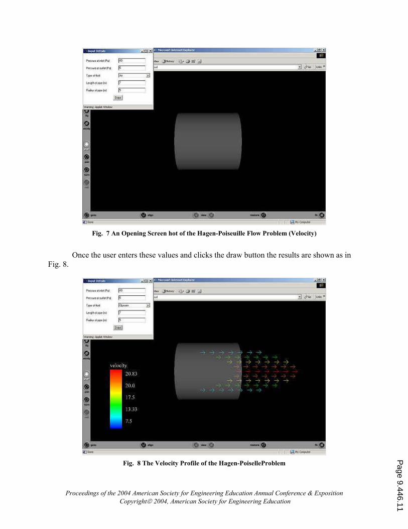
Fig. 7 An Opening Screen hot of the Hagen-Poiseuille Flow Problem (Velocity)
Once the user enters these values and clicks the draw button the results are shown as in
Fig. 8.
Fig. 8 The Velocity Profile of the Hagen-PoiselleProblem
Proceedings of the 2004 American Society for Engineering Education Annual Conference & Exposition
CopyrightÀ 2004, American Society for Engineering Education
Page 9.446.11
The velocity profile is of parabolic shape with the maximum velocity at the center. The
result is shown with the layer of fluid with maximum velocity as a row of arrows in red color, the
color changes till blue, which represents the minimum velocity. The velocity legend gives the
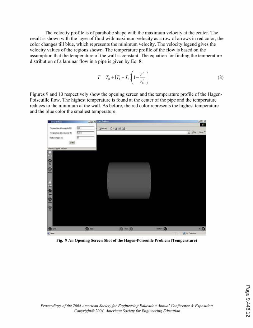
velocity values of the regions shown. The temperature profile of the flow is based on the
assumption that the temperature of the wall is constant. The equation for finding the temperature
distribution of a laminar flow in a pipe is given by Eq. 8:
* + ÕÕÖ
ÔÄÄÅ
Ã//-?
4
0
4
010 1r
rTTTT (8)
Figures 9 and 10 respectively show the opening screen and the temperature profile of the Hagen-
Poiseuille flow. The highest temperature is found at the center of the pipe and the temperature
reduces to the minimum at the wall. As before, the red color represents the highest temperature
and the blue color the smallest temperature.
Fig. 9 An Opening Screen Shot of the Hagen-Poiseuille Problem (Temperature)
Proceedings of the 2004 American Society for Engineering Education Annual Conference & Exposition
CopyrightÀ 2004, American Society for Engineering Education
Page 9.446.12

Fig. 10 The Temperature Profile of the Hagen-Poiselle Problem
Raleigh Flow
Investigated by Lord Rayleigh, this problem deals with the solution of the impulsive
motion of an infinite plate12
. Raleigh problem deals with the movement of an incompressible
viscous fluid over a suddenly moving flat plate with a particular velocity. This problem also
solves the conservation of energy and momentum equations. Assumptions are made that the fluid
is incompressible, i.e. the density is constant and that the coefficients of viscosity and heat
conduction of the fluid are constant. This problem involves the sudden movement of a plate in its
own plane with a constant velocity U. Equation 9 below gives the solution of the Raleigh flow
problem:
))(1( jerfUu /? (9)
where vt
y
2?j , is the distance in the y-direction, y p is kinematic viscosity and t is the
time. The shear layer thickness is calculated using Eq. 10.
vt64.3?f (10)
A screen shot of the Raleigh problem interface is given in Fig. 11. The model is a flat
plate with a frame to input the plate velocity in m/s and the type of fluid used. The user is again
given the choice of selecting the fluid: air, water, glycerin, SAE30 oil or mercury.
Proceedings of the 2004 American Society for Engineering Education Annual Conference & Exposition
CopyrightÀ 2004, American Society for Engineering Education
Page 9.446.13
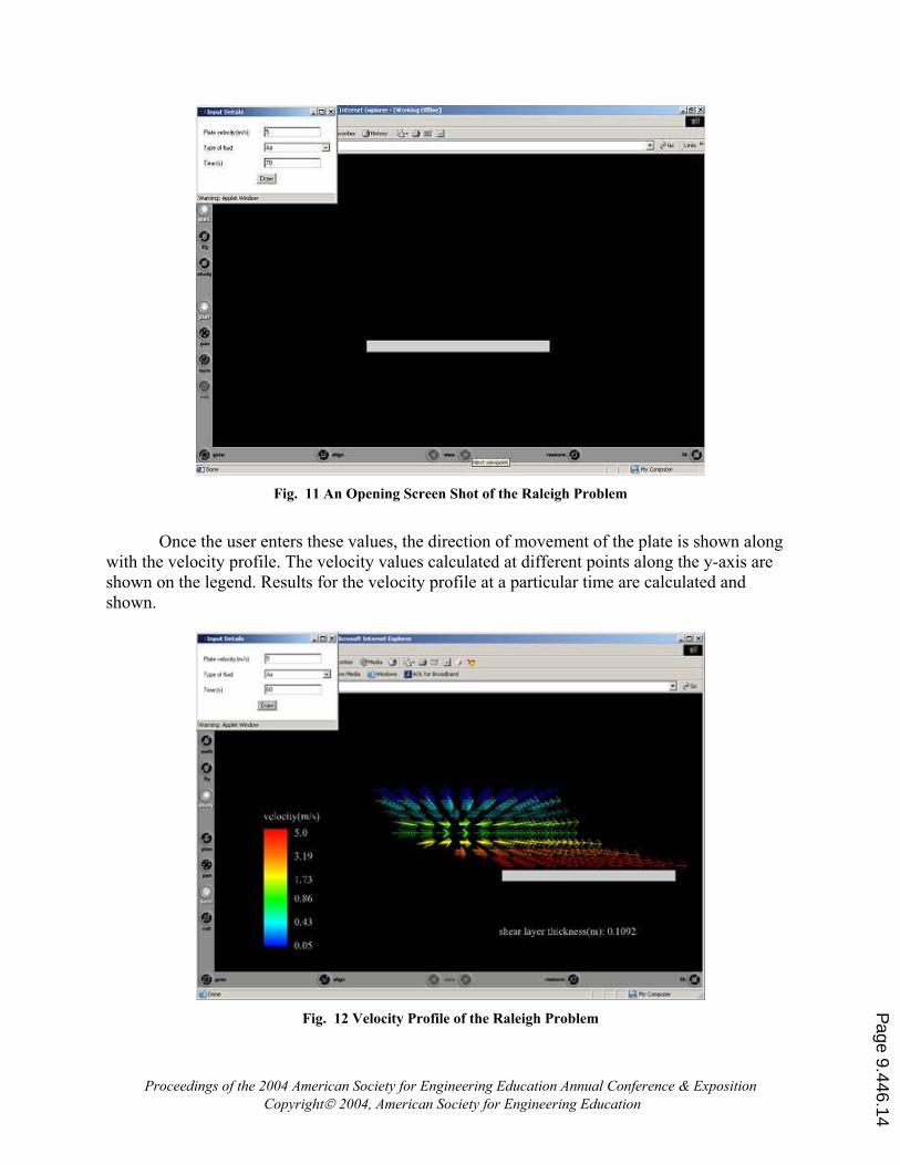
Fig. 11 An Opening Screen Shot of the Raleigh Problem
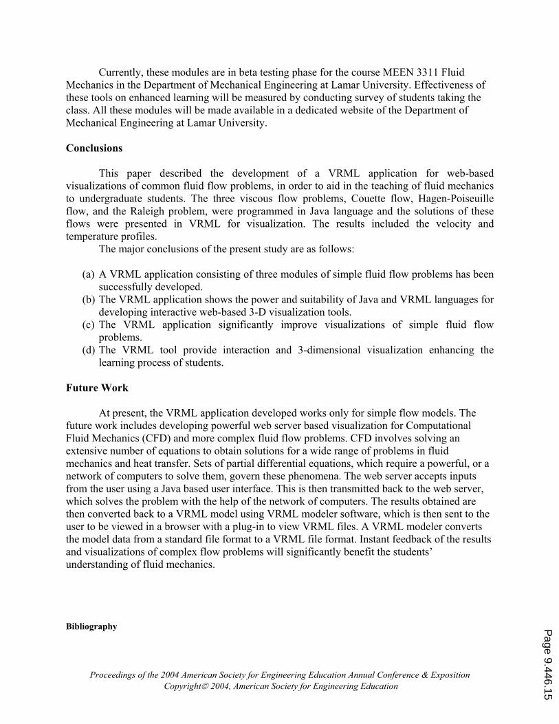
Once the user enters these values, the direction of movement of the plate is shown along
with the velocity profile. The velocity values calculated at different points along the y-axis are
shown on the legend. Results for the velocity profile at a particular time are calculated and
shown.
Fig. 12 Velocity Profile of the Raleigh Problem
Proceedings of the 2004 American Society for Engineering Education Annual Conference & Exposition
CopyrightÀ 2004, American Society for Engineering Education
Page 9.446.14
Currently, these modules are in beta testing phase for the course MEEN 3311 Fluid
Mechanics in the Department of Mechanical Engineering at Lamar University. Effectiveness of
these tools on enhanced learning will be measured by conducting survey of students taking the
class. All these modules will be made available in a dedicated website of the Department of
Mechanical Engineering at Lamar University.
Conclusions
This paper described the development of a VRML application for web-based
visualizations of common fluid flow problems, in order to aid in the teaching of fluid mechanics
to undergraduate students. The three viscous flow problems, Couette flow, Hagen-Poiseuille
flow, and the Raleigh problem, were programmed in Java language and the solutions of these
flows were presented in VRML for visualization. The results included the velocity and
temperature profiles.
The major conclusions of the present study are as follows:
(a) A VRML application consisting of three modules of simple fluid flow problems has been
successfully developed.
(b) The VRML application shows the power and suitability of Java and VRML languages for
developing interactive web-based 3-D visualization tools.
(c) The VRML application significantly improve visualizations of simple fluid flow
problems.
(d) The VRML tool provide interaction and 3-dimensional visualization enhancing the
learning process of students.
Future Work
At present, the VRML application developed works only for simple flow models. The
future work includes developing powerful web server based visualization for Computational
Fluid Mechanics (CFD) and more complex fluid flow problems. CFD involves solving an
extensive number of equations to obtain solutions for a wide range of problems in fluid
mechanics and heat transfer. Sets of partial differential equations, which require a powerful, or a
network of computers to solve them, govern these phenomena. The web server accepts inputs
from the user using a Java based user interface. This is then transmitted back to the web server,
which solves the problem with the help of the network of computers. The results obtained are
then converted back to a VRML model using VRML modeler software, which is then sent to the
user to be viewed in a browser with a plug-in to view VRML files. A VRML modeler converts
the model data from a standard file format to a VRML file format. Instant feedback of the results
and visualizations of complex flow problems will significantly benefit the students’
understanding of fluid mechanics.
Bibliography
Proceedings of the 2004 American Society for Engineering Education Annual Conference & Exposition
CopyrightÀ 2004, American Society for Engineering Education
Page 9.446.15

Proceedings of the 2004 American Society for Engineering Education Annual Conference & Exposition
CopyrightÀ 2004, American Society for Engineering Education
1. Ham, F.E., Militzer, J., & Bemfica, A. (1998). CFDnet: Computational Fluid Dynamics on the Internet.
Retrieved November 12, 2002, from http://www.cfdnet.com.
2. Haque, M.E. (2001). Web-based visualization techniques for structural design education. Retrieved August
23, 2002, from http://www.asee.org/conferences/search/01143_2001.pdf.
3. CALF. (1996). Retrieved July 2, 2003, from University of Glasgow and University of Paisley, United
Kingdom, Web site: http://cvu.strath.ac.uk/courseware/calf/CALF/index/web_calf.html.
4. TEST. (2001). Retrieved October 12, 2002, from San Diego State University, San Diego, Web site:
http://kahuna.sdsu.edu/testcenter/.
5. The Java virtual wind tunnel. (1996). Retrieved July 2,2003, from Massachusetts Institute of Technology,
Cambridge, Web site: http://raphael.mit.edu/Java/.
6. Virtual physics laboratory. (2003). Retrieved July 2, 2003, from National Taiwan Normal University,
Taiwan, Web site: http://www.phy.ntnu.edu.tw/java/index.html.
7. Virtual lab. (2000). Retrieved July 2, 2003, from The Johns Hopkins University, Baltimore, Web site:
http://www.jhu.edu/~virtlab/virtlab.html.
8. Virtual laboratory. (2003). Retrieved July2, 2003, from University of Oregon, Eugene, Web site:
http://jersey.uoregon.edu/vlab/.
9. Brutzman, D. (1998). The virtual reality modeling language and Java. Communications of the ACM, 41(6),
57-64.
10. Lea, R., Matsuda, K., & Miyashita, K. (1996). Java for 3D and VRML worlds (1st ed.). Indianapolis, IN:
New Riders.
11. White, F.M. (1991). Viscous fluid flow (2nd ed.). New York: McGraw Hill.
12. Pai, S. (1956). Viscous flow theory I-laminar flow (1st ed.). New York: D. Van Nostrand.
Biography
SUNIL APPANABOYINA is a pre-candidate for the Doctor of Engineering in the Department of Mechanical
Engineering at James Mason University. This paper was his Masters thesis work under the supervision of Dr.
Kendrick Aung (Co-author of this paper) when he was with the Department of Mechanical Engineering at Lamar
University.
KENDRICK AUNG is an assistant professor in the Department of Mechanical Engineering at Lamar University. He
received his Ph.D. degree in Aerospace Engineering from University of Michigan in 1996. He is an active member
of ASEE, ASME, AIAA and Combustion Institute. He has published over 50 technical papers and presented many
papers at national and international conferences.
Page 9.446.16
Recommended