The Pennsylvania State University
The Graduate School
College of Engineering
DEVELOPMENT OF A CORRELATION FOR NUCLEATE BOILING
HEAT FLUX ON A HEMISPHERICAL DOWNWARD FACING SURFACE
A Thesis in
Mechanical Engineering
by
Michael P Riley
© 2012 Michael P. Riley
Submitted in Partial Fulfillment
of the Requirements
for the Degree of
Master of Science
May 2012

The thesis of Michael P. Riley was reviewed and approved* by the following:
Fan-Bill Cheung
Professor of Mechanical and Nuclear Engineering
Thesis Adviser
Savas Yavuzkurt
Professor of Mechanical Engineering
Karen A. Thole
Professor of Mechanical Engineering
Head of the Department of Mechanical Engineering
*Signatures are on file in the Graduate School.
iii
ABSTRACT
A new physics-based heat transfer correlation has been developed that can be
used to predict the local variation of the nucleate boiling heat flux on a downward facing
heating surface. It is widely known that the heat transfer mechanism of nucleate boiling
involves the growth and departure of vapor bubbles on a heated surface. When the vapor
bubbles have grown to their mature size, they depart from the heating surface, agitating
the surrounding fluid. This bubble agitation results in strong turbulent mixing of the
fluid. For the case of an upward facing surface, the nucleate boiling heat flux has been
determined using the single-phase turbulent heat transfer correlation. The correlation
relates the Nusselt number to the Reynolds number and Prandtl number. Through the use
of proper velocity and length scales, Rohsenow (1952) developed a correlation to predict
the nucleate boiling heat flux on an upward facing surface. The resulting correlation
relates the nucleate boiling heat flux to the wall superheat and fluid properties and a
correlation coefficient.
For the case of downward facing boiling on a hemispherical surface, however, the
Rohsenow correlation cannot be applied. Due to the surface orientation, buoyancy
effects have a significant impact on the behavior of the flow and heat transfer. The
heating surface causes the fluid in close proximity to increase in temperature, lowering
the density of the fluid. When the liquid begins to vaporize, the density of the resulting
vapor is several orders of magnitude less than the surrounding liquid, resulting in strong
buoyancy forces that entrain the liquid upward. The downward facing surface hinders
this upward motion of vapor bubbles, causing them to have to take an alternative upward
route. If the surface is inclined, the bubbles will flow along the heating surface which
iv
develops into a two-phase boundary layer flow. When the surface is completely
horizontally downward facing, the bubbles cannot flow along the surface, forming a
vapor blanket from which bubbles shear off.
The Rohsenow correlation relates the nucleate boiling heat flux to only wall
superheat and fluid properties. Local variation does not appear in the correlation because
the nucleate boiling heat flux conditions are equivalent at all locations of an upward
facing surface. On a downward facing hemispherical surface, however, local variation
plays a significant role in the nucleate boiling heat flux. At the bottom of the
hemispherical surface, the buoyancy force presses the vapor bubbles against the surface.
As the local coordinate along the surface is increased, the buoyancy forces have an
increasing impact on the flow characteristics and, thus, the heat flux.
The present study has successfully captured the local buoyancy effects and local
variation of the nucleate boiling heat flux on a downward facing surface. The correlation
predicts the nucleate boiling heat flux based on the wall superheat, fluid properties, and,
most importantly, local variation along the heating surface. Similar to the Rohsenow
correlation, the correlation for the present study is derived from a bubble-induced flow
mixing Nusselt number correlation. The length and velocity scales are chosen based on a
scale analysis of the momentum and energy equations for a buoyancy-driven boundary
layer flow. The correlation coefficient is calculated based on the particular flow
geometry under consideration. For this study, the correlation coefficients are calculated
for the AP600 and Korea Next-Generation Reactor (KNGR) nuclear reactors. The new
correlation successfully predicts the nucleate boiling heat flux for a downward facing
surface.
v
TABLE OF CONTENTS
List of Figures .................................................................................................................. vii
List of Tables .................................................................................................................... ix
Nomenclature .....................................................................................................................x
Acknowledgements ........................................................................................................ xiv
1 Introduction .....................................................................................................................1
1.1 Background ................................................................................................................1
1.2 Current Data and Correlations ....................................................................................2
1.3 Motivation for the Present Work ................................................................................5
2 Literature Review ...........................................................................................................6
2.1 Pool Boiling ................................................................................................................6
2.2 Previous Experiments with an Inclined Boiling Surface ...........................................9
2.3 Bubble Dynamics on an Inclined Boiling Surface ...................................................12
2.4 Nucleation Sites and Bubble Growth .......................................................................15
2.5 Nucleate Boiling Heat Flux Correlations .................................................................19
2.6 Flow Boiling .............................................................................................................22
2.7 Saturate Flow Boiling Characteristics in the Nucleate Boiling Regime ..................26
3 Upward Facing Boiling .................................................................................................28
3.1 Extension of Single-Phase to Two-Phase Heat Transfer .........................................28
3.2 Nusselt Number Correlation .....................................................................................29
3.3 Velocity, Length, and Temperature Scales ..............................................................30
4 Downward Facing Boiling – Theoretical Work .........................................................33
4.1 Comparison to Upward Facing Boiling ...................................................................33
4.2 Development of Scales .............................................................................................34
4.3 Development of the Nusselt Number Correlation ....................................................37
vi
5 Downward Facing Boiling – Experimental Work ......................................................40
5.1 Overview of the Test Facility ...................................................................................40
5.2 Experimental Setup ..................................................................................................45
5.3 Experimental Results ................................................................................................47
6 Results and Discussion ..................................................................................................50
6.1 Boiling Heat Transfer from the Bottom Center Region ...........................................50
6.2 Values Chosen for and Physical Implications .....................................................52
6.3 Nucleate Boiling Heat Flux Dependence on and with Value for ...............52
6.4 Correlation Coefficient’s Dependence on .............................................................53
6.5 Comparison of the Proposed Correlation with the Measured Data ..........................55
7 Conclusions and Recommendations ............................................................................62
7.1 Overall Behavior of Buoyancy Driven Convection .................................................62
7.2 Extension of Single-Phase Flow and Heat Transfer to Two-Phase Flow and Heat
Transfer ..........................................................................................................................63
7.3 Range of Validity of the Correlation ........................................................................63
7.4 Recommendations for Future Work .........................................................................64
References .........................................................................................................................65
Appendix A – Scale Analysis of Buoyancy Driven Flow Along a Downward Facing
Surface .............................................................................................................................68
Appendix B – Detailed Derivation of the Downward Facing Boiling Heat Transfer
Correlation........................................................................................................................74
Appendix C – Raw Data for AP600 ...............................................................................76
Appendix D – Raw Data for KNGR ...............................................................................81

vii
LIST OF FIGURES
Fig. 1.1. AP600 Baffle Structure .......................................................................................3
Fig. 1.2. KNGR Baffle Structure ......................................................................................4
Fig. 2.1. Pool Boiling Curve for Water .............................................................................6
Fig. 2.2. Schematic of Transition from Partial to Fully Developed Nucleate Boiling ..8
Fig. 2.3. Vapor Bubble near the Surface during Film Boiling .......................................8
Fig. 2.4. Cross-Sectional View of a Conical Crevice .....................................................16
Fig. 2.5. Bubble Growth Steps ........................................................................................17
Fig. 2.6. Flow Boiling Regimes and Temperature Profile in a Vertical Channel .......23
Fig. 2.7. Horizontal Flow Boiling Regimes ....................................................................25
Fig. 4.1. Schematic of the Downward Facing Surface ..................................................35
Fig. 5.1. Top View of the Water Tank ............................................................................40
Fig 5.2. Front View of the Water Tank ..........................................................................41
Fig 5.3. Side View of the Water Tank ...........................................................................41
Fig. 5.4. Top View of the Cartridge Heater Placement ................................................43
Fig. 5.5. Schematic of the Cartridge Heater Placement ...............................................44
Fig. 5.6. Close-Up of the Upper Cartridge Heater ........................................................44
viii
Fig. 5.7. Schematic of the Power Control System Used to Detect CHF ......................46
Fig. 5.8. AP600 Downward Facing Boiling Data ...........................................................49
Fig. 5.9. KNGR Downward Facing Boiling Data ..........................................................49
Fig. 6.1. Schematic of Two-Phase Boundary Layer ......................................................51
Fig. 6.2. AP600 Correlation Coefficient .........................................................................54
Fig. 6.3. KNGR Correlation Coefficient ........................................................................54
Fig. 6.4. AP600 Heat Flux Data at .....................................................................56
Fig. 6.5. AP600 Heat Flux Data at ...................................................................57
Fig. 6.6. AP600 Heat Flux Data at ...................................................................57
Fig. 6.7. AP600 Heat Flux Data at ...................................................................58
Fig. 6.8. AP600 Heat Flux Data at ...................................................................58
Fig. 6.9. KNGR Heat Flux Data at .....................................................................59
Fig. 6.10. KNGR Heat Flux Data at ................................................................60
Fig. 6.11. KNGR Heat Flux Data at ................................................................60
Fig. 6.12. KNGR Heat Flux Data at ................................................................61
Fig. 6.13. KNGR Heat Flux Data at ................................................................61
ix
LIST OF TABLES
Table C.1: Steady State Saturated Nucleate Boiling Data at the Bottom Center
.............................................................................................................................76
Table C.2: Steady State Saturated Nucleate Boiling Data at ........................77
Table C.3: Steady State Saturated Nucleate Boiling Data at ........................78
Table C.4: Steady State Saturated Nucleate Boiling Data at ........................79
Table C.5: Steady State Saturated Nucleate Boiling Data at ........................80
Table D.1: Steady State Saturated Nucleate Boiling Data at the Bottom Center
.............................................................................................................................81
Table D.2: Steady State Saturated Nucleate Boiling Data at ........................82
Table D.3: Steady State Saturated Nucleate Boiling Data at ........................83
Table D.4: Steady State Saturated Nucleate Boiling Data at ........................84
Table D.5: Steady State Saturated Nucleate Boiling Data at ........................85

x
NOMENCLATURE
Correlation constant
Constant in minimum and maximum crevice size equation
Constant in minimum and maximum crevice size equation
Heat capacity
Surface-fluid constant in Rohsenow (1952) equation
Velocity scale constant
Correction factor
Acceleration due to gravity
Convection heat transfer coefficient
Flow boiling heat transfer coefficient
Nucleate boiling heat transfer coefficient
Latent heat of vaporization
Conduction heat transfer coefficient
Length scale
Mass flow rate
Molecular mass

xi
Exponent (used in multiple contexts)
Nusselt number
Vapor pressure inside bubble
Pressure of liquid surrounding bubble
Critical pressure
Saturation pressure
Prandtl number
Nucleate boiling heat flux
Wall heat flux
Radius of a perfectly spherical bubble
Reynolds number
Minimum radius of a non-spherical vapor bubble (does not apply to conical
crevice)
Maximum radius of a non-spherical vapor bubble (does not apply to conical
crevice)
Radius of bubble and conical cavity
Minimum crevice size for bubble growth
Maximum crevice size for bubble growth

xii
Roughness parameter
Ambient temperature
Saturation temperature
Wall temperature
Velocity
Velocity scale
Greek Symbols
Difference in properties
Wall superheat temperature
Thermal diffusivity
Thermal expansion coefficient
Vapor layer thickness
Angular position on vessel head
Dynamic viscosity
Kinematic viscosity
Density
Surface tension
xiii
Subscripts
Fluid property
Reference value
Vapor property

xiv
ACKNOWLEDGMENTS
First and foremost, I would like to thank God for giving me the strength and
ability to complete this project and earning my Master of Science in Mechanical
Engineering degree and also helping me overcome hardships while making the bright
times brighter.
I also would like to express my gratitude to my advisor, Dr. Fan-Bill Cheung, for
guiding me through this process. His strong belief and investment in me has helped me
to grow both professionally and personally.
It is impossible to express enough gratitude to my parents, Sean and Laura, for
raising me and providing me with the guidance to be a successful person. The same can
be said about my siblings, Sean, Kathleen, and Kevin, who have always stuck with me
throughout my life.
I would like to extend my thanks to Dr. Gita Talmage who has provided me with
valuable guidance throughout my time as a graduate student at Penn State.
I also would like to thank Dr. Savas Yavuzkurt, who provided me with
suggestions to help make this work more complete.
Finally, I would like to thank all of my friends and co-workers as well as the
faculty and staff at Penn State who have made my experiences in graduate school more
enjoyable and fulfilling.
1
1. Introduction
1.1 Background
In an advanced light water reactor (ALWR), the core must be sufficiently cooled.
Insufficient cooling of the core could cause it to melt and relocate downward into the
lower head of the reactor vessel. If this happens, the reactor vessel must be properly
cooled in order to avoid failure of the vessel head. If the vessel can be properly cooled in
the case of such an accident, contamination and failure risks can be minimized.
Under severe accident conditions, the type of heat transfer taking place on the
vessel head may vary significantly. Different heat transfer regimes may be present at
different times, leading to an overall transient heat transfer process on the vessel wall.
Theofanous et al. (1996) stated that the pool of core melt is not well mixed and that its
temperature cannot be described as a single bulk temperature. The pool temperature is
actually very non-uniform.
The melting point of the vessel head is approximately 1400°C, which is much
lower than the freezing temperature of the molten pool of the core melt which is
approximately 2830°C. This difference in melting and freezing temperatures causes the
core melt to form a ceramic crust between itself and the vessel head. Heat is conducted
from the ceramic crust to the vessel head while heat is convected from the core melt to
the ceramic crust. If the heat flux from the crust to the vessel is greater than the heat flux
from the core melt to the crust, the crust will grow. Otherwise, the crust will decay in
thickness.
2
A layer of molten steel (from the vessel head) could form between the ceramic
crust and vessel head, depending on the thermal loading conditions. Whether or not the
vessel head melts is dependent largely on the amount of heat removed from the exterior
surface of the vessel wall. This heat flux is the cooling mechanism for the vessel wall,
which is by the mechanism of downward facing boiling.
1.2 Current Data and Correlations
When it comes to the boiling heat flux, a very important point to consider is the
critical heat flux (CHF) limit. It is at this point that the boiling heat transfer regime
changes very quickly from nucleate boiling to film boiling. At heat flux values above the
CHF point, the temperature of the boiling surface increases very rapidly with small
increases in the heat flux. For safe operating conditions of the reactor vessel, it is
important to remain below the CHF point. Liu (1999) developed a correlation, based on
experimental data, which predicts the temperature at which the CHF occurs.
Previous downward facing boiling work was carried out by Haddad, Cheung, and
Liu (1997). Their experiments involved a downward facing hemispherical surface
submerged in a large pool of water, such that the flow around the hemisphere was
external. The experiments of Liu (1999) involved placing a baffle structure around the
hemisphere so that an internal flow would be induced. Two of the baffle structures under
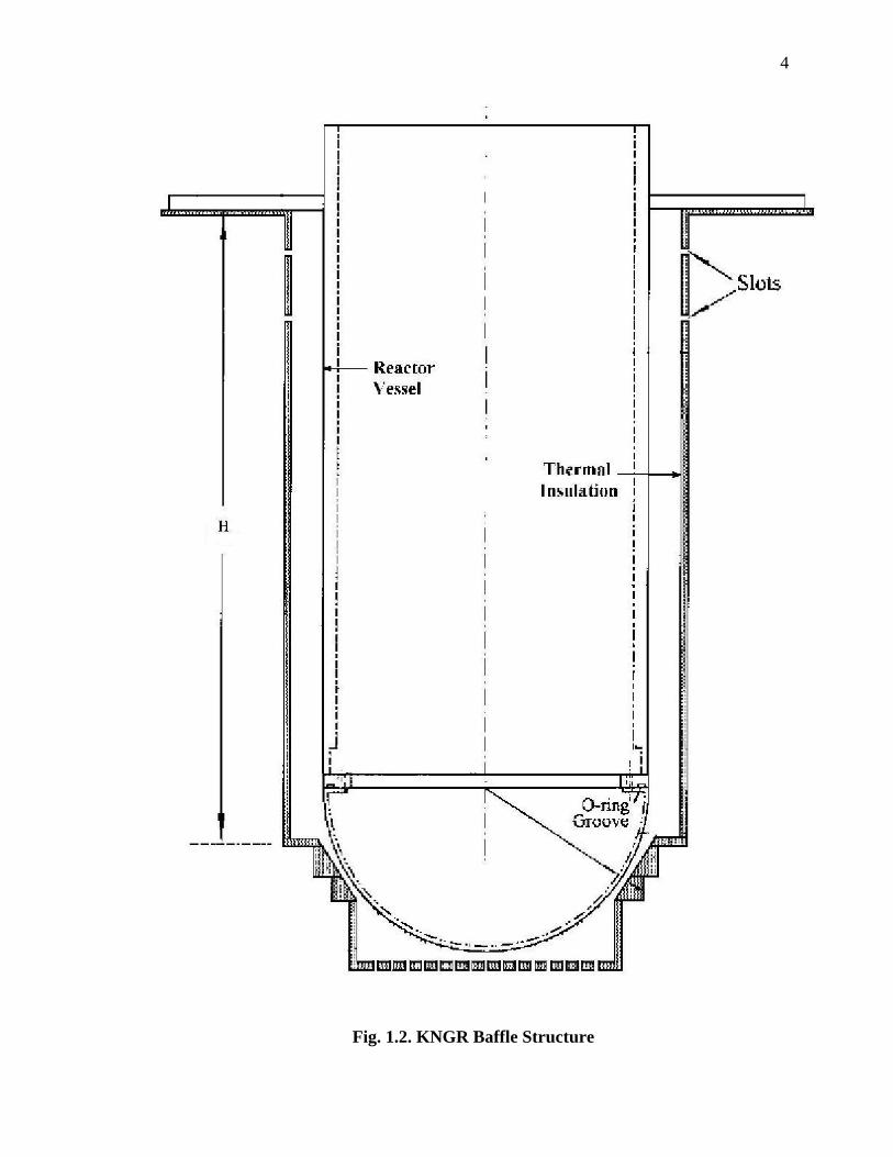
consideration are shown in figures 1.1 and 1.2. Figure 1.1 shows the baffle structure for
the AP600 reactor, whereas figure 1.2 shows the baffle structure for the Korean Next
Generation Reactor (KNGR). Liu discovered that the CHF is significantly increased
when the baffle structure is present, leading to more efficient cooling of the vessel head.
3
Fig. 1.1. AP600 Baffle Structure
4
Fig. 1.2. KNGR Baffle Structure
5
1.3 Motivation for the Present Work
The studies carried out by Haddad, Cheung, and Liu (1997) and of Liu (1999)
focused primarily on predicting the occurrence of the CHF limit for boiling on a
hemispherical downward facing surface. Under coolable operating conditions, however,
the CHF condition is undesirable. Should the CHF point be reached, any slight increase
in the heat flux would cause a very large increase in the vessel wall temperature. In such
case, the core melt would breach through the vessel head, causing a catastrophic accident.
Safe and coolable operating conditions demand that the heat flux be maintained below
the CHF point such that all of the decay energy from the core melt would be removed by
nucleate boiling on the vessel outer surface. Thus far, no correlation or heat transfer
model is available in the literature that can be utilized to predict the local boiling heat
flux for downward facing boiling on the vessel outer surface under nucleate boiling
conditions. In the present study, a physics-based correlation is developed that accurately
predicts the nucleate boiling heat flux for conditions below the CHF point.

6
2. Literature Review
2.1 Pool Boiling
When a liquid is heated to the point where it vaporizes, the liquid is said to be
undergoing a process known as boiling. If the liquid is not being forced to flow along the
heating surface that is boiling it, a phenomenon known as pool boiling is taking place. In
the case of pool boiling, the liquid flows due to natural convection effects only. There
are three major mechanisms of pool boiling and these three mechanisms are shown in
figure 2.1, the pool boiling curve.
Fig. 2.1. Pool Boiling Curve for Water
The heat flux is on the y-axis, whereas the wall superheat is on the x-axis. The
three mechanisms of pool boiling are in regions II (nucleate boiling), III (transition
7
boiling), and IV (film boiling). Region I is the natural convection heat transfer region,
which is the mode of heat transfer present before the liquid begins to boil.
The curve is based off of experiments that were performed by placing a wire into
a liquid pool (in the case of the curve in figure 2.1, the liquid utilized was water). The
wire was electrically heated and the heat flux was calculated from the supplied electrical
power. The temperature of the wire was measured at the different heat flux values. For
regions I and II, the power supplied to the wire started out small and was increased until
the CHF was reached (point C in figure 2.1). This path is shown by the arrows that are
pointing upward and to the right and the arrows that are pointing to the right. Point B is
called the onset of nucleate boiling (ONB) point, where the heat transfer mode changes
from natural convection to nucleate boiling, where the water begins to vaporize. The
CHF point was detected by the sudden large jumps in the temperature measured on the
wire. In other words, the plot “jumps” from point C to point E on the boiling curve. This
phenomenon is known as burnout.
The nucleate boiling heat flux region can be further broken down into two smaller
regions: isolated bubbles, and slugs and columns. The isolated bubble region can also be
called the partial nucleate boiling region. In this region, the vapor bubbles formed at the
surface of the wire do not interact with one another, rising as individual bubbles. The
slugs and columns region is also known as the fully developed nucleate boiling region.
In this region, the bubbles interact with each other, coalescing to form vapor slugs and
vapor columns. A side by side comparison of the two nucleate boiling regions is shown
schematically below in figure 2.2.

8
Fig. 2.2. Schematic of Transition from Partial to Fully Developed Nucleate Boiling
For region IV, the heat flux in the wire starts out at the burnout heat flux (slightly
larger than the heat flux at point E). The heat flux is then decreased in increments while
the wire temperature is measured at each increment. When the minimum heat flux is
reached (point D), the temperature drops to a lower temperature corresponding with the
nucleate boiling heat flux portion of the curve. This path is shown by the arrows that are
pointing down and to the left and the arrows that are pointing to the left. While in the
film boiling region, there is no liquid touching the surface of the wire. A thin vapor layer
separates the bubble from the surface as shown in figure 2.3 below.
Fig. 2.3. Vapor Bubble near the Surface during Film Boiling

9
2.2 Previous Experiments with an Inclined Boiling Surface
Figure 2.2 depicts nucleate boiling heat flux for an upward facing surface. The
bubble dynamics and heat flux is significantly different for the case of nucleate boiling on
a downward facing surface. Experiments have been carried out to examine the effect on
the nucleate boiling heat flux as well as the CHF for varying angles of inclination of the
surface. An experiment performed by Marcus and Dropkin (1963) used a heated copper
block in distilled water, where the angle of orientation of the heated surface was varied
from (horizontally upward facing) to (vertical). It was discovered from
this experiment that the heat transfer coefficient, , increased with increasing angle. It
was also found that the number of nucleation sites decreased (fewer bubbles) with
increasing angle of orientation. What this means, is that each bubble had a larger
contribution to the heat transfer from the surface.
A similar experiment, which was carried out by Vishnev (1976), used a heated
stainless steel plate in liquid helium. The angle of orientation for this experiment was
varied from (horizontally upward facing) to (horizontally downward
facing). The results from this experiment showed an enhancement of the nucleate boiling
up to an angle of 150°. When the heated surface was turned to horizontally downward
facing ( ) there was a sudden drop in the nucleate boiling heat flux curve. In
other words, the heat flux for the downward facing surface produced a larger temperature
difference than the same heat flux at lower angles of inclination.
Chen (1978) performed experiments using Freon as the liquid and heated copper
as the boiling surface. The results from the experiments yielded the same results as the

10
experiments by Vishnev (1976). As the angle of inclination increased from to
, the heat flux and heat transfer coefficient increased for equal temperature
differences. At angles larger than , the heat transfer coefficient rapidly
decreased.
Another set of experiments, performed by Nishikawa (1984), used copper as the
heated surface and water for the experiments. The angle of orientation of the surface was
varied from (horizontally upward facing) to (almost horizontally
downward facing). The heat transfer coefficient was found to be nearly constant at high
heat flux for all angles of inclination. At low heat flux levels, however, the heat transfer
coefficient was found to increase with increasing angle of inclination. In other words, the
boiling curve was shifted upward because the same low heat flux caused a smaller
temperature difference as the angle of inclination was increased. Overall, the nucleate
boiling heat flux curve was divided into three categories with respect to heat flux levels:
high heat flux, moderate heat flux, and low heat flux. At high heat flux levels, the angle
of orientation had virtually no effect on the nucleate boiling curve. The nucleate boiling
curve was somewhat affected by angle of inclination for moderate heat flux levels. The
effect was not significant but was also not negligible. At low heat flux levels, the angle
of orientation had a significant effect on the nucleate boiling curve.
Steady state experiments were carried out by Jung et al. (1987) using a heated
copper surface. Data was obtained in both the nucleate and film boiling regions. The
inclination angle of the copper surface was also varied from (horizontally upward
facing) to (nearly horizontally downward facing). It was found that the
temperature difference decreased with increasing angle of inclination. Jung et al.

11
concluded that there were two major types of heat transfer associated with the nucleate
boiling region: evaporation and bubble agitation. Evaporation was independent of the
angle of inclination and the amount of evaporation depended on the level of heat flux.
The bubble agitation heat transfer was strongly dependent on the angle of inclination and
was also dependent on the level of heat flux. At low heat flux levels, evaporation was
weak, therefor the bubble agitation dominated, and the angle of inclination was
important. At high heat flux levels, evaporation dominated the bubble agitation, so the
angle of inclination had virtually no effect.
Beduz et al. (1988) performed steady state experiments to study the dependence
of the rate of boiling heat transfer on the angle of inclination. These experiments used
heated copper as the boiling surface and liquid nitrogen as the liquid. Similar to the
previously stated experiments, the angle of inclination was varied from
(horizontally upward facing) to (horizontally downward facing). The same
results were obtained from these experiments as in the previous works. At low heat flux,
the angle of inclination has a strong effect on the temperature difference, whereas the
temperature difference is independent of the angle of inclination at high heat flux levels.
Nishio et al. (1989) carried out steady state boiling experiments using heated
copper as the boiling surface and liquid helium as the liquid. The angle of inclination of
the surface was varied from (horizontally upward facing) to
(horizontally downward facing). In these experiments, the nucleate and film boiling
regions were studied. Just like the findings in the previous experiments, it was concluded
that the temperature difference had a clear dependence on the angle of inclination of the
boiling surface.
12
All of the experiments as described above had similar conclusions. The nucleate
boiling heat flux is dependent on the angle of inclination of the surface for all heat fluxes
within the nucleate boiling heat flux region. As the angle of inclination is increased, the
heat transfer from the boiling surface also increases up to an angle of inclination that is
close to a horizontally downward facing surface. There is a very significant decrease in
the amount of heat transferred when the boiling surface is horizontally downward facing.
2.3 Bubble Dynamics on an Inclined Boiling Surface
On a flat, horizontally upward facing surface, typical bubble growth and
dynamics for nucleate boiling are shown in figure 2.2. For upward facing boiling, the
vaporized liquid is far less dense than the surrounding water, causing the bubbles flow
upward driven by buoyancy. Since there is no surface or object to obstruct the bubbles’
motion, they are free to travel upward without any problems. In the case of a downward
facing surface, the bubbles are forced upward due to buoyancy but the bubbles are not
free to move upward because of the presence of the solid surface.
Ishigai et al. (1961) performed steady state experiments which allowed them to
study bubble growth and movement along a downward facing surface. They inserted a
cylindrical rod into a pool of water and heated the rod. The boiling water was observed
on the bottom portion of the rod, which was a flat face. After the heat flux was raised
high enough to surpass the single-phase convection region, small bubbles began to form
on the surface. The bubbles slowly grew until they started to interact and coalesce with
one another to form a vapor blanket that covered approximately 80% of the flat surface.
When the blanket grew large enough to reach the end of the surface, the entire blanket

13
slid away and along the surface of the cylinder. When the blanket moved away, another
one began to form on the flat face again. As the heat flux was increased, the blanket
formed and slid away more rapidly, resulting in less time of contact between the liquid
and the boiling surface.
Nishikawa et al. (1984) experimented with a copper block submerged in water to
observe the bubble growth and dynamics for multiple angles of inclination. At large
values of angle of inclination and low heat flux levels, it was observed that the frequency
of bubbles decreased and the bubbles were larger. When this trend was observed, it was
labeled as the separation between an upward facing surface and a downward facing
surface. This significant change in bubble dynamics occurred at an angle of inclination
of about . At angles smaller than this, the bubbles detached from the surface as
isolated bubbles (upward facing region) whereas the bubbles were more inclined to
coalesce at larger angles (downward facing region). At angles of inclination larger than
, new bubbles grew very quickly when the old bubbles detached. The enlarged
bubbles then slid along the surface as elongated bubbles. This resulted in the
disappearance of individual bubbles. When the heat flux was raised to a medium level,
both coalesced bubbles and isolated bubbles existed, covering most of the surface for
angles of inclination smaller than . At angles of inclination larger than
, small bubbles clustered in the regions between the large bubbles. When the heat
flux was raised to a high heat flux, bubbles generated very quickly and all bubbles
coalesced with other bubbles over the entire surface and for all angles of inclination.
Nishikawa et al. (1984) explained the bubble dynamics for the various heat flux
ranges and angles of inclination. In the low heat flux regions, the main driving force for

14
heat transfer was the stirring action from the bubbles for . Therefore, the heat
transfer coefficient would be larger for higher bubbles frequency when isolated bubbles
prevailed on the surface. When the angle of inclination was increased to and
larger, two mechanisms controlled the heat transfer: sensible heat removal, and latent
heat from vaporization. The removal of sensible heat removal was due to the coalesced
bubbles moving along the surface. The latent heat removal resulted from the liquid film
underneath the bubbles being vaporized. When these mechanisms are taking place, the
heat transfer is no longer depended on the number of nucleation sites on the surface. In
the high heat flux region, the movement of the large bubbles was no longer of importance
and the flow over the surface played a significant role in the heat transfer. The flow
conditions were dependent on the nucleation underneath the coalesced bubbles.
Jung et al. (1987) performed visualization experiments using a flat copper disk
submerged in a bath of liquid nitrogen. When the angle of inclination was such that it
corresponded to an upward facing surface ( ), it was observed that the buoyancy of
the liquid and vapor did not allow for a vapor film to exist over the entire surface. The
buoyancy forces acted to break up that vapor layer and kept it unstable. When the
surface was inclined, but still upward facing, the vapor slid along the surface until it
reach the trailing edge and broke off. This resulted in a larger average vapor film
thickness than in the case of . When the surface was downward facing (but not
horizontal) buoyancy acted as a stabilizer for the vapor bubbles, making for the access of
liquid to the surface more difficult. When the surface was downward facing and
horizontal ( ) the rate of heat transfer is lower because the buoyancy force does
not have a component that forces the bubbles to move along the surface.

15
In experiments performed by Beduz et al. (1988) both aluminum and copper
blocks were submerged in a bath of liquid nitrogen and observed. At angles of
inclination between and and low heat flux levels, the heat transfer
depended heavily on the motion of the individual columns of bubbles. When the angle of
inclination was increased to a larger angle than , the bubbles remained at their
growth site (nucleation site) for a longer period of time, allowing them to grow larger
than normal. As the angle was increased, it was observed that the residence time of the
bubbles increased and the amount of surface that they were able to cover also increased.
At angles of inclination greater than and high heat flux levels, a cloud of vapor
over the entire surface was observed and there were only patches of liquid that were in
contact with the boiling surface. The blanket of vapor grew until buoyancy forced the
blanket away from the downward facing surface. At this point, liquid came into contact
with the boiling surface again, and the process of another vapor blanket being formed and
forced away began again.
2.4 Nucleation Sites and Bubble Growth
Solid surfaces, whether smooth or rough to the touch, are covered in microscopic
crevices and cavities. When a solid surface is submerged in a liquid bath, minute
amounts of air can get caught within the crevices, acting as the beginning of bubble
growth. In order for nucleation to begin, the temperature of the solid surface must rise
above the saturation temperature of the liquid. This temperature difference is known as
the wall superheat. It does not take a large wall superheat in order to initiate bubble
growth; only a few degrees Celsius are required. Nucleation is initiated when a very
small bubble near or on a crevice begins to grow due to vaporization of the liquid. The
16
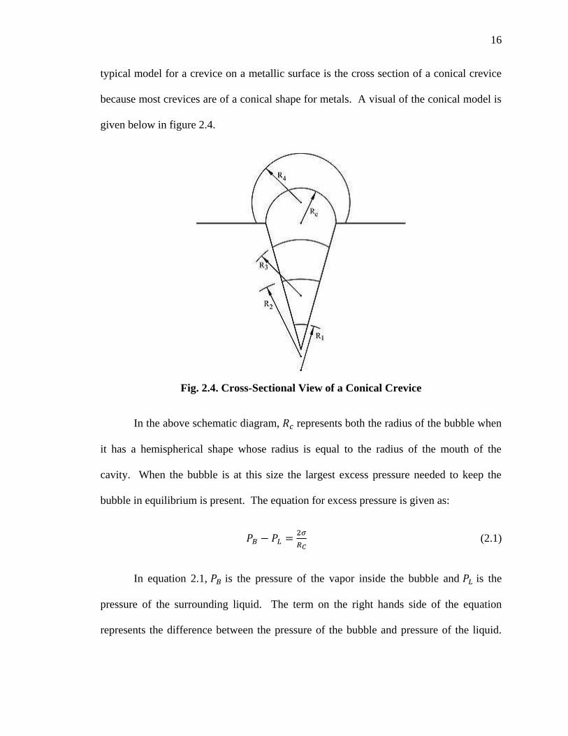
typical model for a crevice on a metallic surface is the cross section of a conical crevice
because most crevices are of a conical shape for metals. A visual of the conical model is
given below in figure 2.4.
Fig. 2.4. Cross-Sectional View of a Conical Crevice
In the above schematic diagram, represents both the radius of the bubble when
it has a hemispherical shape whose radius is equal to the radius of the mouth of the
cavity. When the bubble is at this size the largest excess pressure needed to keep the
bubble in equilibrium is present. The equation for excess pressure is given as:
(2.1)
In equation 2.1, is the pressure of the vapor inside the bubble and is the
pressure of the surrounding liquid. The term on the right hands side of the equation
represents the difference between the pressure of the bubble and pressure of the liquid.
17
The surface tension of the bubble holds the bubble together, keeping it in equilibrium
with the unbalanced pressure forces.
For a given fluid and conditions, the minimum and maximum crevice sizes that
will support the growth of a bubble can be calculated. A detailed derivation of the
equation is given in Ghiaasiaan (2008). The final equation for the crevice sizes, based on
the conditions and fluid properties, the equation for crevice sizes is as follows:
[ √
] (2.2)
(2.3)
(2.4)
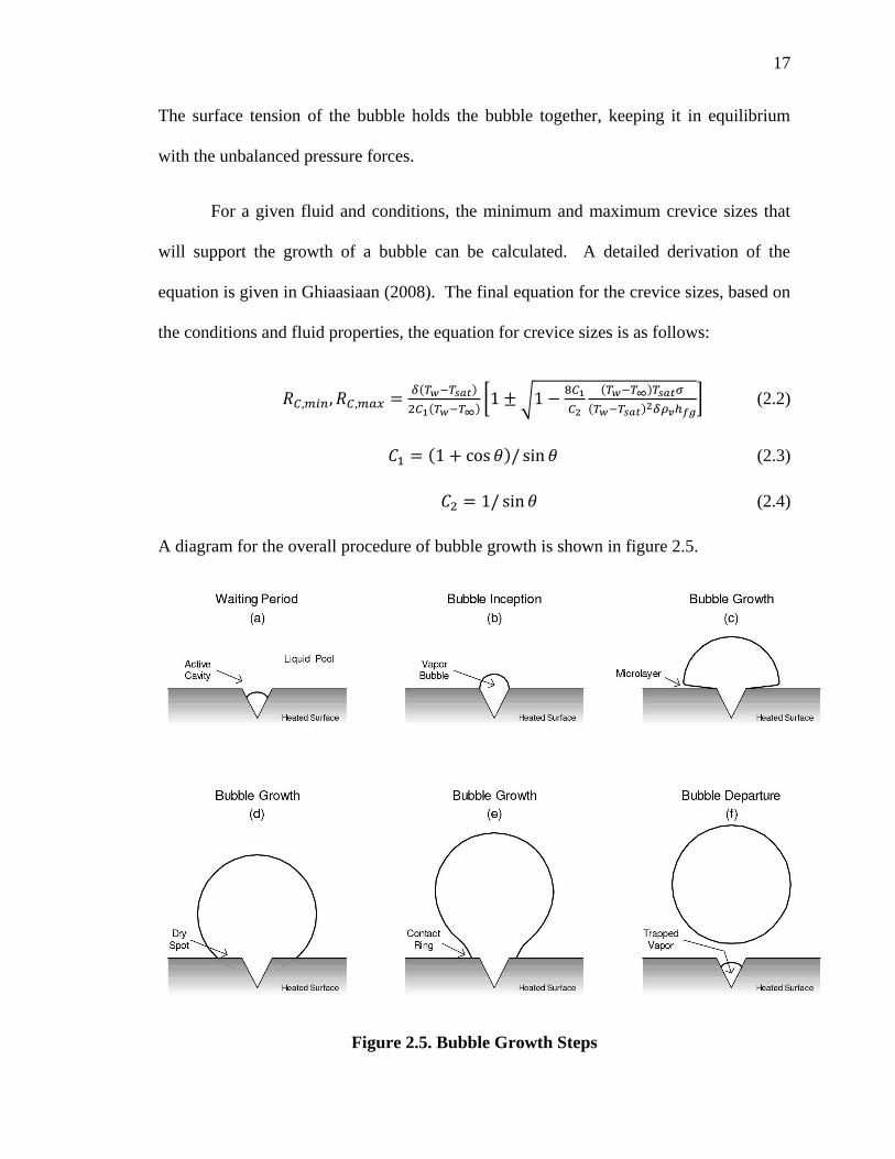
A diagram for the overall procedure of bubble growth is shown in figure 2.5.
Figure 2.5. Bubble Growth Steps

18
The first step in the process of bubble growth is the waiting period, step (a). It is
here that the bubble very small and grows inside the cavity by vaporization. When the
bubble grows to a radius equal to the radius of the cavity, it is said to be in the bubble
inception period, step (b). Steps (c), (d), and (e) are all known as the bubble growth
period. In these steps, liquid surrounding the bubble is being vaporized, which flows into
the bubble, making it larger and larger. Eventually, the bubble grows large enough that
the buoyancy forces pick the bubble up off of the surface and lift it away. This happens
in the final step, step (f), which is known as bubble departure. As soon as the bubble
departs, a new small bubble forms inside the crevice and the process of a boiling cycle
starts again. The speed at which this happens is based on the amount of heat flux.
Higher heat flux leads to a higher rate of bubble growth and departure.
As was discussed in the previous section regarding the experiments with nucleate
boiling on an inclined surface, the bubble growth and departure process is important only
at low to moderate heat fluxes. Especially in the downward facing cases (when the angle
of inclination is above ), the flow of the liquid over the surface comes into effect.
Bubbles still grow and depart at nucleation sites, but it is no longer the only mode of heat
transfer. At high heat fluxes near the CHF, bubble growth and departure is no longer
important at all. In the downward facing surface case, the bubbles become more apt to
coalescing with one another, forming a vapor blanket. Once the blanket has grown to a
large enough size, it slides off of the surface and a new blanket begins to form. This
process is far different from fluid mixing due to bubble growth and departure.

19
2.5 Nucleate Boiling Heat Flux Correlations
Theoretical models have not yet been developed for bubble dynamics that allow
us to make predictions for the nucleate boiling heat transfer coefficient. This is due to
uncertainties of the characteristics related to the boiling surfaces. Because of this,
empirical correlations are used to predict the nucleate boiling heat flux. This section will
briefly outline the most used correlations. Detailed derivations of these equations can be
found in Ghiaasiaan (2008).
Rohsenow (1952) developed a correlation that utilized the forced convection heat
transfer equation. The final correlation (which can be written in many different ways) is
given as:
[
√
]
(
)
(2.5)
In this correlation, whereas is a coefficient that is based on the
surface-fluid combination and is based on the fluid that is in use. This correlation
can be used to predict the nucleate boiling heat transfer, when the wall temperature is
known, to an accuracy of about 100%. The surface-fluid coefficient accounts for the
characteristics and wettability of the surface-fluid combination in use and could be a
good explanation of why the correlation is accurate and so widely used (Dhir, 1991).
Forster and Zuber (1954) developed a correlation for nucleate boiling heat flux
that, similar to Rohsenow, was based off of the Nusselt number, but in a more generic
form. The final equation for this correlation is as follows:

20
(
)
[
]
{
[
]
}
( )
(2.6)
(2.7)
The main difference between this correlation by Forster and Zuber (1955) and the
Rohsenow correlation is that this correlation does not account for surface effects. The
Rohsenow correlation contains a surface-fluid coefficient that accounts for those effects.
The Forster and Zuber correlation was used by Chen (1966) in the development of his
own correlation for forced convection nucleate boiling.
Stephan and Abdelsalam (1980) developed a series of Nusselt number
correlations to predict the nucleate boiling heat transfer. All of the correlations are rather
lengthy and are not shown here. A list of the equations can be found in Ghiaasiaan
(2008). There are separate correlations for hydrocarbons, water, selected refrigerants,
and cryogenic fluids. The correlations proposed by Stephan and Abdelsalam are reported
to have good accuracy.
Another correlation, developed by Cooper (1984) is much simpler than the
correlation proposed by Stephan and Abgelsalam (1980). Thome (2003) used this
correlation to make predictions for boiling newer refrigerants on copper tubes and found
that the correlation did not need any corrections to fit the results. They have used
Cooper’s correlation to account for the effects of nucleate boiling within flow boiling.
Cooper’s correlation is given as:
21
(
)
(2.8)
(2.9)
For this correlation, M is the molecular mass of the fluid and is the roughness
parameter.
Another nucleate boiling heat flux correlation was proposed by Gorenflo (1993).
The correlation is based solely on the fluid that is being boiled and has a recommended
range of parameters. It has been found to be very accurate with that range of parameters.
The general form of the correlation is as follows:
(2.10)
Most of the parameters in the above equation are specific to the fluid that is being
boiled. A table containing these parameters, as well as how to calculate and can be
found in Ghiaasiaan (2008).
The correlations given in this section are all heavily based on bubble dynamics on
an upward facing surface. As mentioned earlier, bubble dynamics change significantly
when the surface is inclined and is significantly different for a downward facing surface.
Because of this, none of the above equations are applicable to the current study. They
will not accurately predict the nucleate boiling heat flux on a downward facing surface.

22
2.6 Flow Boiling
Similar to the effects of natural convection, when a downward facing surface
heats up the ambient fluid, the fluid begins to flow along the surface. Pool boiling
involves an upward facing surface, where the bubbles, produced from evaporated liquid,
are free to flow upward with no obstruction. The bubble agitation is the only device that
is driving the heat transfer. In flow boiling, the mixing due to bubble growth and
departure along with the flowing fluid contribute to the heat transfer within the system.
Because of this, flow boiling is significantly more complicated than pool boiling. Similar
mixing effects occur for the case of nucleate boiling on a downward facing surface.
Figure 2.6 shows the different regions of flow boiling in a vertical channel, with
the fluid flowing upward, as well as the temperature profiles for the liquid and the wall.
Physical concepts from the bubbly flow and slug flow regions can be compared to
concepts for nucleate boiling on a downward facing surface.

23
Fig. 2.6. Flow Boiling Regimes and Temperature Profile in a Vertical Channel
The fluid enters the bottom of the channel as a single-phase liquid and exits the
top of the channel as a single-phase vapor. In the bubbly flow regime, when the single-
phase liquid has heated up enough to vaporize, small vapor bubbles begin to form on the
walls of the channel. Due to drag forces along the wall, the bubbles begin to peel off of
the wall and fill the channel. When the slug flow regime has been reached, the bubbles
begin to coalesce in the center of the channel, forming large vapor slugs. The vapor slugs

24
grow larger and larger as they move upward and, eventually, fill most of the channel. In
the annular flow regime, the slugs reach a growth point where they are so large that only
a thin liquid film remains along the walls. Helmholtz instabilities on the fluid-vapor
surface of the film cause small liquid ligaments to break off of the liquid film. The result
is a dispersed liquid phase in the center of the channel and a liquid film along the wall.
When the droplet flow regime has been reached, the liquid film along the walls has
vaporized and all that remains is a dispersed liquid that fills the channel. The liquid
droplets in the dispersed liquid eventually completely vaporize, resulting in a single-
phase vapor flow.
To the left and to the right of the vertical channel in figure 2.6 are the temperature
profiles and heat transfer regions of the fluid, respectively. In the single-phase
convective heat transfer and subcooled nucleate boiling heat transfer regions, the liquid is
heated from its initial temperature to its saturation temperature. During the single-phase
convective heat transfer, the wall temperature increases at the same rate as the fluid
temperature. The wall temperature remains (almost) constant from that point up to the
dryout point, coinciding with the droplet flow region. The fluid temperature remains
constant until after the dryout point and before the single-phase vapor heat transfer
region, where it begins to increase at a constant rate, as shown in the figure. At the
dryout point, the wall temperature begins to change at a non-constant rate, as shown in
the figure.
When vapor bubbles first start to appear, it is said that the onset of nucleate
boiling (ONB) point has been reached. At this point, heat transfer is controlled by both
nucleate boiling characteristics (from pool boiling) and flow characteristics. When the

25
slugs grow large enough to cause the liquid to form a film along the wall, this is known
as the departure from nucleate boiling (DNB) point. Nucleate boiling concepts no longer
apply after this point. In comparison to the flow boiling curve, the DNB point is
analogous to the CHF point. The study of nucleate boiling heat flux on a downward
facing surface shares similar characteristics as the flow boiling region between the ONB
and DNB points.
Flow boiling has also been studied in horizontal channels. While horizontal
channels present very similar characteristics to the vertical channel, they present new
concepts, some of which can be applied to nucleate boiling heat flux on a downward
facing surface. A schematic of flow boiling in a horizontal channel is shown below in
figure 2.7.
Fig. 2.7. Horizontal Flow Boiling Regimes
In general, the same flow regimes exist, as shown in figure 2.7. The regions of
interest for the current study are the bubbly flow and slug flow regions. The majority of
the vapor bubbles and vapor slugs are on the upper half of the channel. Just like in flow
boiling in a vertical channel, vapor bubbles form all the way around the channel
(including both top and bottom for the horizontal channel). Buoyancy forces the bubbles

26
formed on the lower surface to migrate towards the upper part of the channel.
Downstream of the ONB point, the bubbles begin to coalesce to form larger bubbles
(vapor slugs). Due to the presence of the upper wall, the vapor slugs flatten out to form a
pancake-like shape. The same phenomenon occurs for downward facing boiling. The
bubbles are forced upward due to buoyancy forces but the downward facing surface
restricts their upward motion. This is how the vapor blankets and elongated vapor slugs
are formed on the inclined surfaces.
2.7 Saturated Flow Boiling Characteristics in the Nucleate Boiling Regime
When a fluid is saturated, the quality of the fluid is somewhere between 0.0 and
1.0 and its temperature remains constant and equal to its saturation temperature. Quality
is the ratio of vapor mass to total mass of the system. By this definition, the quality of
the two-phase flow is 0.0 before the ONB point and is equal to 1.0 once all of the liquid
has vaporized. The contribution of forced convection becomes larger and larger as the
mass quality increases. In other words, nucleate boiling is significant only for low
qualities. Nucleate boiling takes place in the quality range of 0.0 up to a few percent,
where the CHF point is reached.
Many correlations have been developed that predict the heat transfer coefficient
for flow boiling. The correlations are, in general, very involved and contain many
constants. The correlations can be found in Ghiaasiaan (2008). Most of the correlations
are based off the summation rule that Chen (1966) proposed, which is:

27
(2.11)
where
(2.12)
The forced convection coefficient, , is generally calculated using a Nusselt
number correlation. The nucleate boiling heat transfer coefficient, , is calculated
using some combination of liquid, vapor, and two-phase flow quantities. For the case of
nucleate boiling on a downward facing surface, boiling induces flow along the
hemispherical surface. In the current study, nucleate boiling and flow boiling
characteristics have been lumped together into one equation. The Rohsenow (1952)
correlation for upward facing nucleate boiling captures both boiling and flow
characteristics. The flow characteristics are captured through the use of the Nusselt
number correlation, while the nucleate boiling characteristics are captured in the length
scales. In the present study, a method similar to what Rohsenow used is used in the
development of a correlation for nucleate boiling heat flux on a hemispherical, downward
facing surface. Both flow and boiling characteristics have been captured in order to
accurately predict the heat flux.
28
3. Upward Facing Boiling
3.1 Extension of Single-Phase to Two-Phase Heat Transfer
Single-phase fluid mechanics and heat transfer is very well understood by
engineers and researchers. In the discussion of multiple-phase heat transfer, however, the
same level of understanding has not been achieved. Many questions and problems arise
when figuring out how to treat the multi-phase mixture. An example of this arises when
calculating the friction factor for a two-phase flow of liquid and vapor. It is well known
and well documented as to how to make this calculation for single-phase flow. Rather
than developing a brand new way to make this calculation, researchers extended the
single-phase calculation into a two-phase calculation. Since drag is a product of viscous
effects, researchers found that the single-phase results can be extended to predict the two-
phase behavior by multiplying the single-phase friction factor by a coefficient that is a
function of viscosity. In particular, researchers used the bulk viscosity of the two-phase
mixture. McAdams et. al. (1942) developed a way to calculate this bulk viscosity in a
way that would coincide with experimental data.
Similar ideas have been employed in other two-phase flow cases. Boiling is one
such case where single-phase flow and heat transfer concepts are employed to make heat
transfer calculations. When boiling a pot of water on the stove, bubbles form on the
bottom of the pot and, at some point, release from the bottom and rise to the top. Water
exists and flows in multiple phases inside the pot – liquid and vapor. This classifies
boiling as a two-phase flow and heat transfer case. It is not easy to analytically evaluate
and predict boiling and the method in which to make calculations and predictions is not
29
trivial. The following sections explain how heat transfer calculations in upward facing
boiling are made through the extension from single-phase calculations to two-phase
calculations.
3.2 Nusselt Number Correlation
In the upward facing boiling case, the temperature of the heating surface is greater
than the saturation temperature of the fluid that it is above the surface. The difference
between the surface temperature and saturation temperature is known as the wall
superheat and, in equation form, is given as:
(3.1)
This temperature difference causes vapor bubbles to form on the surface of the
wall. As the bubbles grow, the buoyance force that pulls them away from the surface
also grows. When this force becomes larger than the surface tension force that holds the
bubble against the wall, the bubble releases. Liquid that was previously surrounding the
bubble fills in the void that the bubble has left. This process of vapor bubbles rising and
liquid taking its place causes agitation within the flow and increases the heat transfer
coefficient from the case of a heated wall with no boiling. Due to these concepts,
Rohsenow (1952) used the classic convective heat transfer correlation to predict the
boiling heat transfer, which is as follows:
(3.2)
The value for depends on whether the flow is in the laminar or turbulent
regime. This value ranges from 0.5 to 0.67, where 0.5 is for a laminar flow and 0.67 for a
30
turbulent flow. The above correlation is exactly the same correlation that is used for
single-phase heat transfer. The equation is derived using a scale analysis of the
continuity, Navier-Stokes, and energy equations of fluid mechanics. The Reynolds
number ( ) and Nusselt number ( ) and Prandtl number ( ) are defined as follows:
(3.3)
(3.4)
(3.5)
Substituting equations 3.3, 3.4, and 3.5 into equation 3.2 gives the following:
(
)
(
) (3.6)
3.3 Velocity, Length, and Temperature Scales
In order to complete the correlation, proper scales for the length ( ), velocity ( ),
and convection heat transfer coefficient ( ) had to be chosen. These scales were chosen
based on a physical analysis of the system.
The length scale chosen for the correlation is based off of the radius of the vapor
bubbles. From a pressure and surface tension force balance on a vapor bubble, the
following equation has been obtained:
(
) (3.7)
Where and are the minimum and maximum radii of a non-spherical bubble. For
the purposes of the analysis, the bubbles are assumed to be perfectly spherical. In other
words:
31
(3.8)
The pressure difference ( ) is the force generated from fluid head, where the height
used for this calculation is equal to twice the radius of the bubble:
(3.9)
Combining equations 3.8 and 3.9 with equation 3.7 and solving for gives the equation
for the length scale used in this analysis:
√
(3.10)
The next scale that was determined was the velocity scale. Rohsenow found this
by using a mass flow rate analysis. When a vapor bubble grows large enough, it
disconnects from the surface and surrounding liquid fills its place. Based on this, it was
determined that the mass flow rate of the vapor is equal to the mass flow rate of the
liquid. The equation for vapor mass flow rate is derived from the first law of
thermodynamics and is given as:
(3.11)
Where is the nucleate boiling heat flux and is the latent heat of vaporization.
The mass flow rate for the liquid is given as:
(3.12)
Setting the vapor and liquid mass flow rates equal to each other and solving for gives
the equation for the velocity scale:
(3.13)
32
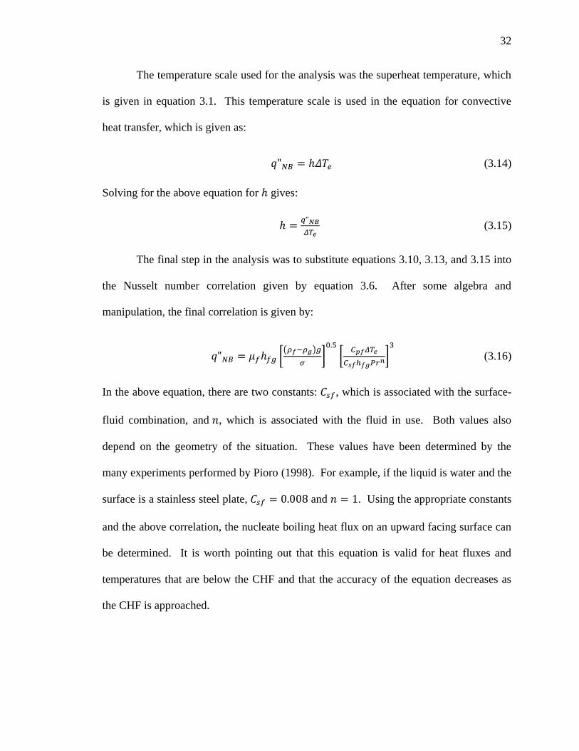
The temperature scale used for the analysis was the superheat temperature, which
is given in equation 3.1. This temperature scale is used in the equation for convective
heat transfer, which is given as:
(3.14)
Solving for the above equation for gives:
(3.15)
The final step in the analysis was to substitute equations 3.10, 3.13, and 3.15 into
the Nusselt number correlation given by equation 3.6. After some algebra and
manipulation, the final correlation is given by:
[( )
]
[
]
(3.16)
In the above equation, there are two constants: , which is associated with the surface-
fluid combination, and , which is associated with the fluid in use. Both values also
depend on the geometry of the situation. These values have been determined by the
many experiments performed by Pioro (1998). For example, if the liquid is water and the
surface is a stainless steel plate, and . Using the appropriate constants
and the above correlation, the nucleate boiling heat flux on an upward facing surface can
be determined. It is worth pointing out that this equation is valid for heat fluxes and
temperatures that are below the CHF and that the accuracy of the equation decreases as
the CHF is approached.

33
4. Downward Facing Boiling – Theoretical Work
4.1 Comparison to Upward Facing Boiling
The concept of downward facing boiling and its comparison to upward facing
boiling has been examined in the current study. The obvious major difference between
the two is the orientation and geometry of the surface. The upward facing boiling
correlation was derived based on an upward facing flat surface. The present study will
use similar concepts, but apply them to a downward facing surface. Fundamentally, both
cases have liquid in contact with a solid surface that is heated to the point of vaporization.
Bubbles grow on the surface of the solid then release from the surface when they have
grown to a large enough size.
Based on the similarities between the upward and downward facing boiling, the
same correlation has been used for the present study. The length and velocity scales,
however are different which will be discussed later. For convenience, the Nusselt
number correlation is written here again:
(4.1)
Once again, the Reynolds number determines the mixing effect of the flow and
the exponent provides an indication of whether the flow is in the laminar or turbulent
flow regime. The Prandtl number is a dimensionless measure of the size of the boundary
layer.
Similar to the upward facing boiling case, the Nusselt number correlation will be
transformed from a single-phase equation into a two-phase equation, based on a physical

34
analysis of the system. Single-phase heat transfer and fluid mechanics concepts will be
applied to the equation to make that transformation.
4.2 Development of Scales
There are two types of convective heat transfer: forced convection and natural
convection. In the forced convection case, the fluid is being forced over a surface and
heat transfer occurs at a rate dependent upon the boundary layer that forms along the
surface. In natural convection, the temperature difference between the fluid and the solid
surface causes a difference in density between the fluid near the surface and the fluid that
is away from the surface. This provides a driving force for the fluid motion. In the
present study, the temperature of the wall is warmer than the temperature of the fluid and,
therefore, the fluid that is near the wall flows upward under the influence of gravity. This
upward motion is an induced velocity in the fluid which causes convective heat transfer
to occur between the wall and the fluid.
The geometry under consideration is shown below in figure 4.1. The present
study involves buoyancy induced convection, which falls into the class of natural
convection. Suitable scales for the flow will be based off of a scale analysis of the
continuity, momentum, and energy equations of fluid mechanics, where the buoyancy
term is included in the momentum equation. For the forced convection case, the
buoyancy term does not appear in the momentum equation because it is small enough that
it can be neglected. The buoyancy term cannot be neglected for natural convection since
buoyancy is the driving force. The continuity, momentum, and energy equations used for
the present study are as follows:
35
Continuity:
(4.2)
Momentum:
(4.3)
Energy:
(4.4)
Fig. 4.1. Schematic of the Downward Facing Surface
Note that, in the buoyancy term in the momentum equation, the gravitational
acceleration is multiplied by . This is done in order to properly capture the effects
of gravity on the curved surface. At the bottom center of the surface, where ,
gravity does not have any effect on the flow. Gravity has the largest effect on the system
at the equator of the hemisphere, where is equal to unity.
After the appropriate governing equations and system geometry were established,
the scale analysis was performed. The first scale determined, was the temperature scale.
The temperature scale used in the present study is the same scale used in the Rohsenow

36
correlation. In the upward facing boiling case, the ambient fluid is heated to its saturation
temperature. The surface continues to heat up to some temperature that is hotter than the
fluid’s saturation temperature. This increased temperature causes vapor bubbles to form
on the heated surface. The same concept applies to the downward facing boiling case. A
suitable temperature scale is the wall superheat, which is defined again below for
convenience:
(4.5)
The next scale to be determined is the length scale. In single-phase flow and heat
transfer, the length scale is taken to be the local coordinate along the surface. For a flat
plate, the local coordinate is the distance from the leading edge to the location under
consideration. The same concept can be applied for the downward facing boiling case.
The bottom center of the hemisphere is the where the local coordinate is measured from
(analogous to the leading edge of a flat plate and the stagnation point in a crossflow
situation). The length scale for downward facing boiling is therefore chosen as:
(4.6)
The velocity scale is the last scale to be determined. Using the momentum
equation, given in equation 4.3, and focusing on the buoyancy term, a scale for the
velocity can be determined and is given as:
√ (4.7)
Note the similarities between the above velocity scale and the velocity scale used
for single-phase buoyancy driven heat transfer on a vertical flat plate. The single-phase
buoyancy driven heat transfer velocity scale is:

37
√ (4.8)
Both velocity scales are related to the local gravity, thermal expansion coefficient,
temperature difference, and local coordinate. The velocity scale for downward facing
boiling, given by equation 4.7, can be derived through a similar scale analysis. A
detailed description of the scale analysis is given in Appendix C. Through the
consideration of the flow geometry and temperature scale, the velocity scale was able to
be formulated to represent flow over a downward facing hemisphere in the case of
buoyancy driven heat transfer.
4.3 Development of the Nusselt Number Correlation
The final equation needed for the Nusselt number correlation is the relationship
between the nucleate boiling heat flux and the convective heat transfer coefficient. This
equation is given by:
(4.9)
The temperature (equation 4.5), length (equation 4.6), and velocity (equation 4.7)
scales along with equation 4.9 were substituted into the Nusselt number correlation. The
result is the correlation for nucleate boiling heat flux on a downward facing hemisphere,
which is given as:
( √
)
(4.10)
38
A detailed derivation of equation 4.10 is given in Appendix D. It is important to
note that the fluid properties in the correlation are the properties of the liquid which are to
be evaluated at the liquid saturation temperature and pressure.
The value for , which is the exponent of the Reynolds number, depends on
whether the flow is of the laminar or turbulent regime. This value should be chosen
based on the heat flux data that the equation is being fit to. The value of
corresponds to a laminar flow, whereas the value of corresponds to a turbulent
flow. This, once again, is a direct consequence of extending single-phase flow
characteristics into two-phase flow characteristics.
Equation 4.10 also shows the dependence of nucleate boiling heat flux on and
. These relationships are given as:
(4.11)
and
(4.12)
The correlation coefficient, , from equation 4.10 is dependent on the geometry
of the flow area. The velocity scale is dependent on the local coordinate, . The mass
flowrate, however, is a constant over the entire surface of the hemisphere. The equation
for mass flowrate is given as:
(4.13)
Due to mass continuity, the mass flowrate of the system must be a constant under
steady state conditions. Because the velocity of the flow is well below Mach 0.3 and the
39
temperature variation is small, the density is approximated as constant. The velocity and
flow area, however, are not constants and are dependent on the flow geometry. When
multiplied together, they must be equal to a constant in order to maintain a constant mass
flowrate. It follows that:
(4.14)
The area’s dependence on the local coordinate does not negate the velocity scale’s
dependence on the local coordinate, i.e.,
(4.15)
The velocity scale must be multiplied by a suitable coefficient in order to satisfy
the mass conservation. It follows that:
(4.16)
When the velocity scale is substituted into the Nusselt number correlation, it
carries the velocity scale coefficient, , with it. Because of this, the correlation
coefficient, , appearing in equation 4.10 becomes a function of a constant that is
independent of the local coordinate, multiplied by a coefficient that is dependent on the
local coordinate. The result is that the correlation coefficient , in equation 4.10, is a
function of the local coordinate. If the geometries of two different systems have separate
dependence on the local coordinate, the resulting correlation coefficients will also have
separate dependences on the local coordinate.

40
5. Downward Facing Boiling – Experimental Work
5.1 Overview of the Test Facility
To determine the correlation coefficient, , in equation 4.10, nucleate boiling data
for downward facing heating surfaces needed to be obtained experimentally. The test
facility used for these experiments was designed to imitate the reactor cavity in a nuclear
power plant. Figures 5.1 through 5.3 show the top, front, and side views of the water
tank that housed the test section with all of its dimensions. The main structure of the tank
is a cylinder large enough to house a simulated reactor pressure vessel (RPV) in the
center of the tank. A large cylindrical pipe was hung from the roof of the tank, where the
bottom of the pipe had a hemispherical shape and was positioned near the center of the
tank. A baffle structure was placed over the cylindrical pipe so as to mimic the
hydrodynamic effects of an ALWR.
Fig. 5.1. Top View of the Water Tank
41
Fig
5.3
. S
ide
Vie
w o
f th
e W
ate
r T
an
k
F
ig 5
.2. F
ron
t V
iew
of
the
Wate
r T
an
k

42
There are two large windows near the bottom of the tank and one small window
closer to the top of the tank. Images were captured through one of the large windows,
while proper lighting could be shined through the other large window. The small
window was placed near the top of the tank so that the water level could be monitored
easily while the tank was being filled up. It is important to note that the tank was made
from carbon steel. This material was chosen because of its strength, low material cost
and low manufacturing cost. Carbon steel, however, is susceptible to corrosion, so
proper care had to be taken in order to minimize the corrosion and keep clear
visualization of the flow.
A baffle structure was placed over top of the cylindrical pipe and hemisphere in
order to create a flow annulus. This baffle structure simulated the hydrodynamic effects
of the advanced light water reactor. Two sets of open slots were fabricated into the baffle
structure to allow for steam venting. The structure was made of plexi-glass so that it was
transparent and allowed for flow visualization and observation. Similar to the rest of the
tank, proper care had to be taken in order to keep it clean to not obstruct visualization.
One baffle structure was fabricated to simulate the AP600 baffle structure. Another
baffle structure was fabricated in order to simulate the KNGR baffle structure.
In order to simulate the decay heat from the reactor core melt, cartridge heaters
were welded to the inside of the aluminum hemispherical surface. The heat generated by
the cartridges was conducted to the water through the aluminum. Once the hemisphere
reached the desired temperature, the surrounding water started to boil. Six cartridge
heaters were welded to the middle portion of the hemisphere and eighteen more were
welded on the outer portion of the hemisphere, each having a power rating of 400W when

43
subjected to 120V. A maximum power level of 1.5MW/m2 was able to be achieved with
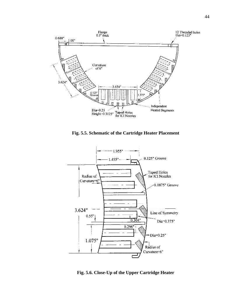
those cartridge heaters. Figures 5.4 through 5.6 show the configuration and dimensions
of the heater cartridges inside the hemisphere.
Fig. 5.4. Top View of the Cartridge Heater Placement
44
Fig. 5.5. Schematic of the Cartridge Heater Placement
Fig. 5.6. Close-Up of the Upper Cartridge Heater
45
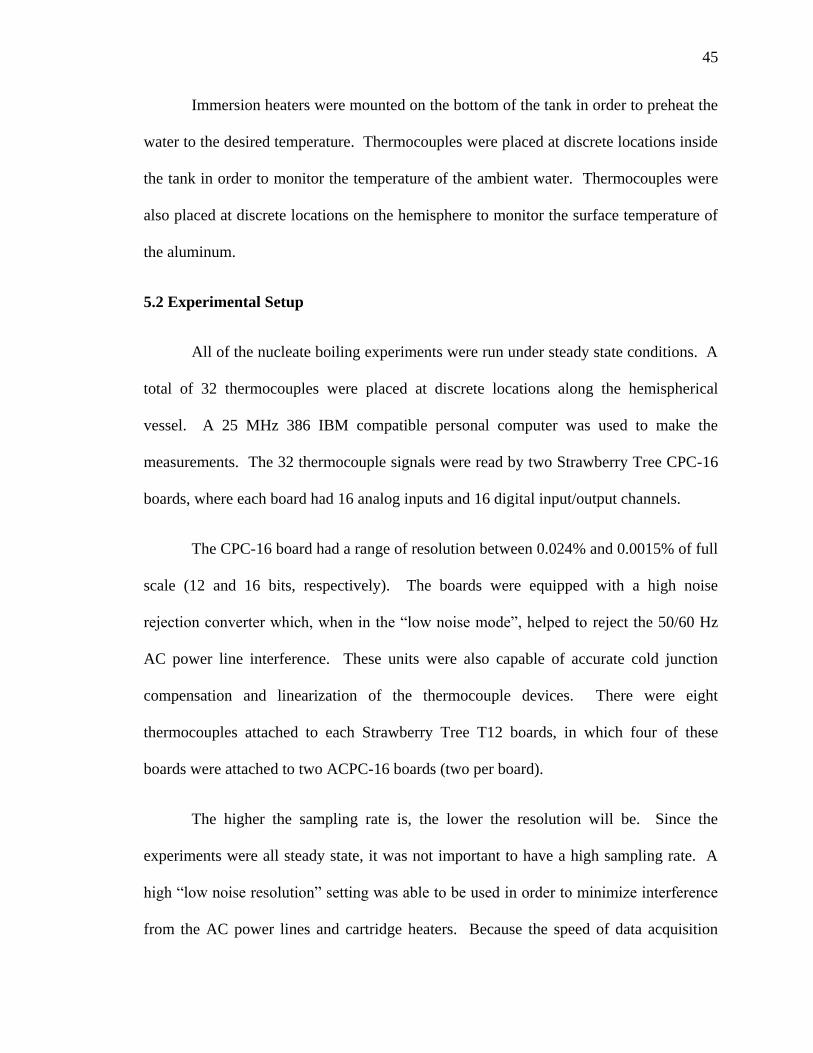
Immersion heaters were mounted on the bottom of the tank in order to preheat the
water to the desired temperature. Thermocouples were placed at discrete locations inside
the tank in order to monitor the temperature of the ambient water. Thermocouples were
also placed at discrete locations on the hemisphere to monitor the surface temperature of
the aluminum.
5.2 Experimental Setup
All of the nucleate boiling experiments were run under steady state conditions. A
total of 32 thermocouples were placed at discrete locations along the hemispherical
vessel. A 25 MHz 386 IBM compatible personal computer was used to make the
measurements. The 32 thermocouple signals were read by two Strawberry Tree CPC-16
boards, where each board had 16 analog inputs and 16 digital input/output channels.
The CPC-16 board had a range of resolution between 0.024% and 0.0015% of full
scale (12 and 16 bits, respectively). The boards were equipped with a high noise
rejection converter which, when in the “low noise mode”, helped to reject the 50/60 Hz
AC power line interference. These units were also capable of accurate cold junction
compensation and linearization of the thermocouple devices. There were eight
thermocouples attached to each Strawberry Tree T12 boards, in which four of these
boards were attached to two ACPC-16 boards (two per board).
The higher the sampling rate is, the lower the resolution will be. Since the
experiments were all steady state, it was not important to have a high sampling rate. A
high “low noise resolution” setting was able to be used in order to minimize interference
from the AC power lines and cartridge heaters. Because the speed of data acquisition
46
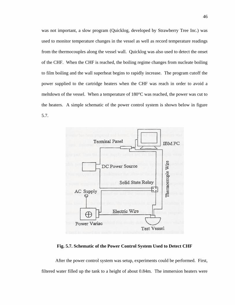
was not important, a slow program (Quicklog, developed by Strawberry Tree Inc.) was
used to monitor temperature changes in the vessel as well as record temperature readings
from the thermocouples along the vessel wall. Quicklog was also used to detect the onset
of the CHF. When the CHF is reached, the boiling regime changes from nucleate boiling
to film boiling and the wall superheat begins to rapidly increase. The program cutoff the
power supplied to the cartridge heaters when the CHF was reach in order to avoid a
meltdown of the vessel. When a temperature of 180°C was reached, the power was cut to
the heaters. A simple schematic of the power control system is shown below in figure
5.7.
Fig. 5.7. Schematic of the Power Control System Used to Detect CHF
After the power control system was setup, experiments could be performed. First,
filtered water filled up the tank to a height of about 0.84m. The immersion heaters were
47
turned on to heat the water to saturation temperature, and then left on for a few more
minutes to degas the water. The water was then allowed to cool back down to room
temperature before it was pumped through another filter to remove any precipitate
particles that the water attained during the heating process. The heaters were turned back
on to heat the water back up to saturation temperature.
Once the water was heated to the desired temperature, the baffle structure was
lowered into the water, followed by the hemisphere and cylindrical pipe. Next, the power
supply cables were connected to the adjustable power suppliers and the thermocouple
wires were attached to the data acquisition system. The power system was then turned on
in order to start heating the hemisphere, while temperatures at the various locations were
monitored. Once it was decided that steady state had been reached, Quicklog began
recording the temperatures from each thermocouple and stored them for analysis. Once
the CHF was reached, the program ended the experiments.
5.3 Experimental Results
The raw data gathered by Quicklog is presented in Appendix C and Appendix D.
Appendix C displays the downward facing boiling data taken with the AP600 baffle
around the hemisphere, while Appendix D displays the data taken with the KNGR baffle
around the hemisphere. The data has also been plotted in figures 5.8 and 5.9, where
figure 5.8 shows the AP600 data and figure 5.9 shows the KNGR data. For the KNGR
data, the nucleate boiling heat flux increases with increasing wall superheat to a certain
point and levels off (except at ). Where the data levels off is the CHF point.
Note that the heat flux value does not change, but the wall superheat continues to

48
increase. This is the point that Quicklog shuts off the power supplied to the heaters to
end the experiment. For the AP600 data, the data shows signs of leveling off near a heat
flux of 1MW/m2 at high angles. This is an indication that the data is approaching the
CHF.
When the data levels off and the wall superheat rapidly increases with no change
in the heat flux, the boiling mechanism has transitioned from nucleate boiling to film
boiling. At these heat flux levels, a thin vapor layer forms between the liquid and the
heating surface. Because no liquid is physically touching the heating surface, the surface
temperature increases rapidly. Vapor transfers heat at a much slower rate than liquid,
causing the sudden temperature increases.
For both baffle structures, the nucleate boiling heat flux increases with increasing
angle at constant temperature. This occurs due to the increasing influence of buoyancy
forces on the flow. The buoyancy forces increase due to the angle of inclination of the
heating surface. Gravity acts in only the vertical direction, so, as the angle increases, the
heating surface becomes more and more vertically oriented, causing the increase in
buoyancy forces.
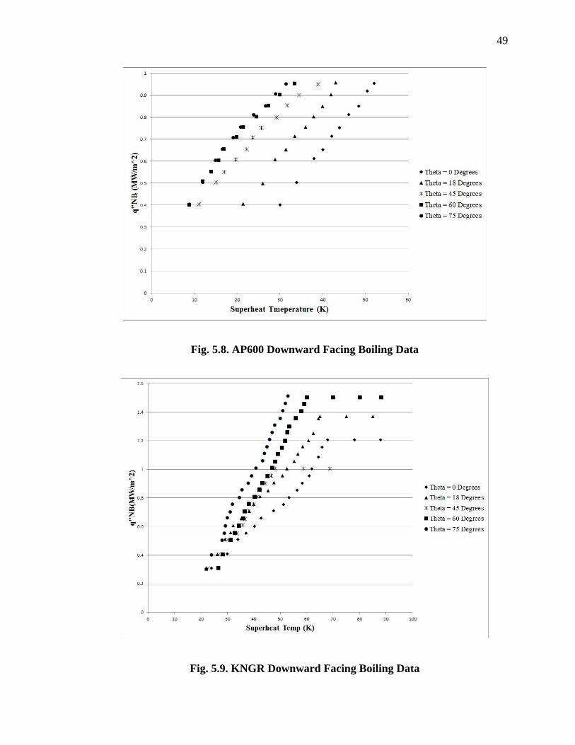
49
Fig. 5.8. AP600 Downward Facing Boiling Data
Fig. 5.9. KNGR Downward Facing Boiling Data
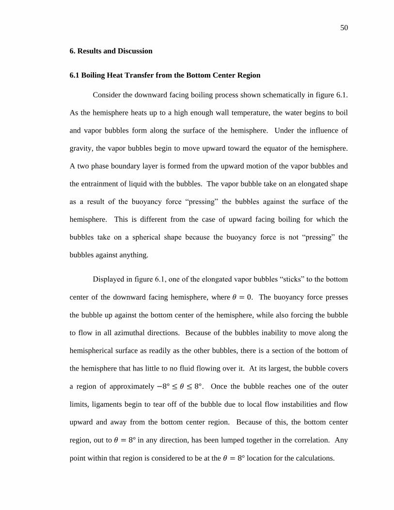
50
6. Results and Discussion
6.1 Boiling Heat Transfer from the Bottom Center Region
Consider the downward facing boiling process shown schematically in figure 6.1.
As the hemisphere heats up to a high enough wall temperature, the water begins to boil
and vapor bubbles form along the surface of the hemisphere. Under the influence of
gravity, the vapor bubbles begin to move upward toward the equator of the hemisphere.
A two phase boundary layer is formed from the upward motion of the vapor bubbles and
the entrainment of liquid with the bubbles. The vapor bubble take on an elongated shape
as a result of the buoyancy force “pressing” the bubbles against the surface of the
hemisphere. This is different from the case of upward facing boiling for which the
bubbles take on a spherical shape because the buoyancy force is not “pressing” the
bubbles against anything.
Displayed in figure 6.1, one of the elongated vapor bubbles “sticks” to the bottom
center of the downward facing hemisphere, where . The buoyancy force presses
the bubble up against the bottom center of the hemisphere, while also forcing the bubble
to flow in all azimuthal directions. Because of the bubbles inability to move along the
hemispherical surface as readily as the other bubbles, there is a section of the bottom of
the hemisphere that has little to no fluid flowing over it. At its largest, the bubble covers
a region of approximately . Once the bubble reaches one of the outer
limits, ligaments begin to tear off of the bubble due to local flow instabilities and flow
upward and away from the bottom center region. Because of this, the bottom center
region, out to in any direction, has been lumped together in the correlation. Any
point within that region is considered to be at the location for the calculations.

51
Fig
. 6.1
. S
chem
ati
c of
Tw
o-P
hase
Bou
nd
ary
Layer
52
6.2 Values Chosen for and Physical Implications
Past experimental results indicate that, in the Nusselt number correlation, the
exponent on the Reynolds number is an indication of the flow regime of the fluid under
consideration. If the flow is laminar, the exponent will be 0.5, whereas the exponent will
be 0.67 if the flow is turbulent. In this study, different values of were chosen for the
AP600 and KNGR correlations in order to have the correlation follow the trend of the
data. For the AP600 correlation, the value for was found to be 0.5, indicating laminar
flow. For two-phase flow, a large amount of mixing is expected. Because of this, it was
unexpected that the data indicated that the flow was laminar. For the KNGR data, a value
of 0.67 was chosen for , indicating that the flow was turbulent.
6.3 Nucleate Boiling Heat Flux Dependence on and with Value for
The dependence on and , with respect to , of the nucleate boiling heat flux
was calculated in chapter 4. For convenience, the correlation and the result of the
calculation is shown again below.
( √
)
(6.1)
(6.2)
(6.3)
With the value of for the AP600 correlation, the dependence on and
for the nucleate boiling heat flux is:
53
(6.4)
(6.5)
With the value of for the KNGR correlation, the dependence on and
for the nucleate boiling heat flux is:
(6.6)
(6.7)
It is interesting to note that, in terms of for the KNGR correlation, the nucleate
boiling heat flux loses its dependence on by itself, and depends on only .
6.4 Correlation Coefficient’s Dependence on
At any particular angle, the correlation coefficient is a constant. At varying
angles, however, the correlation coefficient is not a constant. Figures 6.2 and 6.3 show
the correlation coefficient as a function of the angle on the hemisphere (in essence, the
local position along the hemisphere). The correlation coefficient for the AP600
correlation has a linear relationship with angle and is as follows:
(6.8)
The correlation coefficient for the KNGR correlation, on the other hand, has a cubic
relationship with angle and is as follows:
(6.9)
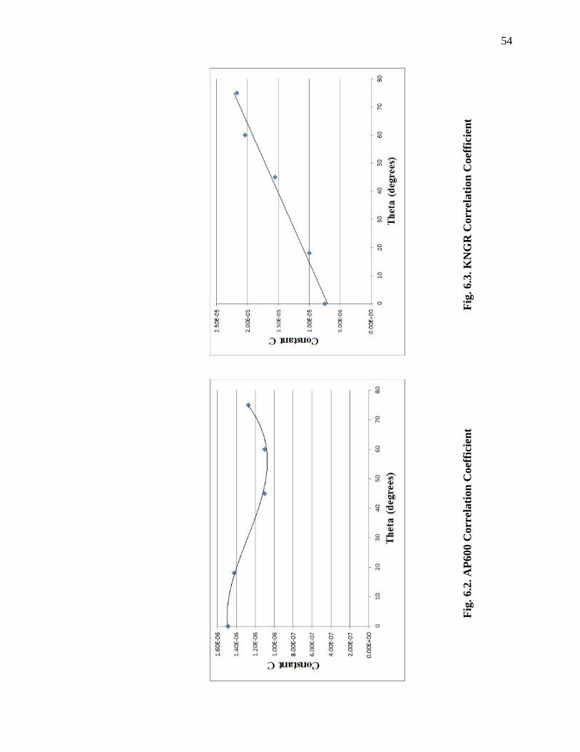
54
Fig
. 6.2
. A
P600 C
orr
elati
on
Coef
fici
ent
F
ig. 6.3
. K
NG
R C
orr
elati
on
Coef
fici
ent

55
The difference in the relationship between the correlation coefficient and angle for the
AP600 and KNGR correlations demonstrates the difference in flow area geometries
between the two cases. The flow area geometry for the AP600 case is a more simple
geometry compared to the KNGR flow geometry. In the KNGR case, the minimum gap
between the baffle and the hemispherical surface occurs between the angles of 50˚ and
70˚. There is a “dip” on the plot for the KNGR correlation coefficient between those two
angles. This is evidence that the gap is small enough to affect the nucleate boiling heat
flux. In the AP600 case, the minimum gap is not small enough to have significant
interference with the flow. This is why the relationships between the correlation
coefficient and the angle do not follow the same trends.
6.5 Comparison of the Proposed Correlation with the Measured Data
Figures 6.4 through 6.8 show the comparison between the experimental nucleate
boiling heat flux data and the correlation for the AP600 case. The correlation matches
the experimental data very well for all wall superheats and heat fluxes for the angles of 0
and 18 degrees. At angles of 45 degrees and larger, the correlation matches the data well
up to a heat flux of about 0.8MW/m2. The plots show that, as the data approaches the
CHF, the slope of the data quickly decreases and no longer follows the trend of the
correlation. The slope decreases due to the boiling mechanism transitioning from
nucleate boiling to film boiling. The slope bends until it is flat and the large temperature
jumps occur when the CHF point is reached. This puts a limit on the range of validity of
the correlation for the nucleate boiling correlation for the AP600 case. The correlation,
therefore, is valid up to a nucleate boiling heat flux value of about 0.8MW/m2.

56
Fig
. 6.4
. A
P600 H
eat
Flu
x D
ata
at 𝜽
𝟎

57
Fig
. 6.5
. A
P600 H
eat
Flu
x D
ata
at 𝜽
𝟏𝟖
F
ig. 6.6
. A
P600 H
eat
Flu
x D
ata
at 𝜽
𝟒𝟓

58
Fig
. 6.7
. A
P600 H
eat
Flu
x D
ata
at 𝜽
𝟔𝟎
Fig
. 6.8
. A
P600 H
eat
Flu
x D
ata
at 𝜽
𝟕𝟓

59
Figures 6.9 through 6.13 show the comparison between the experimental nucleate
boiling heat flux data and the correlation for the KNGR case. The effects of the extreme
flow geometry are evident in the plots. The CHF value starts high, about 1.2MW/m2,
decreases to about 1MW/m2, then rises back up to above 1.5MW/m
2. The nucleate
boiling heat flux approaches the CHF with a different slope in each case. The difference
in slope is reflected in the correlation coefficient plot. The nucleate boiling heat flux
tends to decrease around the 50˚ mark, and then increases again around the 70˚ mark.
Note that the correlation for KNGR agrees very well with the measured data at all
angular positions.
Fig. 6.9. KNGR Heat Flux Data at
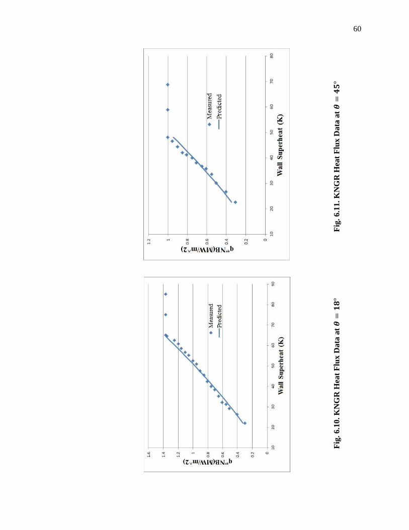
60
Fig
. 6.1
0. K
NG
R H
eat
Flu
x D
ata
at 𝜽
𝟏𝟖
Fig
. 6.1
1.
KN
GR
Hea
t F
lux D
ata
at 𝜽
𝟒𝟓
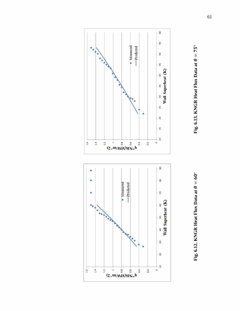
61
Fig
. 6.1
2. K
NG
R H
eat
Flu
x D
ata
at 𝜽
𝟔𝟎
Fig
. 6.1
3. K
NG
R H
eat
Flu
x D
ata
at 𝜽
𝟕𝟓
62
7. Conclusions and Recommendations
7.1 Overall Behavior of Buoyancy Driven Convection
Nucleate boiling on a downward facing surface possesses the behaviors of single-
phase buoyancy driven flow and heat transfer, as well as two-phase phenomena and
phenomena unique to downward facing boiling. Based on the results of this study, the
following conclusions can be made:
The wall superheat causes a difference in density between the liquid and the
hemispherical heating surface, leading to buoyancy driven flow and heat transfer.
Vapor bubbles, which are formed along the external surface of the hemisphere,
depart from the surface once they have reached their mature sizes.
A large bubble (vapor blanket) forms at the bottom center of the hemisphere in
the region of which is treated as one lumped vapor mass in the
analysis.
The single-phase Nusselt number correlation, length scale, and velocity scale can
be utilized in the two-phase analysis.
The correlation coefficient, , was determined empirically in the analysis and
reflects the geometry of the flow. In particular, the empirical correlation indicates
whether or not the minimum gap is significantly small and the approximate
location of the minimum gap if it is significantly small.
The value of in the correlation is chosen such that the correlation fits the data
and serves as an indication of laminar ( or turbulent ( ) flow.
63
7.2 Extension of Single-Phase Flow and Heat Transfer to Two-Phase Flow and Heat
Transfer
In the analysis of nucleate boiling on a downward facing surface, single-phase
concepts and phenomena were used to extend a single-phase analysis into a two-phase
analysis. Buoyancy driven flow and heat transfer has been studied extensively in basic
fluid mechanics and heat transfer. In the case of downward facing boiling, the two-phase
phenomenon arises from the liquid being vaporized near the external surface of the
heated hemisphere, resulting in a two-phase boundary layer flow along the surface. The
same buoyancy driven flow and heat transfer concepts for the single-phase case apply for
the two-phase case. As a fluid’s temperature increases, the density of the fluid decreases.
Under the influence of the Earth’s gravitational field, the less dense fluid will flow
upward and the two-phase boundary layer is a consequence of the fluid motion. Utilizing
single-phase concepts and equations, suitable length and velocity scales were developed
for the two-phase, downward facing boiling case. The corresponding analysis and
equations are provided in chapter 4 as well as Appendices A and B.
7.3 Range of Validity of the Correlation
Similar to the Rohsenow correlation, the correlation for nucleate boiling on a
downward facing surface is not valid over the entire nucleate boiling region for all cases.
The correlation very accurately predicts the nucleate boiling heat flux up to a heat flux of
approximately 0.8MW/m2 for the AP600 case. For the KNGR data, the correlation is
valid over the entire nucleate boiling heat flux region. It is important to remain within
the bounds of validity of the correlation in order to make accurate heat flux predictions,
64
as well as avoid making costly errors in heat flux predictions. Errors could result in a
design that would not provide sufficient cooling of the RPV by downward facing boiling
which would lead to a meltdown of the reactor vessel.
7.4 Recommendations for Future Work
The following work items are recommended for future effort:
Develop a method of calculating the correlation coefficient, , through a flow
geometry and mass flowrate analysis.
Run experiments using different materials for the hemisphere and different
ambient fluids to determine the correlation’s dependence on these parameters.
Determine the correlation’s dependence on the Prandtl number, , and the
exponent of the Prandtl number, .
Develop a correlation (or modify the current correlation) accounting for the effect
of subcooled boiling, where the ambient fluid is at a temperature that is less than
the saturation temperature.
Validate the correlation with more data from cases with different baffle structures
(differing flow geometries).
65
REFERENCES
1. Beduz, C., Scurlock, R. G. and Sousa, A. J., 1988, “Angular dependence of boiling
heat transfer”, Advances in Cryogenic Eng., R. W. Fast, ed., Plenum Press, New
York, Vol. 33, pp. 363-370.
2. Chen, J. C., 1966, “Correlation for boiling heat transfer to saturated fluids in
convective flow”, Ind. Eng. Chem. Res., Vol. 5, pp. 322-329.
3. Chen, Li-Ting, 1978, “Heat transfer to pool boiling Freon from inclined heating
plate”, Lett Heat Mass Transfer, Vol. 5, pp. 111-120.
4. Cooper, M. G., 1984, “Saturated nucleate pool boiling – A simple correlation”, First
UK National Heat Transfer Conf., Inst. Chem. Eng. Symp. Ser. 86, Vol. 2, pp. 785-
793.
5. Dhir, V. K., 1991, “Nucleate and transition boiling heat transfer under pool and
external flow conditions”, Int. J. Heat Fluid Flow, Vol. 12, pp. 290-314.
6. Forster, H. K., and Zuber, N., 1954, “Growth of a vapor bubble in a superheated
liquid”, J. Appl. Phys., Vol. 25, pp. 474-478.
7. Forster, H. K., and Zuber, N., 1955, “Dynamics of vapor bubbles and boiling heat
transfer”, Chem. Eng. Prog., Vol. 1, No. 4, pp. 531-535.
8. Ghiaasiaan, S. M., 2008, “Two-phase flow, boiling, and condensation in
conventional and miniature systems”, Cambridge University Press, pp. 302-354.
9. Gorenflo, D., 1993, “Pool boiling”, In VDI-Heat Atlas (English Version), Schlünder,
E. U., Ed., pp. Ha 1-13, VDI-Verlag, Düsseldorf, Germany.
66
10. Haddad, K.H., Liu, Y. C., and Cheung, F. B., 1995, “Spatial variation of critical heat
flux on a downward facing hemispherical surface”, Proc. 1995 National Heat
Transfer Conference, Vol. 14, GTD-vol. 316, pp. 23-32.
11. Ishigai, S., Inoue, K., Kiwaki, Z. and Inai, T., 1961, “Boiling heat transfer from a flat
surface facing downward”, Int. Heat Transfer Conf., Aug. 29-Sep. 1, Paper No. 26.
12. Jung, D. S., Venart, J. E. S. and Soussa, A. C. M., 1987, “Effects of enhanced
surfaces and surface orientation on nucleate and film boiling heat transfer in R-11”,
Int. J. Heat Mass Transfer, Vol. 30, No. 2, pp. 2627-2639.
13. Liu, Y. C., 1999, “Buoyancy-Driven Co-Current Two-Phase Flow in a
Hemispherical Annular Channel With Natural Convection Boiling on the Downward
Facing Side”, PhD Dissertation, Department of Mechanical Engineering, The
Pennsylvania State University.
14. Marcus, B. D. and Dropkin, D., 1963, “The effect of surface configurations on
nucleate boiling heat transfer”, Int. J. Heat Mass Transfer, Vol. 6, pp. 863-867.
15. McAdams, W. H., Woods, W. K. and Heroman, L.C., Jr., 1942, “Vaporization inside
horizontal tubes – II – Benzene – oil mixtures”, Trans. ASME, Vol. 64, pp. 193-200.
16. Nishikawa, K., Fujita, Y., Uchida, S. and Ohta, H., 1984, “Effect of surface
configuration on nucleate boiling heat transfer”, Int. J. Heat Mass Transfer, Vol. 27,
No. 9, pp. 1559- 1571.
17. Nishio, S. and Chandratilleke G. R., 1989, “Steady-state pool boiling heat transfer to
saturated liquid helium at atmospheric pressure”, JSME Int. J., Series I, Vol. 23, No.
4, pp. 639-645.
67
18. Pioro, I. L., 1998, “Experimental evaluation of constants for the Rohsenow pool
boiling correlation”, Int. J. Heat Mass Transfer, Vol. 42, pp. 2003-2013.
19. Rohsenow, W. M., 1952, “A method of correlation heat transfer data for surface
boiling of liquids”, Trans. ASME, Vol. 74, pp. 969-975.
20. Stephan, K., and Abdelsalam, M., 1980, “Heat-transfer correlations for natural
convection boiling”, Int. J. Heat Mass Transfer, Vol. 23, pp. 73-87.
21. Theofanous, T., Liu, C., Addition, S., 1996. In-Vessel Coolability and Retention of a
Core Melt. DOE/ID-10460.
22. Vishnev, I. P., Filatov, I. A., Vinokur, Ya. G., Gorokhov, V. V. and Svalov, G. G.,
1976, “Study of heat transfer in boiling of Helium on surfaces with various
orientations”, Heat Transfer, Soviet Research, Vol. 8, No. 4, pp. 104-108.

68
Appendix A – Scale Analysis of Buoyancy Driven Flow Along a Downward Facing
Surface
The first equation used in the scale analysis is the continuity (mass conservation)
equation.
Continuity:
(A.1)
Each variable in the equation can be scaled as follows:
(A.2)
(A.3)
(A.4)
(A.5)
The scale for the velocity in the y direction ( ) is unknown. In terms of the local
length and velocity scales, the derivatives in the continuity equation can be scaled as
follows:
(A.6)
(A.7)
In order to conserve mass,
and
must be on the same order as each other, i.e.,
(A.8)
69
Using the scales above, the following relationship is expected:
(A.9)
A suitable scale for can now be determined as
(A.10)
At this point, a suitable scale for the velocity in the direction ( ) has yet to be
determined. A scale analysis of the momentum equation provides a suitable scale for .
Momentum:
(A.11)
Using the same scales as above, each term of the equation can be scaled as
follows:
(A.12)
(A.12)
(A.13)
(A.14)
The advection terms on the left hand side of the momentum equation must be
balanced by the diffusion and buoyancy terms on the right hand side of the equation. A
balance between the advection and buoyancy terms gives:
(A.15)

70
Solving this equation for ( ) yields the velocity scale used for the downward
facing boiling analysis:
√ (A.16)
The Nusselt number correlation can be derived from a scale analysis of the energy
equation, which is shown below in equation A.17.
Energy:
(A.17)
The temperature scale is the wall superheat. The scales for the advection terms
are as follows:
(A.18)
(A.19)
Note that the y coordinate now scales as , which is the local thickness of the
thermal boundary layer. Substituting equation A.10 into equation A.19 yields:
(A.20)
At saturation temperature, the Prandtl number for water is on the order of one
( ). This allows the following assumption to be made:
(A.21)

71
Using this assumption, substituting equation A.21 into equation A.20, and
simplifying, it becomes apparent that the two advection terms are on the same order as
each other.
(A.22)
The diffusion term on the right hand side of the energy equation can be
approximated as:
(A.23)
The advection and diffusion terms must balance each other in the energy
equation. It follows that:
(A.24)
Solving equation A.24 for yields the following expression:
(
)
(A.25)
The conductive heat flux scale is given by:
(A.26)
The convective heat flux is equal to the convection heat transfer coefficient
multiplied by the temperature difference (i.e. the wall superheat) as shown below:
(A.27)
72
Substituting equation A.27 into equation A.26 and solving for gives:
(A.28)
Substituting equation A.28 into equation A.25 gives the following relationship:
(
)
(A.29)
In order to make equation A.29 nondimensional, both sides of the equation must
be divided by a suitable length scale. Dividing by the local length scale, , makes the
most sense. This yields:
(
)
(A.30)
The term on the left hand side of equation A.30 is the inverse Nusselt number,
while the term on the right hand side of the equation somewhat resembles a Reynolds
number. Multiplying the right hand side by (
)
completes the Reynolds number.
Inversing and simplifying the equation gives:
(
)
(
)
(A.31)
Since the two sides of this equation are of the same order, the right hand side of
the equation can be multiplied by a constant in order to make both sides equal. The three
terms in equation A.31 are the Nusselt number, Reynolds number, and Prandtl number.
The final equation is as follows:
(A.32)

73
Note that the exponents on the Reynolds number and Prandtl number have been
changed to and , respectively. This was done since the correlation was derived for
laminar flow conditions. If turbulent flow conditions exist, the exponents will need to be
determined experimentally.
74
Appendix B – Detailed Derivation of Downward Facing Boiling Correlation
The Nusselt number correlation derived in Appendix A is shown again below for
convenience:
(B.1)
The definition of what the Nusselt number, Reynold’s number, and Prandtl
number will now be filled in to the above correlation.
(
)
(
)
(B.2)
The equation for the nucleate boiling convective heat transfer coefficient is shown
below:
(B.3)
The length and mass scales, that were developed in Appendix A, are written again
below for convenience:
(B.4)
√ (B.5)
Substituting equations B.3, B.4, and B.5 into equation B.2 yields the following
equation:
⁄
(
(√ )
)
(
)
(B.6)
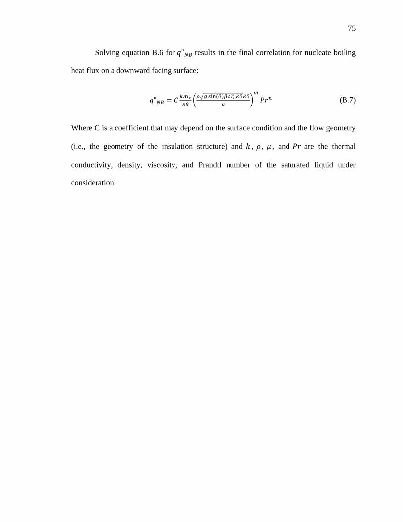
75
Solving equation B.6 for results in the final correlation for nucleate boiling
heat flux on a downward facing surface:
( √
)
(B.7)
Where C is a coefficient that may depend on the surface condition and the flow geometry
(i.e., the geometry of the insulation structure) and , , , and are the thermal
conductivity, density, viscosity, and Prandtl number of the saturated liquid under
consideration.

76
Appendix C. Raw Data for AP600
Table C.1: Steady State Saturated Nucleate Boiling Data at the Bottom Center
Tw - Tsat (°C) Measured q"NB (MW/m2) Predicted q"NB (MW/m
2)
30.1012 0.4008 0.4611
34.0225 0.5016 0.5373
38.0558 0.6102 0.6181
40.1011 0.6511 0.6599
42.2106 0.7120 0.7035
44.0254 0.7505 0.7416
46.1089 0.8115 0.7857
48.5157 0.8501 0.8373
50.5158 0.9177 0.8807
52.1144 0.9524 0.9157
53.5088 1.0120 0.9464

77
Table C.2: Steady State Saturated Nucleate Boiling Data at
Tw - Tsat (°C) Measured q"NB (MW/m2) Predicted q"NB (MW/m
2)
21.5004 0.4053 0.4023
26.0782 0.4985 0.5120
28.9623 0.6075 0.5838
31.5014 0.6531 0.6484
33.4953 0.7134 0.7001
36.0775 0.7552 0.7682
37.9573 0.8024 0.8186
40.0112 0.8503 0.8743
42.0021 0.9025 0.9290
43.0568 0.9563 0.9583
44.0412 1.0320 0.9858
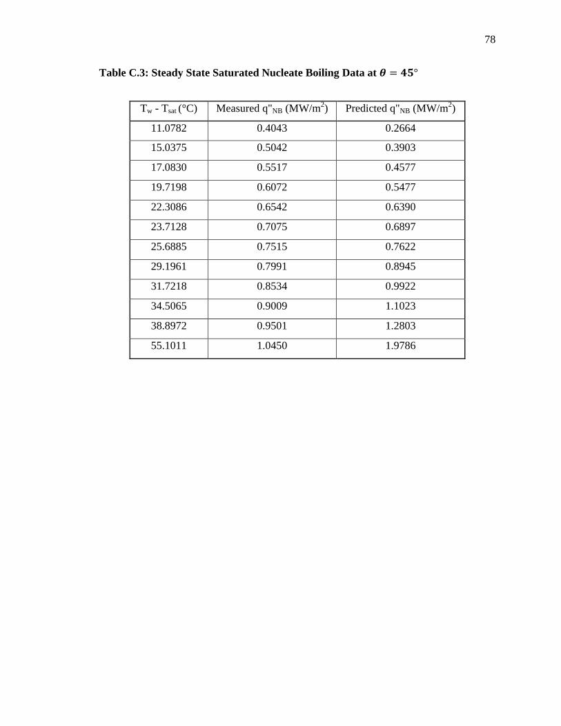
78
Table C.3: Steady State Saturated Nucleate Boiling Data at
Tw - Tsat (°C) Measured q"NB (MW/m2) Predicted q"NB (MW/m
2)
11.0782 0.4043 0.2664
15.0375 0.5042 0.3903
17.0830 0.5517 0.4577
19.7198 0.6072 0.5477
22.3086 0.6542 0.6390
23.7128 0.7075 0.6897
25.6885 0.7515 0.7622
29.1961 0.7991 0.8945
31.7218 0.8534 0.9922
34.5065 0.9009 1.1023
38.8972 0.9501 1.2803
55.1011 1.0450 1.9786

79
Table C.4: Steady State Saturated Nucleate Boiling Data at
Tw - Tsat (°C) Measured q"NB (MW/m2) Predicted q"NB (MW/m
2)
8.8845 0.4007 0.2602
12.1133 0.5068 0.3834
14.0204 0.5518 0.4602
15.7976 0.6019 0.5342
17.0668 0.6536 0.5885
20.0189 0.7084 0.7183
21.5249 0.7524 0.7865
24.6077 0.8013 0.9298
27.4036 0.8506 1.0636
30.1076 0.9010 1.1964
33.5086 0.9516 1.3677
37.0790 1.0070 1.5522

80
Table C.5: Steady State Saturated Nucleate Boiling Data at
Tw - Tsat (°C) Measured q"NB (MW/m2) Predicted q"NB (MW/m
2)
8.9001 0.4026 0.2701
12.1025 0.5013 0.3966
14.0457 0.5493 0.4777
15.0865 0.6020 0.5224
16.7010 0.6525 0.5932
19.1877 0.7059 0.7056
20.8955 0.7534 0.7849
24.0125 0.8094 0.9339
26.7901 0.8502 1.0708
29.1130 0.9032 1.1881
31.5136 0.9501 1.3118
33.5126 1.0450 1.4167
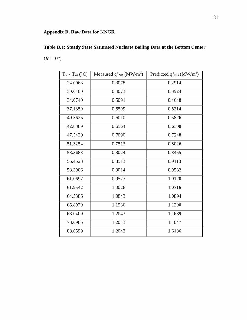
81
Appendix D. Raw Data for KNGR
Table D.1: Steady State Saturated Nucleate Boiling Data at the Bottom Center
Tw - Tsat (°C) Measured q"NB (MW/m2) Predicted q"NB (MW/m
2)
24.0063 0.3078 0.2914
30.0100 0.4073 0.3924
34.0740 0.5091 0.4648
37.1359 0.5509 0.5214
40.3625 0.6010 0.5826
42.8389 0.6564 0.6308
47.5430 0.7090 0.7248
51.3254 0.7513 0.8026
53.3683 0.8024 0.8455
56.4528 0.8513 0.9113
58.3906 0.9014 0.9532
61.0697 0.9527 1.0120
61.9542 1.0026 1.0316
64.5386 1.0843 1.0894
65.8970 1.1536 1.1200
68.0400 1.2043 1.1689
78.0985 1.2043 1.4047
88.0599 1.2043 1.6486

82
Table D.2: Steady State Saturated Nucleate Boiling Data at
Tw - Tsat (°C) Measured q"NB (MW/m2) Predicted q"NB (MW/m
2)
22.0679 0.3019 0.3273
26.2928 0.4039 0.4134
29.1418 0.5093 0.4742
31.3394 0.5563 0.5225
32.2232 0.6057 0.5422
35.3118 0.6545 0.6126
38.4089 0.7059 0.6852
40.0648 0.7549 0.7249
42.4050 0.8082 0.7819
45.5015 0.8508 0.8590
47.6457 0.9066 0.9133
50.8744 0.9551 0.9968
52.5874 1.0033 1.0418
55.2894 1.0562 1.1138
56.6729 1.1082 1.1511
58.4889 1.1582 1.2005
60.7288 1.2005 1.2622
62.6098 1.2511 1.3146
64.5446 1.3530 1.3690
65.0227 1.3701 1.3826
75.0512 1.3701 1.6740
85.0666 1.3701 1.9783
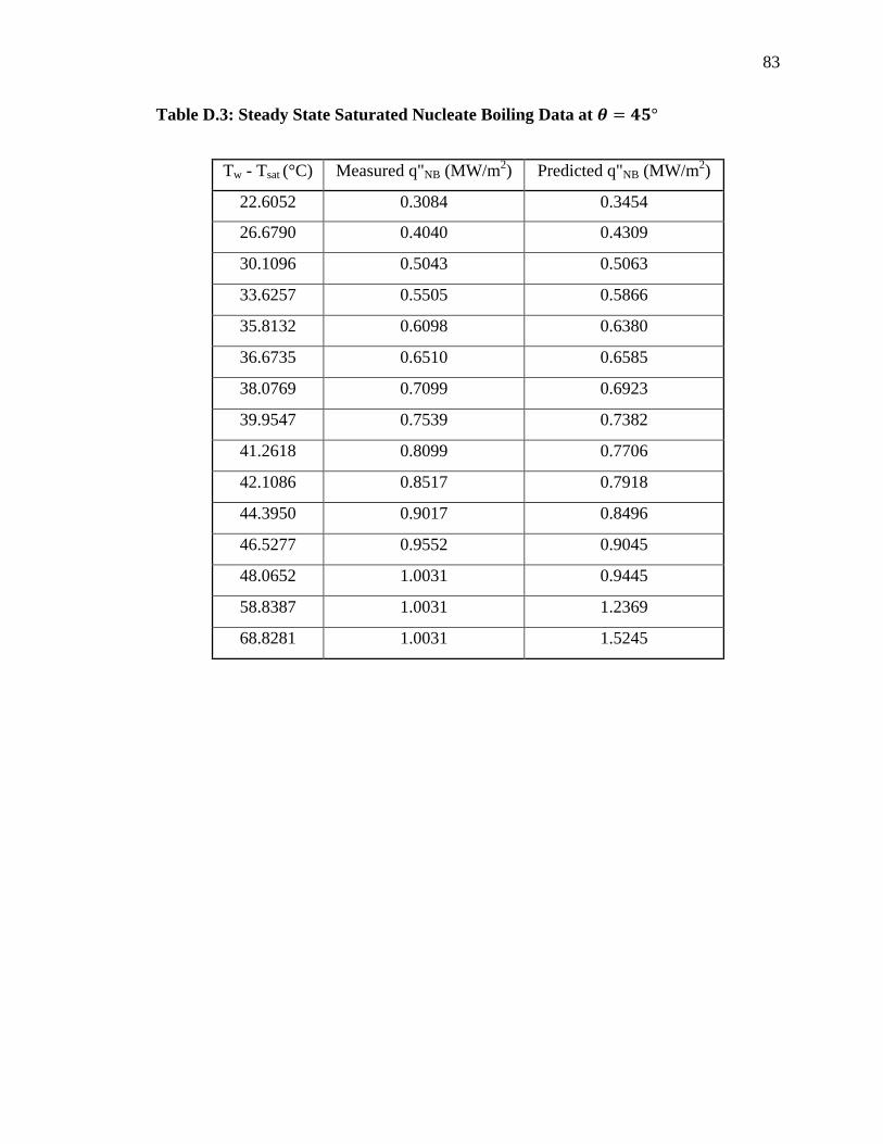
83
Table D.3: Steady State Saturated Nucleate Boiling Data at
Tw - Tsat (°C) Measured q"NB (MW/m2) Predicted q"NB (MW/m
2)
22.6052 0.3084 0.3454
26.6790 0.4040 0.4309
30.1096 0.5043 0.5063
33.6257 0.5505 0.5866
35.8132 0.6098 0.6380
36.6735 0.6510 0.6585
38.0769 0.7099 0.6923
39.9547 0.7539 0.7382
41.2618 0.8099 0.7706
42.1086 0.8517 0.7918
44.3950 0.9017 0.8496
46.5277 0.9552 0.9045
48.0652 1.0031 0.9445
58.8387 1.0031 1.2369
68.8281 1.0031 1.5245

84
Table D.4: Steady State Saturated Nucleate Boiling Data at
Tw - Tsat (°C) Measured q"NB (MW/m2) Predicted q"NB (MW/m
2)
26.5475 0.3098 0.4591
28.1675 0.4062 0.4969
31.2878 0.5055 0.5716
32.8276 0.5550 0.6094
34.3827 0.6047 0.6482
36.0774 0.6567 0.6911
36.5925 0.7069 0.7043
38.0877 0.7585 0.7429
40.2661 0.8058 0.8001
42.0630 0.8588 0.8481
43.2953 0.9048 0.8814
45.2100 0.9534 0.9337
47.0559 1.0097 0.9849
48.0803 1.0543 1.0136
49.0611 1.1068 1.0412
50.6078 1.1511 1.0852
51.8892 1.2002 1.1220
52.7551 1.2584 1.1471
53.4349 1.3007 1.1668
55.8913 1.3556 1.2389
58.0143 1.4059 1.3020
59.0687 1.4573 1.3337
60.0868 1.5025 1.3644
70.0032 1.5025 1.6726
80.1203 1.5025 2.0024
88.1355 1.5025 2.2739
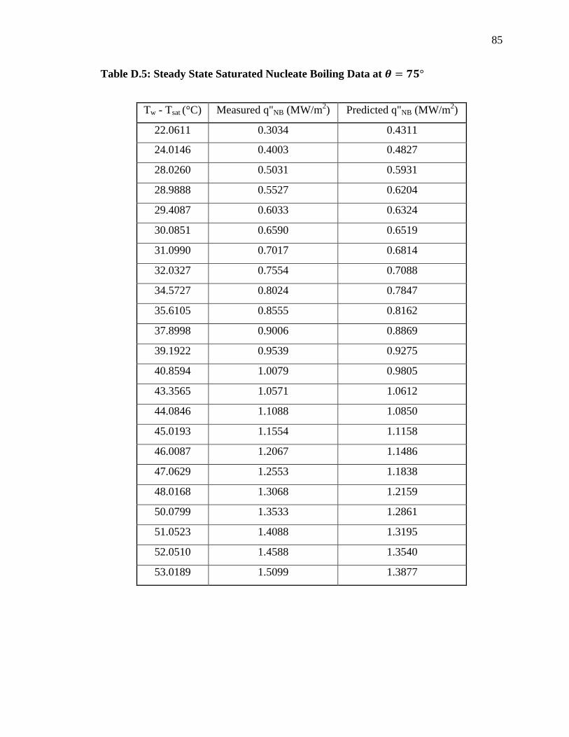
85
Table D.5: Steady State Saturated Nucleate Boiling Data at
Tw - Tsat (°C) Measured q"NB (MW/m2) Predicted q"NB (MW/m
2)
22.0611 0.3034 0.4311
24.0146 0.4003 0.4827
28.0260 0.5031 0.5931
28.9888 0.5527 0.6204
29.4087 0.6033 0.6324
30.0851 0.6590 0.6519
31.0990 0.7017 0.6814
32.0327 0.7554 0.7088
34.5727 0.8024 0.7847
35.6105 0.8555 0.8162
37.8998 0.9006 0.8869
39.1922 0.9539 0.9275
40.8594 1.0079 0.9805
43.3565 1.0571 1.0612
44.0846 1.1088 1.0850
45.0193 1.1554 1.1158
46.0087 1.2067 1.1486
47.0629 1.2553 1.1838
48.0168 1.3068 1.2159
50.0799 1.3533 1.2861
51.0523 1.4088 1.3195
52.0510 1.4588 1.3540
53.0189 1.5099 1.3877
Recommended