Download pdf - Development of a 3-component Load Cell for Structural Impact Testing

Development of a 3-component load cell for structural impact testing

A. G. HANSSEN1,2,*, T. AUESTAD1, M. LANGSETH1 and T. TRYLAND3

1Structural Impact Laboratory (SIMLab), Department of Structural Engineering, Norwegian University of Science and

Technology (NTNU), N-7491, Trondheim, Norway; 2SINTEF Materials Technology, Rich Birkelandsvei 2B, N-7465,

Trondheim, Norway; 3Hydro Automotive Structures, N-2831, Raufoss, Norway

*Author for correspondence (E-mail: [email protected])

Abstract. This paper describes the development of a 3-component load cell for structural impact testing. The test

specimen is mounted directly on the load cell, which measures the axial force as well as two orthogonal bending

moments. Basically, the load cell is a stocky cylinder with thick end flanges machined in one piece of high-strength steel.

The load measurement system is based upon four strain gauges glued to the central shaft. The signal from each strain

gauge is sampled separately. Afterwards, this data is used to compute the axial force and the bending moments. The load

cell was originally developed for testing of automotive components.

Key words: load cell, impact, energy absorption, crash testing, ls-dyna

1. Introduction

The objective of this study was to develop a cost-effective load cell, which could be applied for

high-speed offset testing of bumper systems. A description of the test set-up using the load cell is

given by Hanssen et al. (2003). The final load cell design is shown in Figure 1. The load cell is

machined from one piece of high-strength steel with a minimum yield stress of r0=600 MPa

(proportionality limit). Four strain gauges are evenly distributed on the perimeter in the middle-

plane of the central shaft. The shaft is a stocky, hollow cylinder of circular cross-section and

with a wall thickness and outer diameter of 7 mm and 100 mm, respectively. Both ends of the

central shaft are connected to thick flanges (80 mm). Such a thickness is necessary in order to

realise a linear strain distribution (Euler-Bernoulli) over the cross section in the central shaft,

which forms the basis for the calibration formulas given below, Section 3. The required flange

thickness was determined by use of numerical simulations, see Section 2.2. The load cell has 5

spherical indents machined into the front flange, which are for calibration purposes. Here,

compressive load is applied to the load cell through a steel ball successively located in all five

holes, see illustration in Figure 3. This yields sufficient information to fully calibrate the load

cell statically, Section 3. The rear flange has a hollow, circular cross section and incorporates six

threaded M16 holes for fastening to an external surface. The frontal flange has a square cross

section and is fitted with four 11 mm holes, one in each corner, to accommodate the test

specimens. The requirements for the load-cell were as follows: (1) Capacity of 200 kN at a load

eccentricity of 100 mm, (2) Natural frequency of system should be above 400 Hz and (3)

Accuracy in average force level within ±5%.

International Journal of Mechanics and Materials in Design (2005) 2: 15–22 � Springer 2006

DOI 10.1007/s10999-005-0513-z

2. Load cell design

2.1. CAPACITY FOR ECCENTRIC LOADING

The capacity N of a hollow, circular cylinder as function of the load eccentricity e, Figure 3,

(assuming a linear strain distribution over the cross section and neglecting transversal shear) is

given by

N

N0¼ 1

1þ2 ed

12� h

dþ hd

� �2� �ð1Þ

where d is the outer diameter and h is the wall thickness. N0 is the capacity for pure-axial loading

given by N0 =r0 A where r0 is the yield stress and A is the cross sectional area.

195

115

160 x 160

80

0

ø11

R22

.2

80

19

5

80

35

16

0

50

55

Ø130

ø160

ø100

ø86

40

4

M16

65

Ø11

65

160

50

50

50

55

Rear view

Front view

Side view

Section view

Strain-gauge location

Front

Rear

Figure 1. Load-cell design.

16 A.G. Hanssen et al.

2.2. LINEAR STRAIN DISTRIBUTION

The influence of the flange thickness on the strain distribution over the cross section of the load

cell can be seen from Figure 2(a). These results are based on numerical simulations by use of the

non-linear, finite element code LS-DYNA (Hallquist, 1998). The loading was applied through a

sphere, located 50 mm from the symmetry axis of the load cell. In Figure 2(a), the stress

distribution is given for three different values of the flange thickness, B=20, 40 and 100 mm.

The axial stress on the outer-wall in the middle-plane of the central shaft is denoted by rz. The

corresponding average value of the axial stress for all x/d ratios is denoted by �rz. The stress

distribution rz=�rz is given as a function of x/d, where x is the coordinate as defined in Fig-

ure 2(b). The data points of Figure 2 are based on the axial stress at the integration point of the

volume elements located on the perimeter of the load cell. As can be seen, the stress distribution

is highly non-linear for flange thicknesses of 20 and 40 mm. For B=100 mm, the stress dis-

tribution is practically linear. The final load cell was made with a flange thickness of 80 mm.

Figure 2(b) shows the stress distribution for this case. Assume that the signal from the four

strain gauges (rz0, rz90, rz180, rz270) relates to the axial stress of four brick elements located on

the perimeter of the load cell, see illustration of Figure 2(b). Let the corresponding average

value be denoted by �rSz ¼ rz0 þ rz90 þ rz180 þ rz270ð Þ=4. In order for the strain gauges to give a

good representation of the true axial force then �rSz � �rz. For Figure 2b one finds that

�rSz =�rz ¼ 1:0057. On can also imagine that the set of four strain gauges is rotated an angle h

relative to the axis of loading, Figure 2(b). The average strain-gauge signal is now

�rSz ¼ rz0þh þ rz90þh þ rz180þh þ rz270þhð Þ=4. By varying h from 0 to 90 degrees it was found that

the error margins are 0:9949 < �rSz =�rz < 1:0057. Hence the error appears to be well within ±1%

for a load eccentricity of 50 mm. Figure 2(b) also shows the strain distribution for central

loading. For this case the distribution is practically linear. The load cell�s instrumentation is not

able to capture transversal shear forces or any axial twisting moments. On the other hand, the

occurrence of such reactions should not cause the instrumentation to record any significant axial

σ σ

-1 -0.8 -0.6 -0.4 -0.2 0 0.2 0.4 0.6 0.8 1

-1

0

1

2

3

4

5

B = 20 mm40 mm

100 mm

B

z

z

/x d

-1 -0.8 -0.6 -0.4 -0.2 0 0.2 0.4 0.6 0.8 1

-1

0

1

2

3

4

z

z

σ σ

/x d

e = 0

e = 50 mm

90zσ

0zσ

180zσ

270zσ

0z σ +

90z σ +

180z σ +

270z σ +

y

xN

Straingauge

Cross section of load cell (central part)

0zσ

90zσ

180zσ

270zσ e

(b)(a)

θθ

θ

θ

θ

Figure 2. (a) Cross-section strain distribution for various flange thicknesses, eccentric loading (e=50 mm). (b) Strain

distribution of final load cell design (flange thickness B=80 mm.)

Development of a 3-component load cell 17

forces or bending moments. In the same manner as described above, the load cell was subjected

to a pure shear force at the top flange. The maximum axial force recorded for strain-gauge

locations 0� < h < 90� were 0.69, 9.68 and 36.6 kN for shear force levels of 100, 200 and

300 kN, respectively. For shear force levels higher than 250 kN the strain distribution in the

central shaft of the load cell is no longer linear. Finally, the load cell was subjected to a pure

twisting moment. For twisting moments of 10, 20, 30 and 40 kNm the recorded maximum axial

force measure was 0.2, 0.6, 1.2 and 1.8 kN, respectively. Again, this is insignificant.

2.3. DYNAMIC BEHAVIOUR

The dynamic behaviour of the load cell was studied numerically by use of LS-DYNA. First, an

eigenvalue analysis was carried out using the same finite element model as described above. The

frequency response in terms of the five lowest eigenfrequencies was: 1.53, 1.53, 1.63, 3.025 and

3.025 kHz. The two lowest eigenmodes correspond to bending of the central shaft around

orthogonal axes. A similar behaviour is also observed for modes four and five. The third

eigenmode is axial twisting. The range of applicability (loading rate) of the load cell will be

governed by the cell�s lowest eigenfrequency fe. Assume that the loading takes place at a velocity

v0 and that the impacted structure shows an oscillating force vs. time response with a charac-

teristic period Ts. This is typical for an axially loaded extrusion. For such a structure the

characteristic period Ts is given by the loading velocity v0 and the half-plastic lobe length of

deformation L, i.e. Ts=2L/v0. For a hollow, square extrusion L � bðh=bÞ1=3 (Jones, 1989) givingTs � 2bðh=bÞ1=3=v0. Here b and h are the width and thickness of the extrusion respectively.

Assume that loading is to take place at frequency ratios ðfeTsÞ�1 < 0:2 to keep the amount of

dynamic magnification below 5% (SDOF-system, no damping (Clough and Penzien, 1975)),

then v0 < 0:4febðh=bÞ1=3. Using fe=1.53 kHz, b=80 mm, h=2 mm yields v0<14.3 m/s, which

conforms well with the set-up used for 40% bumper testing (15 m/s), Hanssen et al. (2003).

The initial loading at impact may take place quicker, i.e. in this case the first peak load

recorded by the load cell may be influenced by the cell�s own response.

3. Calibration formulas

Assume a linear-strain distribution in the shank of the load cell for a general eccentric loading

condition, Figure 3. Let the original voltage signal from the four strain gauges be

v0 ¼ v01; v02; v

03; v

04

� �Twhere the subscripts specifies the strain gauge. The output from the

amplifier is then v ¼ av0 ¼ a1v01; a2v

02; a3v

03; a4v

04

� �T¼ v1; v2; v3; v4f gT. The axial strain in the

location of the strain gauges is proportional to voltage, hence e ¼ e1; e2; e3; e4f gT¼kv ¼ k1v1; k2v2; k3v3; k4v4f gT. The four voltage signals of v ¼ v1; v2; v3; v4f gT are sampled sep-

arately and post-processed in order to determine the reaction forces on the load cell.

3.1. CALIBRATION STEP 1: AXIAL FORCE

Assume a state of pure-axial loading (e=0). The axial force N is related to the axial strain e by

N ¼ �KNe where �KN is the axial stiffness. For this loading condition there are four measures for

the axial strain, e ¼ ei ¼ kivi; i ¼ 1::4. In this way there are also four measures for the axial

force, N ¼ �KNei ¼ �KNkivi ¼ Kivi; i ¼ 1::4. The state of pure-axial loading will provide data for

calibration of the constants Ki , i=1..4, see Section 4, Figure 4(a–d). An eccentrically applied


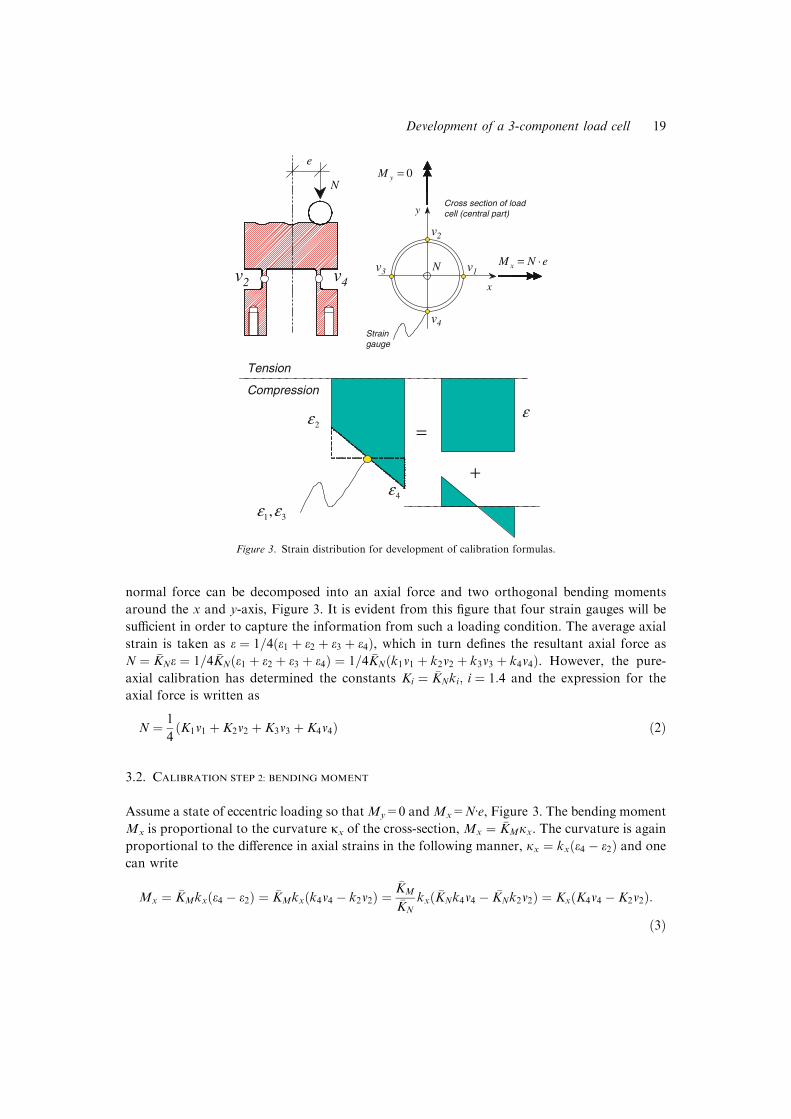
normal force can be decomposed into an axial force and two orthogonal bending moments

around the x and y-axis, Figure 3. It is evident from this figure that four strain gauges will be

sufficient in order to capture the information from such a loading condition. The average axial

strain is taken as e ¼ 1=4 e1 þ e2 þ e3 þ e4ð Þ, which in turn defines the resultant axial force as

N ¼ �KNe ¼ 1=4 �KN e1 þ e2 þ e3 þ e4ð Þ ¼ 1=4 �KN k1v1 þ k2v2 þ k3v3 þ k4v4ð Þ. However, the pure-

axial calibration has determined the constants Ki ¼ �KNki; i ¼ 1:4 and the expression for the

axial force is written as

N ¼ 1

4K1v1 þ K2v2 þ K3v3 þ K4v4ð Þ ð2Þ

3.2. CALIBRATION STEP 2: BENDING MOMENT

Assume a state of eccentric loading so thatMy=0 andMx=NÆe, Figure 3. The bending moment

Mx is proportional to the curvature jx of the cross-section, Mx ¼ �KMjx. The curvature is again

proportional to the difference in axial strains in the following manner, jx ¼ kx e4 � e2ð Þ and one

can write

Mx ¼ �KMkx e4 � e2ð Þ ¼ �KMkx k4v4 � k2v2ð Þ ¼�KM

�KNkx �KNk4v4 � �KNk2v2ð Þ ¼ Kx K4v4 � K2v2ð Þ:

ð3Þ

Tension

Compression

4ε

2ε =

+

1 3,ε ε

ε

N

e

v2 v4

y

x

v1v3

v2

v4Straingauge

Cross section of load cell (central part)

xM N e=

0yM =

N.

Figure 3. Strain distribution for development of calibration formulas.


0 200 400 600 800

0

100

200

300

400

500N (kN)

0 200 400 600 800

0

100

200

300

400

500

Axialloading

N (kN)

0 200 400 600 800

0

100

200

300

400

500

0 200 400 600 800

0

100

200

300

400

500

Axialloading

N (kN)

Gauge 2

(mV)

K2 = 0.730 kN/mV

Gauge 3

(mV)

K3 = 0.836 kN/mV

(b)

(c)

Axialloading

Gauge 4

(mV)

K4 = 0.761 kN/mV

-15 -10 -5 0 5 10 15

-15

-10

-5

0

5

10

15

0xK

0xM

= 0.0078

-15 -10 -5 0 5 10 15

-15

-10

-5

0

5

10

15

= 0.0018 0yK

0y

-1000 0 1000

-15

-10

-5

0

5

10

15

0 50 100 150 200 250

0

50

100

150

200

250

Eccentric loading

0 50 100 150 200 250

0

50

100

150

200

250

Applied force (kN)

Model (kN)

Check of axial force. Pos. 2

Applied force (kN)

Model (kN)


Eccentric loading

0 50 100 150 200 250

0

50

100

150

200

250

Applied force (kN)

Model (kN)


My (kNm)

(kN)

Nm)

Nm)

Ky = 0.0100 m

( )1 1 3 3K v K v

(a)

Eccentric loading

Axialloading

(i) (e)

(k( )4 4 2 2xK K v K v

(kNm)

(k( )1 1 3 3yK K v K v

(kNm)

K1 = 0.821 kN/mV

N (kN)

(mV)

Gauge 1

0 50 100 150 200 250

0

50

100

150

200

250

Eccentric loading


Model (kN)

Applied force (kN)

-10

-

-

-

-

00 0 1000

-15

-10

-5

0

5

10

15

Kx = 0.0109 m

(kN) ( )4 4 2 2K v K v

Mx (kNm)

(f ) (j)

(g ) (k)

(d) (h) (l)

Figure 4. Results from calibration procedure.


Hence, Mx ¼ Kx K4v4 � K2v2ð Þ where the constants K2 and K4 have already been determined by

the pure-axial loading condition in Section 3.1. Eccentric loading around the x-axis will provide

data for determination of Kx. The same consideration can be used for eccentric loading around

the y-axis and one arrives at My ¼ Ky K1v1 � K3v3ð Þ. The results for the current load cell are

given in Section 4, Figure 4(i–j).

If the strain gauges are not correctly positioned, a moment around the x-axis will induce

strains in the strain gauges used for calculation of moment around the y-axis and vice versa.

However, this coupling effect can also be taken into consideration by the calibration formulas.

Assume that the load cell has been subjected to an axial force and moment only around the x-

axis. The computed bending moment around the x-axis is then Mx ¼ Kx K4v4 � K2v2ð Þ. Thecalculated moment around the y-axis is M0

y ¼ Ky K1v1 � K3v3ð Þ, where the superindex is used to

indicate that this is a residual moment. This error can be related to the computed bending

moment Mx in the following manner M0y ¼ K0

yMx ¼ K0y � Kx K4v4 � K2v2ð Þ, which easily deter-

mines Ky0. The residual moment My

0 has to be subtracted from the original expression

My ¼ Ky K1v1 � K3v3ð Þ. In this way, the complete formulas for the bending moment around the

x- and y-axis read

Mx ¼ Kx K4v4 � K2v2ð Þ � K0x � Ky K1v1 � K3v3ð Þ ð4Þ

and

My ¼ Ky K1v1 � K3v3ð Þ � K0y � Kx K4v4 � K2v2ð Þ: ð5Þ

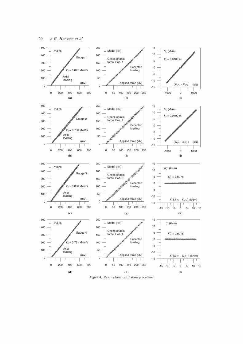
4. Load-cell performance

The load cells manufactured were calibrated in a Dartec 500 kN static testing machine using the

approach described above. The compressive load was applied cyclically at a frequency of 5 Hz.

The force level from the Dartec testing machine and the signal from the four strain gauges were

sampled digitally. All relevant data for one selected load cells is given in Figure 4. Figure 4(a–d)

give the relation between force level and signal from each strain gauge for pure-axial loading.

The relation is clearly linear although some hysteresis is evident from Gauge 2 and 3. The

hysteresis, or reversibility error, is the difference between the load cell�s output when a force has

been applied by monotonic increase from zero, and its output at the same force following a

monotonic decrease from its rated load (Robinson, 1997). Robinson (1997) gives four hysteresis

mechanisms for load cells. These are (1) metallurgical hysteresis, (2) local yielding effects,

(3) hysteresis in strain-gauge backing and adhesive layer and finally (4) slip at the interface

between load cell and support. Given the axissymmetry of the current load cell and support

conditions, hysteresis in the strain-gauge backing and adhesive layer could be a plausible

explanation for the hysteresis observed for Gauge 2 and 3 only. Four eccentric loading con-

ditions were applied to the load cell, namely loading by a steel ball through the four eccentrically

placed holes in the top flange, Figure 1. First, this load condition can be used to check the

performance of the calibration formula for the total axial force given by Eq. 2 and defined by

the constants Ki, i=1.4 of Figure 4(a–d). The results can be seen in Figure 4(e–h). The formulas

appear to give good results, although the force levels are somewhat underestimated by the

calibration formula for loading in Position 3 (which is the hole directly above Gauge 3). The


calibration results relating to the two bending moments Mx and My are shown in Figure 4(i–j).

The corresponding correction for the coupling error between the two bending moments is given

in Figure 4(k–l) and is less than 1% for both cases. The two load cells produced within this

project were calibrated and applied for impact testing of a bumper system. The dynamic results

followed by a discussion are reported by Hanssen et al. (2003).

5. Conclusions

A 3-component load cell for measurement of axial force and two orthogonal bending moments

has been developed for structural impact testing. The shape of the load cell was optimised by use

of finite element simulations. Finite element simulations were also carried out in order to study

the behaviour of the load cell for dynamic loading conditions. A simple set of calibration

formulas for the axial force and the bending moments was developed based on the assumption

of a linear and elastic strain distribution. Calibration of the load cell showed reasonable line-

arity. The load cell was subjected to eccentric loading conditions and the calibrated formula for

the axial force showed good consistency with the applied force levels.

References

Clough, R.W. and Penzien, J. (1975). Dynamics of Structures, McGraw Hill Company, Singapore, ISBN 0 07 085089 4.

Hallquist, J.O. (1998). Theoretical Manual, Livermore Software Technology Corporation, compiled by J.O. Hallquist.

Hanssen, A.G., Auestad, T., Tryland, T. and Langseth, M. (2003). The kicking machine: A device for impact testing of

structural components, International Journal of Crashworthiness 8(4), 385–392.

Jones, N. (1989). Structural Impact, Cambridge University Press. ISBN 0 521 30180 7.

Robinson, G.M. (1997). Finite element modeling of load cell hysteresis, Measurement 20(2), 103–107.
