CS559: Computer Graphics
Lecture 38: AnimationLi Zhang
Spring 2008
Slides from Brian Curless at U of Washington
Today• Computer Animation, Particle Systems
• Reading• (Optional) Shirley, ch 16, overview of animation
• Witkin, Particle System Dynamics, SIGGRAPH ’01 course notes on Physically Based Modeling.
• Witkin and Baraff, Differential Equation Basics, SIGGRAPH ’01 course notes on Physically Based Modeling.
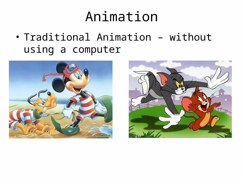
Animation• Traditional Animation – without using a computer
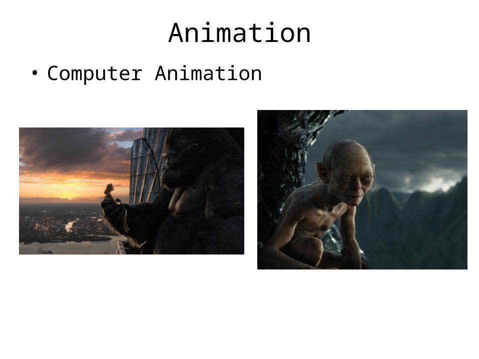
Animation• Computer Animation
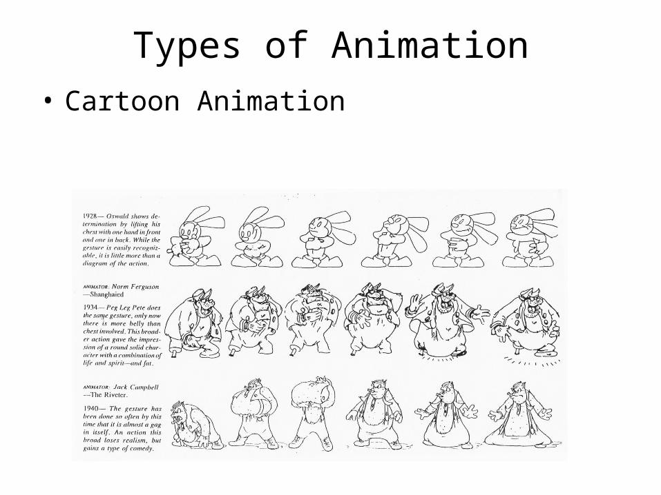
Types of Animation• Cartoon Animation
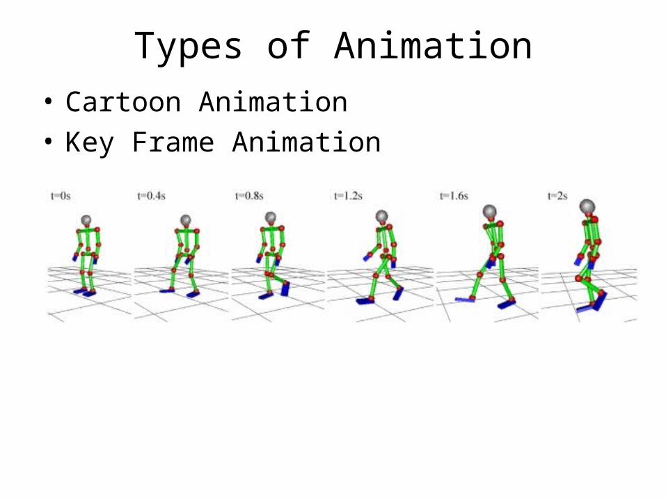
Types of Animation• Cartoon Animation• Key Frame Animation
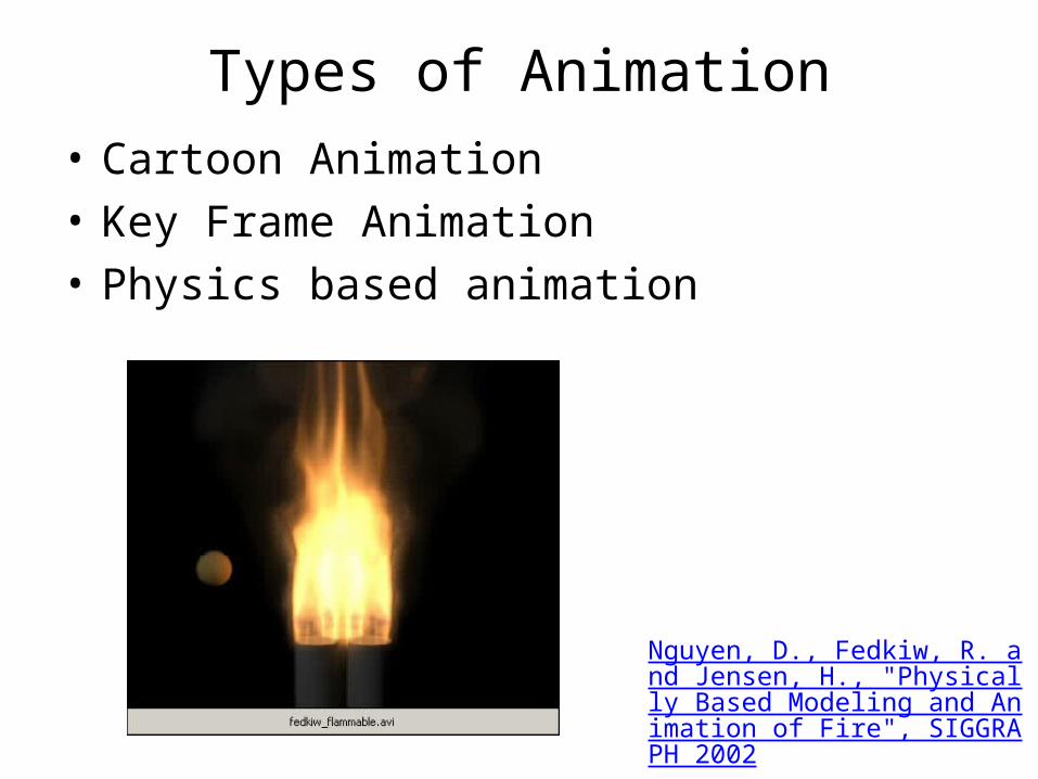
Types of Animation• Cartoon Animation• Key Frame Animation • Physics based animation
Nguyen, D., Fedkiw, R. and Jensen, H., "Physically Based Modeling and Animation of Fire", SIGGRAPH 2002
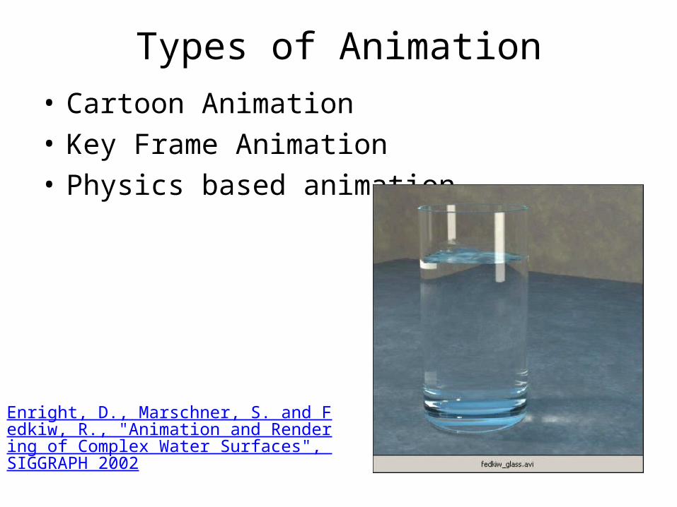
Types of Animation• Cartoon Animation• Key Frame Animation • Physics based animation
Enright, D., Marschner, S. and Fedkiw, R., "Animation and Rendering of Complex Water Surfaces", SIGGRAPH 2002
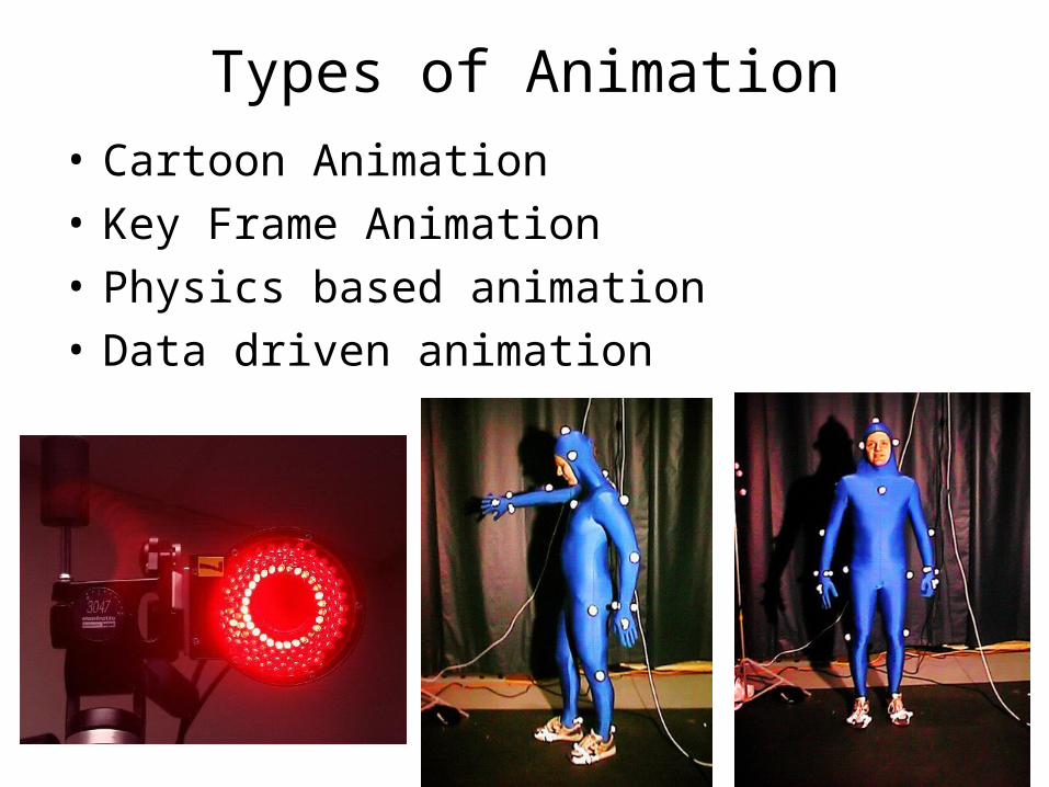
Types of Animation• Cartoon Animation• Key Frame Animation • Physics based animation• Data driven animation
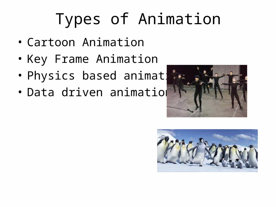
Types of Animation• Cartoon Animation• Key Frame Animation • Physics based animation• Data driven animation
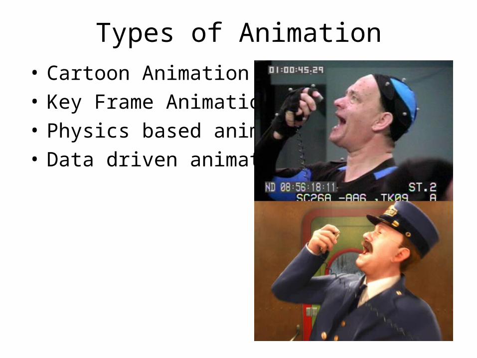
Types of Animation• Cartoon Animation• Key Frame Animation • Physics based animation• Data driven animation
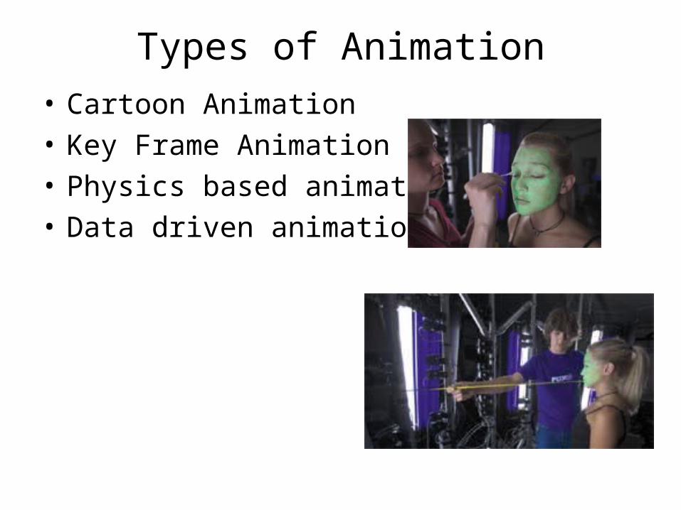
Types of Animation• Cartoon Animation• Key Frame Animation • Physics based animation• Data driven animation
Particle Systems• What are particle systems?
– A particle system is a collection of point masses that obeys some physical laws (e.g, gravity, heat convection, spring behaviors, …).
• Particle systems can be used to simulate all sorts of physical phenomena:
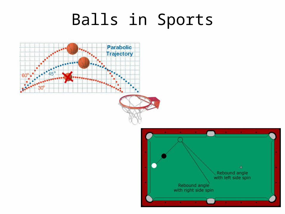
Balls in Sports
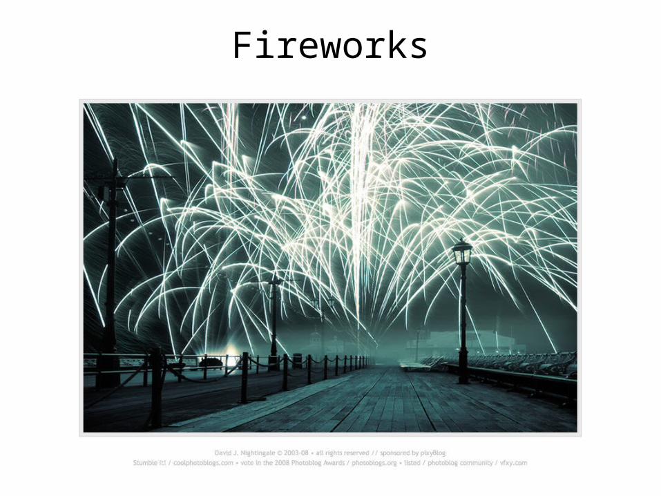
Fireworks
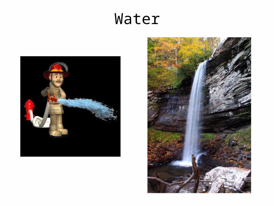
Water
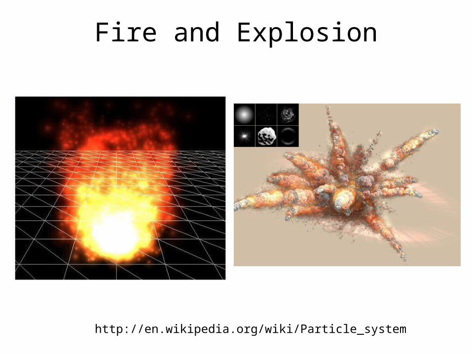
Fire and Explosion
http://en.wikipedia.org/wiki/Particle_system
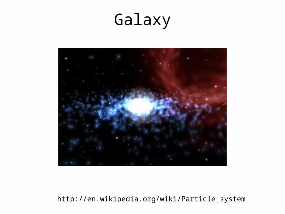
Galaxy
http://en.wikipedia.org/wiki/Particle_system
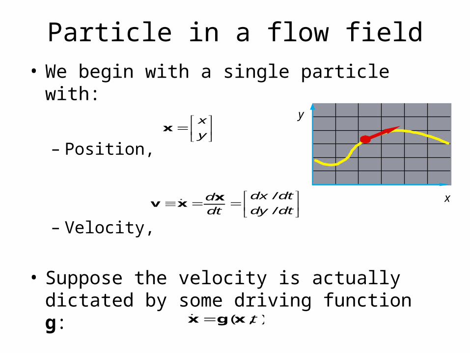
Particle in a flow field• We begin with a single particle with:
– Position,
– Velocity,
• Suppose the velocity is actually dictated by some driving function g:
( , )tx g x
/
/
dx dtddy dtdt
xv x
x
g(x,t)
x
yx
y
x
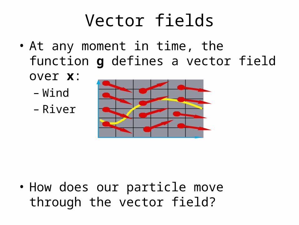
Vector fields• At any moment in time, the function g defines a
vector field over x:– Wind– River
• How does our particle move through the vector field?
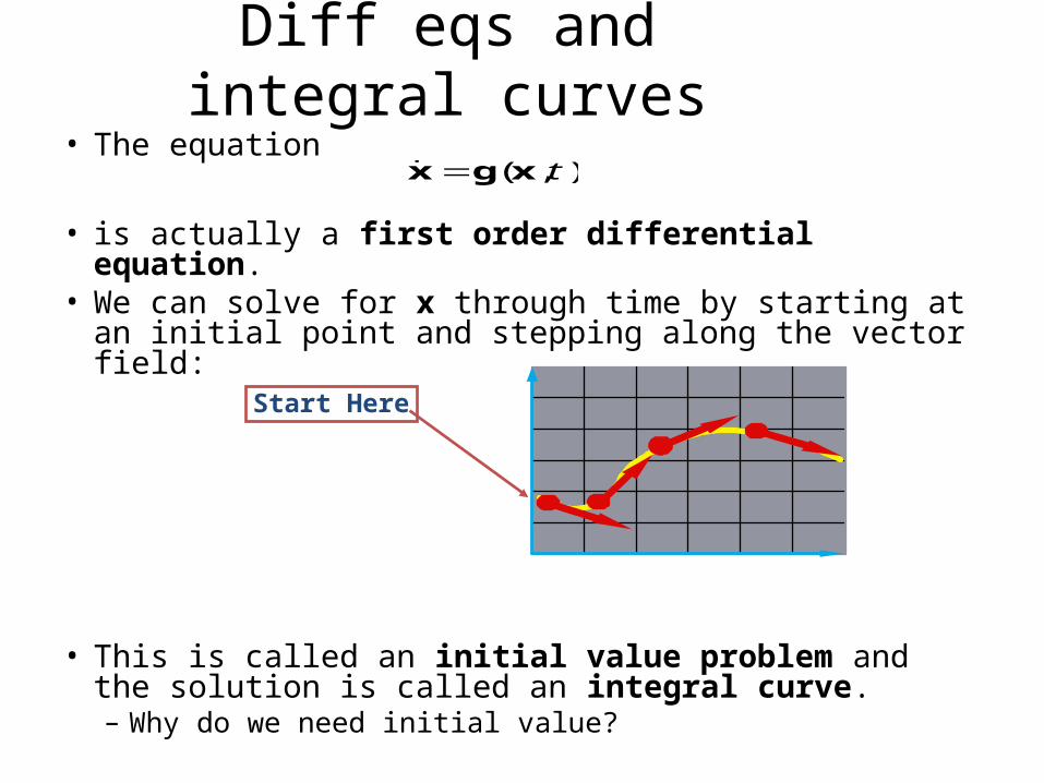
Diff eqs and integral curves• The equation
• is actually a first order differential equation.• We can solve for x through time by starting at an initial
point and stepping along the vector field:
• This is called an initial value problem and the solution is called an integral curve.– Why do we need initial value?
Start Here
( , )tx g x
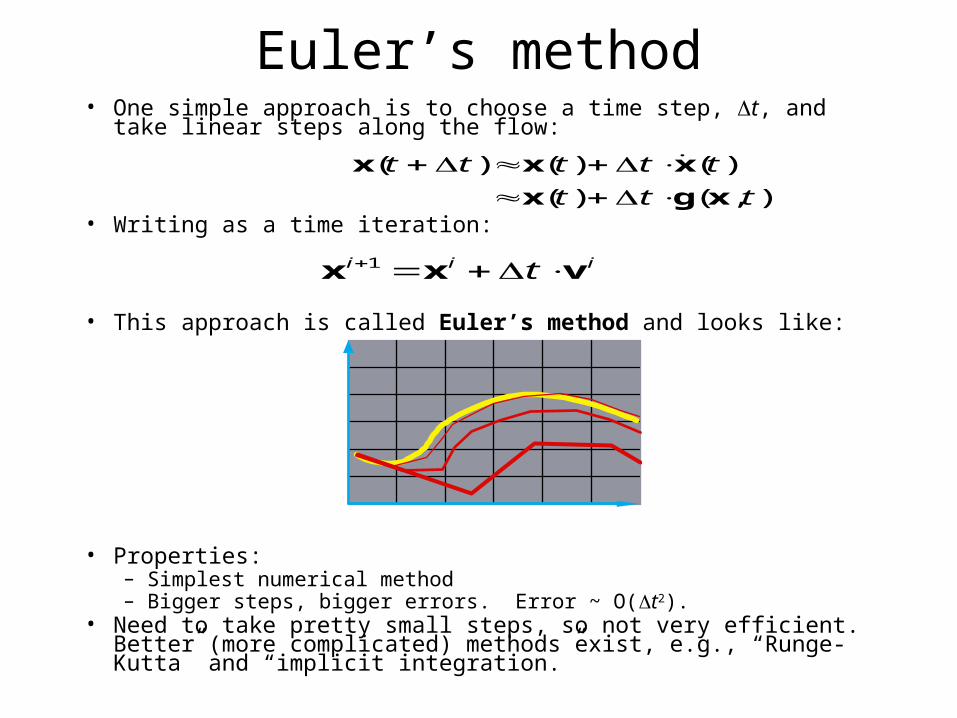
Euler’s method• One simple approach is to choose a time step, t, and take linear steps
along the flow:
• Writing as a time iteration:
• This approach is called Euler’s method and looks like:
• Properties:– Simplest numerical method– Bigger steps, bigger errors. Error ~ O(t2).
• Need to take pretty small steps, so not very efficient. Better (more complicated) methods exist, e.g., “Runge-Kutta” and “implicit integration.”
( ) ( ) ( )
( ) ( , )
t t t t t
t t t
x x x
x g x
1i i it x x v
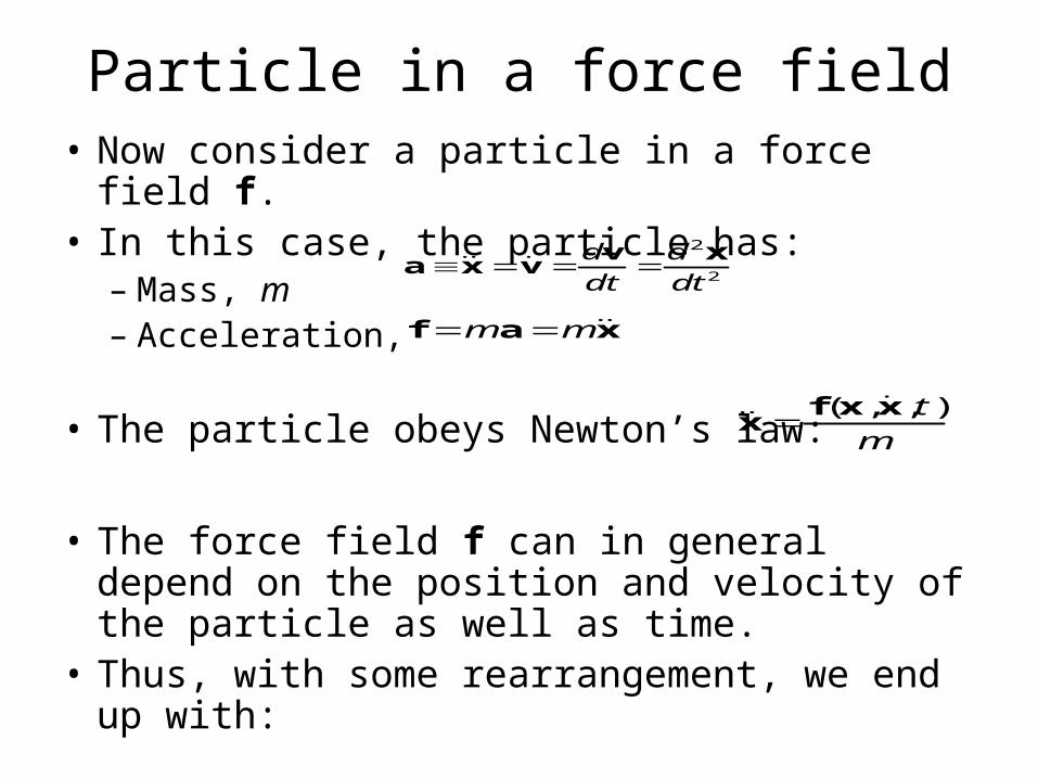
Particle in a force field• Now consider a particle in a force field f.• In this case, the particle has:
– Mass, m– Acceleration,
• The particle obeys Newton’s law:
• The force field f can in general depend on the position and velocity of the particle as well as time.
• Thus, with some rearrangement, we end up with:
( , , )tm
f x x
x
m m f a x
2
2d ddt dtv
a x vx
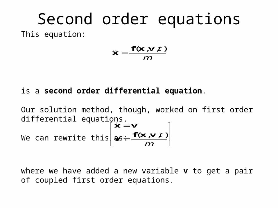
This equation:
is a second order differential equation.
Our solution method, though, worked on first order differential equations.
We can rewrite this as:
where we have added a new variable v to get a pair of coupled first order equations.
Second order equations
( , , )tm
x v
f x vv
( , , )tm
f x v
x

Phase space
• Concatenate x and v to make a 6-vector: position in phase space.
• Taking the time derivative: another 6-vector.
• A vanilla 1st-order differential equation.
x
v
/m
x v
v f
x
v
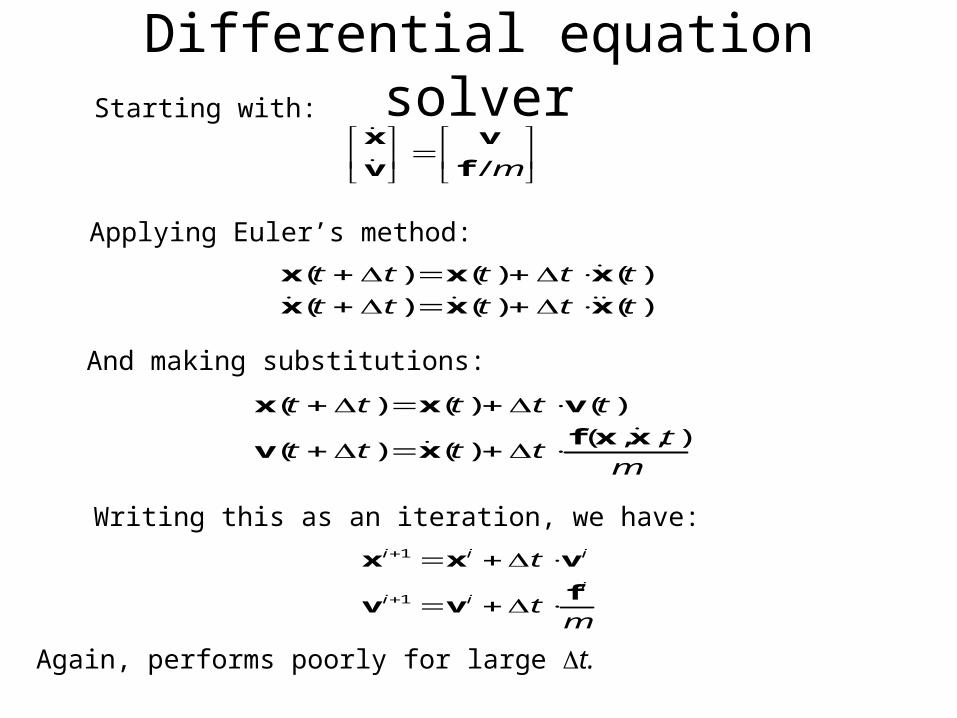
Differential equation solver
Applying Euler’s method:
( ) ( ) ( )
( ) ( ) ( )
t t t t t
t t t t t
x x x
x x x
Again, performs poorly for large t.
/m
x v
v f
1
1
i i i
ii i
t
tm
x x v
fv v
( ) ( ) ( )
( , , )( ) ( )
t t t t t
tt t t t
m
x x v
f x xv x
And making substitutions:
Writing this as an iteration, we have:
Starting with:
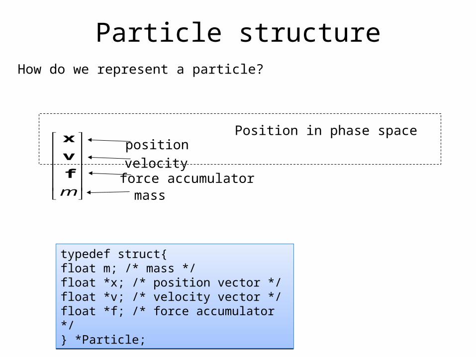
Particle structure
m
x
v
f
positionvelocityforce accumulatormass
Position in phase space
How do we represent a particle?
typedef struct{float m; /* mass */float *x; /* position vector */float *v; /* velocity vector */float *f; /* force accumulator */} *Particle;
typedef struct{float m; /* mass */float *x; /* position vector */float *v; /* velocity vector */float *f; /* force accumulator */} *Particle;
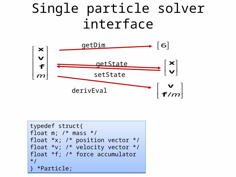
Single particle solver interface
m
x
v
f
x
v
/m
v
f
6getDim
derivEval
getState
setState
typedef struct{float m; /* mass */float *x; /* position vector */float *v; /* velocity vector */float *f; /* force accumulator */} *Particle;
typedef struct{float m; /* mass */float *x; /* position vector */float *v; /* velocity vector */float *f; /* force accumulator */} *Particle;
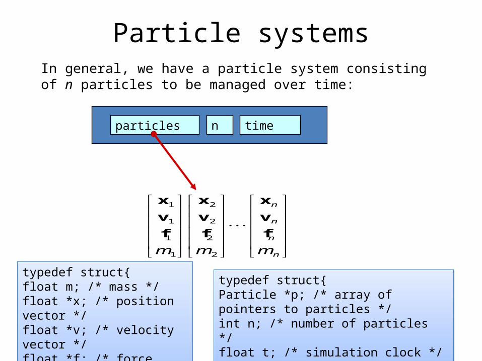
Particle systems
particles n time
In general, we have a particle system consisting of n particles to be managed over time:
1 2
1 2
1 2
1 2
n
n
n
nm m m
x x x
v v v
ff f
typedef struct{Particle *p; /* array of pointers to particles */int n; /* number of particles */float t; /* simulation clock */} *ParticleSystem
typedef struct{Particle *p; /* array of pointers to particles */int n; /* number of particles */float t; /* simulation clock */} *ParticleSystem
typedef struct{float m; /* mass */float *x; /* position vector */float *v; /* velocity vector */float *f; /* force accumulator */} *Particle;
typedef struct{float m; /* mass */float *x; /* position vector */float *v; /* velocity vector */float *f; /* force accumulator */} *Particle;
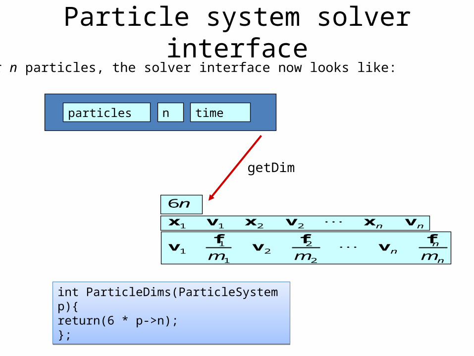
Particle system solver interface
particles n time
1 1 2 2
1 21 2
1 2
6
n n
nn
n
n
m m m
x v x v x v
ff fv v v
getDim
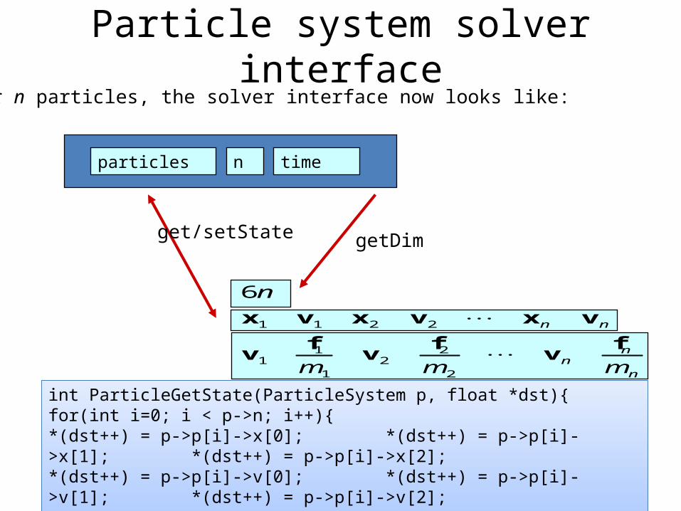
For n particles, the solver interface now looks like:
int ParticleDims(ParticleSystem p){return(6 * p->n);};
int ParticleDims(ParticleSystem p){return(6 * p->n);};
Particle system solver interface
particles n time
1 1 2 2
1 21 2
1 2
6
n n
nn
n
n
m m m
x v x v x v
ff fv v v
get/setState getDim
For n particles, the solver interface now looks like:
int ParticleGetState(ParticleSystem p, float *dst){for(int i=0; i < p->n; i++){*(dst++) = p->p[i]->x[0]; *(dst++) = p->p[i]->x[1]; *(dst++) = p->p[i]->x[2];*(dst++) = p->p[i]->v[0]; *(dst++) = p->p[i]->v[1]; *(dst++) = p->p[i]->v[2];}}
int ParticleGetState(ParticleSystem p, float *dst){for(int i=0; i < p->n; i++){*(dst++) = p->p[i]->x[0]; *(dst++) = p->p[i]->x[1]; *(dst++) = p->p[i]->x[2];*(dst++) = p->p[i]->v[0]; *(dst++) = p->p[i]->v[1]; *(dst++) = p->p[i]->v[2];}}
Particle system solver interface
particles n time
1 1 2 2
1 21 2
1 2
6
n n
nn
n
n
m m m
x v x v x v
ff fv v v
derivEval
get/setState getDim
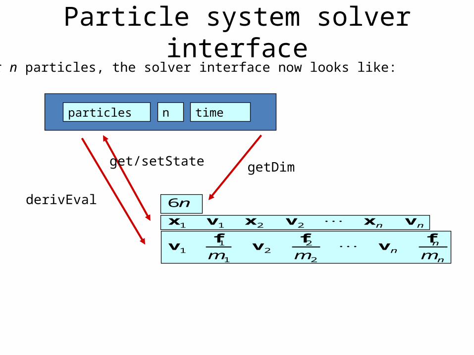
For n particles, the solver interface now looks like:

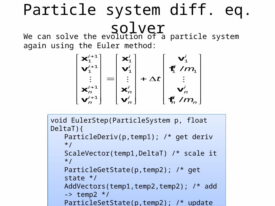
Particle system diff. eq. solverWe can solve the evolution of a particle system again using the Euler method:
11 1 1
11 1 1 1
1
1
/
/
i i i
i i i
i i in n ni i in n n n
mt
m
x x v
v v f
x x v
v v f
void EulerStep(ParticleSystem p, float DeltaT){ParticleDeriv(p,temp1); /* get deriv */ScaleVector(temp1,DeltaT) /* scale it */ParticleGetState(p,temp2); /* get state */AddVectors(temp1,temp2,temp2); /* add -> temp2 */ParticleSetState(p,temp2); /* update state */p->t += DeltaT; /* update time */
}
void EulerStep(ParticleSystem p, float DeltaT){ParticleDeriv(p,temp1); /* get deriv */ScaleVector(temp1,DeltaT) /* scale it */ParticleGetState(p,temp2); /* get state */AddVectors(temp1,temp2,temp2); /* add -> temp2 */ParticleSetState(p,temp2); /* update state */p->t += DeltaT; /* update time */
}
Forces• Each particle can experience a force which sends
it on its merry way.• Where do these forces come from? Some
examples:– Constant (gravity)– Position/time dependent (force fields)– Velocity-dependent (drag)– N-ary (springs)
• How do we compute the net force on a particle?
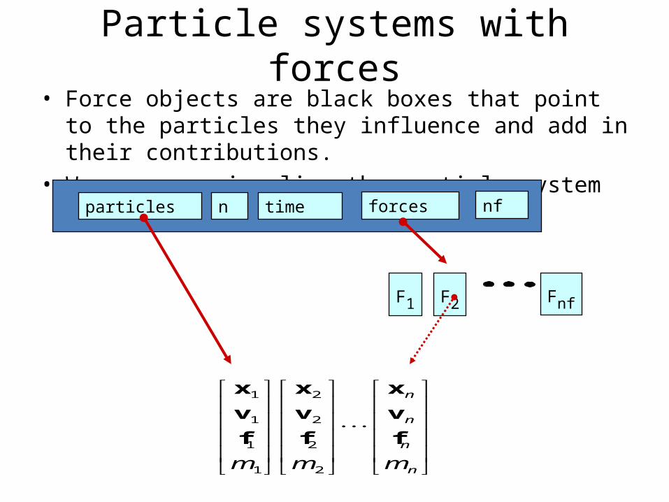
• Force objects are black boxes that point to the particles they influence and add in their contributions.
• We can now visualize the particle system with force objects:
Particle systems with forces
particles n time forces
F2 Fnf
nf
1 2
1 2
1 2
1 2
n
n
n
nm m m
x x x
v v v
ff f
F1
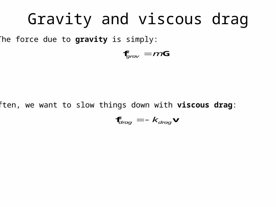
Gravity and viscous drag
grav mf G
drag dragkf v
The force due to gravity is simply:
Often, we want to slow things down with viscous drag:
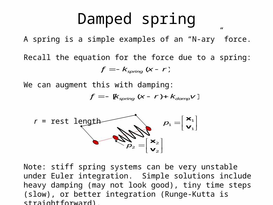
A spring is a simple examples of an “N-ary” force.
Recall the equation for the force due to a spring:
We can augment this with damping:
Note: stiff spring systems can be very unstable under Euler integration. Simple solutions include heavy damping (may not look good), tiny time steps (slow), or better integration (Runge-Kutta is straightforward).
Damped spring
( )springf k x r
[ ( ) ]spring dampf k x r k v
r = rest length 11
1
p
x
v
22
2
p
x
v
1 2
1 2
1 2
1 2
0 0 0
n
n
n
nm m m
x x x
v v v
ff f
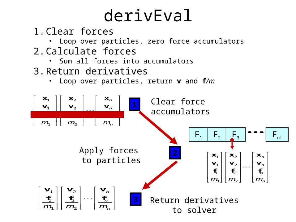
derivEval1. Clear forces
• Loop over particles, zero force accumulators
2. Calculate forces• Sum all forces into accumulators
3. Return derivatives• Loop over particles, return v and f/m
1 2
1 2
1 2
n
n
nm m m
v v v
ff f
Apply forces to particles
Clear force accumulators
1
2
3 Return derivativesto solver
1 2
1 2
1 2
1 2
n
n
n
nm m m
x x x
v v v
ff f
F2 F3 FnfF1
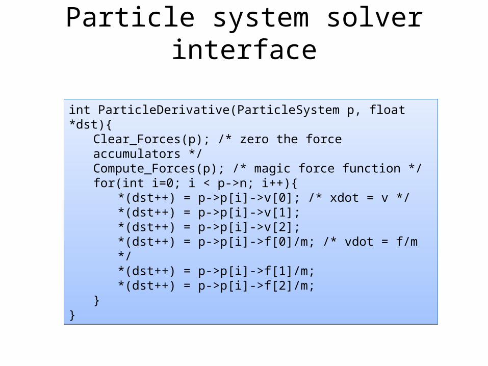
Particle system solver interface
int ParticleDerivative(ParticleSystem p, float *dst){Clear_Forces(p); /* zero the force accumulators */Compute_Forces(p); /* magic force function */for(int i=0; i < p->n; i++){
*(dst++) = p->p[i]->v[0]; /* xdot = v */*(dst++) = p->p[i]->v[1];*(dst++) = p->p[i]->v[2];*(dst++) = p->p[i]->f[0]/m; /* vdot = f/m */*(dst++) = p->p[i]->f[1]/m;*(dst++) = p->p[i]->f[2]/m;
}}
Particle system diff. eq. solverWe can solve the evolution of a particle system again using the Euler method:
11 1 1
11 1 1 1
1
1
/
/
i i i
i i i
i i in n ni i in n n n
mt
m
x x v
v v f
x x v
v v f
void EulerStep(ParticleSystem p, float DeltaT){ParticleDeriv(p,temp1); /* get deriv */ScaleVector(temp1,DeltaT) /* scale it */ParticleGetState(p,temp2); /* get state */AddVectors(temp1,temp2,temp2); /* add -> temp2 */ParticleSetState(p,temp2); /* update state */p->t += DeltaT; /* update time */
}
void EulerStep(ParticleSystem p, float DeltaT){ParticleDeriv(p,temp1); /* get deriv */ScaleVector(temp1,DeltaT) /* scale it */ParticleGetState(p,temp2); /* get state */AddVectors(temp1,temp2,temp2); /* add -> temp2 */ParticleSetState(p,temp2); /* update state */p->t += DeltaT; /* update time */
}
Recommended