CS252Graduate Computer Architecture
Lecture 13
Vector Processing (Con’t)Intro to Multiprocessing
March 7th, 2011
John Kubiatowicz
Electrical Engineering and Computer Sciences
University of California, Berkeley
http://www.eecs.berkeley.edu/~kubitron/cs252
3/7/2011 cs252-S11, Lecture 13 2
+ + + + + +
[0] [1] [VLR-1]
Vector Arithmetic Instructions
ADDV v3, v1, v2 v3
v2v1
Scalar Registers
r0
r15Vector Registers
v0
v15
[0] [1] [2] [VLRMAX-1]
VLRVector Length Register
v1Vector Load and
Store Instructions
LV v1, r1, r2
Base, r1 Stride, r2Memory
Vector Register
Recall: Vector Programming Model
3/7/2011 cs252-S11, Lecture 13 3
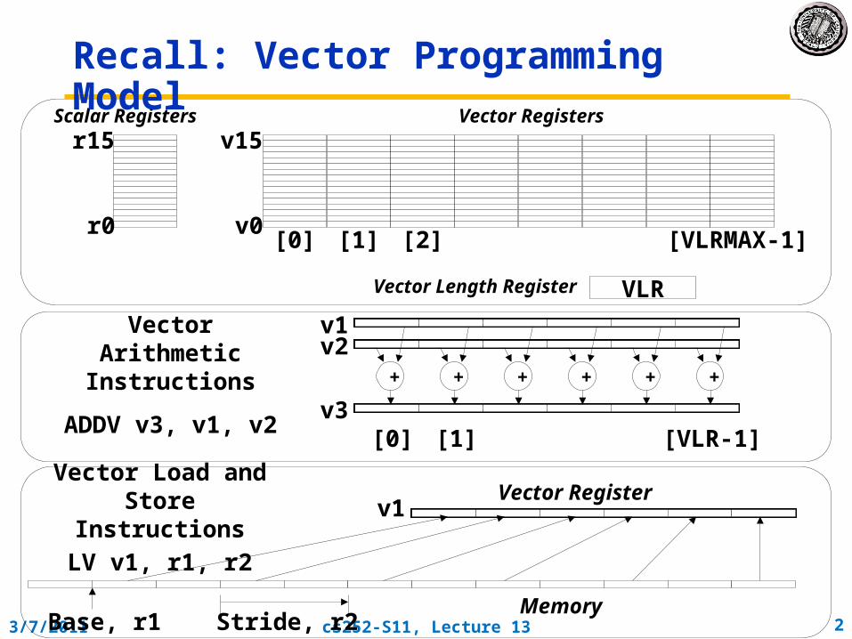
Vector Code Example
# Scalar Code LI R4, 64loop: L.D F0, 0(R1) L.D F2, 0(R2) ADD.D F4, F2, F0 S.D F4, 0(R3) DADDIU R1, 8 DADDIU R2, 8 DADDIU R3, 8 DSUBIU R4, 1 BNEZ R4, loop
# Vector Code LI VLR, 64 LV V1, R1 LV V2, R2 ADDV.D V3, V1, V2 SV V3, R3
# C codefor (i=0; i<64; i++) C[i] = A[i] + B[i];

3/7/2011 cs252-S11, Lecture 13 4
Vector Instruction Set Advantages
• Compact– one short instruction encodes N operations
• Expressive, tells hardware that these N operations:– are independent
– use the same functional unit
– access disjoint registers
– access registers in the same pattern as previous instructions
– access a contiguous block of memory (unit-stride load/store)
– access memory in a known pattern (strided load/store)
• Scalable– can run same object code on more parallel pipelines or lanes
3/7/2011 cs252-S11, Lecture 13 5
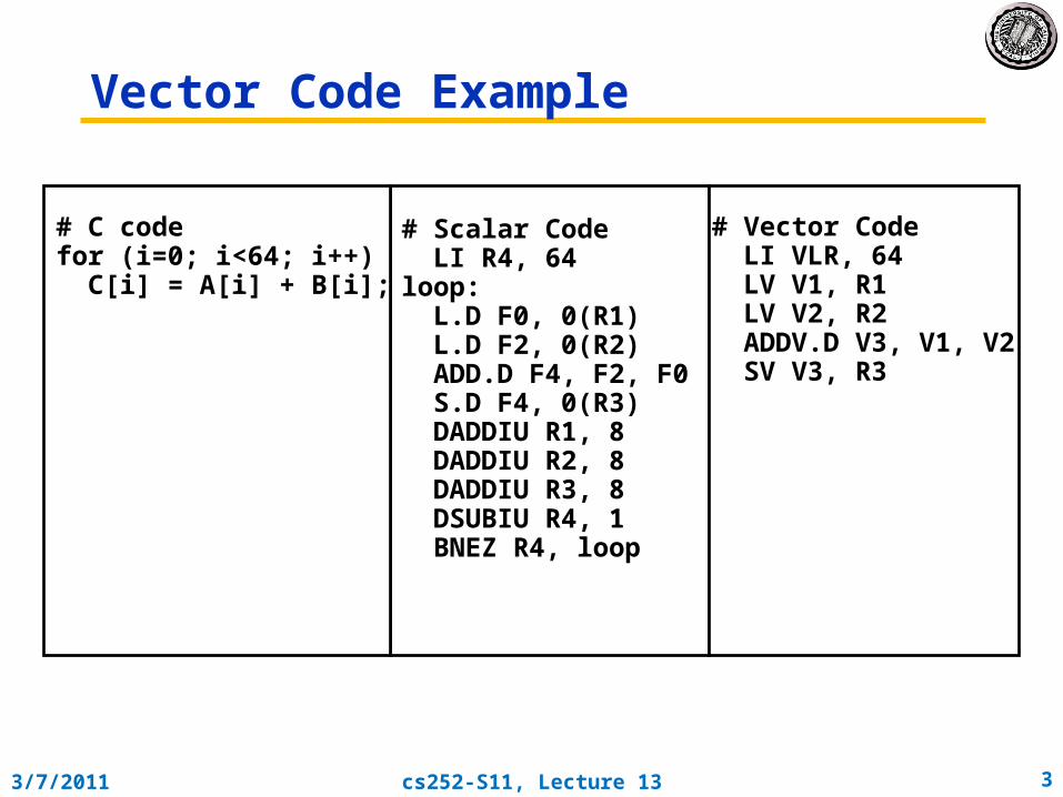
V1
V2
V3
•V3 <- v1 * v2
•Six stage multiply pipeline
• Use deep pipeline (=> fast clock) to execute element operations
• Simplifies control of deep pipeline because elements in vector are independent (=> no hazards!)
Vector Arithmetic Execution

3/7/2011 cs252-S11, Lecture 13 6
Vector Instruction ExecutionADDV C,A,B
C[1]
C[2]
C[0]
A[3] B[3]
A[4] B[4]
A[5] B[5]
A[6] B[6]
Execution using one pipelined functional unit
C[4]
C[8]
C[0]
A[12] B[12]
A[16] B[16]
A[20] B[20]
A[24] B[24]
C[5]
C[9]
C[1]
A[13] B[13]
A[17] B[17]
A[21] B[21]
A[25] B[25]
C[6]
C[10]
C[2]
A[14] B[14]
A[18] B[18]
A[22] B[22]
A[26] B[26]
C[7]
C[11]
C[3]
A[15] B[15]
A[19] B[19]
A[23] B[23]
A[27] B[27]
Execution using four pipelined functional units

3/7/2011 cs252-S11, Lecture 13 7
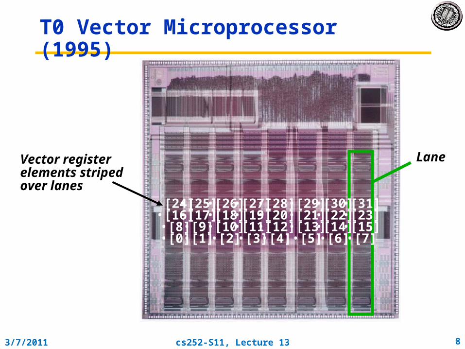
Vector Unit Structure
•Lane
•Functional Unit
VectorRegisters
Memory Subsystem
Elements 0, 4, 8, …
Elements 1, 5, 9, …
Elements 2, 6, 10, …
Elements 3, 7, 11, …
3/7/2011 cs252-S11, Lecture 13 8
T0 Vector Microprocessor (1995)
LaneVector register elements striped over lanes
•[0]•[8]
•[16]•[24]
•[1]•[9]
•[17]•[25]
•[2]•[10]•[18]•[26]
•[3]•[11]•[19]•[27]
•[4]•[12]•[20]•[28]
•[5]•[13]•[21]•[29]
•[6]•[14]•[22]•[30]
•[7]•[15]•[23]•[31]

3/7/2011 cs252-S11, Lecture 13 9
Vector Memory-Memory vs.Vector Register Machines
• Vector memory-memory instructions hold all vector operands in main memory
• The first vector machines, CDC Star-100 (‘73) and TI ASC (‘71), were memory-memory machines
• Cray-1 (’76) was first vector register machine
for (i=0; i<N; i++)
{
C[i] = A[i] + B[i];
D[i] = A[i] - B[i];
}
Example Source Code ADDV C, A, B
SUBV D, A, B
Vector Memory-Memory Code
LV V1, A
LV V2, B
ADDV V3, V1, V2
SV V3, C
SUBV V4, V1, V2
SV V4, D
Vector Register Code

3/7/2011 cs252-S11, Lecture 13 10
Vector Memory-Memory vs. Vector Register Machines
• Vector memory-memory architectures (VMMA) require greater main memory bandwidth, why?
– All operands must be read in and out of memory• VMMAs make if difficult to overlap execution of
multiple vector operations, why? – Must check dependencies on memory addresses
• VMMAs incur greater startup latency– Scalar code was faster on CDC Star-100 for vectors < 100
elements– For Cray-1, vector/scalar breakeven point was around 2
elementsApart from CDC follow-ons (Cyber-205, ETA-10) all
major vector machines since Cray-1 have had vector register architectures
(we ignore vector memory-memory from now on)
3/7/2011 cs252-S11, Lecture 13 11
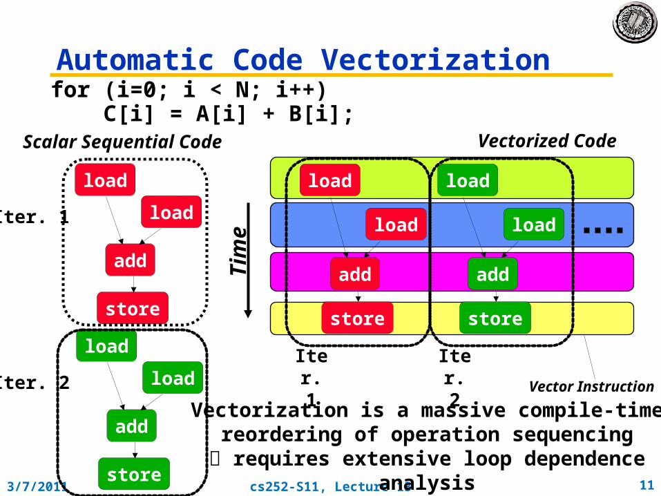
Automatic Code Vectorizationfor (i=0; i < N; i++) C[i] = A[i] + B[i];
load
load
add
store
load
load
add
store
Iter. 1
Iter. 2
Scalar Sequential Code
Vectorization is a massive compile-time reordering of operation sequencing
requires extensive loop dependence analysis
Vector Instruction
load
load
add
store
load
load
add
store
Iter. 1
Iter. 2
Vectorized Code
Tim
e

3/7/2011 cs252-S11, Lecture 13 12
Vector StripminingProblem: Vector registers have finite lengthSolution: Break loops into pieces that fit into vector
registers, “Stripmining” ANDI R1, N, 63 # N mod 64 MTC1 VLR, R1 # Do remainderloop: LV V1, RA DSLL R2, R1, 3 # Multiply by 8 DADDU RA, RA, R2 # Bump pointer LV V2, RB DADDU RB, RB, R2 ADDV.D V3, V1, V2 SV V3, RC DADDU RC, RC, R2 DSUBU N, N, R1 # Subtract elements LI R1, 64 MTC1 VLR, R1 # Reset full length BGTZ N, loop # Any more to do?
for (i=0; i<N; i++) C[i] = A[i]+B[i];
+
+
+
A B C
64 elements
Remainder
•3/7/2011 •cs252-S11, Lecture 13 •1332
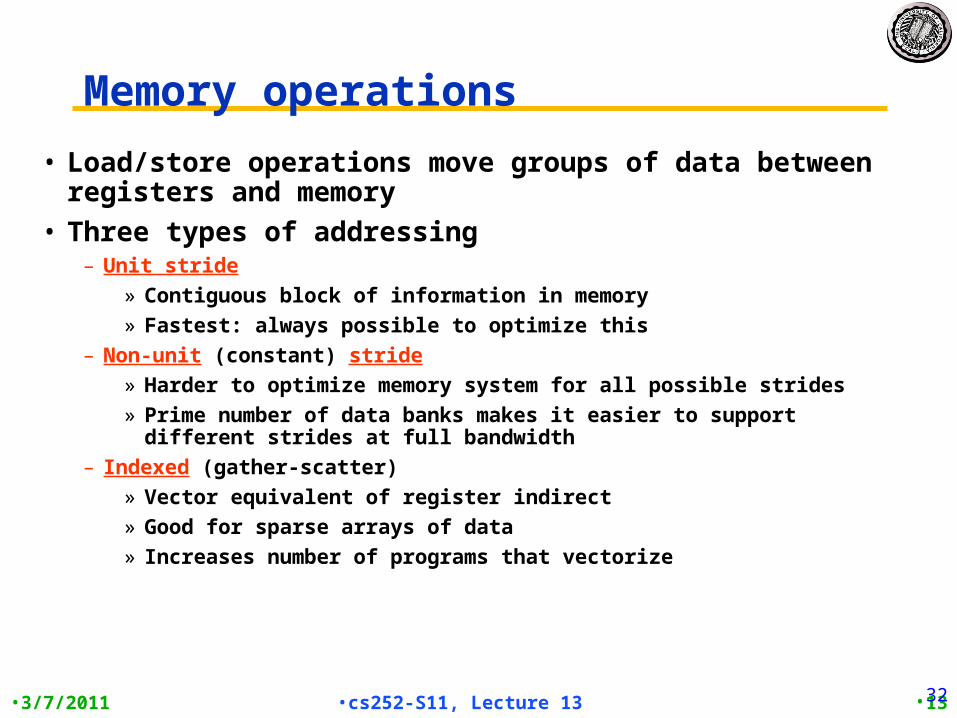
Memory operations
• Load/store operations move groups of data between registers and memory
• Three types of addressing– Unit stride
» Contiguous block of information in memory
» Fastest: always possible to optimize this
– Non-unit (constant) stride
» Harder to optimize memory system for all possible strides
» Prime number of data banks makes it easier to support different strides at full bandwidth
– Indexed (gather-scatter)
» Vector equivalent of register indirect
» Good for sparse arrays of data
» Increases number of programs that vectorize
•3/7/2011 •cs252-S11, Lecture 13 •14
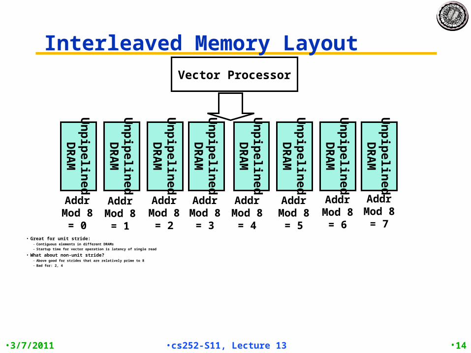
Interleaved Memory Layout
• Great for unit stride: – Contiguous elements in different DRAMs– Startup time for vector operation is latency of single read
• What about non-unit stride?– Above good for strides that are relatively prime to 8– Bad for: 2, 4
Vector Processor
Un
pip
elin
ed
DR
AM
Un
pip
elin
ed
DR
AM
Un
pip
elin
ed
DR
AM
Un
pip
elin
ed
DR
AM
Un
pip
elin
ed
DR
AM
Un
pip
elin
ed
DR
AM
Un
pip
elin
ed
DR
AM
Un
pip
elin
ed
DR
AM
AddrMod 8
= 0
AddrMod 8
= 1
AddrMod 8
= 2
AddrMod 8
= 4
AddrMod 8
= 5
AddrMod 8
= 3
AddrMod 8
= 6
AddrMod 8
= 7

•3/7/2011 •cs252-S11, Lecture 13 •15
How to get full bandwidth for Unit Stride?• Memory system must sustain (# lanes x word) /clock
• No. memory banks > memory latency to avoid stalls– m banks m words per memory lantecy l clocks
– if m < l, then gap in memory pipeline:
clock: 0 … l l+1 l+2 … l+m- 1 l+m …2 l
word: -- … 0 1 2 … m-1 -- …m– may have 1024 banks in SRAM
• If desired throughput greater than one word per cycle– Either more banks (start multiple requests simultaneously)
– Or wider DRAMS. Only good for unit stride or large data types
• More banks/weird numbers of banks good to support more strides at full bandwidth
– can read paper on how to do prime number of banks efficiently
•3/7/2011 •cs252-S11, Lecture 13 •16
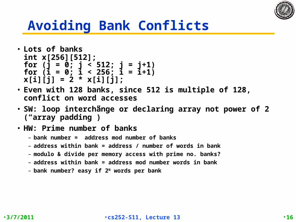
Avoiding Bank Conflicts
• Lots of banksint x[256][512];
for (j = 0; j < 512; j = j+1)for (i = 0; i < 256; i = i+1)
x[i][j] = 2 * x[i][j];• Even with 128 banks, since 512 is multiple of 128, conflict on word
accesses
• SW: loop interchange or declaring array not power of 2 (“array padding”)
• HW: Prime number of banks– bank number = address mod number of banks
– address within bank = address / number of words in bank
– modulo & divide per memory access with prime no. banks?
– address within bank = address mod number words in bank
– bank number? easy if 2N words per bank

3/7/2011 cs252-S11, Lecture 13 17
Finding Bank Number and Address within a bank
• Problem: Determine the number of banks, Nb and the number of words in each bank, Nw, such that:
– given address x, it is easy to find the bank where x will be found, B(x), and the address of x within the bank, A(x).
– for any address x, B(x) and A(x) are unique– the number of bank conflicts is minimized
• Solution: Use the Chinese remainder theorem to determine B(x) and A(x):B(x) = x MOD Nb
A(x) = x MOD Nw where Nb and Nw are co-prime (no factors)
– Chinese Remainder Theorem shows that B(x) and A(x) unique.
• Condition allows Nw to be power of two (typical) if Nb is prime of form 2m-1.
• Simple (fast) circuit to compute (x mod Nb) when Nb = 2m-1:– Since 2k
= 2k-m (2m-1) + 2k-m
2k MOD Nb = 2k-m MOD Nb =…= 2j with j< m– And, remember that: (A+B) MOD C = [(A MOD C)+(B MOD C)] MOD C– for every power of 2, compute single bit MOD (in advance)
– B(x) = sum of these values MOD Nb (low complexity circuit, adder with ~ m bits)

3/7/2011 cs252-S11, Lecture 13 18
Administrivia• Exam: Wednesday 3/30
Location: 320 SodaTIME: 2:30-5:30
– This info is on the Lecture page (has been)
– Get on 8 ½ by 11 sheet of notes (both sides)
– Meet at LaVal’s afterwards for Pizza and Beverages
• CS252 First Project proposal due by Friday 3/4– Need two people/project (although can justify three for right
project)
– Complete Research project in 9 weeks» Typically investigate hypothesis by building an artifact and
measuring it against a “base case”
» Generate conference-length paper/give oral presentation
» Often, can lead to an actual publication.

3/7/2011 cs252-S11, Lecture 13 19
load
Vector Instruction ParallelismCan overlap execution of multiple vector instructions– example machine has 32 elements per vector register and
8 lanes
loadmul
mul
add
add
Load Unit Multiply Unit Add Unit
time
Instruction issue
Complete 24 operations/cycle while issuing 1 short instruction/cycle

3/7/2011 cs252-S11, Lecture 13 20
Vector Chaining• Vector version of register bypassing
– introduced with Cray-1
Memory
V1
Load Unit
Mult.
V2
V3
Chain
Add
V4
V5
Chain
LV v1
MULV v3,v1,v2
ADDV v5, v3, v4

3/7/2011 cs252-S11, Lecture 13 21
Vector Chaining Advantage
• With chaining, can start dependent instruction as soon as first result appears
Load
Mul
Add
Load
Mul
AddTime
• Without chaining, must wait for last element of result to be written before starting dependent instruction

3/7/2011 cs252-S11, Lecture 13 22
Vector StartupTwo components of vector startup penalty
– functional unit latency (time through pipeline)
– dead time or recovery time (time before another vector instruction can start down pipeline)
R X X X W
R X X X W
R X X X W
R X X X W
R X X X W
R X X X W
R X X X W
R X X X W
R X X X W
R X X X W
Functional Unit Latency
Dead Time
First Vector Instruction
Second Vector Instruction
Dead Time

3/7/2011 cs252-S11, Lecture 13 23
Dead Time and Short Vectors
Cray C90, Two lanes
4 cycle dead time
Maximum efficiency 94% with 128 element vectors
4 cycles dead time T0, Eight lanes
No dead time
100% efficiency with 8 element vectors
No dead time
64 cycles active
3/7/2011 cs252-S11, Lecture 13 24
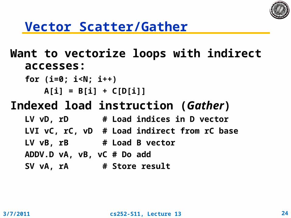
Vector Scatter/Gather
Want to vectorize loops with indirect accesses:for (i=0; i<N; i++)
A[i] = B[i] + C[D[i]]
Indexed load instruction (Gather)LV vD, rD # Load indices in D vector
LVI vC, rC, vD # Load indirect from rC base
LV vB, rB # Load B vector
ADDV.D vA, vB, vC # Do add
SV vA, rA # Store result
3/7/2011 cs252-S11, Lecture 13 25
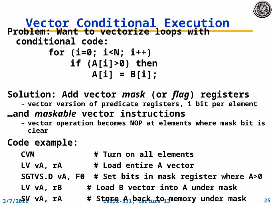
Vector Conditional ExecutionProblem: Want to vectorize loops with conditional code:
for (i=0; i<N; i++) if (A[i]>0) then A[i] = B[i];
Solution: Add vector mask (or flag) registers– vector version of predicate registers, 1 bit per element
…and maskable vector instructions– vector operation becomes NOP at elements where mask bit is clear
Code example:CVM # Turn on all elements
LV vA, rA # Load entire A vector
SGTVS.D vA, F0 # Set bits in mask register where A>0
LV vA, rB # Load B vector into A under mask
SV vA, rA # Store A back to memory under mask
3/7/2011 cs252-S11, Lecture 13 26
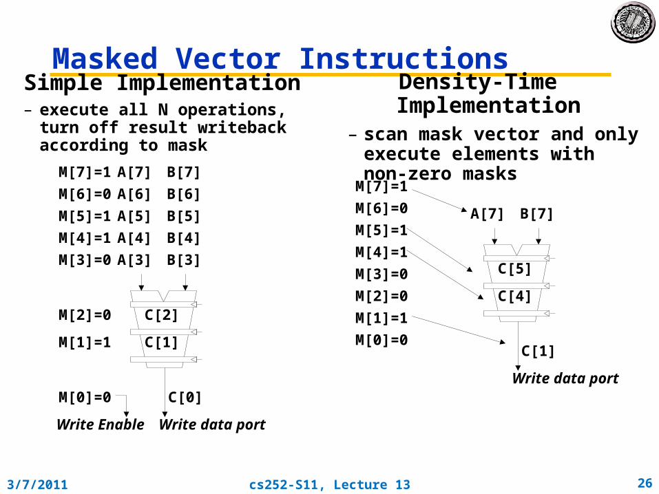
Masked Vector Instructions
C[4]
C[5]
C[1]
Write data port
A[7] B[7]
M[3]=0
M[4]=1
M[5]=1
M[6]=0
M[2]=0
M[1]=1
M[0]=0
M[7]=1
Density-Time Implementation– scan mask vector and only
execute elements with non-zero masks
C[1]
C[2]
C[0]
A[3] B[3]
A[4] B[4]
A[5] B[5]
A[6] B[6]
M[3]=0
M[4]=1
M[5]=1
M[6]=0
M[2]=0
M[1]=1
M[0]=0
Write data portWrite Enable
A[7] B[7]M[7]=1
Simple Implementation– execute all N operations, turn off
result writeback according to mask

3/7/2011 cs252-S11, Lecture 13 27
Compress/Expand Operations• Compress packs non-masked elements from one
vector register contiguously at start of destination vector register
– population count of mask vector gives packed vector length
• Expand performs inverse operation
M[3]=0
M[4]=1
M[5]=1
M[6]=0
M[2]=0
M[1]=1
M[0]=0
M[7]=1
A[3]
A[4]
A[5]
A[6]
A[7]
A[0]
A[1]
A[2]
M[3]=0
M[4]=1
M[5]=1
M[6]=0
M[2]=0
M[1]=1
M[0]=0
M[7]=1
B[3]
A[4]
A[5]
B[6]
A[7]
B[0]
A[1]
B[2]
Expand
A[7]
A[1]
A[4]
A[5]
Compress
A[7]
A[1]
A[4]
A[5]
Used for density-time conditionals and also for general selection operations
3/7/2011 cs252-S11, Lecture 13 28
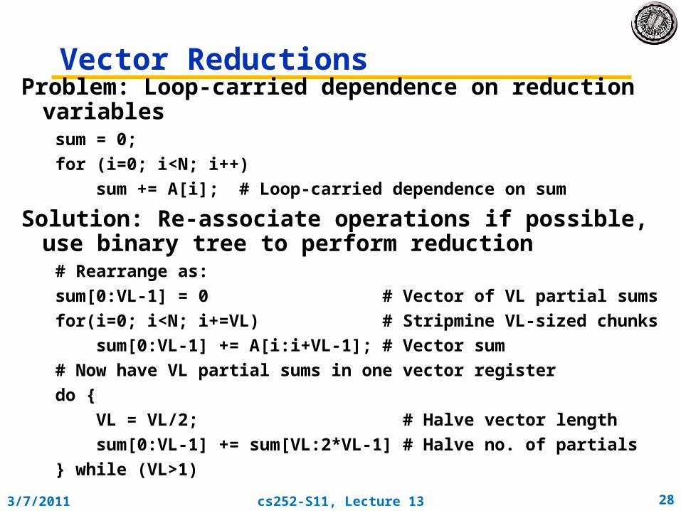
Vector ReductionsProblem: Loop-carried dependence on reduction variables
sum = 0;
for (i=0; i<N; i++)
sum += A[i]; # Loop-carried dependence on sum
Solution: Re-associate operations if possible, use binary tree to perform reduction# Rearrange as:
sum[0:VL-1] = 0 # Vector of VL partial sums
for(i=0; i<N; i+=VL) # Stripmine VL-sized chunks
sum[0:VL-1] += A[i:i+VL-1]; # Vector sum
# Now have VL partial sums in one vector register
do {
VL = VL/2; # Halve vector length
sum[0:VL-1] += sum[VL:2*VL-1] # Halve no. of partials
} while (VL>1)

3/7/2011 cs252-S11, Lecture 13 29
Novel Matrix Multiply Solution• Consider the following:
/* Multiply a[m][k] * b[k][n] to get c[m][n] */for (i=1; i<m; i++) { for (j=1; j<n; j++) {
sum = 0; for (t=1; t<k; t++)
sum += a[i][t] * b[t][j]; c[i][j] = sum; }}
• Do you need to do a bunch of reductions? NO!– Calculate multiple independent sums within one vector register– You can vectorize the j loop to perform 32 dot-products at the same
time (Assume Max Vector Length is 32)
• Show it in C source code, but can imagine the assembly vector instructions from it

3/7/2011 cs252-S11, Lecture 13 30
Optimized Vector Example/* Multiply a[m][k] * b[k][n] to get c[m][n] */for (i=1; i<m; i++) { for (j=1; j<n; j+=32) {/* Step j 32 at a time. */
sum[0:31] = 0; /* Init vector reg to zeros. */ for (t=1; t<k; t++) { a_scalar = a[i][t]; /* Get scalar */ b_vector[0:31] = b[t][j:j+31]; /* Get vector */
/* Do a vector-scalar multiply. */prod[0:31] = b_vector[0:31]*a_scalar;
/* Vector-vector add into results. */ sum[0:31] += prod[0:31];
}/* Unit-stride store of vector of results. */
c[i][j:j+31] = sum[0:31];}
}
3/7/2011 cs252-S11, Lecture 13 31
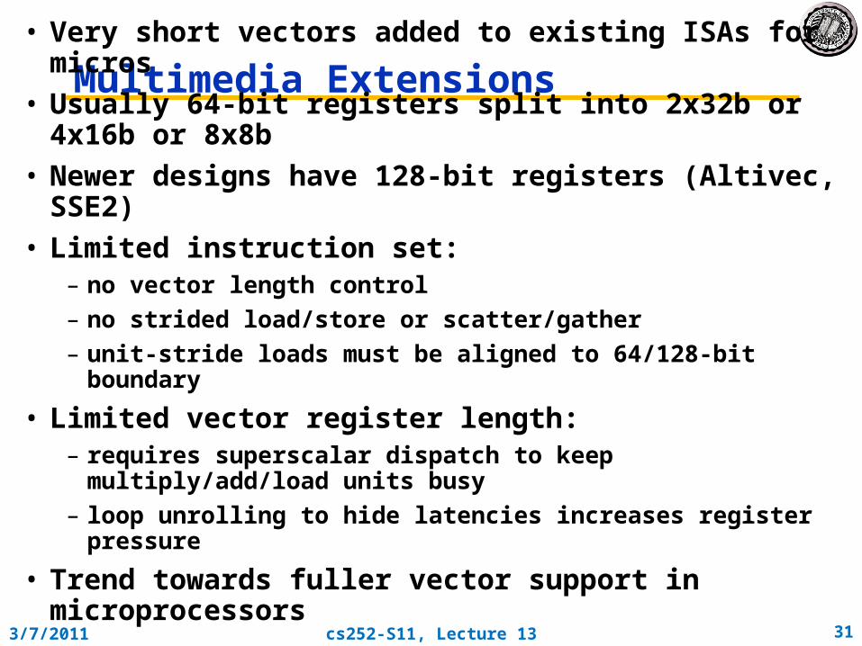
Multimedia Extensions• Very short vectors added to existing ISAs for micros
• Usually 64-bit registers split into 2x32b or 4x16b or 8x8b
• Newer designs have 128-bit registers (Altivec, SSE2)
• Limited instruction set:– no vector length control
– no strided load/store or scatter/gather
– unit-stride loads must be aligned to 64/128-bit boundary
• Limited vector register length:– requires superscalar dispatch to keep multiply/add/load units
busy
– loop unrolling to hide latencies increases register pressure
• Trend towards fuller vector support in microprocessors

3/7/2011 cs252-S11, Lecture 13 32
“Vector” for Multimedia?• Intel MMX: 57 additional 80x86 instructions (1st since
386)– similar to Intel 860, Mot. 88110, HP PA-71000LC, UltraSPARC
• 3 data types: 8 8-bit, 4 16-bit, 2 32-bit in 64bits– reuse 8 FP registers (FP and MMX cannot mix)
• short vector: load, add, store 8 8-bit operands
• Claim: overall speedup 1.5 to 2X for 2D/3D graphics, audio, video, speech, comm., ...
– use in drivers or added to library routines; no compiler
+

3/7/2011 cs252-S11, Lecture 13 33
MMX Instructions
• Move 32b, 64b
• Add, Subtract in parallel: 8 8b, 4 16b, 2 32b– opt. signed/unsigned saturate (set to max) if overflow
• Shifts (sll,srl, sra), And, And Not, Or, Xor in parallel: 8 8b, 4 16b, 2 32b
• Multiply, Multiply-Add in parallel: 4 16b
• Compare = , > in parallel: 8 8b, 4 16b, 2 32b– sets field to 0s (false) or 1s (true); removes branches
• Pack/Unpack– Convert 32b<–> 16b, 16b <–> 8b
– Pack saturates (set to max) if number is too large

3/7/2011 cs252-S11, Lecture 13 34
VLIW: Very Large Instruction Word
• Each “instruction” has explicit coding for multiple operations
– In IA-64, grouping called a “packet”
– In Transmeta, grouping called a “molecule” (with “atoms” as ops)
• Tradeoff instruction space for simple decoding– The long instruction word has room for many operations
– By definition, all the operations the compiler puts in the long instruction word are independent => execute in parallel
– E.g., 2 integer operations, 2 FP ops, 2 Memory refs, 1 branch» 16 to 24 bits per field => 7*16 or 112 bits to 7*24 or 168 bits wide
– Need compiling technique that schedules across several branches

3/7/2011 cs252-S11, Lecture 13 35
Recall: Unrolled Loop that Minimizes Stalls for Scalar
1 Loop: L.D F0,0(R1)2 L.D F6,-8(R1)3 L.D F10,-16(R1)4 L.D F14,-24(R1)5 ADD.D F4,F0,F26 ADD.D F8,F6,F27 ADD.D F12,F10,F28 ADD.D F16,F14,F29 S.D 0(R1),F410 S.D -8(R1),F811 S.D -16(R1),F1212 DSUBUI R1,R1,#3213 BNEZ R1,LOOP14 S.D 8(R1),F16 ; 8-32 = -24
14 clock cycles, or 3.5 per iteration
L.D to ADD.D: 1 CycleADD.D to S.D: 2 Cycles

3/7/2011 cs252-S11, Lecture 13 36
Loop Unrolling in VLIWMemory Memory FP FP Int. op/ Clockreference 1 reference 2 operation 1 op. 2 branch
L.D F0,0(R1) L.D F6,-8(R1) 1
L.D F10,-16(R1) L.D F14,-24(R1) 2
L.D F18,-32(R1) L.D F22,-40(R1) ADD.D F4,F0,F2 ADD.D F8,F6,F2 3
L.D F26,-48(R1) ADD.D F12,F10,F2 ADD.D F16,F14,F2 4
ADD.D F20,F18,F2 ADD.D F24,F22,F2 5
S.D 0(R1),F4 S.D -8(R1),F8 ADD.D F28,F26,F2 6
S.D -16(R1),F12 S.D -24(R1),F16 7
S.D -32(R1),F20 S.D -40(R1),F24 DSUBUI R1,R1,#48 8
S.D -0(R1),F28 BNEZ R1,LOOP 9
Unrolled 7 times to avoid delays
7 results in 9 clocks, or 1.3 clocks per iteration (1.8X)
Average: 2.5 ops per clock, 50% efficiency
Note: Need more registers in VLIW (15 vs. 6 in SS)

3/7/2011 cs252-S11, Lecture 13 37
Paper Discussion: VLIW and the ELI-512Joshua Fisher
• Trace Scheduling:– Find common paths through code (“Traces”)– Compact them– Build fixup code for trace exits (the “split” boxes)– Must not overwrite live variables use extra variables to store results
• N+1 way jumps– Used to handle exit conditions from traces
• Software prediction of memory bank usage– Use it to avoid bank conflicts/deal with limited routing

3/7/2011 cs252-S11, Lecture 13 38
Problems with 1st Generation VLIW• Increase in code size
– generating enough operations in a straight-line code fragment requires ambitiously unrolling loops
– whenever VLIW instructions are not full, unused functional units translate to wasted bits in instruction encoding
• Operated in lock-step; no hazard detection HW– a stall in any functional unit pipeline caused entire
processor to stall, since all functional units must be kept synchronized
– Compiler might prediction function units, but caches hard to predict
• Binary code compatibility– Pure VLIW => different numbers of functional units and
unit latencies require different versions of the code
3/7/2011 cs252-S11, Lecture 13 39
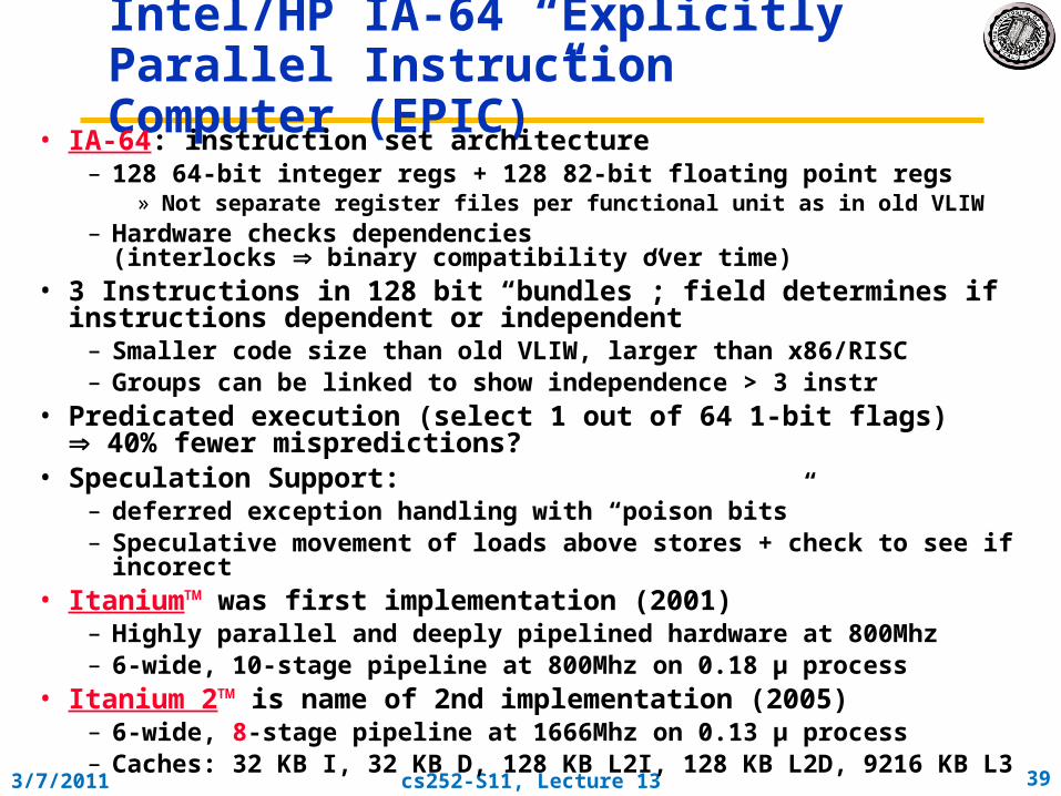
Intel/HP IA-64 “Explicitly Parallel Instruction Computer (EPIC)”
• IA-64: instruction set architecture– 128 64-bit integer regs + 128 82-bit floating point regs
» Not separate register files per functional unit as in old VLIW– Hardware checks dependencies
(interlocks binary compatibility over time)• 3 Instructions in 128 bit “bundles”; field determines if instructions
dependent or independent– Smaller code size than old VLIW, larger than x86/RISC– Groups can be linked to show independence > 3 instr
• Predicated execution (select 1 out of 64 1-bit flags) 40% fewer mispredictions?
• Speculation Support: – deferred exception handling with “poison bits”– Speculative movement of loads above stores + check to see if incorect
• Itanium™ was first implementation (2001)– Highly parallel and deeply pipelined hardware at 800Mhz– 6-wide, 10-stage pipeline at 800Mhz on 0.18 µ process
• Itanium 2™ is name of 2nd implementation (2005)– 6-wide, 8-stage pipeline at 1666Mhz on 0.13 µ process– Caches: 32 KB I, 32 KB D, 128 KB L2I, 128 KB L2D, 9216 KB L3

3/7/2011 cs252-S11, Lecture 13 40
Branch Hints
Memory Hints
InstructionCache
& BranchPredictors
FetchFetch Memory Memory SubsystemSubsystem
Three levels of cache:L1, L2, L3
Register Stack & Rotation
Explicit Parallelism
128 GR &128 FR,RegisterRemap
&Stack Engine
Register Register HandlingHandling
Fast, S
imp
le 6-Issue
IssueIssue ControlControl
Micro-architecture Features in hardwareMicro-architecture Features in hardware: :
Itanium™ EPIC Design Maximizes SW-HW Synergy
(Copyright: Intel at Hotchips ’00)Architecture Features programmed by compiler::
PredicationData & ControlSpeculation
Byp
asse
s & D
ep
end
encie
s
Parallel ResourcesParallel Resources
4 Integer + 4 MMX Units
2 FMACs (4 for SSE)
2 LD/ST units
32 entry ALAT
Speculation Deferral Management

3/7/2011 cs252-S11, Lecture 13 41
10 Stage In-Order Core Pipeline(Copyright: Intel at Hotchips ’00)
Front EndFront End• Pre-fetch/Fetch of up Pre-fetch/Fetch of up to 6 instructions/cycleto 6 instructions/cycle
• Hierarchy of branch Hierarchy of branch predictorspredictors
• Decoupling bufferDecoupling buffer
Instruction DeliveryInstruction Delivery• Dispersal of up to 6 Dispersal of up to 6 instructions on 9 portsinstructions on 9 ports
• Reg. remappingReg. remapping• Reg. stack engineReg. stack engine
Operand DeliveryOperand Delivery• Reg read + Bypasses Reg read + Bypasses • Register scoreboardRegister scoreboard• Predicated Predicated
dependencies dependencies
ExecutionExecution• 4 single cycle ALUs, 2 ld/str4 single cycle ALUs, 2 ld/str• Advanced load control Advanced load control • Predicate delivery & branchPredicate delivery & branch• Nat/Exception/Nat/Exception///RetirementRetirement
IPG FET ROT EXP REN REG EXE DET WRBWLD
REGISTER READWORD-LINE DECODERENAMEEXPAND
INST POINTER GENERATION
FETCH ROTATE EXCEPTIONDETECT
EXECUTE WRITE-BACK

3/7/2011 cs252-S11, Lecture 13 42
What is Parallel Architecture?• A parallel computer is a collection of processing
elements that cooperate to solve large problems– Most important new element: It is all about communication!
• What does the programmer (or OS or Compiler writer) think about?
– Models of computation: » PRAM? BSP? Sequential Consistency?
– Resource Allocation:» how powerful are the elements?» how much memory?
• What mechanisms must be in hardware vs software– What does a single processor look like?
» High performance general purpose processor» SIMD processor/Vector Processor
– Data access, Communication and Synchronization» how do the elements cooperate and communicate?» how are data transmitted between processors?» what are the abstractions and primitives for cooperation?

3/7/2011 cs252-S11, Lecture 13 43
Flynn’s Classification (1966)Broad classification of parallel computing systems
• SISD: Single Instruction, Single Data– conventional uniprocessor
• SIMD: Single Instruction, Multiple Data– one instruction stream, multiple data paths
– distributed memory SIMD (MPP, DAP, CM-1&2, Maspar)
– shared memory SIMD (STARAN, vector computers)
• MIMD: Multiple Instruction, Multiple Data– message passing machines (Transputers, nCube, CM-5)
– non-cache-coherent shared memory machines (BBN Butterfly, T3D)
– cache-coherent shared memory machines (Sequent, Sun Starfire, SGI Origin)
• MISD: Multiple Instruction, Single Data– Not a practical configuration

3/7/2011 cs252-S11, Lecture 13 44
Examples of MIMD Machines• Symmetric Multiprocessor
– Multiple processors in box with shared memory communication
– Current MultiCore chips like this– Every processor runs copy of OS
• Non-uniform shared-memory with separate I/O through host
– Multiple processors » Each with local memory» general scalable network
– Extremely light “OS” on node provides simple services
» Scheduling/synchronization– Network-accessible host for I/O
• Cluster– Many independent machine connected
with general network – Communication through messages
P P P P
Bus
Memory
P/M P/M P/M P/M
P/M P/M P/M P/M
P/M P/M P/M P/M
P/M P/M P/M P/M
Host
Network

3/7/2011 cs252-S11, Lecture 13 45
Categories of Thread ExecutionTi
me
(pro
cess
or
cycle
)Superscalar Fine-Grained Coarse-Grained Multiprocessing
SimultaneousMultithreading
Thread 1
Thread 2Thread 3Thread 4
Thread 5Idle slot
3/7/2011 cs252-S11, Lecture 13 46
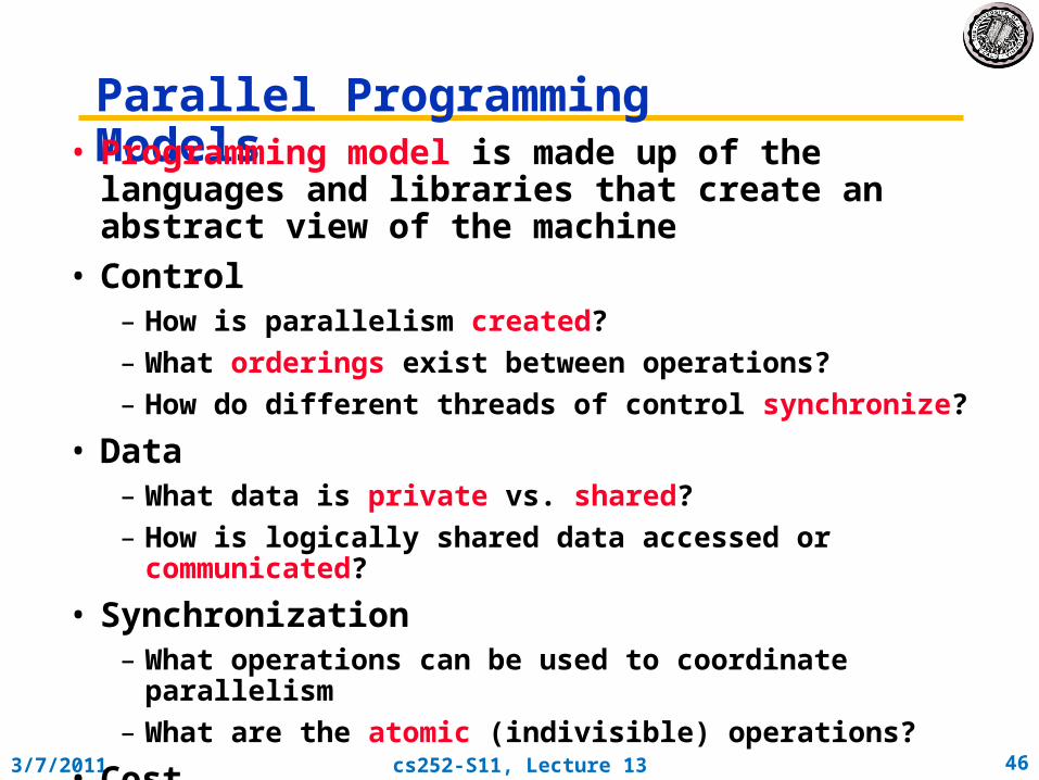
Parallel Programming Models• Programming model is made up of the languages and libraries that create an abstract view of the machine
• Control– How is parallelism created?
– What orderings exist between operations?
– How do different threads of control synchronize?
• Data– What data is private vs. shared?
– How is logically shared data accessed or communicated?
• Synchronization– What operations can be used to coordinate parallelism
– What are the atomic (indivisible) operations?
• Cost– How do we account for the cost of each of the above?

3/7/2011 cs252-S11, Lecture 13 47
Simple Programming Example
• Consider applying a function f to the elements of an array A and then computing its sum:
• Questions:– Where does A live? All in single memory?
Partitioned?
– What work will be done by each processors?
– They need to coordinate to get a single result, how?
1
0
])[(n
i
iAf
A:
fA:f
sum
A = array of all datafA = f(A)s = sum(fA)
s:
3/7/2011 cs252-S11, Lecture 13 48
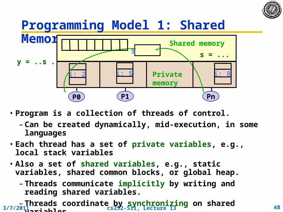
Programming Model 1: Shared Memory
• Program is a collection of threads of control.
– Can be created dynamically, mid-execution, in some languages
• Each thread has a set of private variables, e.g., local stack variables
• Also a set of shared variables, e.g., static variables, shared common blocks, or global heap.
– Threads communicate implicitly by writing and reading shared variables.
– Threads coordinate by synchronizing on shared variables
PnP1P0
s s = ...y = ..s ...
Shared memory
i: 2 i: 5 Private memory
i: 8
3/7/2011 cs252-S11, Lecture 13 49
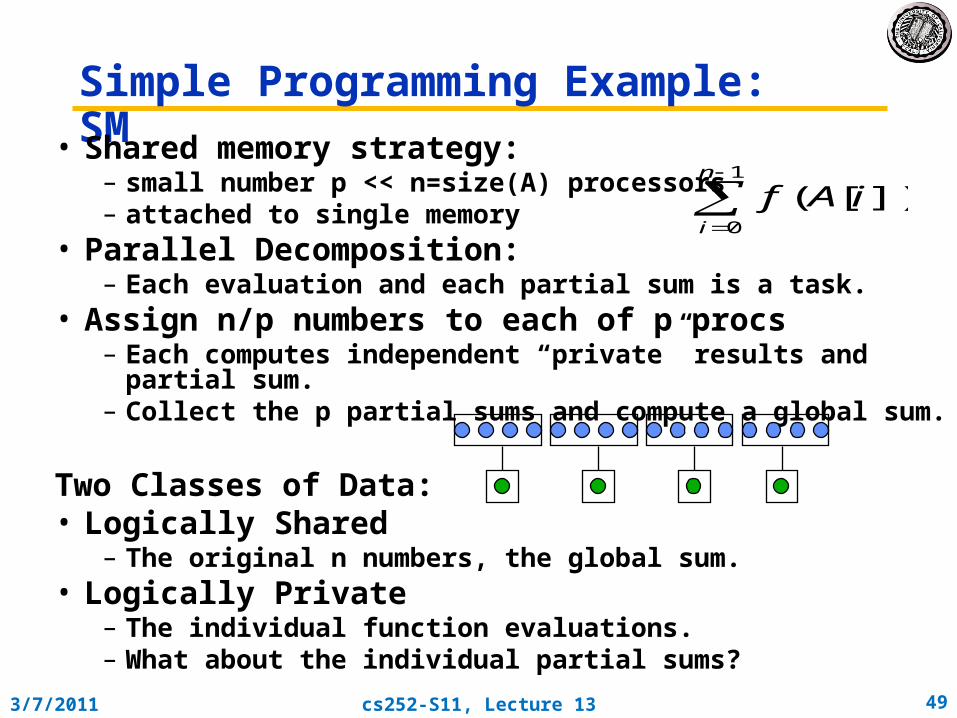
Simple Programming Example: SM• Shared memory strategy:
– small number p << n=size(A) processors – attached to single memory
• Parallel Decomposition: – Each evaluation and each partial sum is a task.
• Assign n/p numbers to each of p procs– Each computes independent “private” results and partial sum.– Collect the p partial sums and compute a global sum.
Two Classes of Data: • Logically Shared
– The original n numbers, the global sum.• Logically Private
– The individual function evaluations.– What about the individual partial sums?
1
0
])[(n
i
iAf

3/7/2011 cs252-S11, Lecture 13 50
Shared Memory “Code” for sum
Thread 1
for i = 0, n/2-1 s = s + f(A[i])
Thread 2
for i = n/2, n-1 s = s + f(A[i])
static int s = 0;
• Problem is a race condition on variable s in the program• A race condition or data race occurs when:
- two processors (or two threads) access the same variable, and at least one does a write.
- The accesses are concurrent (not synchronized) so they could happen simultaneously
3/7/2011 cs252-S11, Lecture 13 51
A Closer Look
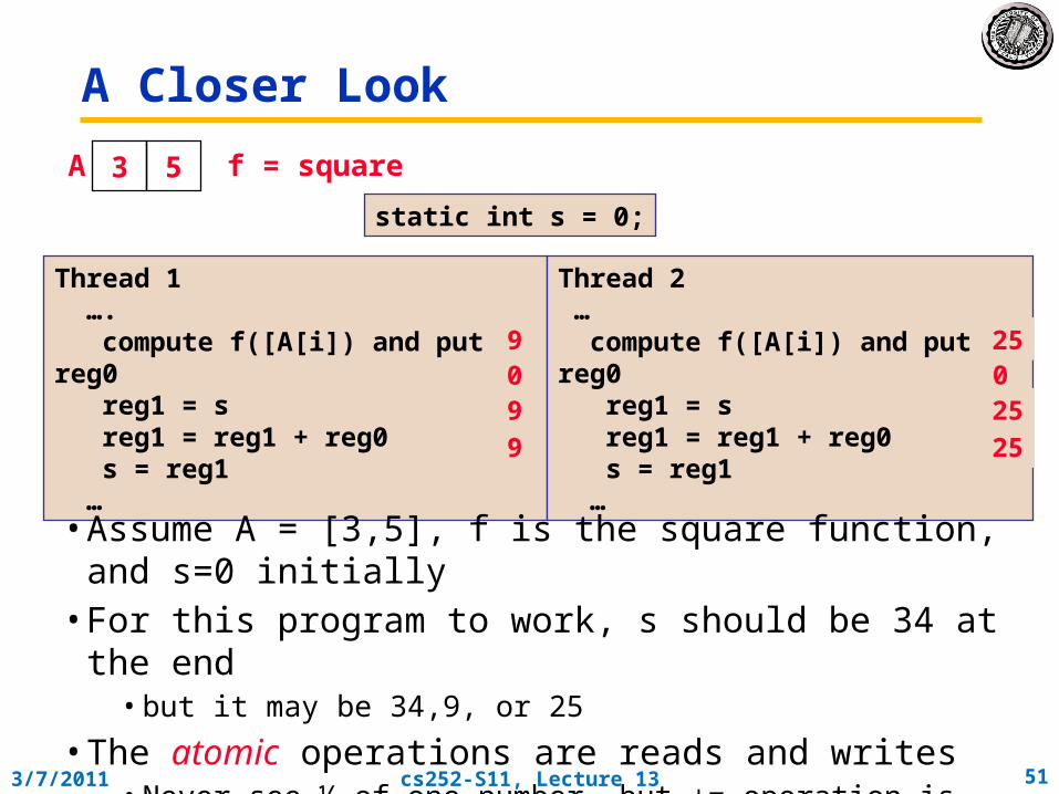
Thread 1 …. compute f([A[i]) and put in reg0 reg1 = s reg1 = reg1 + reg0 s = reg1 …
Thread 2 … compute f([A[i]) and put in reg0 reg1 = s reg1 = reg1 + reg0 s = reg1 …
static int s = 0;
• Assume A = [3,5], f is the square function, and s=0 initially• For this program to work, s should be 34 at the end
• but it may be 34,9, or 25
• The atomic operations are reads and writes• Never see ½ of one number, but += operation is not atomic• All computations happen in (private) registers
9 250 09 25
259
3 5A f = square

3/7/2011 cs252-S11, Lecture 13 52
Improved Code for Sum
Thread 1
local_s1= 0 for i = 0, n/2-1 local_s1 = local_s1 + f(A[i]) s = s + local_s1
Thread 2
local_s2 = 0 for i = n/2, n-1 local_s2= local_s2 + f(A[i]) s = s +local_s2
static int s = 0;
• Since addition is associative, it’s OK to rearrange order• Most computation is on private variables
- Sharing frequency is also reduced, which might improve speed - But there is still a race condition on the update of shared s
- The race condition can be fixed by adding locks (only one thread can hold a lock at a time; others wait for it)
static lock lk;
lock(lk);
unlock(lk);
lock(lk);
unlock(lk);

3/7/2011 cs252-S11, Lecture 13 53
What about Synchronization?• All shared-memory programs need synchronization• Barrier – global (/coordinated) synchronization
– simple use of barriers -- all threads hit the same one work_on_my_subgrid(); barrier; read_neighboring_values(); barrier;• Mutexes – mutual exclusion locks
– threads are mostly independent and must access common data lock *l = alloc_and_init(); /* shared */ lock(l); access data unlock(l);• Need atomic operations bigger than loads/stores
– Actually – Dijkstra’s algorithm can get by with only loads/stores, but this is quite complex (and doesn’t work under all circumstances)
– Example: atomic swap, test-and-test-and-set• Another Option: Transactional memory
– Hardware equivalent of optimistic concurrency– Some think that this is the answer to all parallel programming

3/7/2011 cs252-S11, Lecture 13 54
Programming Model 2: Message Passing
• Program consists of a collection of named processes.– Usually fixed at program startup time
– Thread of control plus local address space -- NO shared data.
– Logically shared data is partitioned over local processes.
• Processes communicate by explicit send/receive pairs– Coordination is implicit in every communication event.
– MPI (Message Passing Interface) is the most commonly used SW
PnP1P0
y = ..s ...
s: 12
i: 2
Private memory
s: 14
i: 3
s: 11
i: 1
send P1,s
Network
receive Pn,s

3/7/2011 cs252-S11, Lecture 13 55
Compute A[1]+A[2] on each processor° First possible solution – what could go wrong?
Processor 1 xlocal = A[1] send xlocal, proc2 receive xremote, proc2 s = xlocal + xremote
Processor 2 xloadl = A[2] receive xremote, proc1 send xlocal, proc1 s = xlocal + xremote
° Second possible solution
Processor 1 xlocal = A[1] send xlocal, proc2 receive xremote, proc2 s = xlocal + xremote
Processor 2 xlocal = A[2] send xlocal, proc1 receive xremote, proc1 s = xlocal + xremote
° If send/receive acts like the telephone system? The post office?
° What if there are more than 2 processors?

3/7/2011 cs252-S11, Lecture 13 56
MPI – the de facto standard• MPI has become the de facto standard for parallel
computing using message passing• Example:
for(i=1;i<numprocs;i++) { sprintf(buff, "Hello %d! ", i); MPI_Send(buff, BUFSIZE, MPI_CHAR, i, TAG,
MPI_COMM_WORLD); } for(i=1;i<numprocs;i++) {
MPI_Recv(buff, BUFSIZE, MPI_CHAR, i, TAG, MPI_COMM_WORLD, &stat);
printf("%d: %s\n", myid, buff); }
• Pros and Cons of standards– MPI created finally a standard for applications development in
the HPC community portability– The MPI standard is a least common denominator building on
mid-80s technology, so may discourage innovation

3/7/2011 cs252-S11, Lecture 13 57
Which is better? SM or MP?• Which is better, Shared Memory or Message Passing?
– Depends on the program!– Both are “communication Turing complete”
» i.e. can build Shared Memory with Message Passing and vice-versa
• Advantages of Shared Memory:– Implicit communication (loads/stores)– Low overhead when cached
• Disadvantages of Shared Memory:– Complex to build in way that scales well– Requires synchronization operations– Hard to control data placement within caching system
• Advantages of Message Passing– Explicit Communication (sending/receiving of messages)– Easier to control data placement (no automatic caching)
• Disadvantages of Message Passing– Message passing overhead can be quite high– More complex to program– Introduces question of reception technique (interrupts/polling)
3/7/2011 cs252-S11, Lecture 13 58
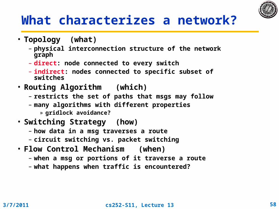
What characterizes a network?
• Topology (what)– physical interconnection structure of the network graph– direct: node connected to every switch– indirect: nodes connected to specific subset of switches
• Routing Algorithm (which)– restricts the set of paths that msgs may follow– many algorithms with different properties
» gridlock avoidance?
• Switching Strategy (how)– how data in a msg traverses a route– circuit switching vs. packet switching
• Flow Control Mechanism (when)– when a msg or portions of it traverse a route– what happens when traffic is encountered?

3/7/2011 cs252-S11, Lecture 13 59
Example: Multidimensional Meshes and Tori
• n-dimensional array– N = kd-1 X ...X kO nodes
– described by n-vector of coordinates (in-1, ..., iO)
• n-dimensional k-ary mesh: N = kn
– k = nN
– described by n-vector of radix k coordinate
• n-dimensional k-ary torus (or k-ary n-cube)?
2D Grid 3D Cube2D Torus

3/7/2011 cs252-S11, Lecture 13 60
Links and Channels
• transmitter converts stream of digital symbols into signal that is driven down the link
• receiver converts it back– tran/rcv share physical protocol
• trans + link + rcv form Channel for digital info flow between switches
• link-level protocol segments stream of symbols into larger units: packets or messages (framing)
• node-level protocol embeds commands for dest communication assist within packet
Transmitter
...ABC123 =>
Receiver
...QR67 =>

3/7/2011 cs252-S11, Lecture 13 61
Clock Synchronization?• Receiver must be synchronized to transmitter
– To know when to latch data
• Fully Synchronous– Same clock and phase: Isochronous– Same clock, different phase: Mesochronous
» High-speed serial links work this way» Use of encoding (8B/10B) to ensure sufficient high-frequency
component for clock recovery
• Fully Asynchronous– No clock: Request/Ack signals– Different clock: Need some sort of clock recovery?
Data
Req
Ack
Transmitter Asserts Data
t0 t1 t2 t3 t4 t5

3/7/2011 cs252-S11, Lecture 13 62
Conclusion• Vector is alternative model for exploiting ILP
– If code is vectorizable, then simpler hardware, more energy efficient, and better real-time model than Out-of-order machines
– Design issues include number of lanes, number of functional units, number of vector registers, length of vector registers, exception handling, conditional operations
• Will multimedia popularity revive vector architectures?• Multiprocessing
– Multiple processors connect together– It is all about communication!
• Programming Models:– Shared Memory– Message Passing
• Networking and Communication Interfaces– Fundamental aspect of multiprocessing
Recommended