Credibility, Pre-Production and Inviting Competition in a Network Market
Amir Etzionya and
Avi Weissa,b,*
aDepartment of Economics, Bar-Ilan University, 52900 Ramat-Gan, Israel bIZA
October 2001
Credibility, Pre-Production and Inviting Competition in a Network Market
Abstract
In this paper we considered a new solution to the credibility problem present in network industries. This problem arises because the value of a network good to its owner depends positively on the number of consumers who buy the good. Because of this property, it is in the interest of the producer to try to convince consumers that the market will be large, even if he knows it is untrue. Consumers, in turn, will disregard producer claims, and will, instead, try to reason out what size the market will attain. As a result, a lower than optimal quantity, both for consumers and producers, will be produced, i.e., the resulting equilibrium is Pareto inefficient. Katz and Shapiro (1985) and Economides (1996) suggest a solution to this problem in which the firm invites competitors to share their technology and enter the market, thus voluntarily giving up their monopoly position. We suggest an alternative remedy of pre-producing the good. This has the effect of changing the firm’s cost structure in a manner that causes consumers to believe that the amount they will optimally sell (and hence the market size) will increase, again leading to higher profitability. The two strategies are compared, and we show the conditions under which each is preferable. We then consider combinations of these two strategies in two different manners. In the first the leader produces and then invites competitors who then also pre-produce, and in the second the leader pre-produces but the fringe firms do not; rather, they produce in the same period in which they sell. Surprisingly we found that the latter dominated the former, which led us to a better understanding about how and why each strategy works. In short, inviting competitors creates a positive externality that benefits all firms, while pre-producing helps only the firm doing the pre-producing and harms all other firms. Thus, the leader invites competitors so he can benefit from the positive externality, but he is better off if the competitors do not pre-produce. Keywords: Network market, pre-production, inviting competition, network externalities. JEL codes: D21, D43

I. Introduction
One of the main characteristics of network goods is that the value of the product
to each consumer increases with the number of consumers who own the product.
Because of this property, the willingness of any particular consumer to buy the
product will depend not only on the price of the good, but also on the size of the
market. When a new product is introduced to a market, however, consumers do not
know what size the market will attain, and so must base their decisions on beliefs.
One source from which consumers can obtain information is from the declarations
made by the producer about his production intentions. However, the producer has a
clear incentive to overstate the expected market size in order to be able to increase the
price, so these declarations may not be credible. Thus, the consumer may discount this
information, and try instead to reason what the firm will do optimally given consumer
behavior. The result of this is that a Pareto inferior equilibrium will be attained, while
if the producer could somehow convince the consumers that his intentions are sincere,
and, in fact, he carried through on those intentions, all parties would be made strictly
better off.1
Katz and Shapiro (1985) and Economides (1996) address this issue. They suggest
that one way to overcome, at least partially, this confidence problem, is for the firm to
voluntarily relinquish its monopoly position by inviting competitors into the market.
The result of the increased competition is to increase consumer expectations about the
size of the market because of the effect competition usually has on production.
Consequently, the quantity the firm can sell increases, and under certain conditions
the firm’s profits increase.
In this paper we suggest an alternative strategy. The main tenet is that the firm
may be able to take steps that will change its cost structure in a way that convinces
consumers that a larger quantity will be supplied. In particular, if the firm can lower
marginal costs the amount consumers believe will be produced increases, and, in turn,
so does the quantity actually bought. While there may be a number of ways to lower
marginal costs, the one we investigate is pre-production by the firm. This has the
1 Another source of uncertainty is with respect to the behavior of other consumers. Specifically, consumers must not only be convinced about producer behavior, they must be convinced that other consumers will buy the product. When each consumer’s decision to buy depends on the purchase of the others, this requires common knowledge of beliefs for purchase to actually occur. Etziony and Weiss (2001) address this issue in an experimental setting.

2
effect of lowering marginal costs to zero, and, in fact, turning the variable costs into
fixed costs. This strategy was suggested by Spence (1977), Dixit (1980), Ware (1983)
and Allen (1993), among others, as a way of convincing potential competitors about
actions. We show how this strategy can also be used to convince consumers about
actions, which will consequently benefit the firm. Interestingly, using this tool in the
manner we suggest leads to an increase in both producer and consumer welfare, which
also distinguishes our results from those in previous studies. After developing the
model, we compare between this strategy and that of inviting competition. We also
combine the strategies and show the optimal combination under different cost and
demand conditions.
We begin by demonstrating the credibility problem faced by producers in a
network market in Section II. Section III contains the solution of pre-production, and
in Section IV we compare this solution with that of inviting competitors as developed
in Economides (1996). In Section V the two strategies are combined under two
possible scenarios. In the first, all firms produce before the selling stage, although the
inviting firm produces before the other firms, and is thus a Stackelberg leader in the
market. In the second, only the inviting firm pre-produces. All strategies are then
compared in Section VI, and insight into the way each strategy works is derived from
the comparison. A short summary and discussion are presented in Section VII.
II. The Credibility Problem in Network Markets
A credibility problem in a network market is said to exist in a situation in which a
producer of a good has an incentive to misstate his intentions in order to affect the
behavior of consumers or of other producers. An example of the latter is what has
been termed “vaporware” – an announcement by a firm about the expected release
date of a new product or about the capabilities of a new product, even when these
statements are false. The purpose of these announcements is to depress competition
(see Levy, 1996, Cass and Hylton, 1999, Dranove and Gandal, 2000, and Bayus, 2001
for analyses).
With respect to misleading consumers, the essence of network goods makes
exaggerated statements about the size of the market particularly valuable to the
producer if he can get consumers to believe him. This is because of the effect
purchase by others has on the value each consumer attributes to the good. Consumers,
recognizing this incentive, will discount any statements made by the producer. The

3
result of this is that consumers will not believe some statements of intent, which, if
carried out, would be beneficial to all parties. This will be the case when it is not in
the producer’s interest to carry out these actions ex-post, even if it is in his interest ex-
ante.
Most previous studies of this problem considered a multi-period setting with a
basic durable good and complementary goods. Consider, for instance, a consumer
considering buying a home video-game system. The reason a consumer purchases
such a product is because of the games he will be able to play, and not because of the
hardware. If there is only a small stock of existing games, and he believes there will
be few games made for the machine in the future, he may be reluctant to make the
purchase. In addition, if he believes the cost of games will be increased significantly,
he may not purchase the system. The producer could attempt to convince consumers
that games will be made available and that prices will be kept low, but the consumer
may believe that the producer will be more concerned with creating the next
generation of machines than with the creation of new games for machines that were
already purchased, and that there will be nothing compelling the producer not to
increase prices once the machines have been bought. The inability of producers to
credibly commit to actions in future periods is particularly acute in high-tech
industries because of the high rate of technological progress. In the case just
discussed, the creation of a large stock of games in the first period, or the presence of
competitors willing to make new games can help convince consumers that this will
not be a problem.
Farrel and Gallini (1988) discuss a situation in which before purchasing a good,
consumers must bear a setup cost in order to benefit from the product. This cost could
be a training cost or the purchase of hardware necessary to use the software in which
he is really interested (as in the example in the last paragraph). This leads to an ex-
post opportunism problem, because the producer can use the fact that the cost has
been sunk, and can then increase the price of the good. Klemperer (1987), Farrel and
Shapiro (1988, 1989) and Beggs and Klemperer (1992) analyze this possibility in a
case in which the firm determines the setup cost, and consumers, after paying this
setup cost, must bear a switching cost to move to a competing product (see
Klemperer, 1995, for a survey). In Williamson’s (1975) terms this industry suffers
from a “hold-up” problem – a combination of ex-post small numbers (once the sunk
cost is made only the producer can supply the product) and opportunism, a

4
combination that has also been denoted a lock-in problem (e.g., Varian, 1999). This
type of problem can, of course, cause the consumer to not buy the product.
All these studies considered indirect network externalities, where the consumption
of others is important because of the effect the size of the market has on the
availability of complementary goods. Katz and Shapiro (1985) were the first to
discuss the credibility problem in a market with direct network externalities, where
the base good itself becomes more valuable as the market size increases (as in the
case of telephones and fax machines). In their model, consumers’ beliefs about the
market size are determined prior to the producer deciding how much to produce and
sell. Once determined, these beliefs can no longer be changed. The producer takes
these beliefs into account in deciding how much to produce. This problem is
reexamined and expanded in Economides (1993, 1996) in a setting in which consumer
belief-formation and production occur concurrently.
A short exposition of the problem, based on the Economides (1996) model will
help bring the salient features of the credibility problem in a one period model into
focus. We start with a differentiable, separable inverse demand function for the
network good:
)()(),( SfQPSQP +≡ ,
where Q is the actual quantity of the good sold and S the amount consumers expect to
be sold. The first part of the inverse demand curve shows the direct effect of the
quantity demanded on price, with QQQP
QSQP
∀<∂
∂=
∂∂ 0 )(),( . The second part is the
network effect, with SQS
f(S)S
SQP , 0),(∀≥
∂∂
=∂
∂ . To make the presentation simple, we
assume linear functions, so that (1) becomes:
eSQaSQP +−=),( , e<1.
The producer’s technology is CRS, with constant marginal costs equal to c. If the
producer were accounted full credibility, in that any quantity he announced would be
believed and produced, then he would face the demand curve:
QeaQQP )1(),( −−=
and the optimal quantity would be given by:
(1) )1(200 e
caSQ−−
== .

5
Assume, then, that the producer declares that he will produce 0Q units and that
consumers believe him, so that 00 QS = . In this case, when deciding how much to
actually produce the firm would maximize:
00 ),( eSQaSQP +−= ,
and the quantity produced would be
(2) 2
)( 00
* eScaSQ +−= .
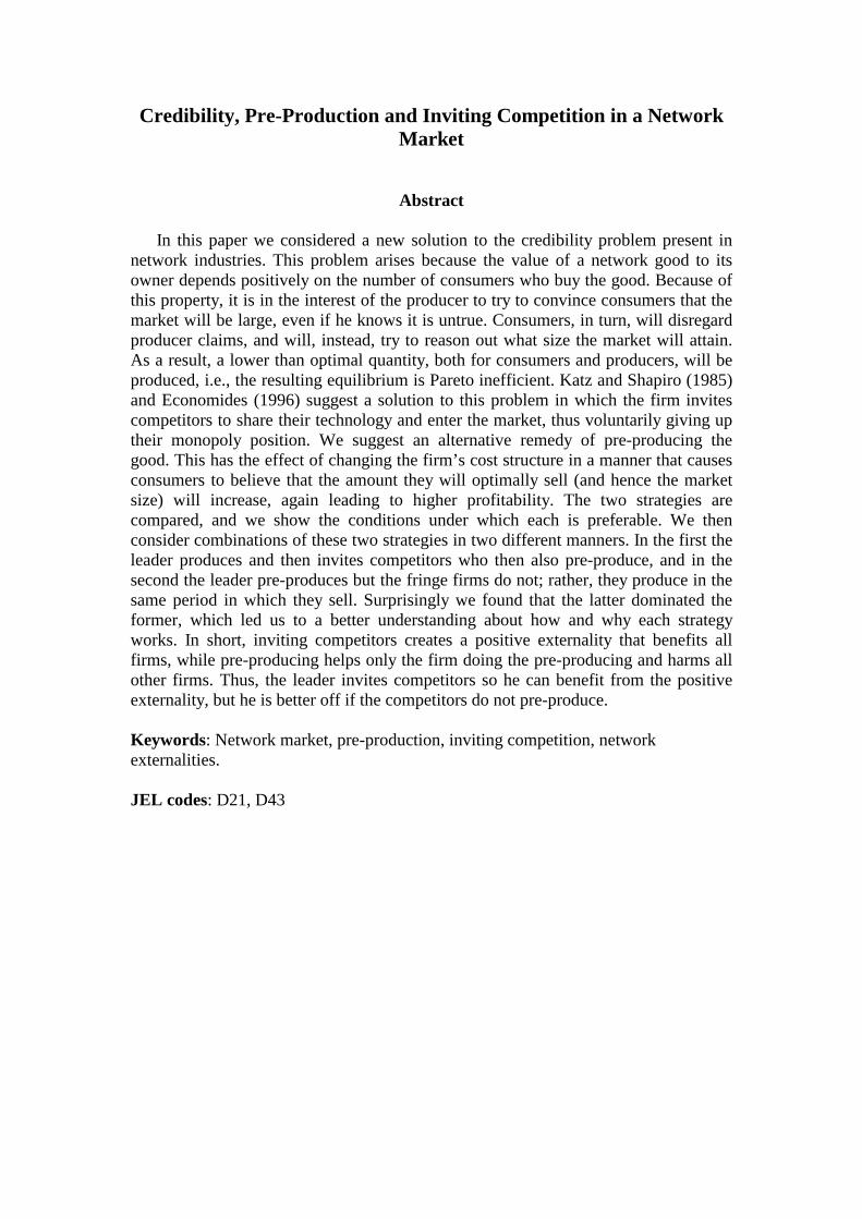
By substituting (1) into (2) and comparing, it is easy to see that 00* )( QSQ < . Thus,
the firm overstates the amount it will produce, and the credibility problem is born.
The problem is demonstrated in Figure 1. The fulfilled expectations demand curve is
more elastic than the demand curve actually facing the producer. This gives him an
incentive to produce less than consumers expect.
Consumers, anticipating this result, do not believe that the producer will produce
the amount defined in (1). There exists, however, an equilibrium at which the amount
consumers believe will be produced equals the amount the firm optimally produces.
To find this equilibrium graphically, we construct two reaction functions, that of the
informed consumer who knows how much will be produced, i.e., QSRC =: , and that
of the producer as per (2): SecaQRF 22: +
−= . Equilibrium is attained when these
are equal:
ecaQE −
−=
2.
This equilibrium is demonstrated in Figure 2. This equilibrium is attained
mathematically by maximizing profits for a fixed level of S, and then setting S=Q.
Note that in this instance the firm suffers from a total lack of credibility, and is unable
to affect consumer beliefs at all. Clearly both consumers and producers would be
better off at 0Q than at EQ , but because of the credibility problem an inferior
equilibrium is attained.
III. Pre-Production
To allow for comparison with the strategy of inviting competition developed in
Katz and Shapiro (1985) and Economides (1996), we use the same functional forms
used in the Economides model. Consider first a monopolist that is unable to either

6
pre-produce or invite competition. The monopolist produces a new network good, and
faces the inverse demand curve )(),( SfQaSQP +−= , where Q is total industry
purchases and S is the amount consumers believe will be purchased, 0>′f . The
production technology is assumed to be CRS, so marginal costs are constant and equal
to c. The firm’s optimization problem is:
cQf(S)) QQ(aQQ
−+−=Π MaxMax .
Note that because of the credibility problem, S is a parameter in this objective
function. The quantity and profits of the producer in equilibrium, denoted by nsQ and nsΠ (the superscripts stand for “no strategy”), respectively, are:
(3) 2
2;
2
−+=Π
−+=
c)f(Qac)f(QaQns
nsns
ns ,
with the condition that 1)( <′ nsQf for this to be a maximum, since if 1)( >′ nsQf it
is always worthwhile to increase production.
Consider now pre-production (pp). The game now consists of two periods. In the
first period (denoted period 0) the firm has the option to produce any quantity of the
product at marginal cost c. In period 1 the firm can sell some or all of what was
produced, and increase production with the same marginal cost. For simplicity we
assume that there is no storage cost.2 Since the firm is, in essence, limiting its options
by producing a large quantity of the good before marketing, it would seem to be
harmful to the firm because it reduces the firm’s strategy space. However, as in
Spence (1977), Dixit (1980), Ware (1983) and Allen (1993), we show that this
actually leads to increased profits. As mentioned above, the difference in our setting
from the setting in those earlier studies is that here the source of the benefit is from
the effect on consumers, while in the earlier studies it is because of the effect on
potential competitors. In addition, one of the results of our model is that both producer
and consumer welfare increases when pre-production occurs, which also distinguishes
our results from those in previous studies.
As a result of pre-production, the firm’s marginal cost structure in the selling
period is
2 We make this assumption because of the complexity of the solution. Simplification of the model might allow for explicitly including a storage cost, and one of the central questions would be how this cost affects the incentive to, and profitability of, pre-producing.

7
(4)
>=≤=
pppp
pppp
QQc formcQQ formc
0
0
0
where ppQ0 is the amount pre-produced and ppQ is the amount actually sold. As will
be shown shortly, the quantity produced optimally in the pre-production stage will be
greater than that when the firm cannot pre-produce. Thus, there is never any reason
for the firm to produce also in the selling period, and the bottom part of (4) becomes
irrelevant. To simplify the exposition, we therefore assume that the firm cannot
produce in the selling period.
We will solve the firm’s objective function in stages. Assume, first, that the firm
produced ppQ0 units in period 0, and let us assume for now that this quantity is
sufficient to supply the firm with all the units it will desire to sell in period 1. The
firm has thus borne a cost equal to ppcQ0 . Denote by ppQ the amount the firm
chooses to sell in the selling period under these circumstances. The firm’s objective
function given consumer expectations is given by: pppppp
QcQQf(S)) Q(aMax
pp 0−+−=Π .
Solving this yields an optimal quantity sold of
2f(S)aQ pp +
= .
Consumers, on their part, know that if the firm has produced ppQ units it will sell
them all, but the firm will never sell more than ppQ units even if it has already
produced those units. Thus, ppQS ≤ . In the case of equality we can better define ppQ by:
( )2
pppp Qfa
Q+
=
Consider now what happens if the firm produces less than ppQ units, i.e.,
pppp QQ <0 . In this case, consumers will certainly believe that the firm will sell its
entire pre-produced quantity, since it would want to sell ppQ units in period 1, were
that quantity available. Thus, consumer expectations can be summed up as follows:
≤
= otherwise
if 00pp
pppppp
QQQQ
S

8
These expectations are demonstrated in Figure 3.
Given these expectations, we now return to the firm’s strategy in period 0. Since
consumers will never believe that a quantity greater than ppQ will be sold, even if it
has been produced, the firm will never produce more than ppQ units. Below that
quantity, consumers believe that the quantity produced will all be sold. Thus,
dropping the subscript, the firm’s objective function is:
(5) [ ]
0s.t.
)(Maxpppp
pppppp
QcQfQa
≤≤
−+−
Which yields the following solution:
(6) [ ]
+
+≤<+′
′−
−+
<+
=
otherwise2
2 if2
if0
)Qf(a
)f(Qac)f(Qa)(Qf
)(Qfc)f(Qa
c)f(Qa
Q
pp
pppppp
pp
pp
pp
pp
It is easy to verify that nspp QQ > for all positive levels of production. Thus, as stated
above, the firm never has an incentive to produce in the selling period. Profits are
given by:
(7) [ ] [ ]
−
++
+≤<+′
−
−
−+
<+
=Π
otherwise22
2 if'1
'2
if0
02
c)f(Qa)f(Qa
)f(Qac)f(Qa)(Qf)(qf)(Qfc)f(Qa
c)f(Qa
pppp
pppppp
Lpp
pp
pp
pp
IV. Inviting Competition
In this section we briefly present a model of inviting competition (ic) based on
Economides (1996), and then compare the outcome with pre-producing. Assume the
firm has an option to invite competitors to join the market, and that the entering firms
will have the same technology and costs as the existing firm (the firm shares its

9
technology with the other firms).3 The total number of firms in the market is denoted
n, with the number of invited firms, therefore, equaling n-1. The inviting firm will be
treated as a price leader, with the remaining n-1 firms being fringe firms. Total
industry production will be given by ∑−
=
+=1
1
n
i
if
ic qQQ , where icQ is the amount
produced by the leader, and ifq is the production level of fringe firm i.
Using the same demand schedule and cost function as above, the quantities
produced by each of the producers will be:
ncf(S)a(S); qcf(S)a(S)Q f
ic
22−+
=−+
= ,
and total production and the price will be given by:
[ ]( )n
f(S)-ca P(S)n
ncf(S)aQ(S)2
;2
12 +=
−−+= .
The fulfilled expectations equilibrium will therefore be:
(8) [ ]( )n
nc)f(Sa)Q(SS*
**
212 −−+
== .
Replacing (8) in the firm’s objective function yields profits:
(9) 2
2
12 )n(nS)(n,S
**ic
−=Π .
Totally differentiating (9) with respect to the number of firms yields:
( )[ ]( ) [ ])(Sf)n(nn
Sn)(Sfnn
)(n,S*
***ic
′−−−−′+
=Π
12212212
dd
2
2
.
Since the minimum number of firms is 1 (the leader), the optimal number of firms is
given by:
( )
≤′
<′<′
′
=
32 if1
132 if
12
)(Sf
)(Sf)(Sf-
)(Sf
n*
**
*
*
and profits are equal to:
3 Note that in Economides (1996) costs were set equal to zero. A positive marginal cost is necessary in our model for pre-production to be beneficial.

10
( 10)
[ ] [ ]
≤′
<′<′
′−−+
=Π
32 if
132 if
21
2
2
)(SfS
)(Sf)(Sf
)(Sfc)f(Sa
**
**
**
ic
Thus, we see that as long as 132
<′< )(Sf * , it is beneficial for the firm to invite
competitors. The explanation of this finding is that the competition credibly increases
consumer expectations, and thus leads to greater demand. For this to increase
producer profits, however, the network externality must be sufficiently strong.
We turn now to a comparison of the two strategies, and also compare them to the
no strategy case. Clearly the no strategy case will be strictly dominated since the
choice not to pre-produce and the choice not to invite competitors is always an option
in the other cases. In order to make the comparison tractable, we specify a linear form
for the network effect, f(S) = eS. In this case, profits in the no-strategy case (Equation
(3)) become
2
2
2-e)((a-c)ns =Π ,
profits with pre-production (Equation (7)) are:
−+−
≤<−−
−<
=Π
otherwise2
22
if14
if0
2
2
e)(ec)ca(a
ace
eae)(
c)(aca
pp
and profits with inviting competition (Equation (10)) are:
≤
<<−
−
=Π
32 if
2
132 if
18
2
2
2
e-e)(
(a-c)
ee)e(
c)(aic
Table 1 shows the condition under which each is preferred (more profitable).
The table demonstrates the following. When marginal costs equal zero there is no
benefit in pre-producing. Thus, if the network effect is small (<2/3) all strategies are
identical, while if it is large inviting competition becomes dominant. If, however,
marginal costs are positive, pre-producing is always preferred to no strategy. If the

11
network effect is small, it is preferred to inviting competition also, while if it is large,
the sizes of the parameters will determine which is more profitable.
For demonstration purposes, in Figure 4 we present profits as a function of the
marginal cost, with the other parameters chosen as a=10 and e=0.8.
As seen, both inviting competition and pre-production are always at least as good
as no strategy. At low marginal costs, the benefit to be had from pre-production is
minimal since the effect of lowering marginal costs to zero on consumer beliefs is not
significant. However, when the marginal cost is high the benefit becomes more
substantial, and pre-producing becomes even more effective than inviting
competition.
V. Combining the Strategies
In this section we consider the possibility of combining the strategies of pre-
producing and inviting competitors. There are three manners in which this can be
done. The firm could pre-produce and then invite competitors who also pre-produce;
the firm could invite competitors and then have them all pre-produce simultaneously;
or the firm could pre-produce and then invite competitors who could not pre-produce.
We consider only the first and the third, since the second is clearly inferior to the first
from the firm’s perspective. This is because with the first case the firm can produce
the same amount he would produce if the second were chosen. Thus, he can always
do at least as well by pre-producing before the other firms do (thus becoming a
Stackelberg leader instead of a Cournot competitor). We begin with all firms pre-
producing, and then look at pre-production by the leader alone.
A. Pre-production by all firms
We proceed in the same manner as in Section III above. Denote the leader by
superscripts “ppn” (pre-production by all n firms) and fringe firms by the same
superscript and subscript “f”. First, note that since the objective functions for all
followers are identical, they will each produce the same amount. The leader and each
of the followers’ objective functions in the selling stage (after pre-producing) are,
respectively,

12
cqSnqQPqMax
andcQSnqQP QMax
nppf
nppf
nnnn
nppf
nppnpp
nnnn
npp
qs.t. q
ppf
ppf
ppppf
q
Qs.t. Q
ppppf
pppp
Q
0,
0
0,
0
),,,(
;),,,(
≤
≤
−
−
where nppQ0 and nppfq 0, are the amounts pre-produced by the leader and followers,
respectively. We assume that these constraints are non-binding, i.e., that the firm
produced at least the amount it desires to sell. Using the same functions as above, the
first order conditions show that each of the followers’ reaction functions (to the
amount produced by the leader, and assuming that all fringe firms produce the same
amount) is given by:
nQf(S)aq
nn
ppppf
−+= .
Replacing this in the leader’s objective function yields the maximal amount the firm
will want to sell when it lacks credibility:
(11) 2f(S)aQ npp +
= ,
and the maximal amount each of the fringe firms will produce is:
(12) nf(S)aq npp
f 2+
= .
Maximal total sales will equal:
[ ] n
)n(f(S)aQ nppT 2
12 −+= ,
and if this amount has been produced, consumers will believe that this quantity will
be sold, so QS nppT= . Any units produced greater than this amount will not help
convince consumers that the network size will be larger than Q nppT . If less is
produced, consumers will believe that everything that has been produced will be sold.
We turn now to the production period. To find the optimal quantity produced by
the leader and the optimal number of firms to invite, we first establish the following
Proposition.
Proposition 1: If fringe firms are invited to enter the market, they will never choose
to produce less than nppfq .

13
(Proof in Appendix.) What this proposition states is that if demand and cost
conditions are such that fringe firms prefer to produce less than this quantity, these
same conditions guarantee that it is not in the leader’s interest to invite competition.
In other words, any time it is in the interest of the leader to invite competition the
entering firms will produce the amount given by (12). Thus, in calculating the optimal
production level of the leader and the number of firms to invite, the leader can take
the reaction function in (12) as given.
The leader’s objective function in its production period, after substituting in (12),
is, therefore:
(13)
( ) ( )
1s.t.
2
12
1,,
≥≤
−
+−++
+−+−=∏
nQ Q
Qcn
)f(QanQf
n)f(Qa
nQa MaxMax
nn
nn
nn
n
nppnpp
pppp
pppp
Tpppp
Tpp
nQL
nQ
where nppTQ is the total amount actually produced, The constraint says this quantity
will credibly be sold if and only if nn ppT
ppT QQ ≤ .
The Kuhn-Tucker conditions yield three solutions.4 The first solution is identical
to that found in Section III above, where the firm pre-produces and does not invite
competitors. In this case n=1 and 2f(S)aQ npp +
≤ , which occurs when
[ ]2
)f(Qa)(Qfcnn pppp +′
≥ . Another way to designate this possibility is that if the
maximization problem in (5) without the constraint yields pppp QQ ≤ , then no
competitors will be invited. In this case, because of the high marginal costs, the
amount the leader desires to sell is credible, and so it is not in the firm’s interest to
invite competitors. The amount produced by the leader, and the profits he attains will
be as in (6) and (7), respectively (taking into account the range of marginal costs for
which this solution is applicable).
4 The fourth solution, in which n>1 and
2f(S)aQ npp +
< cannot be optimal because the leader’s
profits are monotonically decreasing in the number of firms.

14
The other two solutions occur when the maximization problem in (5) without the
constraint yields pppp QQ > . In these solutions 2f(S)aQ npp +
= and either n=1 or
n>1. In the first case the firm desires producing exactly the maximum that is credible,
while in the second the firm would like to produce more, but consumers do not
believe more will be sold. Thus, the producer invites competition, thereby increasing
consumer expectations. Solving (13), the optimal number of firms invited in this
instance will be given by:
[ ]
−+≤
+−++
=
otherwise1
223)((
if)]}(']1)][({[2
)())f'(Q
)f'(QQfac
Qcf)f'(QQfaa)Q(ff'(Q
nn
nn
nnn
nn
ppT
ppT
ppT
ppT
ppT
ppT
ppT
ppT
*
Combining these cases with the first solution, the total size of the network market will
be given by:
[ ]
[ ] [ ]
[ ]
≤+
+<<+′
−
−+
+′≤<
−++
−+≤
−+−
==
c)f(Qa
f(Qac)f(Qa)(Qf
)(Qf
c)f(Qa
)f(Qa)(Qfc
)f'(Q
)f'(QQfaQfa
)f'(Q)f'(QQfa
c)f'(Q
)cf'(Q))f(Q](a)f'(Q[
SQ
n
n
nn
n
n
nn
n
nnn
n
nn
n
nnn
n
pp
pppppp
pp
pp
pppp
pp
pppppp
ppT
ppT
ppT
ppT
ppT
ppT
ppT
ppT
if 0
)2
if '2
22
23)(( if
2)(
223)((
if12
*
and the leader’s profit will be:
[ ]
[ ] [ ]
[ ] [ ]
≤+
+<<+′
−
−
−+
+′≤<
−+
−
++
−+≤
+
=Π
c)f(Qa
)f(Qac)f(Qa)(Qf
)(Qf)(Qfc)f(Qa
)f(Qa)(Qfc
)f'(Q)f'(QQfa
c)f(Qa)f(Qa
)f'(Q)f'(QQfa
cQf'
)-f'(QQfa
n
n
nn
n
n
n
nn
n
nnnn
n
nn
n
nn
n
pp
pppppp
pppp
pp
pppp
pp
pppppppp
ppT
ppT
ppT
ppT
ppT
ppT
pp
if 0
2
if'1'2
22
23)(( if
22
2
23)(( if
)(2]1[)]([
2
2
The solution is demonstrated in Figure 5 for the linear case presented above, in
which ( ) eSSf = , a=10, e=0.8 and ( )10,0∈c . nppfQ denotes total production by the
fringe firms. In this figure we clearly see the different regions of solutions. When

15
costs are low (c<4.1667) the firm invites competitors and produces more than the
fringe firms, but this amount falls as costs increase. Concurrently the number of fringe
firms decreases and the total amount produced by the fringe firms also decreases.5
Interestingly, the amount produced by each firm increases. This is a result of a
combination of fewer firms in the industry and lower production by the leader. For the
intermediate range of costs (4.1667<c<6.6667) no competitors are invited into the
industry, and the leader is limited to the maximal credible quantity. Note that in this
range, price is not sensitive to changes in marginal costs. If marginal costs are in the
upper range (c>6.6667) the amount the firm desires to produce optimally is credible.
In this region higher costs are accompanied by lower production and higher prices.
B. Pre-production by the leader only
We consider now the outcome if the leader pre-produces but the invited firms do
not, i.e., the leader invites competitors, but not at a point in time at which they can
pre-produce. First, we note again that the leader will not produce units he does not
intend to sell or cannot sell. In addition, as clear from above, any quantity he does sell
is pre-produced – i.e., there is no production by the leader in the selling period. We
proceed as in the last section, first calculating the maximal amount the leader will be
able to sell in the selling period (given it has pre-produced) taking into account the
number of firms and the reaction function of each firm, and then consider the problem
again in the production period when the firm must decide how much to produce and
how many firms to invite.
In the selling period, the objective functions of the leader and the fringe firms,
respectively, are:
( ) ( )( )
( ) ( ) 11)2(
and;
1
1111
1,
1
1,
11
1111
1
1
1
,,, ,..,n- iqcqqnQSfaMaxMax
Qs.t. Q
cQQqnQSfa MaxMax
ppif
ppif
ppif
pp
q
ppf
q
ppo
pp
ppo
ppppf
pp
Q
pp
Q
ppif
ppif
pppp
=−−−−−+=∏
≤
−−−−+=∏
−
where 1ppQ is the amount sold by the leader (with the superscript denoting pre-
production by only one firm), 10ppQ is the amount pre-produced by the leader, 1
,pp
ifq is
5 Note that the number of fringe firms in this example is never greater than 1. This occurs because of the numbers chosen. If, for instance, we were to change the example to e=0.9, the largest number of invited firms would be 3.5.

16
the amount produced by fringe firm i, and 1,
ppifq − is the amount produced by each of the
other fringe firms.6 The amount optimally produced by each fringe firm, given
symmetry, is given by:
(14) n
cQf(S)aqpp
ppf
−−+=
11 .
Replacing this in the leader’s objective function, the maximal amount consumers
believe the leader will sell in the selling period is:
(15) 2
)1(1
cnf(S)aQ pp −++= .
Replacing (15) in (14), optimal production by each fringe firm will be:
(16) n
cnf(S)aq ppf 2
)1(1
+−+= .
Returning to the production period, the leader’s objective function is:
(17) ( )( ) ( )( )[ ]
1s.t.
11
11
11111
11 ,,
≥≤
−−++−+−=∏
nQ Q
QcqnQfqnQaMaxMax
pppp
ppppf
ppppf
pp
nQL
nQ pppp
The Kuhn-Tucker conditions yield multiple solutions as in the last Section.
Unfortunately, the algebraic complexity does not allow us to give clear conditions on
c for each range like we did above, but we are still able to give some insight into the
solution. First, all solutions in which n=1 are identical to the solution in the last case
and to that when there is only pre-production. The only case in which the solution
differs is when n>1 and 2
)1(1
cnf(S)aQ pp −++= . Since, in equilibrium, expectations
are fulfilled, it must be the case that 1ppTQS = (where the latter is total production).
Thus, in equilibrium,
(18) [ ]
1212
2112 1
11
1
−−+
=+⇒−+
==n
)c(nnQ)f(Q a
n)c)-(n-n()f(Qa
QSpp
TppT
ppTpp
T .
Replacing (15), (16) and the right hand side of (18) in (17), we can rewrite profits
as:
6 This presentation has used the fact each fringe firm produces the same amount. Were this not so, a summation sign would be used instead of multiplying the quantity produced by each firm by the number of firms.

17
(19) [ ]212
11
)n(cn)(S)c(nSnpp
−−−+
=∏ .
To find the optimal number of firms, we totally differentiate (19), and optimization
requires that 0dd
dd 111
=∂∏∂
+∂∏∂
=∏
nS
Snn
pppppp
. Thus, the optimal number of firms
will be the value of n that solves:
012212
1223122
2222
=−−−
−+−++−+−−+)]nf'(S)(n[)n(
c)Sf'(S)(S]f'(S)nnf'(S)n[c)]cn)(f'(S)Snn[(c .
We again demonstrate the solution with the linear example we used above, when
( ) eSSf = , a=10, e=0.8 and ( )10,0∈c .7 The results are depicted in Figure 6. As seen,
there is still a range over which the leader does not invite competition and keeps its
quantity (and price) constant, but this range has shrunk considerably to 6.1<c<6.667.
Thus, the firm is able to make use of the benefits from inviting competitors in more
instances when fringe firms do not pre-produce.
VI. Comparing the Strategies
In this section we compare all five strategies (no strategy, pre-production, inviting
competition, pre-production by all firms and inviting competition, pre-production by
the leader and inviting competition) using the same example analyzed above. Clearly
the two combination strategies will weakly dominate the first three strategies as they
increase the range of possibilities facing the producer. The interesting comparison is
between the two combined strategies.
A comparison of profits is presented in Figure 7, with the functions behind the
graph presented in Table 2. As seen in this Figure, the last strategy we analyzed –
where only the leader pre-produces, weakly dominates all other possibilities.8 At first
glance this seems surprising. The purpose of inviting firms is so that consumers will
believe more will be produced. Combine this with the fact that fringe firms produce
more when they pre-produce than when they do not, and it would seem that pre-
producing by the fringe firms should be beneficial to the leader. To understand why
7 A complete solution of the general linear case is available from the authors upon request. 8 While we were unable to prove this conjecture in a general setting, we were able to find no examples in which this did not occur.

18
this is not the case, we must take a deeper look at how pre-producing and how
inviting competition improve the leader’s profitability.
To start, it is important to note that the fulfilled expectations demand curve is
strictly downward sloping. Thus, increased quantities are always accompanied by
lower prices. Hence, the benefit to the firm from either inviting competition or pre-
producing lies in the increased volume despite the lower prices. In fact (as will be
seen in Figure 11) prices are highest when no strategy is played.
Consider inviting competition. This has the effect of increasing consumer
expectations. For this strategy to help the leader, it must be the case that consumer
expectations increase by more than the competitor produces, for were this not so the
leader would surely lose since he would produce no more, and prices would fall. The
competitor thus creates a positive externality on the leader, which is what allows the
leader to increase production. Note, however, that this externality affects all firms in
the industry and not only the leader. Thus, only part of the externality benefits the
producer, while any effect on other producers leads to lower prices, and is thus
detrimental to the leader.
Pre-producing, on the other hand works differently. It leads to an increase in the
amount consumers believe this specific firm will produce, but does not affect how
much they believe others will produce unless the price changes. Since the price
clearly falls with pre-production, it is expected that other firms will lower production
when a firm pre-produces – a negative externality. Thus, while the firm invites
competitors in order to create the positive externality, it does not desire that they pre-
produce since this will harm its profitability.
This understanding is strengthened by looking at the number of competitors, the
level of production of the leader, the size of the network market, and the price in each
strategy. The number of competitors is depicted in Figure 8. As per the explanation
above, competitors are far more useful to the leader if they do not pre-produce. Thus,
we find that more firms are invited when the fringe firms do not pre-produce than
when they do. In fact, there is a range of costs over which no competitors are invited
when the fringe firms pre-produce, but they are invited when they do not.
Similarly, we see in Figure 9 that the dominant strategy is such because the
quantity produced by the leader is the greatest in this case. Interestingly, at low levels
of costs the amount produced by the leader in the dominant strategy actually increases
with costs (although this is difficult to see in the Figure). There are two effects of an

19
increase in costs. On the one hand, when costs increase pre-production becomes
relatively more valuable so there is a switch from inviting competitors to pre-
production, a switch that leads to increased production. On the other hand, increased
costs directly lead to lower production. When costs are low, then, the former effect
overcomes the latter.
Figure 10 shows the size of the network market (total production by all firms), and
Figure 11 shows the price. Note that, as per the discussion above, the quantity is
highest and the price is lowest in the dominant strategy. Thus, this strategy is not only
optimal for the producer; it is also optimal for the consumers as they get a more
valuable good (since the market size is greater) for a lower price.
VII. Summary and Discussion
In this paper we considered a new solution to the credibility problem present in
network industries. This problem arises because the value of a network good to its
owner depends positively on the number of consumers who buy the good. Because of
this property, it is in the interest of the producer to try to convince consumers that the
market will be large, even if he knows it is untrue. Consumers, in turn, will disregard
producer claims, and will, instead, try to reason out what size the market will attain.
As a result, a lower than optimal quantity, both for consumers and producers, will be
produced, i.e., the resulting equilibrium is Pareto inefficient.
The only remedy to this problem presented in previous literature is that of Katz
and Shapiro (1985) and Economides (1996) in which the firm invites competitors to
share their technology and enter the market, thus voluntarily giving up their monopoly
position. The result of this invitation is to convince the consumers that the market will
be large, which, in turn, leads to increased volume and profitability on the part of the
inviting firm. The remedy we suggest is one of pre-producing the good, i.e., creating a
large stock of goods that will be supplied to the market when the good is first
introduced. This has the effect of changing the firm’s cost structure in a manner that
causes consumers to believe that the amount they will optimally sell (and hence the
market size) will increase, again leading to higher profitability. The two strategies are
compared, and we show the conditions under which each is preferable.
We then consider combinations of these two strategies in two different manners.
In the first the leader produces and then invites competitors who then also pre-
produce, and in the second the leader pre-produces but the fringe firms do not; rather,

20
they produce in the same period in which they sell. Surprisingly we found that the
latter dominated the former, which led us to a better understanding of how and why
each strategy works. In short, inviting competitors creates a positive externality that
benefits all firms, while pre-producing helps only the firm doing the pre-producing
and harms all other firms. Thus, the leader invites the competitors so he can benefit
from the positive externality, but he is better off if the competitors do not pre-produce.
In our model we chose pre-production in order to lower marginal costs to zero.
This, of course, is not the only way to achieve the desired results. For instance, we
could think of a firm making an R&D investment aimed at lowering production costs.
If the R&D process is not discrete, the optimal investment size and, as a result, the
optimal degree by which marginal costs should be lowered, could be endogenized. In
addition, including a storage cost for pre-produced goods (we assumed there was no
storage cost) could allow for a tradeoff between pre-production and other measures
the firm could take to affect consumer beliefs.
Finally, we believe that the model we have developed is applicable for many
industries, but perhaps it is best to start with those industries for which applicability is
limited. In many advanced-technology industries, most of the costs of production are
fixed costs. For instance, it costs almost nothing to create another computer chip, or
CD, or, even, computer game. Since the value of pre-producing is realized through the
lowering of marginal costs, little will be gained if marginal costs are negligible. This
was seen in the model, where the benefit of pre-producing depended on the presence
of significant marginal costs.
On the other hand, there are many industries, which are not necessarily network
markets but which have similar traits, in which marginal costs are significant.
Consider, for example, creating a city or a neighborhood, or even just a residential
project. This industry will exhibit indirect network externalities, since the larger the
size of the city (up to a limit), the more amenities (schools, movie theaters,
restaurants, etc.) will be available to the residents. This is known as the “city effect”
(Cicerchia, 1999). An entrepreneur interested in raising such a project will have to
convince potential residents that these amenities will exist, and this, in turn, will
depend upon the population being sufficiently large to support such amenities. The
entrepreneur could use either or both of the strategies analyzed in this paper to
advance the project; by pre-producing either housing units or complementary
products, such as schools, shopping centers, etc. it becomes clear to the purchasers

21
that the entrepreneur will do all in his power to sell the units (since the marginal costs
have been lowered dramatically), and introducing competition will make potential
residents believe that the entrepreneur will not be able to dramatically raise prices
after they have bought, thus stunting growth. While we do not develop this example
here, it is part of our continuing research on network industries.

22
References
Allen, Beth, “Capacity Precommitment as an Entry Barrier for Price-Setting Firms”,
International Journal of Industrial Organization, 11 (1993), 63-72. Bayus, Barry L., Sanjay Jain, and Ambar G. Rao, “Truth or Consequences: An
Analysis of Vaporware and New Product Announcements”, Journal of Marketing Research, 38 (2001), 3-13.
Beggs, Alan, and Paul Klemperer, “Multi-Period Competition with Switching Costs”,
Econometrica, 60 (1992), 651-666. Cass, Ronald A., and Keith N. Hylton, “Preserving Competition: Economic Analysis,
Legal Standards and Microsoft”, George Mason Law Review, 8 (1999). Cicerchia, Annalisa, “Measures of Optimal Centrality: Indicators of City Effect and
Urban Overloading”, Social Indicators Research, 46 (1999), 273-299. Dixit, Avinash, “The Role of Investment in Entry-Deterrence”, The Economic
Journal, 90 (1980), 95-106. Dranove, David, and Neil Gandal, “The DVD vs. DIVX Standard War: Empirical
Evidence of Vaporware”, (2000), mimeo. Economides, Nicholas, “A Monopolist’s Incentive to Invite Competitors to Enter in
Telecommunications Services”, in Pogorel Gerard (ed.), Global Telecommunications Services and Technological Changes. Elsevier, Amsterdam, 1993.
Economides, Nicholas, “Network Externalities, Complementarities and Invitations to
enter”, European Journal of Political Economy, 12 (1996), 211-233. Etziony, Amir and Avi Weiss, “Coordination and Critical Mass in a Network Market
– An Experimental Evaluation,” (2001), mimeo. Farrell, Joseph and Nancy Gallini, “Second-Sourcing as a Commitment: Monopoly
Incentive to Attract Competition”, Quarterly Journal of Economics, 103 (1988), 673-694.
Katz, Michael and Carl Shapiro, “Network Externalities, Competition and
Compatibility”, American Economic Review, 75 (1985), 424-440. Klemperer, Paul, “Competition When Consumers Have Switching Costs: An
Overview with Applications to Industrial Organization, Macroeconomics, and International Trade”, Review of Economic Studies, 62 (1995), 515-539.
Klemperer, Paul, “The Competitiveness of Markets with Consumer Switching Costs”,
Rand Journal of Economices, 18 (1987), 138-150. Levy, Stephan M., “Vaporware”, (1996), mimeo.

23
Spence, Michael, “Entry, Capacity, Investment and Oligopolistic Pricing”, The Bell
Journal of Economics, 8 (1977), 534-544. Ware, Roger, “Sunk Costs and Strategic Commitment: A Proposed Three-Stage
Equilibrium”, The Economic Journal, 94 (1984), 370-378. Williamson, Oliver E., Markets and Hierarchies: Analysis and Antitrust Implications,
Free Press, New York (1975).

24
Appendix
Proof of Proposition 1
To prove this proposition we show the condition under which a fringe firm would
want to produce less than the amount suggested when all other firms are producing
the amount in the suggested equilibrium. We then show that this condition cannot
hold.
Assume, then, that the leader has invited n-1 firms, and that leader produces the
amount in (11) and each of the other fringe firms produces the amount in (12). The
objective function facing the fringe firm in the production period (when n is a
constant) is
(A1) ( )( ) ( )( )[ ] nnnnnnn
nppf
ppf
ppf
ppf
ppppf
ppf
pp
qqcqqnQfqqnQaMax −++−++++−+− 22 .
The first order condition, after simplification and using (11) and (12), yields
(A2) ( )fnncfaq npp
f ′−−+
=2
.
For (12) not to be an equilibrium, it must be the case that the quantity in (A2) is less
than that in (12). (Recall that the quantity in (12) is the maximum that can credibly be
supplied, so if the quantity in (A2) is greater than that in (12), the equilibrium holds.)
Rearranging, this reduces to
(A3) fac +> .
This condition clearly cannot hold, since a+f is the intercept of the demand curve, and
no firm can profitably produce when (A3) holds, unless 1>′f , which is ruled out
(see the text).
Q.E.D.
We would like to make two notes about this proof. First, if n<2 it is difficult to
speak of how a single fringe firm can lower production since there is no single firm to
do so. If we consider the case of n=2, the condition in (A3) also reduces to 1>′f ,
which is precluded if the equilibrium is to be finite (as discussed in the text). Second,
if we consider the linear case in the text, the condition can be stated either as that in
(A3) or that 1>≡′ ef .
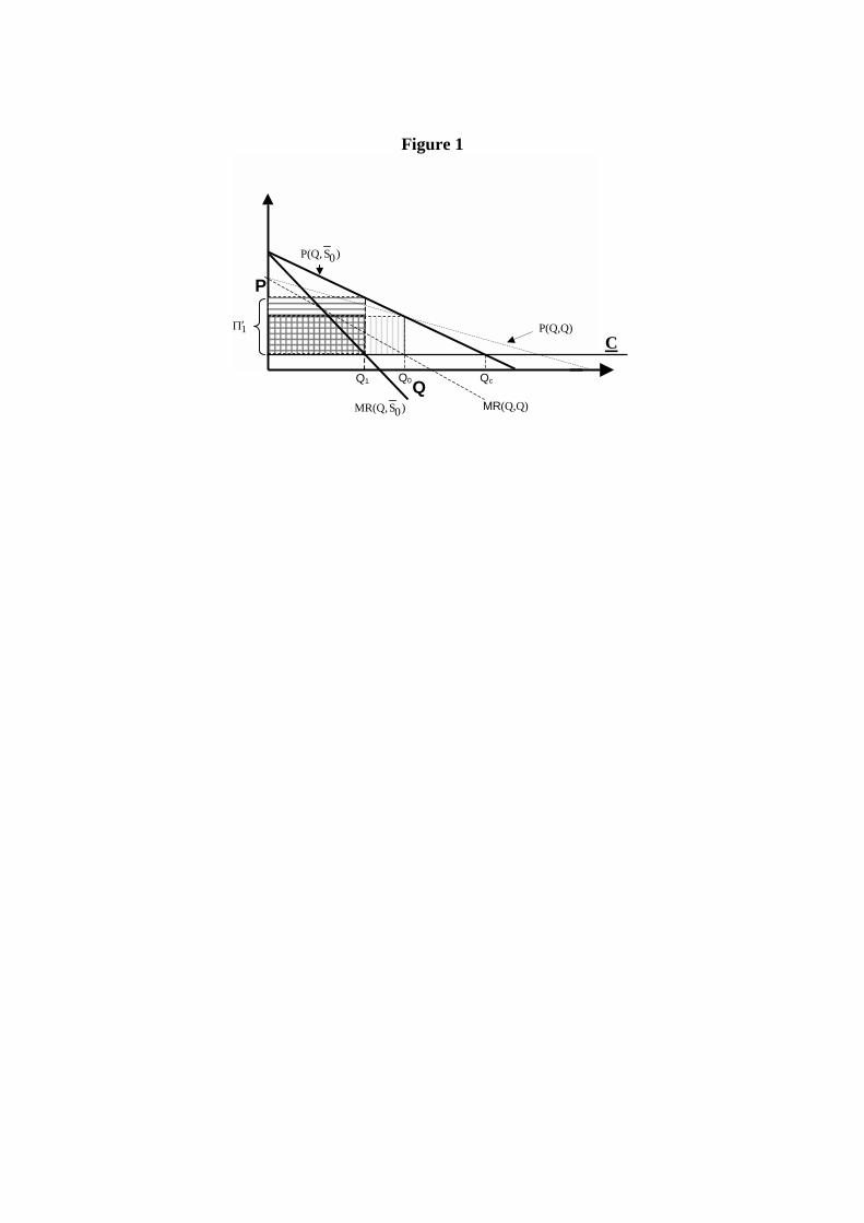
Figure 1
C
Q
P
P(Q,Q)
Q0
MR(Q,Q)
1Π′
Q1
)0SP(Q,
)0SMR(Q,
Qc

Q
S
RF
RC
QE
Figure 2

Figure 3
S
ppQS
ppQ0

Figure 4
Π
0
20
40
60
icΠ
2 4 6 8 10
c
nsΠ
ppΠ

Figure 5
n-1
nppfQ
2 0
2
4
6
8
10
12
14
16
18
ppfq
nppQ
nppTQ
P
n
4 6 8
10 C

Figure 6
n-1
1ppfQ
P
0
2
4
6
8
10
12
14
16
18
1ppTQ
1ppfq
1ppQ
2 4 6 8
10 C
Figure 7
2 4 6 8 10 0 c
Π
20
40
60
nsΠ
ppΠ
1ppΠ
nppΠicΠ

icn
nppn1ppn
Figure 8 Number of Firms
n
1
1.5
2
ppns nn =
0.5
2 4 0
6 8 10 c
ppQ
nsQ
icQ
1ppQ nppQ
Figure 9 Production by the Leader
2 4 6 8 10 0 c
Q
2
6
12
4
8
10

ppTQ
nsTQ ic
TQ
1ppTQ
nppTQ
Figure 10 Market Size
2 4 6 8 100 c
T
2
6
12
4
8
10
18
16
14
Q

ppP
nsP
icP
1ppP
nppP
Figure 11 Price
2 4 6 8 100 c
P
2
6
4
8
10

Table 1 Preference order e c
nsicpp == 32
≤e c=0
nsicpp =f 3
2≤e 0<c<a
nsppic =f 1
32
<< e c=0
nsppic ff 1
32
<< e 2
2831044225240
−
−+−+−+−
<<e
aeeeeeec
nsicpp ff 1
32
<< e ac
e
aeeeeee<<
−
−+−+−+−
2
283104422524

Table 2 Profits
nsΠ ( )
44.110 2c−
ppΠ ( )28.1
10 2c−
icΠ
( )
≤
<−
6.667 if-10 1.25
6676 if441
211010
2 cc
. c .
c).(
nppΠ
( )
≤
<≤−
<−
cc
.c .
c).(
.c c
6.667 if -10 1.25
66761667.4 if441
211010
16674 if28.1
)8.010(
2
2
1ppΠ ( )( )
( )
4.0
122
61
3
4004824412
3 1001226843227120014423241
: where6.667 if -10 1.25
66761.6 if 441
211010
16 if3330
2020102010
2
2
1
21
333
−−=
+−=
+−−−+−=
≤
<≤−
<
−
+−−−
*J
*J
c
*J*J
cc.*J
)cc.c.)(cc.(*J
cc
.c .
c).(
.c
cJJ
cJ.
JJ.c.J.c
*
**
***
Recommended