Convolutional Neural Networks
Computer Vision
Jia-Bin Huang, Virginia Tech

Today’s class
• Overview
• Convolutional Neural Network (CNN)
• Training CNN
• Understanding and Visualizing CNN
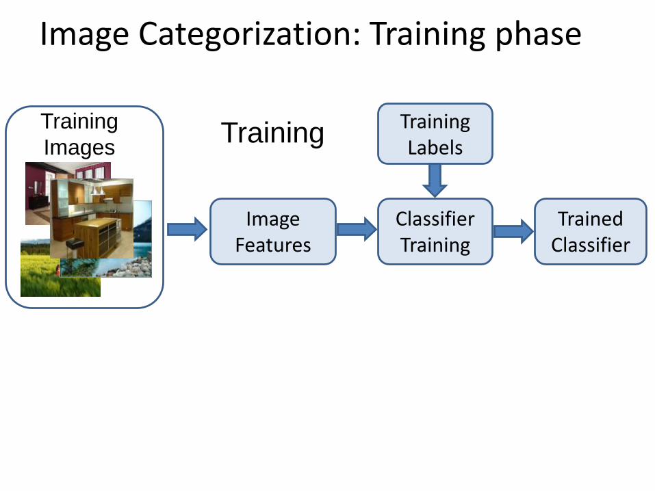
Image Categorization: Training phase
Training Labels
Training
Images
Classifier Training
Training
Image Features
Trained Classifier
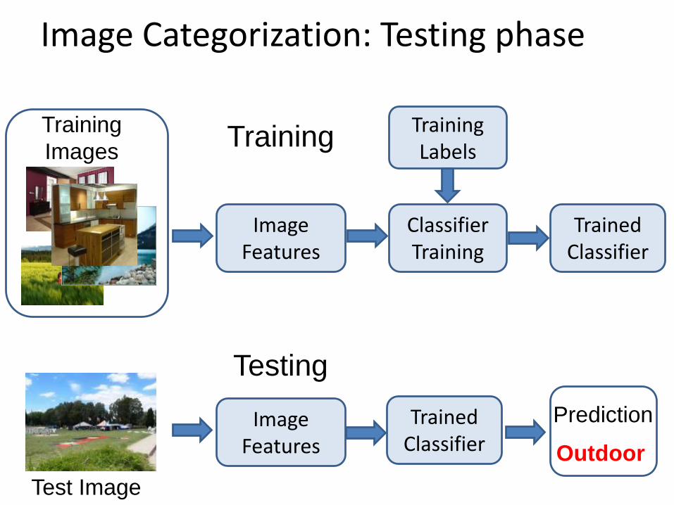
Image Categorization: Testing phase
Training Labels
Training
Images
Classifier Training
Training
Image Features
Trained Classifier
Image Features
Testing
Test Image
Outdoor
PredictionTrained Classifier
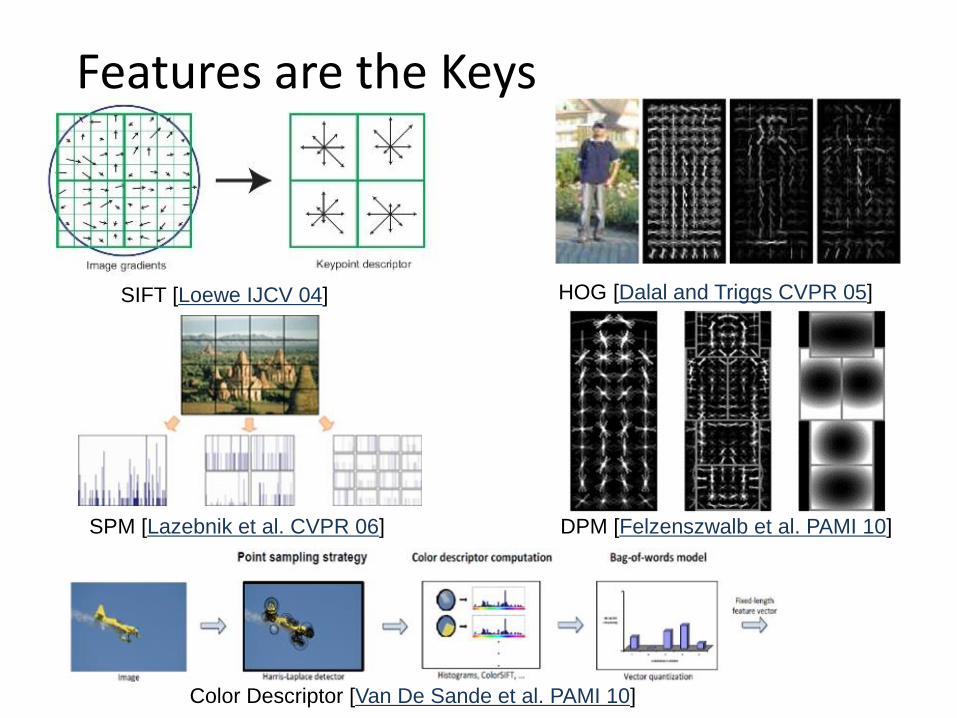
Features are the Keys
SIFT [Loewe IJCV 04] HOG [Dalal and Triggs CVPR 05]
SPM [Lazebnik et al. CVPR 06] DPM [Felzenszwalb et al. PAMI 10]
Color Descriptor [Van De Sande et al. PAMI 10]
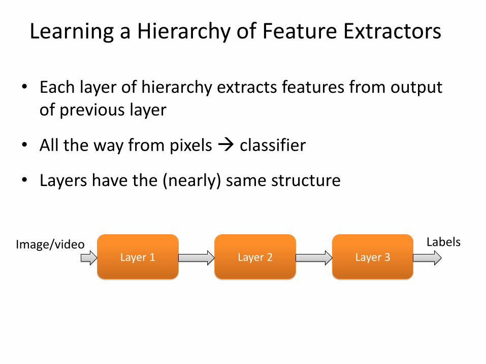
• Each layer of hierarchy extracts features from output of previous layer
• All the way from pixels classifier
• Layers have the (nearly) same structure
Learning a Hierarchy of Feature Extractors
Layer 1 Layer 2 Layer 3Image/video Labels

Biological neuron and Perceptrons
A biological neuron An artificial neuron (Perceptron)
- a linear classifier
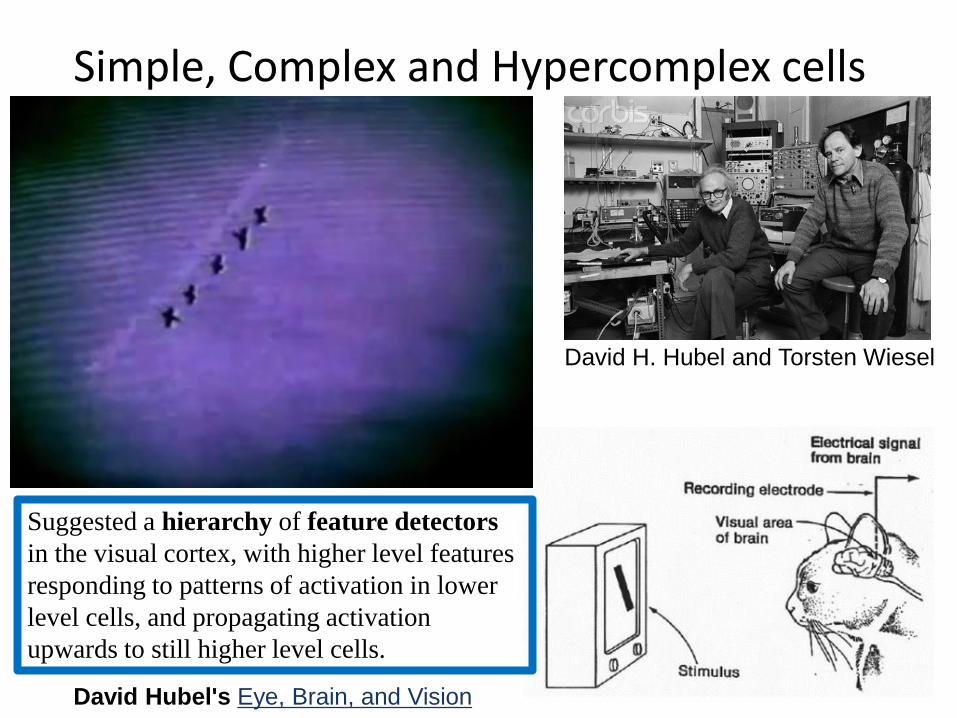
Simple, Complex and Hypercomplex cells
David H. Hubel and Torsten Wiesel
David Hubel's Eye, Brain, and Vision
Suggested a hierarchy of feature detectors
in the visual cortex, with higher level features
responding to patterns of activation in lower
level cells, and propagating activation
upwards to still higher level cells.
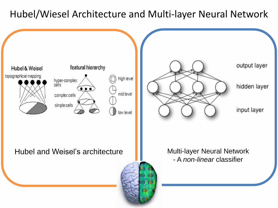
Hubel/Wiesel Architecture and Multi-layer Neural Network
Hubel and Weisel’s architecture Multi-layer Neural Network
- A non-linear classifier

Multi-layer Neural Network
• A non-linear classifier
• Training: find network weights w to minimize the error between true training labels 𝑦𝑖 and estimated labels 𝑓𝒘 𝒙𝒊
• Minimization can be done by gradient descent provided 𝑓 is differentiable
• This training method is called back-propagation
Convolutional Neural Networks
• Also known as CNN, ConvNet, DCN
• CNN = a multi-layer neural network with
1. Local connectivity
2. Weight sharing
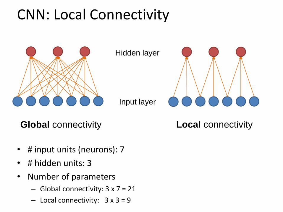
CNN: Local Connectivity
• # input units (neurons): 7
• # hidden units: 3
• Number of parameters– Global connectivity: 3 x 7 = 21
– Local connectivity: 3 x 3 = 9
Input layer
Hidden layer
Global connectivity Local connectivity

CNN: Weight Sharing
Input layer
Hidden layer
• # input units (neurons): 7
• # hidden units: 3
• Number of parameters– Without weight sharing: 3 x 3 = 9
– With weight sharing : 3 x 1 = 3
w1
w2
w3
w4
w5
w6
w7
w8
w9
Without weight sharing With weight sharing
w1
w2
w3 w1
w2
w3
w1
w2
w3
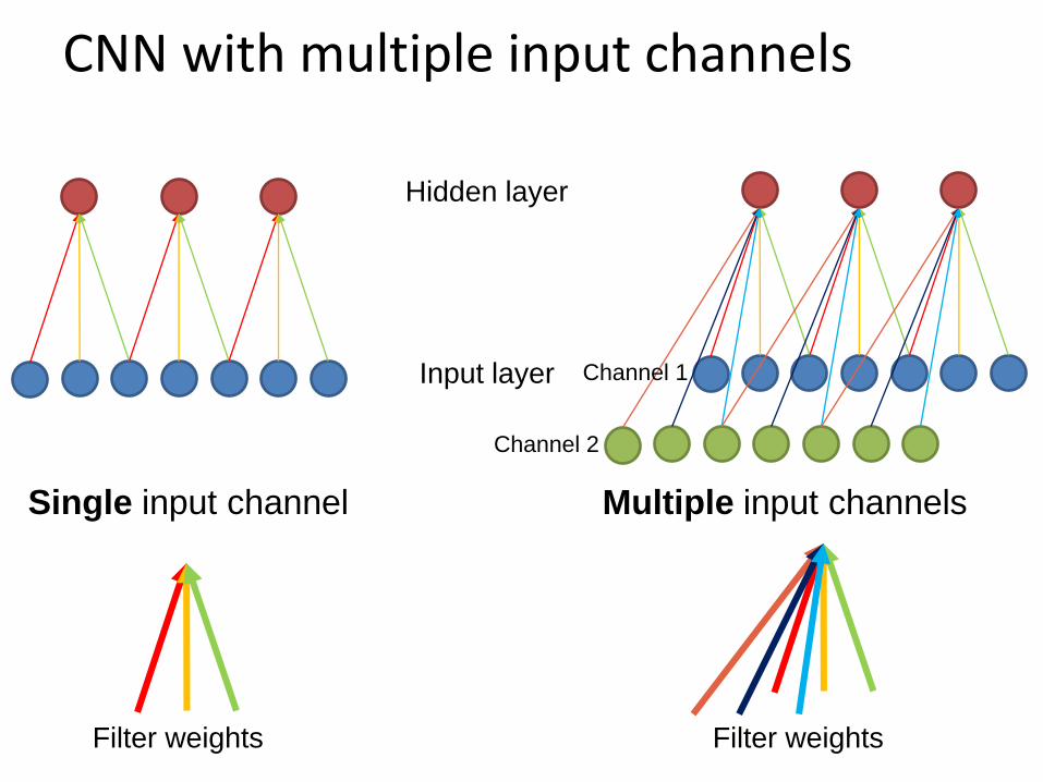
CNN with multiple input channels
Input layer
Hidden layer
Single input channel Multiple input channels
Channel 2
Channel 1
Filter weights Filter weights
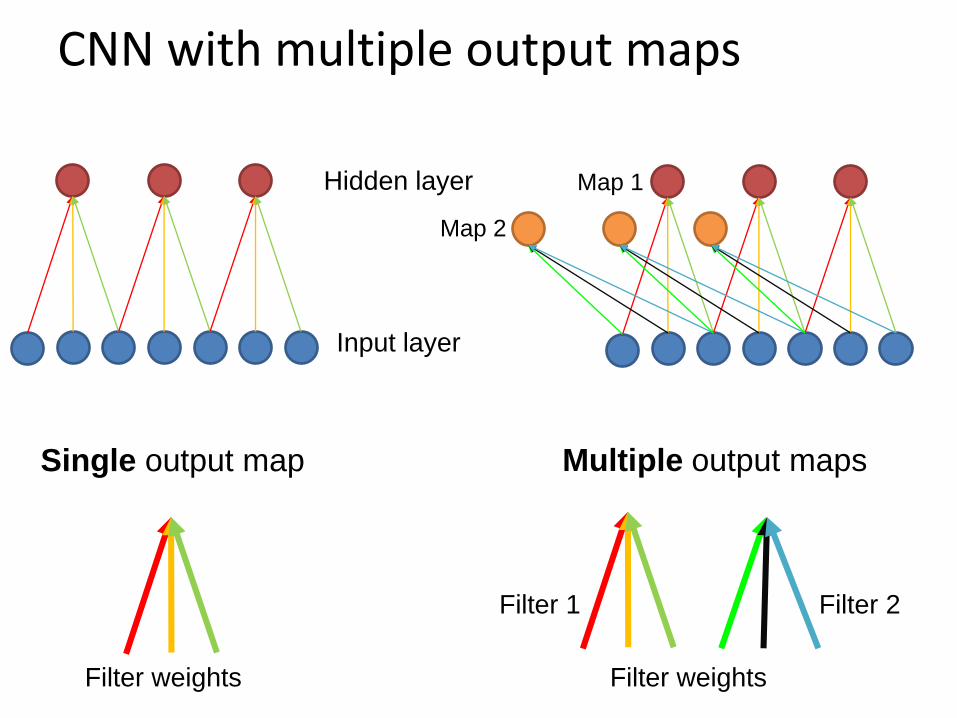
CNN with multiple output maps
Input layer
Hidden layer
Single output map Multiple output maps
Filter weights
Map 1
Map 2
Filter 1 Filter 2
Filter weights

Putting them together
• Local connectivity
• Weight sharing
• Handling multiple input channels
• Handling multiple output maps
Image credit: A. Karpathy# output (activation) maps # input channels
Local connectivity
Weight sharing
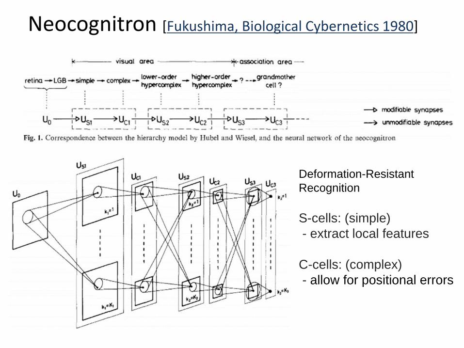
Neocognitron [Fukushima, Biological Cybernetics 1980]
Deformation-Resistant
Recognition
S-cells: (simple)
- extract local features
C-cells: (complex)
- allow for positional errors

LeNet [LeCun et al. 1998]
Gradient-based learning applied to document recognition [LeCun, Bottou, Bengio, Haffner 1998] LeNet-1 from 1993
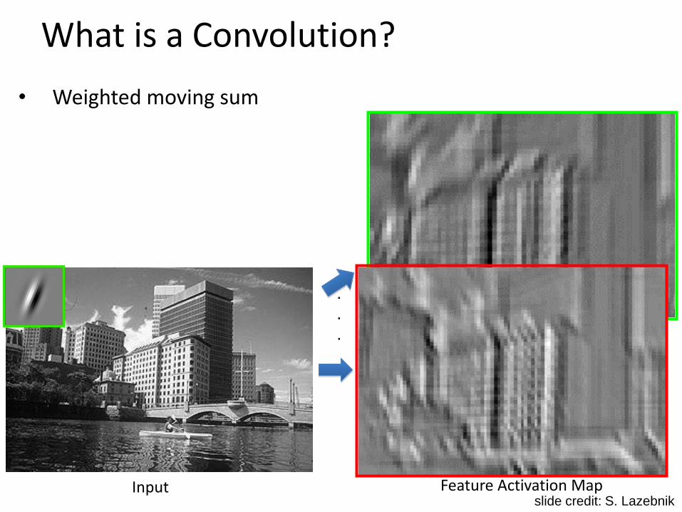
What is a Convolution?
• Weighted moving sum
Input Feature Activation Map
.
.
.
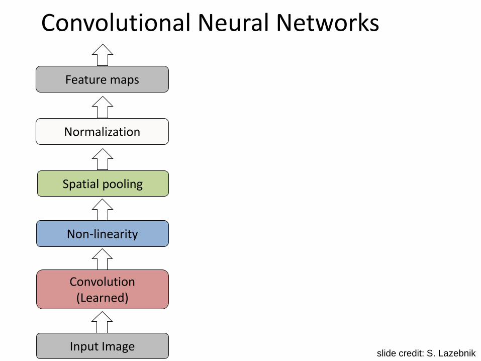
slide credit: S. Lazebnik

Input Image
Convolution (Learned)
Non-linearity
Spatial pooling
Normalization
Convolutional Neural Networks
Feature maps
slide credit: S. Lazebnik
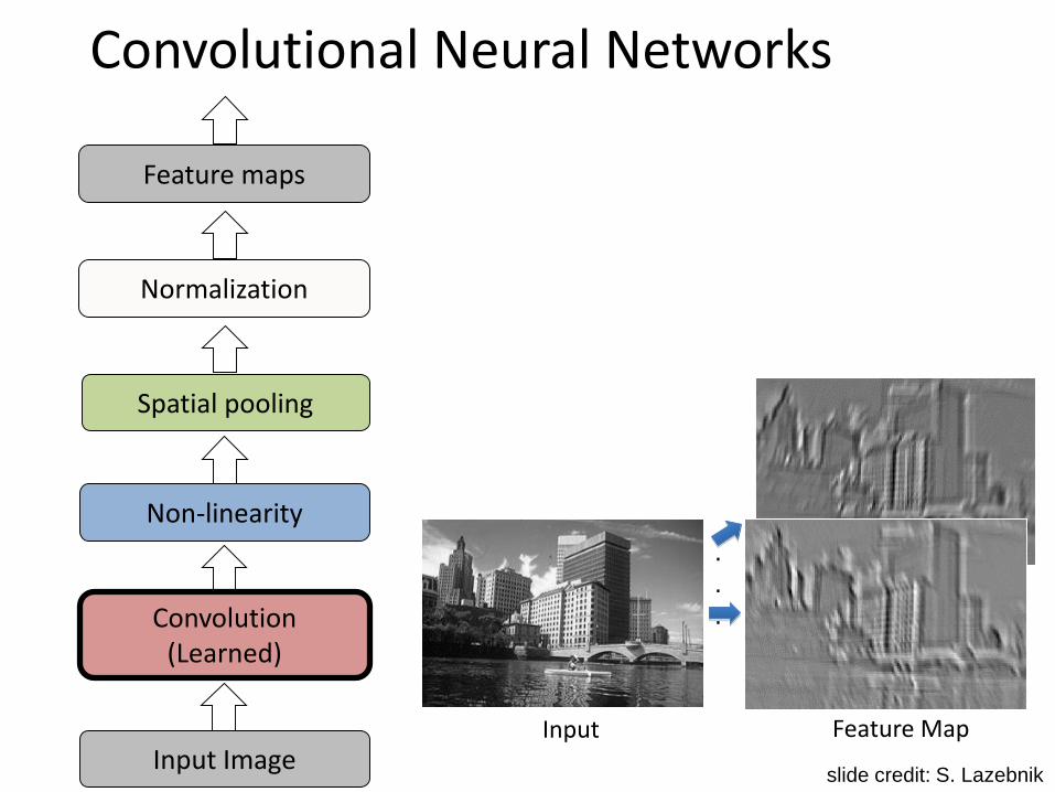
Input Image
Convolution (Learned)
Non-linearity
Spatial pooling
Normalization
Feature maps
Input Feature Map
.
.
.
Convolutional Neural Networks
slide credit: S. Lazebnik
Input Image
Convolution (Learned)
Non-linearity
Spatial pooling
Normalization
Feature maps
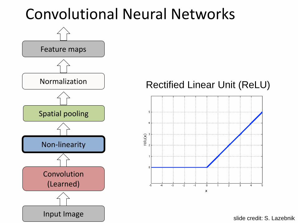
Convolutional Neural Networks
Rectified Linear Unit (ReLU)
slide credit: S. Lazebnik

Input Image
Convolution (Learned)
Non-linearity
Spatial pooling
Normalization
Feature maps
Max pooling
Convolutional Neural Networks
slide credit: S. Lazebnik
Max-pooling: a non-linear down-sampling
Provide translation invariance
Input Image
Convolution (Learned)
Non-linearity
Spatial pooling
Normalization
Feature maps
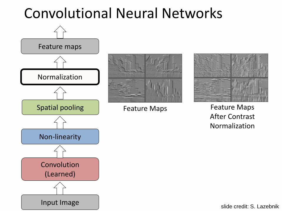
Feature Maps Feature MapsAfter Contrast Normalization
Convolutional Neural Networks
slide credit: S. Lazebnik
Input Image
Convolution (Learned)
Non-linearity
Spatial pooling
Normalization
Feature maps
Convolutional Neural Networks
slide credit: S. Lazebnik
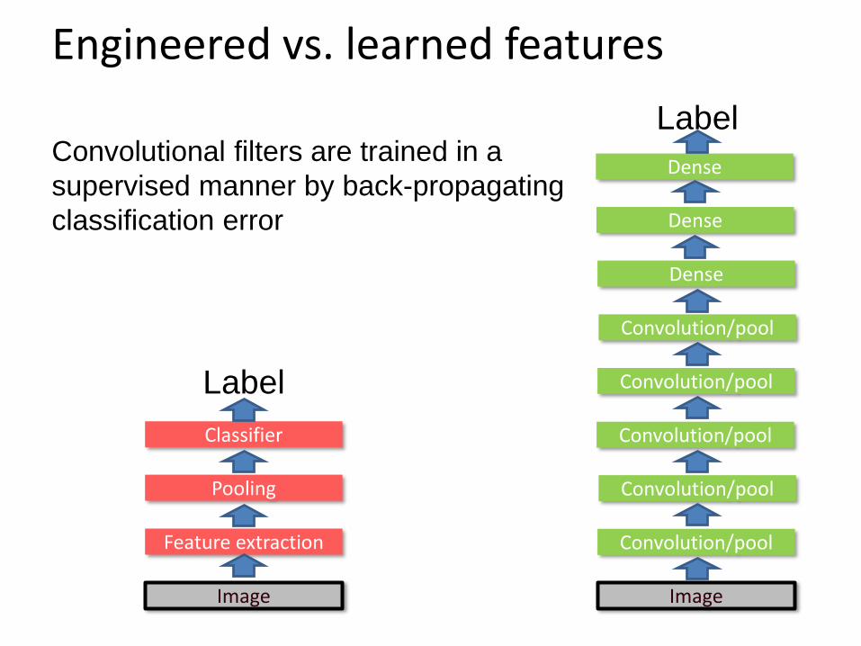
Engineered vs. learned features
Image
Feature extraction
Pooling
Classifier
Label
Image
Convolution/pool
Convolution/pool
Convolution/pool
Convolution/pool
Convolution/pool
Dense
Dense
Dense
LabelConvolutional filters are trained in a
supervised manner by back-propagating
classification error
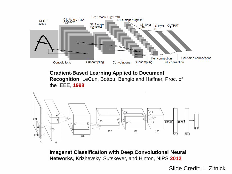
Imagenet Classification with Deep Convolutional Neural
Networks, Krizhevsky, Sutskever, and Hinton, NIPS 2012
Gradient-Based Learning Applied to Document
Recognition, LeCun, Bottou, Bengio and Haffner, Proc. of
the IEEE, 1998
Slide Credit: L. Zitnick
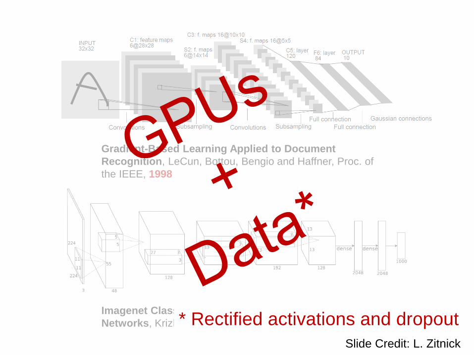
Imagenet Classification with Deep Convolutional Neural
Networks, Krizhevsky, Sutskever, and Hinton, NIPS 2012
Gradient-Based Learning Applied to Document
Recognition, LeCun, Bottou, Bengio and Haffner, Proc. of
the IEEE, 1998
* Rectified activations and dropout
Slide Credit: L. Zitnick

SIFT Descriptor
Image Pixels
Apply gradient filters
Spatial pool
(Sum)
Normalize to unit length
Feature Vector
Lowe [IJCV 2004]

SIFT Descriptor
Image Pixels Apply
oriented filters
Spatial pool
(Sum)
Normalize to unit length
Feature Vector
Lowe [IJCV 2004]
slide credit: R. Fergus

Spatial Pyramid Matching
SIFTFeatures
Filter with Visual Words
Multi-scalespatial pool
(Sum)
Max
Classifier
Lazebnik, Schmid,
Ponce [CVPR 2006]
slide credit: R. Fergus
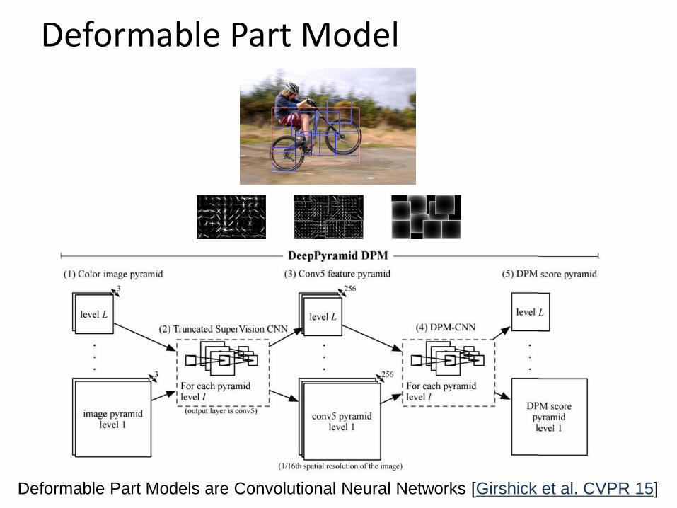
Deformable Part Model
Deformable Part Models are Convolutional Neural Networks [Girshick et al. CVPR 15]
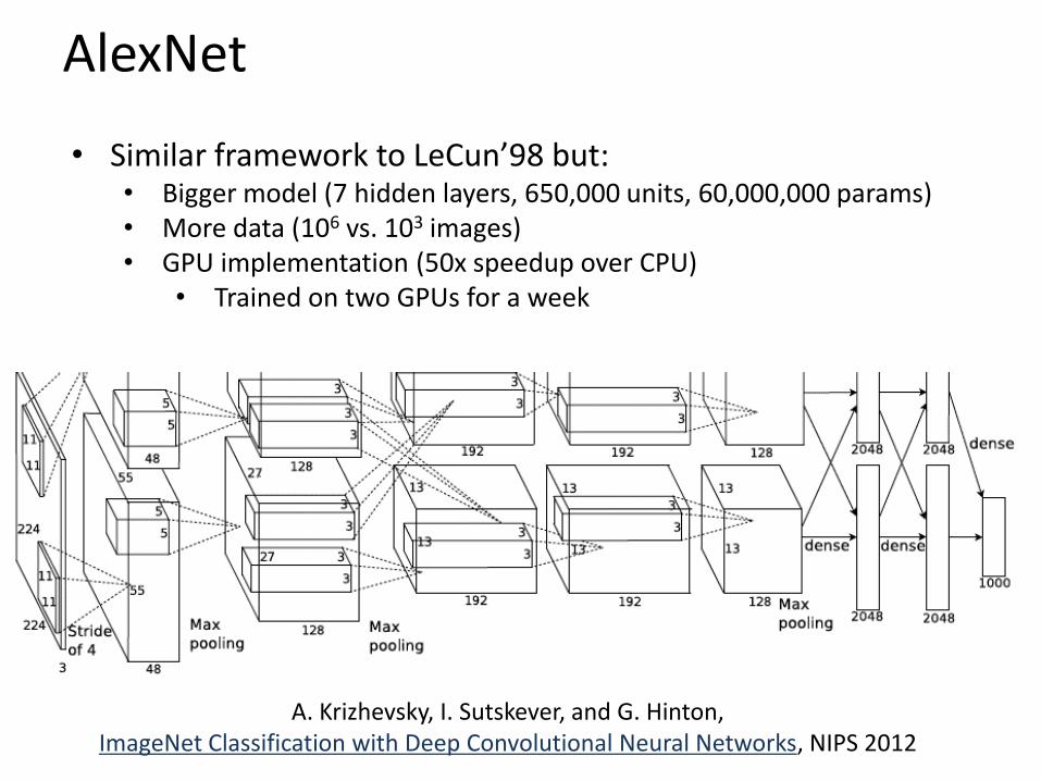
AlexNet
• Similar framework to LeCun’98 but:• Bigger model (7 hidden layers, 650,000 units, 60,000,000 params)• More data (106 vs. 103 images)• GPU implementation (50x speedup over CPU)
• Trained on two GPUs for a week
A. Krizhevsky, I. Sutskever, and G. Hinton, ImageNet Classification with Deep Convolutional Neural Networks, NIPS 2012
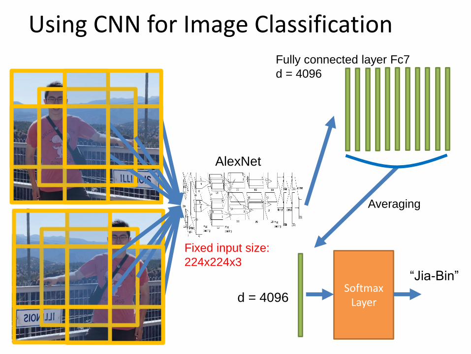
Using CNN for Image Classification
AlexNet
Fully connected layer Fc7
d = 4096
d = 4096
Averaging
SoftmaxLayer
“Jia-Bin”
Fixed input size:
224x224x3

Progress on ImageNet
2012
AlexNet
2013
ZF
2014
VGG
2014
GoogLeNet
2015
ResNet
2016
GoogLeNet-v4
15
10
5
ImageNet Image Classification Top5
Error
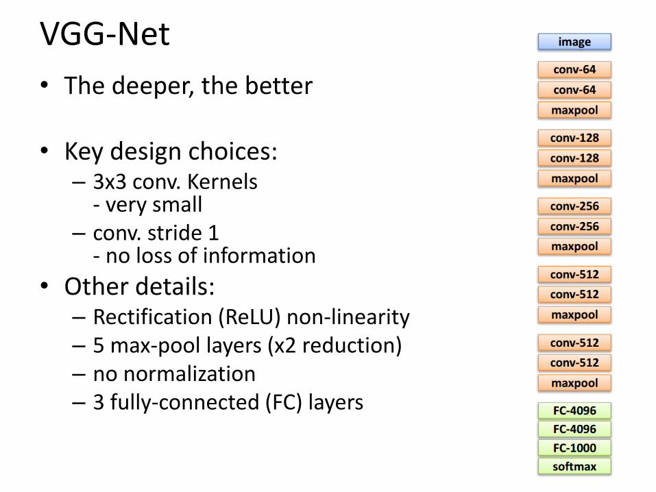
VGG-Net
• The deeper, the better
• Key design choices:– 3x3 conv. Kernels
- very small– conv. stride 1
- no loss of information
• Other details:– Rectification (ReLU) non-linearity – 5 max-pool layers (x2 reduction)– no normalization– 3 fully-connected (FC) layers

VGG-Net
• Why 3x3 layers?
– Stacked conv. layers have a large receptive field
– two 3x3 layers – 5x5 receptive field
– three 3x3 layers – 7x7 receptive field
• More non-linearity
– Less parameters to learn
– ~140M per net

ResNet
• Can we just increase the #layer?
• How can we train very deep network?- Residual learning

DenseNet
• Shorter connections (like ResNet) help
• Why not just connect them all?
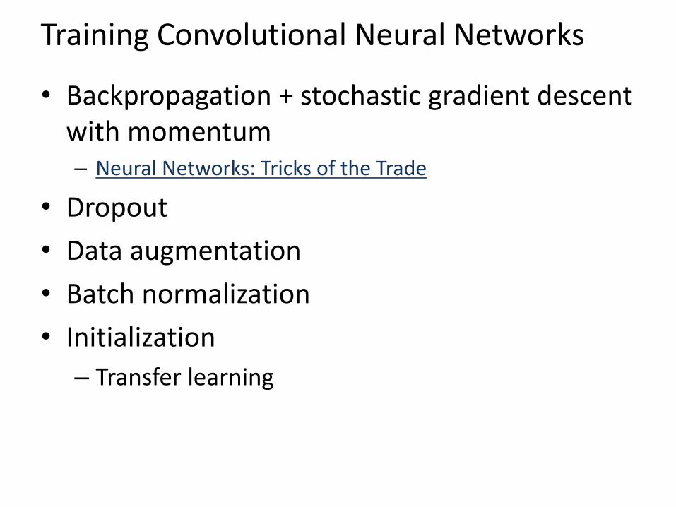
Training Convolutional Neural Networks
• Backpropagation + stochastic gradient descent with momentum – Neural Networks: Tricks of the Trade
• Dropout
• Data augmentation
• Batch normalization
• Initialization
– Transfer learning

Training CNN with gradient descent
• A CNN as composition of functions𝑓𝒘 𝒙 = 𝑓𝐿(… (𝑓2 𝑓1 𝒙;𝒘1 ; 𝒘2 … ;𝒘𝐿)
• Parameters𝒘 = (𝒘𝟏, 𝒘𝟐, …𝒘𝑳)
• Empirical loss function
𝐿 𝒘 =1
𝑛
𝑖
𝑙(𝑧𝑖 , 𝑓𝒘(𝒙𝒊))
• Gradient descent
𝒘𝒕+𝟏 = 𝒘𝒕 − 𝜂𝑡𝜕𝒇
𝜕𝒘(𝒘𝒕)
Learning rate GradientOld weight
New weight
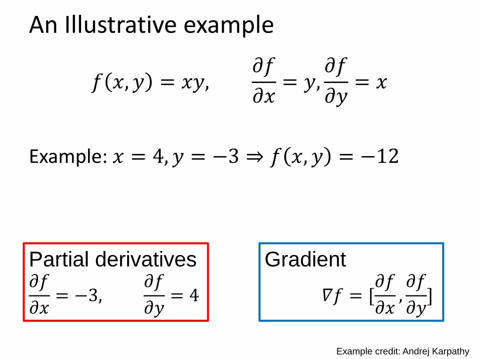
An Illustrative example
𝑓 𝑥, 𝑦 = 𝑥𝑦,𝜕𝑓
𝜕𝑥= 𝑦,
𝜕𝑓
𝜕𝑦= 𝑥
Example: 𝑥 = 4, 𝑦 = −3 ⇒ 𝑓 𝑥, 𝑦 = −12
Example credit: Andrej Karpathy
Partial derivatives𝜕𝑓
𝜕𝑥= −3,
𝜕𝑓
𝜕𝑦= 4
Gradient
𝛻𝑓 = [𝜕𝑓
𝜕𝑥,𝜕𝑓
𝜕𝑦]
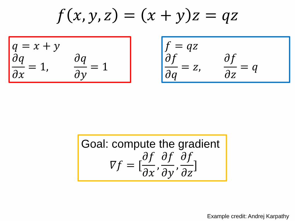
𝑓 𝑥, 𝑦, 𝑧 = 𝑥 + 𝑦 𝑧 = 𝑞𝑧
Example credit: Andrej Karpathy
𝑞 = 𝑥 + 𝑦𝜕𝑞
𝜕𝑥= 1,
𝜕𝑞
𝜕𝑦= 1
𝑓 = 𝑞𝑧𝜕𝑓
𝜕𝑞= 𝑧,
𝜕𝑓
𝜕𝑧= 𝑞
Goal: compute the gradient
𝛻𝑓 = [𝜕𝑓
𝜕𝑥,𝜕𝑓
𝜕𝑦,𝜕𝑓
𝜕𝑧]

𝑓 𝑥, 𝑦, 𝑧 = 𝑥 + 𝑦 𝑧 = 𝑞𝑧
Example credit: Andrej Karpathy
𝑓 = 𝑞𝑧𝜕𝑓
𝜕𝑞= 𝑧,
𝜕𝑓
𝜕𝑧= 𝑞
Chain rule:𝜕𝑓
𝜕𝑥=
𝜕𝑓
𝜕𝑞
𝜕𝑞
𝜕𝑥
𝑞 = 𝑥 + 𝑦𝜕𝑞
𝜕𝑥= 1,
𝜕𝑞
𝜕𝑦= 1

Backpropagation (recursive chain rule)
𝑞
𝑤1
𝑤2
𝑤𝑛
𝜕𝑓
𝜕𝑞
𝜕𝑓
𝜕𝑤𝑖=
𝜕𝑞
𝜕𝑤𝑖
𝜕𝑓
𝜕𝑞
Gate gradientLocal gradient
The gate receives this during backpropCan be computed during forward pass

Dropout
Dropout: A simple way to prevent neural networks from overfitting [Srivastava JMLR 2014]
Intuition: successful conspiracies
• 50 people planning a conspiracy
• Strategy A: plan a big conspiracy involving 50 people
• Likely to fail. 50 people need to play their parts correctly.
• Strategy B: plan 10 conspiracies each involving 5 people
• Likely to succeed!
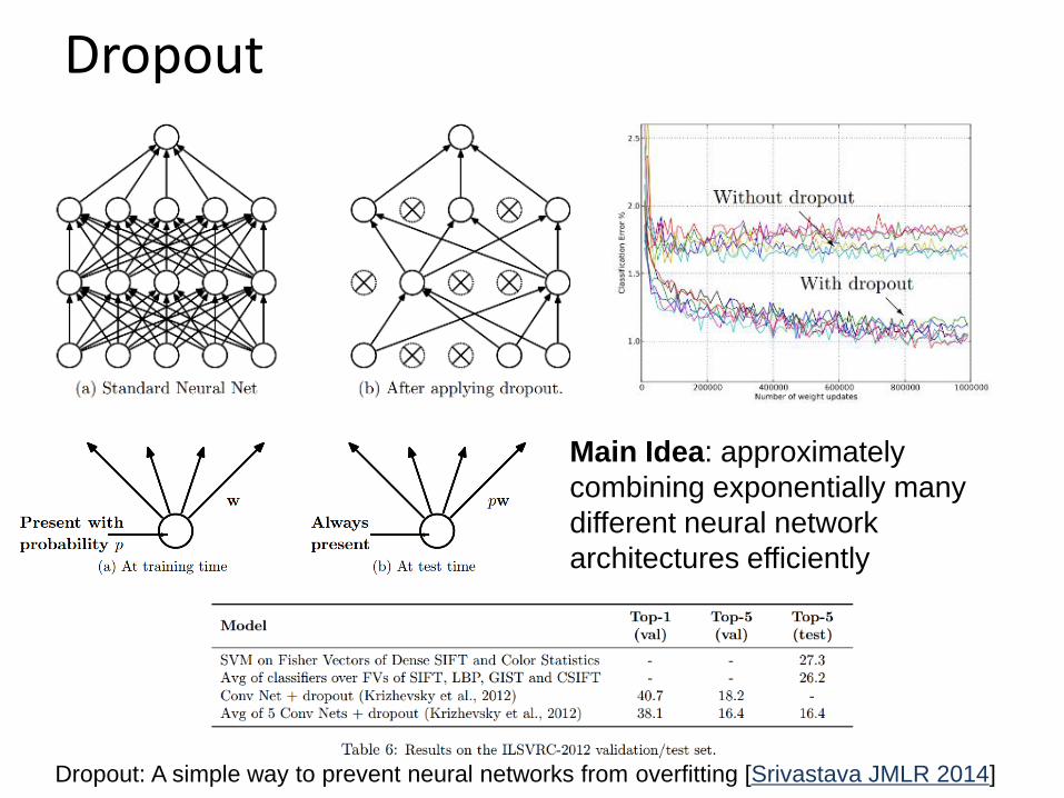
Dropout
Dropout: A simple way to prevent neural networks from overfitting [Srivastava JMLR 2014]
Main Idea: approximately
combining exponentially many
different neural network
architectures efficiently

Data Augmentation (Jittering)
• Create virtual training samples
– Horizontal flip
– Random crop
– Color casting
– Geometric distortion
Deep Image [Wu et al. 2015]
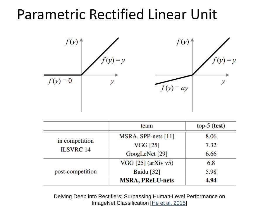
Parametric Rectified Linear Unit
Delving Deep into Rectifiers: Surpassing Human-Level Performance on
ImageNet Classification [He et al. 2015]

Swish
The Swish activation function First derivatives of Swish
https://arxiv.org/abs/1710.05941
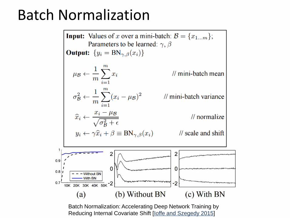
Batch Normalization
Batch Normalization: Accelerating Deep Network Training by
Reducing Internal Covariate Shift [Ioffe and Szegedy 2015]

Understanding and Visualizing CNN
• Find images that maximize some class scores
• Individual neuron activation
• Breaking CNNs
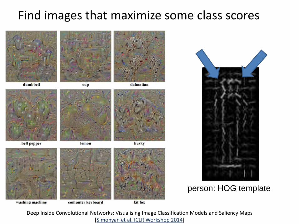
Find images that maximize some class scores
person: HOG template
Deep Inside Convolutional Networks: Visualising Image Classification Models and Saliency Maps [Simonyan et al. ICLR Workshop 2014]

Individual Neuron Activation
RCNN [Girshick et al. CVPR 2014]

Individual Neuron Activation
RCNN [Girshick et al. CVPR 2014]

Individual Neuron Activation
RCNN [Girshick et al. CVPR 2014]

Map activation back to the input pixel space
• What input pattern originally caused a given activation in the feature maps?
Visualizing and Understanding Convolutional Networks [Zeiler and Fergus, ECCV 2014]

Layer 1
Visualizing and Understanding Convolutional Networks [Zeiler and Fergus, ECCV 2014]
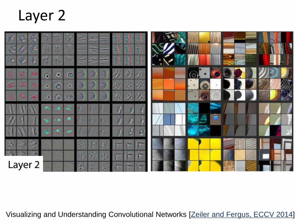
Layer 2
Visualizing and Understanding Convolutional Networks [Zeiler and Fergus, ECCV 2014]

Layer 3
Visualizing and Understanding Convolutional Networks [Zeiler and Fergus, ECCV 2014]
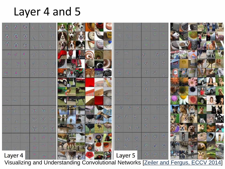
Layer 4 and 5
Visualizing and Understanding Convolutional Networks [Zeiler and Fergus, ECCV 2014]
Deep learning library
• TensorFlow
– Research + Production
• PyTorch
– Research
• Caffe2
– Production

Things to remember
• Convolutional neural networks
– A cascade of conv + ReLU + pool
– Representation learning
– Advanced architectures
– Tricks for training CNN
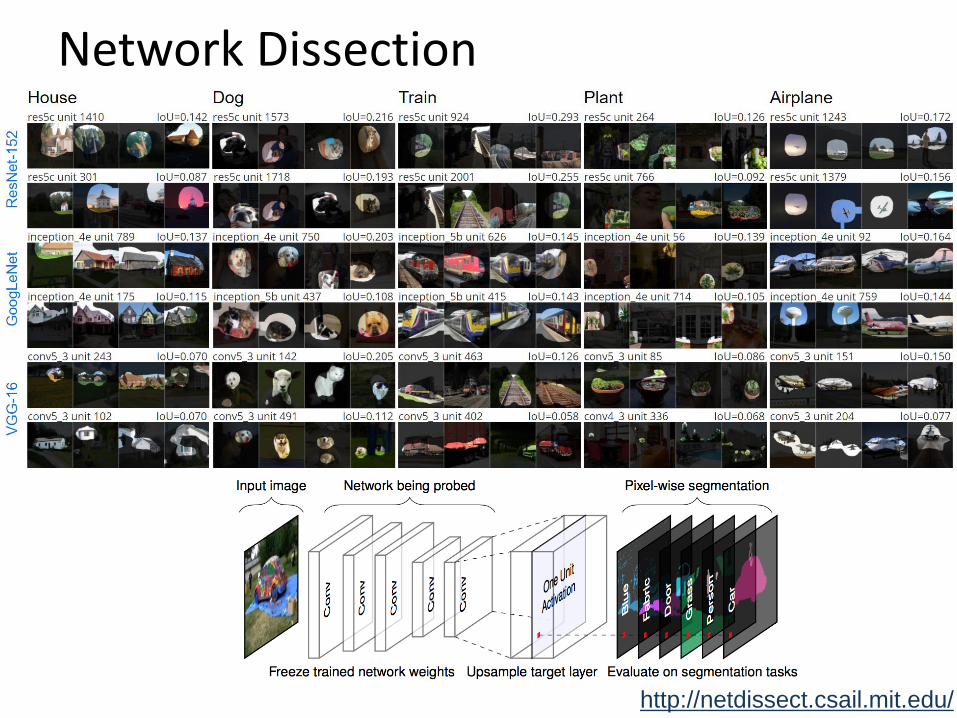
• Visualizing CNN
– Activation
– Dissection
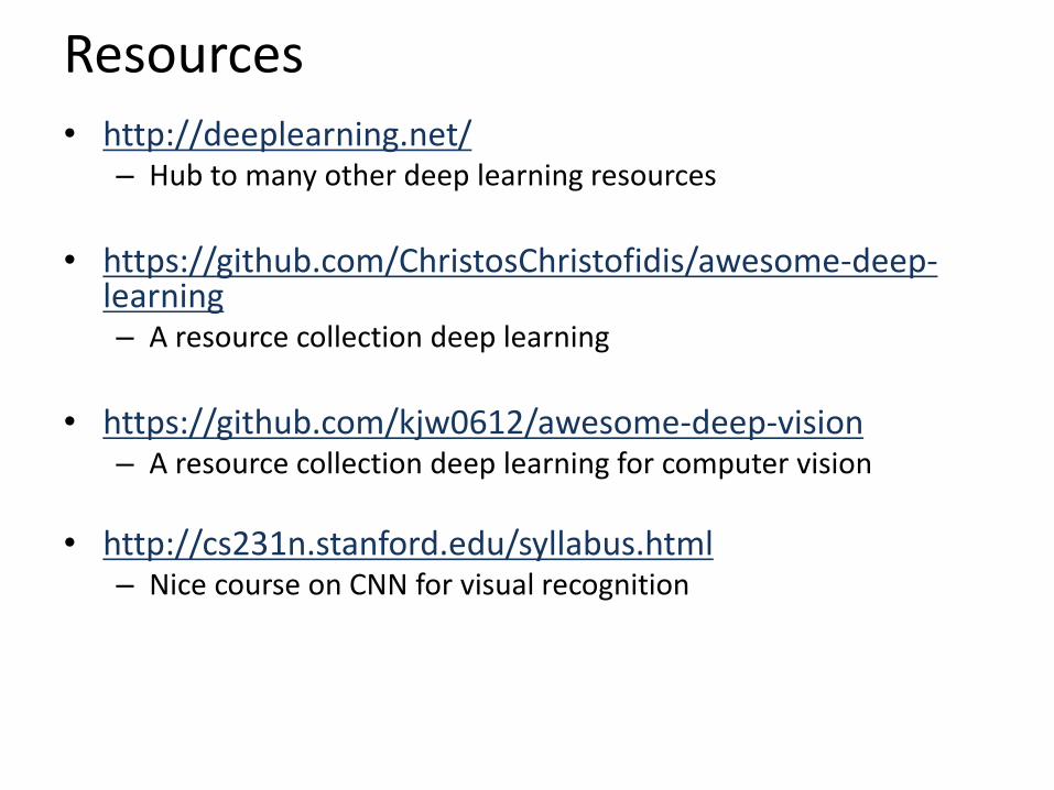
Resources
• http://deeplearning.net/– Hub to many other deep learning resources
• https://github.com/ChristosChristofidis/awesome-deep-learning– A resource collection deep learning
• https://github.com/kjw0612/awesome-deep-vision– A resource collection deep learning for computer vision
• http://cs231n.stanford.edu/syllabus.html– Nice course on CNN for visual recognition

Things to remember
• Overview– Neuroscience, Perceptron, multi-layer neural
networks
• Convolutional neural network (CNN)– Convolution, nonlinearity, max pooling– CNN for classification and beyond
• Understanding and visualizing CNN– Find images that maximize some class scores;
visualize individual neuron activation, input pattern and images; breaking CNNs
• Training CNN– Dropout; data augmentation; batch normalization;
transfer learning
Recommended