Convex Optimization(EE227A: UC Berkeley)
Lecture 3(Convex sets and functions)
29 Jan, 2013
◦
Suvrit Sra

Course organization
http://people.kyb.tuebingen.mpg.de/suvrit/teach/ee227a/
Relevant texts / references:
♥ Convex optimization – Boyd & Vandenberghe (BV)♥ Introductory lectures on convex optimisation – Nesterov♥ Nonlinear programming – Bertsekas♥ Convex Analysis – Rockafellar♥ Numerical optimization – Nocedal & Wright♥ Lectures on modern convex optimization – Nemirovski♥ Optimization for Machine Learning – Sra, Nowozin, Wright
Instructor: Suvrit Sra ([email protected])(Max Planck Institute for Intelligent Systems, Tubingen, Germany)
HW + Quizzes (40%); Midterm (30%); Project (30%)
TA Office hours to be posted soon
I don’t have an office yet
If you email me, please put EE227A in Subject:
2 / 42
Linear algebra recap
3 / 42

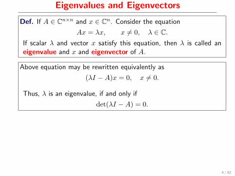
Eigenvalues and Eigenvectors
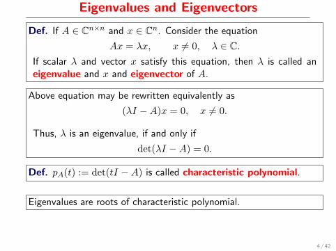
Def. If A ∈ Cn×n and x ∈ Cn. Consider the equation
Ax = λx, x 6= 0, λ ∈ C.If scalar λ and vector x satisfy this equation, then λ is called aneigenvalue and x and eigenvector of A.
Above equation may be rewritten equivalently as
(λI −A)x = 0, x 6= 0.
Thus, λ is an eigenvalue, if and only if
det(λI −A) = 0.
Def. pA(t) := det(tI −A) is called characteristic polynomial.
Eigenvalues are roots of characteristic polynomial.
4 / 42
Eigenvalues and Eigenvectors
Def. If A ∈ Cn×n and x ∈ Cn. Consider the equation
Ax = λx, x 6= 0, λ ∈ C.If scalar λ and vector x satisfy this equation, then λ is called aneigenvalue and x and eigenvector of A.
Above equation may be rewritten equivalently as
(λI −A)x = 0, x 6= 0.
Thus, λ is an eigenvalue, if and only if
det(λI −A) = 0.
Def. pA(t) := det(tI −A) is called characteristic polynomial.
Eigenvalues are roots of characteristic polynomial.
4 / 42
Eigenvalues and Eigenvectors
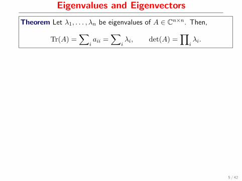
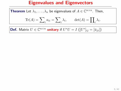
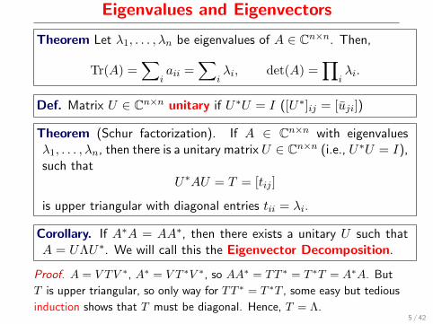
Theorem Let λ1, . . . , λn be eigenvalues of A ∈ Cn×n. Then,
Tr(A) =∑
iaii =
∑iλi, det(A) =
∏iλi.
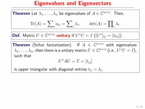
Def. Matrix U ∈ Cn×n unitary if U∗U = I ([U∗]ij = [uji])
Theorem (Schur factorization). If A ∈ Cn×n with eigenvaluesλ1, . . . , λn, then there is a unitary matrix U ∈ Cn×n (i.e., U∗U = I),such that
U∗AU = T = [tij ]
is upper triangular with diagonal entries tii = λi.
Corollary. If A∗A = AA∗, then there exists a unitary U such thatA = UΛU∗. We will call this the Eigenvector Decomposition.
Proof. A = V TV ∗, A∗ = V T ∗V ∗, so AA∗ = TT ∗ = T ∗T = A∗A. But
T is upper triangular, so only way for TT ∗ = T ∗T , some easy but tedious
induction shows that T must be diagonal. Hence, T = Λ.
5 / 42
Eigenvalues and Eigenvectors
Theorem Let λ1, . . . , λn be eigenvalues of A ∈ Cn×n. Then,
Tr(A) =∑
iaii =
∑iλi, det(A) =
∏iλi.
Def. Matrix U ∈ Cn×n unitary if U∗U = I ([U∗]ij = [uji])
Theorem (Schur factorization). If A ∈ Cn×n with eigenvaluesλ1, . . . , λn, then there is a unitary matrix U ∈ Cn×n (i.e., U∗U = I),such that
U∗AU = T = [tij ]
is upper triangular with diagonal entries tii = λi.
Corollary. If A∗A = AA∗, then there exists a unitary U such thatA = UΛU∗. We will call this the Eigenvector Decomposition.
Proof. A = V TV ∗, A∗ = V T ∗V ∗, so AA∗ = TT ∗ = T ∗T = A∗A. But
T is upper triangular, so only way for TT ∗ = T ∗T , some easy but tedious
induction shows that T must be diagonal. Hence, T = Λ.
5 / 42
Eigenvalues and Eigenvectors
Theorem Let λ1, . . . , λn be eigenvalues of A ∈ Cn×n. Then,
Tr(A) =∑
iaii =
∑iλi, det(A) =
∏iλi.
Def. Matrix U ∈ Cn×n unitary if U∗U = I ([U∗]ij = [uji])
Theorem (Schur factorization). If A ∈ Cn×n with eigenvaluesλ1, . . . , λn, then there is a unitary matrix U ∈ Cn×n (i.e., U∗U = I),such that
U∗AU = T = [tij ]
is upper triangular with diagonal entries tii = λi.
Corollary. If A∗A = AA∗, then there exists a unitary U such thatA = UΛU∗. We will call this the Eigenvector Decomposition.
Proof. A = V TV ∗, A∗ = V T ∗V ∗, so AA∗ = TT ∗ = T ∗T = A∗A. But
T is upper triangular, so only way for TT ∗ = T ∗T , some easy but tedious
induction shows that T must be diagonal. Hence, T = Λ.5 / 42
Singular value decomposition
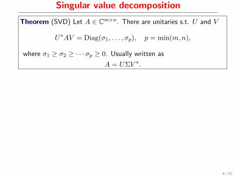
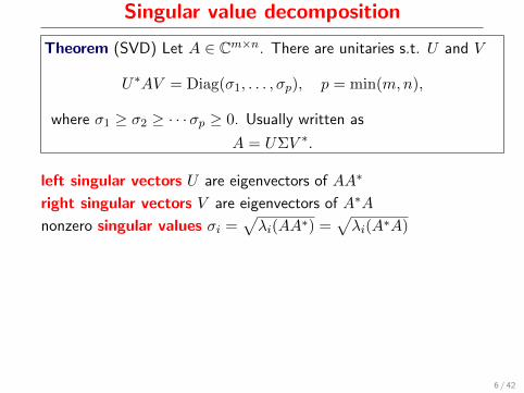
Theorem (SVD) Let A ∈ Cm×n. There are unitaries s.t. U and V
U∗AV = Diag(σ1, . . . , σp), p = min(m,n),
where σ1 ≥ σ2 ≥ · · ·σp ≥ 0. Usually written as
A = UΣV ∗.
left singular vectors U are eigenvectors of AA∗
right singular vectors V are eigenvectors of A∗A
nonzero singular values σi =√λi(AA∗) =
√λi(A∗A)
6 / 42
Singular value decomposition
Theorem (SVD) Let A ∈ Cm×n. There are unitaries s.t. U and V
U∗AV = Diag(σ1, . . . , σp), p = min(m,n),
where σ1 ≥ σ2 ≥ · · ·σp ≥ 0. Usually written as
A = UΣV ∗.
left singular vectors U are eigenvectors of AA∗
right singular vectors V are eigenvectors of A∗A
nonzero singular values σi =√λi(AA∗) =
√λi(A∗A)
6 / 42

Positive definite matrices
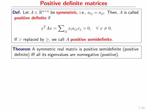
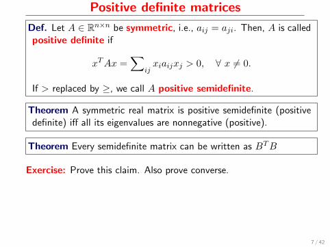
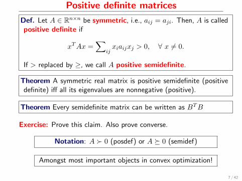
Def. Let A ∈ Rn×n be symmetric, i.e., aij = aji. Then, A is calledpositive definite if
xTAx =∑
ijxiaijxj > 0, ∀ x 6= 0.
If > replaced by ≥, we call A positive semidefinite.
Theorem A symmetric real matrix is positive semidefinite (positivedefinite) iff all its eigenvalues are nonnegative (positive).
Theorem Every semidefinite matrix can be written as BTB
Exercise: Prove this claim. Also prove converse.
Notation: A � 0 (posdef) or A � 0 (semidef)
Amongst most important objects in convex optimization!
7 / 42
Positive definite matrices
Def. Let A ∈ Rn×n be symmetric, i.e., aij = aji. Then, A is calledpositive definite if
xTAx =∑
ijxiaijxj > 0, ∀ x 6= 0.
If > replaced by ≥, we call A positive semidefinite.
Theorem A symmetric real matrix is positive semidefinite (positivedefinite) iff all its eigenvalues are nonnegative (positive).
Theorem Every semidefinite matrix can be written as BTB
Exercise: Prove this claim. Also prove converse.
Notation: A � 0 (posdef) or A � 0 (semidef)
Amongst most important objects in convex optimization!
7 / 42

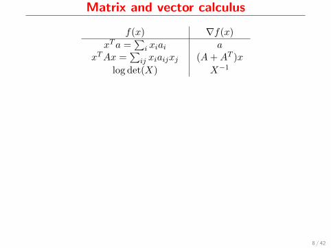
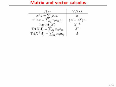
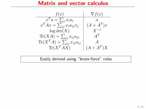
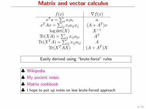
Matrix and vector calculus
f(x) ∇f(x)
xTa =∑
i xiai a
xTAx =∑
ij xiaijxj (A+AT )x
log det(X) X−1
Tr(XA) =∑
ij xijaji AT
Tr(XTA) =∑
ij xijaij A
Tr(XTAX) (A+AT )X
Easily derived using “brute-force” rules
♣ Wikipedia
♣ My ancient notes
♣ Matrix cookbook
♣ I hope to put up notes on less brute-forced approach.
8 / 42

Matrix and vector calculus
f(x) ∇f(x)
xTa =∑
i xiai axTAx =
∑ij xiaijxj (A+AT )x
log det(X) X−1
Tr(XA) =∑
ij xijaji AT
Tr(XTA) =∑
ij xijaij A
Tr(XTAX) (A+AT )X
Easily derived using “brute-force” rules
♣ Wikipedia
♣ My ancient notes
♣ Matrix cookbook
♣ I hope to put up notes on less brute-forced approach.
8 / 42
Convex Sets
9 / 42
Convex sets
10 / 42

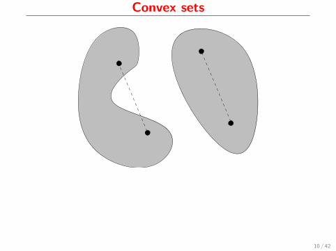
Convex sets
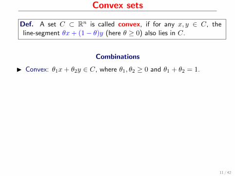
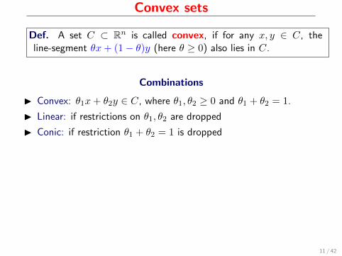
Def. A set C ⊂ Rn is called convex, if for any x, y ∈ C, theline-segment θx+ (1− θ)y (here θ ≥ 0) also lies in C.
Combinations
I Convex: θ1x+ θ2y ∈ C, where θ1, θ2 ≥ 0 and θ1 + θ2 = 1.
I Linear: if restrictions on θ1, θ2 are dropped
I Conic: if restriction θ1 + θ2 = 1 is dropped
11 / 42
Convex sets
Def. A set C ⊂ Rn is called convex, if for any x, y ∈ C, theline-segment θx+ (1− θ)y (here θ ≥ 0) also lies in C.
Combinations
I Convex: θ1x+ θ2y ∈ C, where θ1, θ2 ≥ 0 and θ1 + θ2 = 1.
I Linear: if restrictions on θ1, θ2 are dropped
I Conic: if restriction θ1 + θ2 = 1 is dropped
11 / 42
Convex sets
Def. A set C ⊂ Rn is called convex, if for any x, y ∈ C, theline-segment θx+ (1− θ)y (here θ ≥ 0) also lies in C.
Combinations
I Convex: θ1x+ θ2y ∈ C, where θ1, θ2 ≥ 0 and θ1 + θ2 = 1.
I Linear: if restrictions on θ1, θ2 are dropped
I Conic: if restriction θ1 + θ2 = 1 is dropped
11 / 42

Convex sets
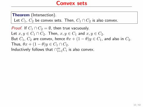
Theorem (Intersection).Let C1, C2 be convex sets. Then, C1 ∩ C2 is also convex.
Proof. If C1 ∩ C2 = ∅, then true vacuously.
Let x, y ∈ C1 ∩ C2. Then, x, y ∈ C1 and x, y ∈ C2.But C1, C2 are convex, hence θx+ (1− θ)y ∈ C1, and also in C2.Thus, θx+ (1− θ)y ∈ C1 ∩ C2.Inductively follows that ∩mi=1Ci is also convex.
12 / 42
Convex sets
Theorem (Intersection).Let C1, C2 be convex sets. Then, C1 ∩ C2 is also convex.
Proof. If C1 ∩ C2 = ∅, then true vacuously.Let x, y ∈ C1 ∩ C2. Then, x, y ∈ C1 and x, y ∈ C2.
But C1, C2 are convex, hence θx+ (1− θ)y ∈ C1, and also in C2.Thus, θx+ (1− θ)y ∈ C1 ∩ C2.Inductively follows that ∩mi=1Ci is also convex.
12 / 42
Convex sets
Theorem (Intersection).Let C1, C2 be convex sets. Then, C1 ∩ C2 is also convex.
Proof. If C1 ∩ C2 = ∅, then true vacuously.Let x, y ∈ C1 ∩ C2. Then, x, y ∈ C1 and x, y ∈ C2.But C1, C2 are convex, hence θx+ (1− θ)y ∈ C1, and also in C2.Thus, θx+ (1− θ)y ∈ C1 ∩ C2.
Inductively follows that ∩mi=1Ci is also convex.
12 / 42
Convex sets
Theorem (Intersection).Let C1, C2 be convex sets. Then, C1 ∩ C2 is also convex.
Proof. If C1 ∩ C2 = ∅, then true vacuously.Let x, y ∈ C1 ∩ C2. Then, x, y ∈ C1 and x, y ∈ C2.But C1, C2 are convex, hence θx+ (1− θ)y ∈ C1, and also in C2.Thus, θx+ (1− θ)y ∈ C1 ∩ C2.Inductively follows that ∩mi=1Ci is also convex.
12 / 42
Convex sets – more examples
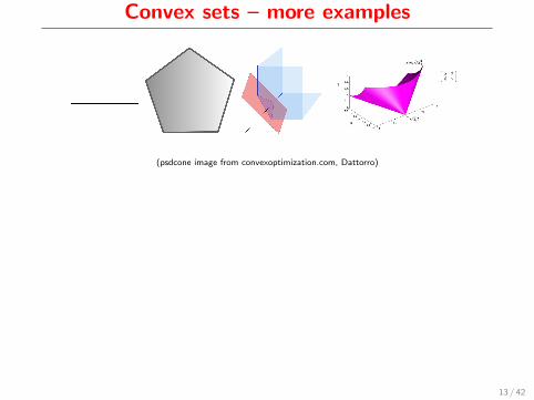
(psdcone image from convexoptimization.com, Dattorro)
13 / 42
Convex sets – more examples
♥ Let x1, x2, . . . , xm ∈ Rn. Their convex hull is
co(x1, . . . , xm) :={∑
iθixi | θi ≥ 0,
∑iθi = 1
}.
♥ Let A ∈ Rm×n, and b ∈ Rm. The set {x | Ax = b} is convex (itis an affine space over subspace of solutions of Ax = 0).
♥ halfspace{x | aTx ≤ b
}.
♥ polyhedron {x | Ax ≤ b, Cx = d}.♥ ellipsoid
{x | (x− x0)TA(x− x0) ≤ 1
}, (A: semidefinite)
♥ probability simplex {x | x ≥ 0,∑
i xi = 1}
◦
Quiz: Prove that these sets are convex.
13 / 42

Convex sets – more examples
♥ Let x1, x2, . . . , xm ∈ Rn. Their convex hull is
co(x1, . . . , xm) :={∑
iθixi | θi ≥ 0,
∑iθi = 1
}.
♥ Let A ∈ Rm×n, and b ∈ Rm. The set {x | Ax = b} is convex (itis an affine space over subspace of solutions of Ax = 0).
♥ halfspace{x | aTx ≤ b
}.
♥ polyhedron {x | Ax ≤ b, Cx = d}.
♥ ellipsoid{x | (x− x0)TA(x− x0) ≤ 1
}, (A: semidefinite)
♥ probability simplex {x | x ≥ 0,∑
i xi = 1}
◦
Quiz: Prove that these sets are convex.
13 / 42

Convex sets – more examples
♥ Let x1, x2, . . . , xm ∈ Rn. Their convex hull is
co(x1, . . . , xm) :={∑
iθixi | θi ≥ 0,
∑iθi = 1
}.
♥ Let A ∈ Rm×n, and b ∈ Rm. The set {x | Ax = b} is convex (itis an affine space over subspace of solutions of Ax = 0).
♥ halfspace{x | aTx ≤ b
}.
♥ polyhedron {x | Ax ≤ b, Cx = d}.♥ ellipsoid
{x | (x− x0)TA(x− x0) ≤ 1
}, (A: semidefinite)
♥ probability simplex {x | x ≥ 0,∑
i xi = 1}
◦
Quiz: Prove that these sets are convex.
13 / 42

Convex sets – more examples
♥ Let x1, x2, . . . , xm ∈ Rn. Their convex hull is
co(x1, . . . , xm) :={∑
iθixi | θi ≥ 0,
∑iθi = 1
}.
♥ Let A ∈ Rm×n, and b ∈ Rm. The set {x | Ax = b} is convex (itis an affine space over subspace of solutions of Ax = 0).
♥ halfspace{x | aTx ≤ b
}.
♥ polyhedron {x | Ax ≤ b, Cx = d}.♥ ellipsoid
{x | (x− x0)TA(x− x0) ≤ 1
}, (A: semidefinite)
♥ probability simplex {x | x ≥ 0,∑
i xi = 1}
◦
Quiz: Prove that these sets are convex.
13 / 42

Convex functions
14 / 42
Convex functions
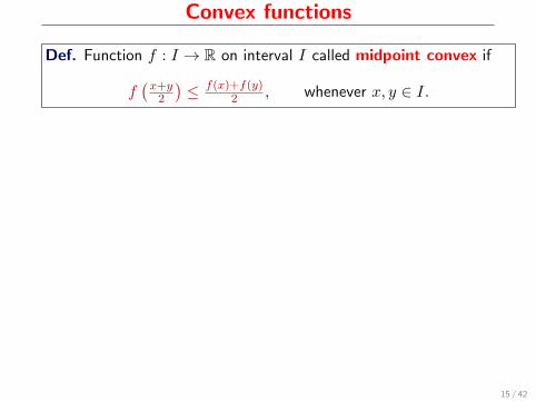
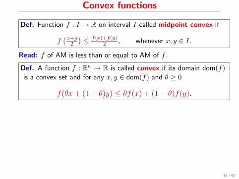
Def. Function f : I → R on interval I called midpoint convex if
f(x+y
2
)≤ f(x)+f(y)
2 , whenever x, y ∈ I.
Read: f of AM is less than or equal to AM of f .
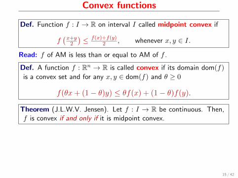
Def. A function f : Rn → R is called convex if its domain dom(f)
is a convex set and for any x, y ∈ dom(f) and θ ≥ 0
f(θx+ (1− θ)y) ≤ θf(x) + (1− θ)f(y).
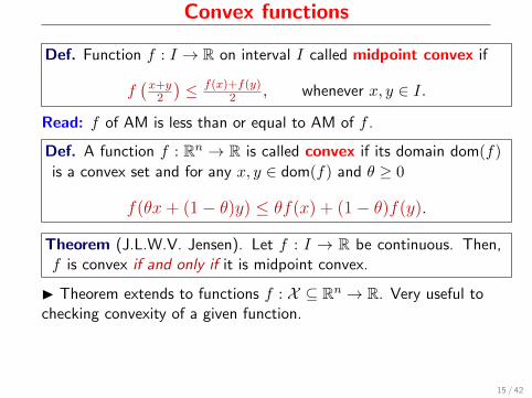
Theorem (J.L.W.V. Jensen). Let f : I → R be continuous. Then,f is convex if and only if it is midpoint convex.
I Theorem extends to functions f : X ⊆ Rn → R. Very useful tochecking convexity of a given function.
15 / 42

Convex functions
Def. Function f : I → R on interval I called midpoint convex if
f(x+y
2
)≤ f(x)+f(y)
2 , whenever x, y ∈ I.
Read: f of AM is less than or equal to AM of f .
Def. A function f : Rn → R is called convex if its domain dom(f)
is a convex set and for any x, y ∈ dom(f) and θ ≥ 0
f(θx+ (1− θ)y) ≤ θf(x) + (1− θ)f(y).
Theorem (J.L.W.V. Jensen). Let f : I → R be continuous. Then,f is convex if and only if it is midpoint convex.
I Theorem extends to functions f : X ⊆ Rn → R. Very useful tochecking convexity of a given function.
15 / 42

Convex functions
x y
f (x)
f (y)
λf (x)+ (1− λ)f (y
)
f(λx+ (1− λ)y) ≤ λf(x) + (1− λ)f(y)
16 / 42
Convex functions
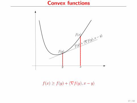
f(y)
y x
f(x)
f(y) +〈∇f(
y), x− y〉
f(x) ≥ f(y) + 〈∇f(y), x− y〉
17 / 42

Convex functions
x y
P
Q
R
z = λx+ (1− λ)y
slope PQ ≤ slope PR ≤ slope QR
18 / 42

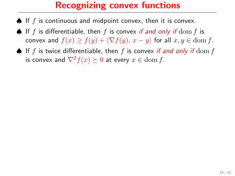
Recognizing convex functions
♠ If f is continuous and midpoint convex, then it is convex.
♠ If f is differentiable, then f is convex if and only if dom f isconvex and f(x) ≥ f(y) + 〈∇f(y), x− y〉 for all x, y ∈ dom f .
♠ If f is twice differentiable, then f is convex if and only if dom fis convex and ∇2f(x) � 0 at every x ∈ dom f .
19 / 42
Convex functions
Linear: f(θ1x+ θ2y) = θ1f(x) + θ2f(y) ; θ1, θ2 unrestricted
Concave: f(θx+ (1− θ)y) ≥ θf(x) + (1− θ)f(y)
Strictly convex: If inequality is strict for x 6= y
20 / 42
Convex functions
Example The pointwise maximum of a family of convex functions isconvex. That is, if f(x; y) is a convex function of x for every y insome “index set” Y, then
f(x) := maxy∈Y
f(x; y)
is a convex function of x (set Y is arbitrary).
Example Let f : Rn → R be convex. Let A ∈ Rm×n, and b ∈ Rm.Prove that g(x) = f(Ax+ b) is convex.
Exercise: Verify truth of above examples.
21 / 42
Convex functions
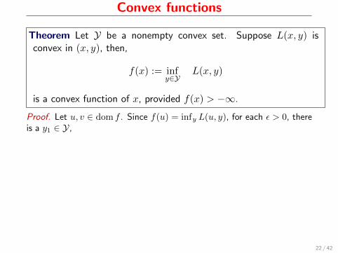
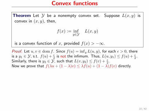
Theorem Let Y be a nonempty convex set. Suppose L(x, y) isconvex in (x, y), then,
f(x) := infy∈Y
L(x, y)
is a convex function of x, provided f(x) > −∞.
Proof. Let u, v ∈ dom f . Since f(u) = infy L(u, y), for each ε > 0, thereis a y1 ∈ Y, s.t. f(u) + ε
2 is not the infimum. Thus, L(u, y1) ≤ f(u) + ε2 .
Similarly, there is y2 ∈ Y, such that L(v, y2) ≤ f(v) + ε2 .
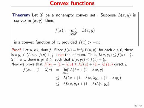
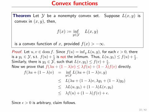
Now we prove that f(λu+ (1− λ)v) ≤ λf(u) + (1− λ)f(v) directly.
f(λu+ (1− λ)v) = infy∈Y
L(λu+ (1− λ)v, y)
≤ L(λu+ (1− λ)v, λy1 + (1− λ)y2)
≤ λL(u, y1) + (1− λ)L(v, y2)
≤ λf(u) + (1− λ)f(v) + ε.
Since ε > 0 is arbitrary, claim follows.
22 / 42

Convex functions
Theorem Let Y be a nonempty convex set. Suppose L(x, y) isconvex in (x, y), then,
f(x) := infy∈Y
L(x, y)
is a convex function of x, provided f(x) > −∞.
Proof. Let u, v ∈ dom f .
Since f(u) = infy L(u, y), for each ε > 0, thereis a y1 ∈ Y, s.t. f(u) + ε
2 is not the infimum. Thus, L(u, y1) ≤ f(u) + ε2 .
Similarly, there is y2 ∈ Y, such that L(v, y2) ≤ f(v) + ε2 .
Now we prove that f(λu+ (1− λ)v) ≤ λf(u) + (1− λ)f(v) directly.
f(λu+ (1− λ)v) = infy∈Y
L(λu+ (1− λ)v, y)
≤ L(λu+ (1− λ)v, λy1 + (1− λ)y2)
≤ λL(u, y1) + (1− λ)L(v, y2)
≤ λf(u) + (1− λ)f(v) + ε.
Since ε > 0 is arbitrary, claim follows.
22 / 42
Convex functions
Theorem Let Y be a nonempty convex set. Suppose L(x, y) isconvex in (x, y), then,
f(x) := infy∈Y
L(x, y)
is a convex function of x, provided f(x) > −∞.
Proof. Let u, v ∈ dom f . Since f(u) = infy L(u, y), for each ε > 0, thereis a y1 ∈ Y,
s.t. f(u) + ε2 is not the infimum. Thus, L(u, y1) ≤ f(u) + ε
2 .Similarly, there is y2 ∈ Y, such that L(v, y2) ≤ f(v) + ε
2 .Now we prove that f(λu+ (1− λ)v) ≤ λf(u) + (1− λ)f(v) directly.
f(λu+ (1− λ)v) = infy∈Y
L(λu+ (1− λ)v, y)
≤ L(λu+ (1− λ)v, λy1 + (1− λ)y2)
≤ λL(u, y1) + (1− λ)L(v, y2)
≤ λf(u) + (1− λ)f(v) + ε.
Since ε > 0 is arbitrary, claim follows.
22 / 42

Convex functions
Theorem Let Y be a nonempty convex set. Suppose L(x, y) isconvex in (x, y), then,
f(x) := infy∈Y
L(x, y)
is a convex function of x, provided f(x) > −∞.
Proof. Let u, v ∈ dom f . Since f(u) = infy L(u, y), for each ε > 0, thereis a y1 ∈ Y, s.t. f(u) + ε
2 is not the infimum. Thus, L(u, y1) ≤ f(u) + ε2 .
Similarly, there is y2 ∈ Y, such that L(v, y2) ≤ f(v) + ε2 .
Now we prove that f(λu+ (1− λ)v) ≤ λf(u) + (1− λ)f(v) directly.
f(λu+ (1− λ)v) = infy∈Y
L(λu+ (1− λ)v, y)
≤ L(λu+ (1− λ)v, λy1 + (1− λ)y2)
≤ λL(u, y1) + (1− λ)L(v, y2)
≤ λf(u) + (1− λ)f(v) + ε.
Since ε > 0 is arbitrary, claim follows.
22 / 42
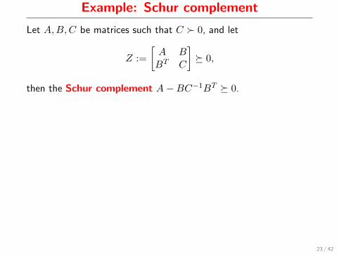
Example: Schur complement
Let A,B,C be matrices such that C � 0, and let
Z :=
[A BBT C
]� 0,
then the Schur complement A−BC−1BT � 0.
Proof. L(x, y) = [x, y]TZ[x, y] is convex in (x, y) since Z � 0
Observe that f(x) = infy L(x, y) = xT (A−BC−1BT )x is convex.
(We skipped ahead and solved ∇yL(x, y) = 0 to minimize).
23 / 42

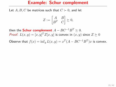
Example: Schur complement
Let A,B,C be matrices such that C � 0, and let
Z :=
[A BBT C
]� 0,
then the Schur complement A−BC−1BT � 0.Proof. L(x, y) = [x, y]TZ[x, y] is convex in (x, y) since Z � 0
Observe that f(x) = infy L(x, y) = xT (A−BC−1BT )x is convex.
(We skipped ahead and solved ∇yL(x, y) = 0 to minimize).
23 / 42
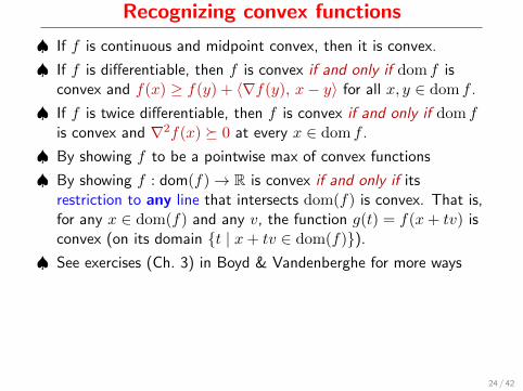
Recognizing convex functions
♠ If f is continuous and midpoint convex, then it is convex.
♠ If f is differentiable, then f is convex if and only if dom f isconvex and f(x) ≥ f(y) + 〈∇f(y), x− y〉 for all x, y ∈ dom f .
♠ If f is twice differentiable, then f is convex if and only if dom fis convex and ∇2f(x) � 0 at every x ∈ dom f .
♠ By showing f to be a pointwise max of convex functions
♠ By showing f : dom(f)→ R is convex if and only if itsrestriction to any line that intersects dom(f) is convex. That is,for any x ∈ dom(f) and any v, the function g(t) = f(x+ tv) isconvex (on its domain {t | x+ tv ∈ dom(f)}).
♠ See exercises (Ch. 3) in Boyd & Vandenberghe for more ways
24 / 42

Operations preservingconvexity
25 / 42

Operations preserving convexity
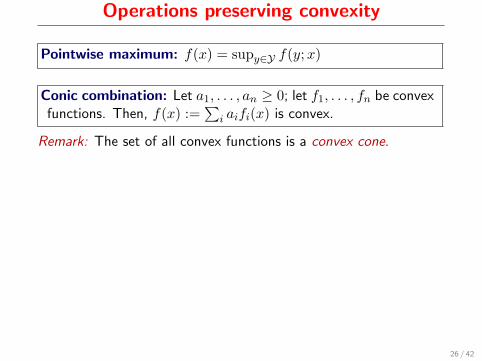
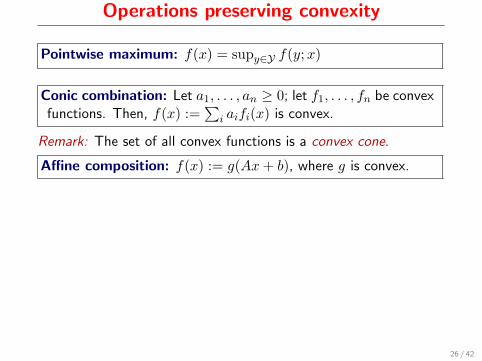
Pointwise maximum: f(x) = supy∈Y f(y;x)
Conic combination: Let a1, . . . , an ≥ 0; let f1, . . . , fn be convexfunctions. Then, f(x) :=
∑i aifi(x) is convex.
Remark: The set of all convex functions is a convex cone.
Affine composition: f(x) := g(Ax+ b), where g is convex.
26 / 42

Operations preserving convexity
Pointwise maximum: f(x) = supy∈Y f(y;x)
Conic combination: Let a1, . . . , an ≥ 0; let f1, . . . , fn be convexfunctions. Then, f(x) :=
∑i aifi(x) is convex.
Remark: The set of all convex functions is a convex cone.
Affine composition: f(x) := g(Ax+ b), where g is convex.
26 / 42
Operations preserving convexity
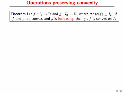
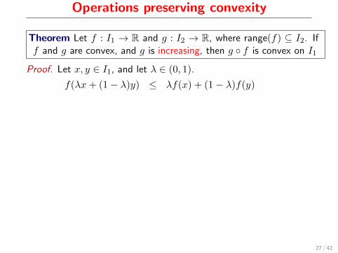
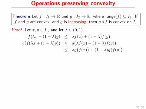
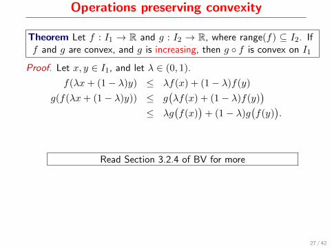
Theorem Let f : I1 → R and g : I2 → R, where range(f) ⊆ I2. Iff and g are convex, and g is increasing, then g ◦ f is convex on I1
Proof. Let x, y ∈ I1, and let λ ∈ (0, 1).
f(λx+ (1− λ)y) ≤ λf(x) + (1− λ)f(y)
g(f(λx+ (1− λ)y)) ≤ g(λf(x) + (1− λ)f(y)
)≤ λg
(f(x)
)+ (1− λ)g
(f(y)
).
Read Section 3.2.4 of BV for more
27 / 42

Operations preserving convexity
Theorem Let f : I1 → R and g : I2 → R, where range(f) ⊆ I2. Iff and g are convex, and g is increasing, then g ◦ f is convex on I1
Proof. Let x, y ∈ I1, and let λ ∈ (0, 1).
f(λx+ (1− λ)y) ≤ λf(x) + (1− λ)f(y)
g(f(λx+ (1− λ)y)) ≤ g(λf(x) + (1− λ)f(y)
)≤ λg
(f(x)
)+ (1− λ)g
(f(y)
).
Read Section 3.2.4 of BV for more
27 / 42

Operations preserving convexity
Theorem Let f : I1 → R and g : I2 → R, where range(f) ⊆ I2. Iff and g are convex, and g is increasing, then g ◦ f is convex on I1
Proof. Let x, y ∈ I1, and let λ ∈ (0, 1).
f(λx+ (1− λ)y) ≤ λf(x) + (1− λ)f(y)
g(f(λx+ (1− λ)y)) ≤ g(λf(x) + (1− λ)f(y)
)
≤ λg(f(x)
)+ (1− λ)g
(f(y)
).
Read Section 3.2.4 of BV for more
27 / 42
Operations preserving convexity
Theorem Let f : I1 → R and g : I2 → R, where range(f) ⊆ I2. Iff and g are convex, and g is increasing, then g ◦ f is convex on I1
Proof. Let x, y ∈ I1, and let λ ∈ (0, 1).
f(λx+ (1− λ)y) ≤ λf(x) + (1− λ)f(y)
g(f(λx+ (1− λ)y)) ≤ g(λf(x) + (1− λ)f(y)
)≤ λg
(f(x)
)+ (1− λ)g
(f(y)
).
Read Section 3.2.4 of BV for more
27 / 42
Examples
28 / 42

Quadratic
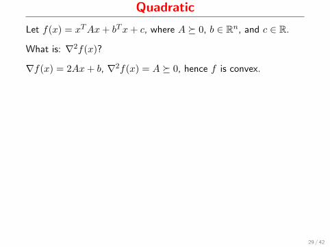
Let f(x) = xTAx+ bTx+ c, where A � 0, b ∈ Rn, and c ∈ R.
What is: ∇2f(x)?
∇f(x) = 2Ax+ b, ∇2f(x) = A � 0, hence f is convex.
29 / 42

Quadratic
Let f(x) = xTAx+ bTx+ c, where A � 0, b ∈ Rn, and c ∈ R.
What is: ∇2f(x)?
∇f(x) = 2Ax+ b, ∇2f(x) = A � 0, hence f is convex.
29 / 42
Quadratic
Let f(x) = xTAx+ bTx+ c, where A � 0, b ∈ Rn, and c ∈ R.
What is: ∇2f(x)?
∇f(x) = 2Ax+ b, ∇2f(x) = A � 0, hence f is convex.
29 / 42

Indicator
Let IX be the indicator function for X defined as:
IX (x) :=
{0 if x ∈ X ,∞ otherwise.
Note: IX (x) is convex if and only if X is convex.
30 / 42
Indicator
Let IX be the indicator function for X defined as:
IX (x) :=
{0 if x ∈ X ,∞ otherwise.
Note: IX (x) is convex if and only if X is convex.
30 / 42
Distance to a set
Example Let Y be a convex set. Let x ∈ Rn be some point. Thedistance of x to the set Y is defined as
dist(x,Y) := infy∈Y
‖x− y‖.
Because ‖x− y‖ is jointly convex in (x, y), the function dist(x,Y)is a convex function of x.
31 / 42

Norms
Let f : Rn → R be a function that satisfies
1 f(x) ≥ 0, and f(x) = 0 if and only if x = 0 (definiteness)
2 f(λx) = |λ|f(x) for any λ ∈ R (positive homogeneity)
3 f(x+ y) ≤ f(x) + f(y) (subadditivity)
Such a function is called a norm. We usually denote norms by ‖x‖.
Theorem Norms are convex.
Proof. Immediate from subadditivity and positive homogeneity.
32 / 42

Norms
Let f : Rn → R be a function that satisfies
1 f(x) ≥ 0, and f(x) = 0 if and only if x = 0 (definiteness)
2 f(λx) = |λ|f(x) for any λ ∈ R (positive homogeneity)
3 f(x+ y) ≤ f(x) + f(y) (subadditivity)
Such a function is called a norm. We usually denote norms by ‖x‖.Theorem Norms are convex.
Proof. Immediate from subadditivity and positive homogeneity.
32 / 42

Vector norms
Example (`2-norm): Let x ∈ Rn. The Euclidean or `2-norm is
‖x‖2 =(∑
i x2i
)1/2
Example (`p-norm): Let p ≥ 1. ‖x‖p =(∑
i |xi|p)1/p
Exercise: Verify that ‖x‖p is indeed a norm.
Example (`∞-norm): ‖x‖∞ = max1≤i≤n |xi|
Example (Frobenius-norm): Let A ∈ Rm×n. The Frobenius norm
of A is ‖A‖F :=√∑
ij |aij |2; that is, ‖A‖F =√
Tr(A∗A).
33 / 42

Vector norms
Example (`2-norm): Let x ∈ Rn. The Euclidean or `2-norm is
‖x‖2 =(∑
i x2i
)1/2Example (`p-norm): Let p ≥ 1. ‖x‖p =
(∑i |xi|p
)1/pExercise: Verify that ‖x‖p is indeed a norm.
Example (`∞-norm): ‖x‖∞ = max1≤i≤n |xi|
Example (Frobenius-norm): Let A ∈ Rm×n. The Frobenius norm
of A is ‖A‖F :=√∑
ij |aij |2; that is, ‖A‖F =√
Tr(A∗A).
33 / 42

Mixed norms
Def. Let x ∈ Rn1+n2+···+nG be a vector partitioned into subvectorsxj ∈ Rnj , 1 ≤ j ≤ G. Let p := (p0, p1, p2, . . . , pG), where pj ≥ 1.Consider the vector ξ := (‖x1‖p1 , · · · , ‖xG‖pG). Then, we definethe mixed-norm of x as
‖x‖p := ‖ξ‖p0 .
Example `1,q-norm: Let x be as above.
‖x‖1,q :=∑G
i=1‖xi‖q.
This norm is popular in machine learning, statistics.
34 / 42

Matrix Norms
Induced norm
Let A ∈ Rm×n, and let ‖·‖ be any vector norm. We define aninduced matrix norm as
‖A‖ := sup‖x‖6=0
‖Ax‖‖x‖ .
Verify that above definition yields a norm.
I Clearly, ‖A‖ = 0 iff A = 0 (definiteness)
I ‖αA‖ = |α| ‖A‖ (homogeneity)
I ‖A+B‖ = sup ‖(A+B)x‖‖x‖ ≤ sup ‖Ax‖+‖Bx‖
‖x‖ ≤ ‖A‖ + ‖B‖.
35 / 42
Operator norm
Example Let A be any matrix. Then, the operator norm of A is
‖A‖2 := sup‖x‖2 6=0
‖Ax‖2‖x‖2
.
‖A‖2 = σmax(A), where σmax is the largest singular value of A.
• Warning! Generally, largest eigenvalue of a matrix is not a norm!
• ‖A‖1 and ‖A‖∞—max-abs-column and max-abs-row sums.
• ‖A‖p generally NP-Hard to compute for p 6∈ {1, 2,∞}• Schatten p-norm: `p-norm of vector of singular value.
• Exercise: Let σ1 ≥ σ2 ≥ · · · ≥ σn ≥ 0 be singular values of amatrix A ∈ Rm×n. Prove that
‖A‖(k) :=∑k
i=1σi(A),
is a norm; 1 ≤ k ≤ n.
36 / 42

Operator norm
Example Let A be any matrix. Then, the operator norm of A is
‖A‖2 := sup‖x‖2 6=0
‖Ax‖2‖x‖2
.
‖A‖2 = σmax(A), where σmax is the largest singular value of A.
• Warning! Generally, largest eigenvalue of a matrix is not a norm!
• ‖A‖1 and ‖A‖∞—max-abs-column and max-abs-row sums.
• ‖A‖p generally NP-Hard to compute for p 6∈ {1, 2,∞}
• Schatten p-norm: `p-norm of vector of singular value.
• Exercise: Let σ1 ≥ σ2 ≥ · · · ≥ σn ≥ 0 be singular values of amatrix A ∈ Rm×n. Prove that
‖A‖(k) :=∑k
i=1σi(A),
is a norm; 1 ≤ k ≤ n.
36 / 42

Operator norm
Example Let A be any matrix. Then, the operator norm of A is
‖A‖2 := sup‖x‖2 6=0
‖Ax‖2‖x‖2
.
‖A‖2 = σmax(A), where σmax is the largest singular value of A.
• Warning! Generally, largest eigenvalue of a matrix is not a norm!
• ‖A‖1 and ‖A‖∞—max-abs-column and max-abs-row sums.
• ‖A‖p generally NP-Hard to compute for p 6∈ {1, 2,∞}• Schatten p-norm: `p-norm of vector of singular value.
• Exercise: Let σ1 ≥ σ2 ≥ · · · ≥ σn ≥ 0 be singular values of amatrix A ∈ Rm×n. Prove that
‖A‖(k) :=∑k
i=1σi(A),
is a norm; 1 ≤ k ≤ n.
36 / 42

Operator norm
Example Let A be any matrix. Then, the operator norm of A is
‖A‖2 := sup‖x‖2 6=0
‖Ax‖2‖x‖2
.
‖A‖2 = σmax(A), where σmax is the largest singular value of A.
• Warning! Generally, largest eigenvalue of a matrix is not a norm!
• ‖A‖1 and ‖A‖∞—max-abs-column and max-abs-row sums.
• ‖A‖p generally NP-Hard to compute for p 6∈ {1, 2,∞}• Schatten p-norm: `p-norm of vector of singular value.
• Exercise: Let σ1 ≥ σ2 ≥ · · · ≥ σn ≥ 0 be singular values of amatrix A ∈ Rm×n. Prove that
‖A‖(k) :=∑k
i=1σi(A),
is a norm; 1 ≤ k ≤ n.
36 / 42
Dual norms
Def. Let ‖·‖ be a norm on Rn. Its dual norm is
‖u‖∗ := sup{uTx | ‖x‖ ≤ 1
}.
Exercise: Verify that ‖u‖∗ is a norm.
Exercise: Let 1/p+ 1/q = 1, where p, q ≥ 1. Show that ‖·‖q isdual to ‖·‖p. In particular, the `2-norm is self-dual.
37 / 42
Dual norms
Def. Let ‖·‖ be a norm on Rn. Its dual norm is
‖u‖∗ := sup{uTx | ‖x‖ ≤ 1
}.
Exercise: Verify that ‖u‖∗ is a norm.
Exercise: Let 1/p+ 1/q = 1, where p, q ≥ 1. Show that ‖·‖q isdual to ‖·‖p. In particular, the `2-norm is self-dual.
37 / 42

Fenchel Conjugate
38 / 42

Fenchel conjugate
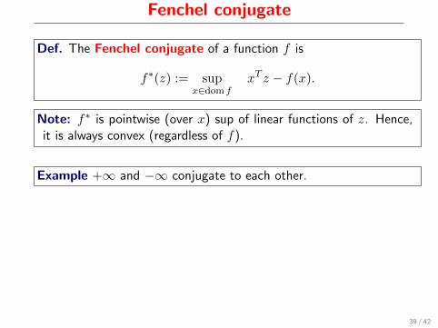
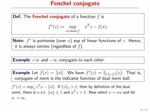
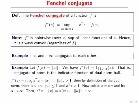
Def. The Fenchel conjugate of a function f is
f∗(z) := supx∈dom f
xT z − f(x).
Note: f∗ is pointwise (over x) sup of linear functions of z. Hence,it is always convex (regardless of f).
Example +∞ and −∞ conjugate to each other.
Example Let f(x) = ‖x‖. We have f∗(z) = I‖·‖∗≤1(z). That is,conjugate of norm is the indicator function of dual norm ball.
f∗(z) = supx zTx− ‖x‖. If ‖z‖∗ > 1, then by definition of the dual
norm, there is u s.t. ‖u‖ ≤ 1 and uT z > 1. Now select x = αu and let
α→∞. Then, zTx− ‖x‖ = α(zTu− ‖u‖)→∞. If ‖z‖∗ ≤ 1, then
zTx ≤ ‖x‖‖z‖∗, which implies the sup must be zero.
39 / 42
Fenchel conjugate
Def. The Fenchel conjugate of a function f is
f∗(z) := supx∈dom f
xT z − f(x).
Note: f∗ is pointwise (over x) sup of linear functions of z. Hence,it is always convex (regardless of f).
Example +∞ and −∞ conjugate to each other.
Example Let f(x) = ‖x‖. We have f∗(z) = I‖·‖∗≤1(z). That is,conjugate of norm is the indicator function of dual norm ball.
f∗(z) = supx zTx− ‖x‖. If ‖z‖∗ > 1, then by definition of the dual
norm, there is u s.t. ‖u‖ ≤ 1 and uT z > 1. Now select x = αu and let
α→∞. Then, zTx− ‖x‖ = α(zTu− ‖u‖)→∞. If ‖z‖∗ ≤ 1, then
zTx ≤ ‖x‖‖z‖∗, which implies the sup must be zero.
39 / 42

Fenchel conjugate
Def. The Fenchel conjugate of a function f is
f∗(z) := supx∈dom f
xT z − f(x).
Note: f∗ is pointwise (over x) sup of linear functions of z. Hence,it is always convex (regardless of f).
Example +∞ and −∞ conjugate to each other.
Example Let f(x) = ‖x‖. We have f∗(z) = I‖·‖∗≤1(z). That is,conjugate of norm is the indicator function of dual norm ball.
f∗(z) = supx zTx− ‖x‖. If ‖z‖∗ > 1, then by definition of the dual
norm, there is u s.t. ‖u‖ ≤ 1 and uT z > 1.
Now select x = αu and let
α→∞. Then, zTx− ‖x‖ = α(zTu− ‖u‖)→∞. If ‖z‖∗ ≤ 1, then
zTx ≤ ‖x‖‖z‖∗, which implies the sup must be zero.
39 / 42
Fenchel conjugate
Def. The Fenchel conjugate of a function f is
f∗(z) := supx∈dom f
xT z − f(x).
Note: f∗ is pointwise (over x) sup of linear functions of z. Hence,it is always convex (regardless of f).
Example +∞ and −∞ conjugate to each other.
Example Let f(x) = ‖x‖. We have f∗(z) = I‖·‖∗≤1(z). That is,conjugate of norm is the indicator function of dual norm ball.
f∗(z) = supx zTx− ‖x‖. If ‖z‖∗ > 1, then by definition of the dual
norm, there is u s.t. ‖u‖ ≤ 1 and uT z > 1. Now select x = αu and let
α→∞.
Then, zTx− ‖x‖ = α(zTu− ‖u‖)→∞. If ‖z‖∗ ≤ 1, then
zTx ≤ ‖x‖‖z‖∗, which implies the sup must be zero.
39 / 42
Fenchel conjugate
Def. The Fenchel conjugate of a function f is
f∗(z) := supx∈dom f
xT z − f(x).
Note: f∗ is pointwise (over x) sup of linear functions of z. Hence,it is always convex (regardless of f).
Example +∞ and −∞ conjugate to each other.
Example Let f(x) = ‖x‖. We have f∗(z) = I‖·‖∗≤1(z). That is,conjugate of norm is the indicator function of dual norm ball.
f∗(z) = supx zTx− ‖x‖. If ‖z‖∗ > 1, then by definition of the dual
norm, there is u s.t. ‖u‖ ≤ 1 and uT z > 1. Now select x = αu and let
α→∞. Then, zTx− ‖x‖ = α(zTu− ‖u‖)→∞.
If ‖z‖∗ ≤ 1, then
zTx ≤ ‖x‖‖z‖∗, which implies the sup must be zero.
39 / 42

Fenchel conjugate
Def. The Fenchel conjugate of a function f is
f∗(z) := supx∈dom f
xT z − f(x).
Note: f∗ is pointwise (over x) sup of linear functions of z. Hence,it is always convex (regardless of f).
Example +∞ and −∞ conjugate to each other.
Example Let f(x) = ‖x‖. We have f∗(z) = I‖·‖∗≤1(z). That is,conjugate of norm is the indicator function of dual norm ball.
f∗(z) = supx zTx− ‖x‖. If ‖z‖∗ > 1, then by definition of the dual
norm, there is u s.t. ‖u‖ ≤ 1 and uT z > 1. Now select x = αu and let
α→∞. Then, zTx− ‖x‖ = α(zTu− ‖u‖)→∞. If ‖z‖∗ ≤ 1, then
zTx ≤ ‖x‖‖z‖∗, which implies the sup must be zero.
39 / 42

Fenchel conjugate
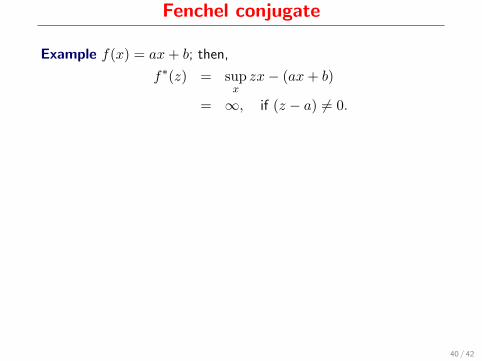
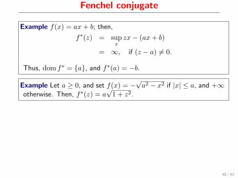
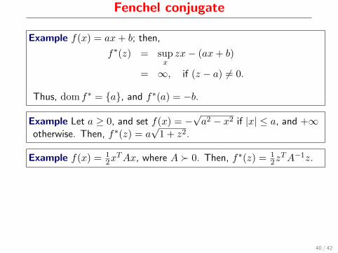
Example f(x) = ax+ b; then,
f∗(z) = supxzx− (ax+ b)
= ∞, if (z − a) 6= 0.
Thus, dom f∗ = {a}, and f∗(a) = −b.
Example Let a ≥ 0, and set f(x) = −√a2 − x2 if |x| ≤ a, and +∞
otherwise. Then, f∗(z) = a√
1 + z2.
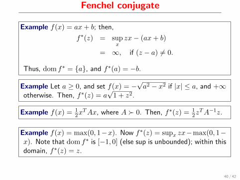
Example f(x) = 12x
TAx, where A � 0. Then, f∗(z) = 12z
TA−1z.
Example f(x) = max(0, 1−x). Now f∗(z) = supx zx−max(0, 1−x). Note that dom f∗ is [−1, 0] (else sup is unbounded); within thisdomain, f∗(z) = z.
40 / 42
Fenchel conjugate
Example f(x) = ax+ b; then,
f∗(z) = supxzx− (ax+ b)
= ∞, if (z − a) 6= 0.
Thus, dom f∗ = {a}, and f∗(a) = −b.
Example Let a ≥ 0, and set f(x) = −√a2 − x2 if |x| ≤ a, and +∞
otherwise. Then, f∗(z) = a√
1 + z2.
Example f(x) = 12x
TAx, where A � 0. Then, f∗(z) = 12z
TA−1z.
Example f(x) = max(0, 1−x). Now f∗(z) = supx zx−max(0, 1−x). Note that dom f∗ is [−1, 0] (else sup is unbounded); within thisdomain, f∗(z) = z.
40 / 42

Misc Convexity
41 / 42
Other forms of convexity
♣ Log-convex: log f is convex; log-cvx =⇒ cvx;
♣ Log-concavity: log f concave; not closed under addition!
♣ Exponentially convex: [f(xi + xj)] � 0, for x1, . . . , xn
♣ Operator convex: f(λX + (1− λ)Y ) � λf(X) + (1− λ)f(Y )
♣ Quasiconvex: f(λx+ (1− λy)) ≤ max {f(x), f(y)}♣ Pseudoconvex: 〈∇f(y), x− y〉 ≥ 0 =⇒ f(x) ≥ f(y)
♣ Discrete convexity: f : Zn → Z; “convexity + matroid theory.”
42 / 42
Other forms of convexity
♣ Log-convex: log f is convex; log-cvx =⇒ cvx;
♣ Log-concavity: log f concave; not closed under addition!
♣ Exponentially convex: [f(xi + xj)] � 0, for x1, . . . , xn
♣ Operator convex: f(λX + (1− λ)Y ) � λf(X) + (1− λ)f(Y )
♣ Quasiconvex: f(λx+ (1− λy)) ≤ max {f(x), f(y)}
♣ Pseudoconvex: 〈∇f(y), x− y〉 ≥ 0 =⇒ f(x) ≥ f(y)
♣ Discrete convexity: f : Zn → Z; “convexity + matroid theory.”
42 / 42

Other forms of convexity
♣ Log-convex: log f is convex; log-cvx =⇒ cvx;
♣ Log-concavity: log f concave; not closed under addition!
♣ Exponentially convex: [f(xi + xj)] � 0, for x1, . . . , xn
♣ Operator convex: f(λX + (1− λ)Y ) � λf(X) + (1− λ)f(Y )
♣ Quasiconvex: f(λx+ (1− λy)) ≤ max {f(x), f(y)}♣ Pseudoconvex: 〈∇f(y), x− y〉 ≥ 0 =⇒ f(x) ≥ f(y)
♣ Discrete convexity: f : Zn → Z; “convexity + matroid theory.”
42 / 42
Other forms of convexity
♣ Log-convex: log f is convex; log-cvx =⇒ cvx;
♣ Log-concavity: log f concave; not closed under addition!
♣ Exponentially convex: [f(xi + xj)] � 0, for x1, . . . , xn
♣ Operator convex: f(λX + (1− λ)Y ) � λf(X) + (1− λ)f(Y )
♣ Quasiconvex: f(λx+ (1− λy)) ≤ max {f(x), f(y)}♣ Pseudoconvex: 〈∇f(y), x− y〉 ≥ 0 =⇒ f(x) ≥ f(y)
♣ Discrete convexity: f : Zn → Z; “convexity + matroid theory.”
42 / 42
Recommended