IEEE
Proo
f
IEEE TRANSACTIONS ON BIOMEDICAL ENGINEERING, VOL. 00, NO. 00, 2012 1
Consciousness and Depth of Anesthesia AssessmentBased on Bayesian Analysis of EEG Signals
1
2
Tai Nguyen-Ky∗, Member, IEEE, Peng (Paul) Wen, and Yan Li, Member, IEEE3
Abstract—This study applies Bayesian techniques to analyze4EEG signals for the assessment of the consciousness and depth of5anesthesia (DoA). This method takes the limiting large-sample nor-6mal distribution as posterior inferences to implement the Bayesian7paradigm. The maximum a posterior (MAP) is applied to denoise8the wavelet coefficients based on a shrinkage function. When the9anesthesia states change from awake to light, moderate, and deep10anesthesia, the MAP values increase gradually. Based on these11changes, a new function BDoA is designed to assess the DoA. The12new proposed method is evaluated using anesthetized EEG record-13ings and BIS data from 25 patients. The Bland–Alman plot is used14to verify the agreement of BDoA and the popular BIS index. A15correlation between BDoA and BIS was measured using predic-16tion probability PK . In order to estimate the accuracy of DoA,17the effect of sample n and variance τ on the maximum posterior18probability is studied. The results show that the new index accu-19rately estimates the patient’s hypnotic states. Compared with the20BIS index in some cases, the BDoA index can estimate the patient’s21hypnotic state in the case of poor signal quality.22
Index Terms—Bayesian, depth of anesthesia (DoA), electroen-23cephalogram (EEG), maximum a posterior (MAP), maximum24posterior probability (MPP), wavelet transform.25
I. INTRODUCTION26
ANESTHETISTS seek an early warning of a patient’s level27
of hypnosis in real time. A number of methods have been28
developed over the years to detect the level of consciousness29
and determine the depth of anesthesia (DoA), such as clinical30
signs (systolic blood pressure, heart rate, sweating, and tears),31
spontaneous surface electromyogram, heart rate variability, the32
minimum alveolar concentration, lower esophageal contractility33
(LOC), and isolated forearm technique (IFT). However, these34
methods are not reliable and could not achieve the desired accu-35
racy of anesthetic depth, as individual patients have variability36
and various factors, such as the degree of stimulation, pain in-37
duced by surgery and the use of concomitant analgesic drugs. It38
Manuscript received June 13, 2012; revised November 5, 2012 andDecember 19, 2012; accepted December 20, 2012. Date of publication; dateof current version. This work was supported in part by the Toowoomba HospitalFoundation, Australia. Asterisk indicates corresponding author.
∗T. Nguyen-Ky is with the Faculty of Engineering and Surveying, Centre forSystems Biology, University of Southern Queensland, Toowoomba, Qld., 4350,Australia (e-mail: [email protected]).
P. Wen is with the Faculty of Engineering and Surveying, Centre for SystemsBiology, University of Southern Queensland, Toowoomba, Qld., 4350, Australia(e-mail: [email protected]).
Y. Li is with the Department of Mathematics and Computing, Centre forSystems Biology, University of Southern Queensland, Toowoomba, Qld., 4350,Australia (e-mail: [email protected]).
Digital Object Identifier 10.1109/TBME.2012.2236649
is impossible to gain a constant level of consciousness through 39
precalculating the exact dose of anesthetics. Clinical investiga- 40
tions and individual cases report that some patients had been 41
aware during the anesthesia at times when there were no ab- 42
normalities in blood pressure and heart rate [1]. LOC was not 43
reliable for detecting of inadequate anesthesia when the primary 44
anesthetic agent was used [2]. In the IFT method, patients were 45
asked to move their fingers to check the level of the DoA. How- 46
ever, some patients could hear the commands but were unable 47
to move the isolated arm. The incidence of movement with IFT 48
could vary with the choice of anesthetic [3], [4]. 49
Results from both human and animal studies demonstrate that 50
changes in electroencephalogram (EEG) with anesthesia pri- 51
marily reflect hypnotic information [5]–[8]. Several DoA moni- 52
toring devices were developed based on EEG. Currently, the BIS 53
monitor is widely used in hospitals. Although the algorithms of 54
these monitors are different and are not fully published, their 55
basic principles can be described as the following. The cere- 56
bral state index is calculated using a fuzzy logic combination of 57
four subparameters of the EEG signals in the time domain and 58
the frequency domain [9]. The patient state index is the result 59
of a complex computation that combines weighted quantitative 60
EEG parameters reflecting many dimensions of brain electrical 61
activities [10]. Entropy index monitoring is based on the acqui- 62
sition and processing of raw EEG and FEMG signals by using 63
Entropy algorithms to produce two parameters: state entropy 64
over the frequency range of 0.8–32 Hz, and response entropy 65
over the frequency range of 0.8–47 Hz [11]. In the Nacotrend 66
index, numerous quantitative features were extracted from the 67
time and the frequency domains, such as spectral parameters, 68
entropy measures, and autoregressive parameters [12]. The BIS 69
index is calculated from the following four parameters: 1) burst 70
suppression ratio (BSR); 2) quazi suppression index; 3) relative 71
β ratio; and 4) synchfastslow [13]. 72
These monitors are widely used in clinical practice and they 73
work satisfactorily most of the time. However, there are still 74
some criticisms in some special cases, such as not consistent 75
with the clinical observations [14], [15], not adequately de- 76
tecting the transition between consciousness and unconscious- 77
ness [16], and not responsive to some anesthetic agents [17]. The 78
time-domain analysis is used for the detection of epochs that rep- 79
resent the electrical suppression of EEG signals. However, that 80
only happens in the case of very deep anesthesia. Therefore, 81
these analyses could not be used for the light anesthesia state 82
detection. 83
There are other developed methods for monitoring the DoA, 84
such as wavelet transformation [18] and modified detrended 85
moving average [19]. Recently, an adaptive time–frequency 86
0018-9294/$31.00 © 2012 IEEE

IEEE
Proo
f
2 IEEE TRANSACTIONS ON BIOMEDICAL ENGINEERING, VOL. 00, NO. 00, 2012
analysis method based on ensemble empirical-model decom-87
position was used to analyze EEG signals for estimating the88
DoA [20]. The spectral features of EEG signals were proposed89
in [21] for separating the anesthetic effects. The Isomap-based90
estimation was used to assess neurophysiological changes dur-91
ing anesthesia [22]. The Hurst exponent and the wavelet trans-92
form was applied in multiscale rescaled range analysis algo-93
rithms to measure the anesthetic drug effects on brain activ-94
ity [23].95
The Bayesian method was also applied to analyze the EEG96
signals for the DoA [24], [25]. Rezek et al. presented an autore-97
gressive class of polyspectral models in the variation Bayesian98
framework [24]. Their results showed that the estimated higher99
order spectra can give a significant improvement for the DoA.100
The midlatency auditory evoked potentials were used to estimate101
the DoA by a neural network and the Bayesian rule [25].102
In this paper, a statistical method is developed to estimate the103
DoA based on the Bayesian method. A denoising raw EEG data104
technique is introduced using the maximum a posterior (MAP)105
to compute a new Bayesian-wavelet threshold for the large sam-106
ple posterior distribution. After denoising, the maximum pos-107
terior probability (MPP) is used to study the distribution of the108
EEG signal. A new function BDoA is designed to estimate the109
anesthesia levels. To the best of our knowledge, this is the first110
time a Bayesian method is proposed for assessing the DoA based111
on the EEG signal.112
This paper is organized as follows. In Section II, the data ac-113
quisition and a Bayesian wavelet denoising method is presented114
with a new threshold Tn . Section III introduces a relationship115
between the maximum posterior and anesthesia states. A new116
function BDoA for monitoring the DoA is proposed in this sec-117
tion. The Bland–Altman method is used to test the degree of118
agreement between the new index BDoA and the BIS method in119
Section IV. The experiment results are provided in Section V.120
The discussion and the limitations of the study are presented in121
Section VI. Finally, a short conclusion is drawn in Section VII.122
II. BAYESIAN WAVELET DENOISING123
A. Data Acquisition124
Based on the relevant ethics approvals, the EEG data were125
collected at the Toowoomba St. Vincent’s Hospital. The formal126
consents were obtained from 25 adult patients (ASA I or II, age127
42–76 years, weight 64–130 kg, gender 10 F/15 M). Opera-128
tion types include minor orthopedics, peripheral generals, si-129
nus, thyroid, middle ear, abdominals, chest wall, laparoscopic130
abdos, open abdos, lower abdos, perineal surgery, and laparo-131
scopic bowels. Typical drug administration included earlier132
pharmaceuticals intravenous midazolam 0.05 mg/kg, fentanyl133
1.5–3 μg/kg, or alfentanil 15–30 μg/kg. Intravenous propofol134
was induction 1–3 mg/kg as clinically appropriate and mainte-135
nance with inhaled sevoflurane or desflurane in oxygen-enriched136
air, or in 60% nitrous oxide in air. The airway was supported137
by endotracheal intubation or by laryngeal mask airway as138
indicated clinically. The timing of all intravenous dosing and139
significant intraoperative events as indicated by the BIS mon-140
itor clock was recorded by the attending anesthetist. In the141
meantime, clinical observations by the attending anesthetists 142
during the data collection were also recorded for the 143
comparison. 144
The BIS Quatro sensor was attached to the patient’s forehead. 145
Raw EEG data, BIS values, EMG, and signal quantity index 146
(SQI) were obtained and exported to a USB drive. Raw EEG 147
data were presented as a binary file documenting two channels 148
of unfiltered signals. Each EEG sample was a 16-bit signed 149
integer in units of 0.05 μV. The data were sampled at 128 times 150
per second for each channel. Q1151
B. Denoised Method 152
A noise EEG signal yi of size n can be presented as 153
yi = xi + ε, i = 1, 2, ..., n (1)
where xi is the true EEG signal and ε represents a noise which is 154
the sequence of independent and identically distributed random 155
variable. In the wavelet domain, a transform of yi has the form 156
of 157
d = d + ε (2)
where d = Wy; d = Wx; ε = Wε; y = y1 , ..., yn ;x = x1 , ..., 158
xn ; and ε = ε1 , ..., εn . 159
Here, W is an orthogonal matrix, d is a noisy wavelet coef- 160
ficient, d is the true coefficient, and ε is noise. Our goal is to 161
estimate d from the noise observation d. The supposition to test 162
is H0 : d = 0 versus H1 : d �= 0. 163
A Bayesian wavelet threshold was proposed in [29]–[31]. 164
Prior information with Bayesian estimation techniques was ap- 165
plied for the wavelet-based denoising. The MAP was used to es- 166
timate d from the noisy observation d. A large sample posterior 167
distribution and approximations were presented by Press in [32]. 168
The limiting large-sample normal distribution was adopted for 169
posterior inferences of implementing the Bayesian paradigm. 170
In [33], a larger posterior mode for the wavelet threshold was 171
proposed by Cutillo et al. based on the MAP with the threshold 172
T = 2σ√
2k − 1, k > 1/2. (3)
C. Statistic Model 173
For the model, the assumption is made that the wavelet coef- 174
ficient d is normally distributed with the parameters μ and σ2 , 175
and its density function p(d|μ, σ2) is given by 176
p(d|μ, σ2) =1
σ√
2πexp
{− 1
2σ2 (d − μ)2}
. (4)
If d ∼ N(μ, σ2), then E(d) = μ and V (d) = σ2 . The param- 177
eter μ of the normal distribution is determined by the expected 178
value and the parameter σ2 by the variance of the random vari- 179
able d. 180
Suppose we have normal observations d|d ∼ N(d, σ2), 181
where σ is known and the prior distribution for d is 182
d|λ2 ∼ N(μ, λ2), λ2 ∼ (λ2)−nk , k > 0 (5)
where λ2 is the single unknown hyperparameter. Here, it is 183
assumed that the parameters d are independent and identi- 184

IEEE
Proo
f
NGUYEN-KY et al.: CONSCIOUSNESS AND DEPTH OF ANESTHESIA ASSESSMENT BASED ON BAYESIAN ANALYSIS OF EEG SIGNALS 3
cally distributed, and conditional on other parameters, such as185
d ∼ N(μ, λ2). Consider a conjugate prior to p(d|d) and p(d|λ2),186
the hierarchical Bayes induces the following structure [32]:187
λ2 ∼ p(λ2), d|λ2 ∼ p(d|λ2), d|d ∼ p(d|d). (6)
The likelihood function l(d|d) is the probability of observing188
d being conditional on the values of d. The prior distribution on189
d [33] is190
p(d) =∫
p(d|λ2)p(λ2)d(λ2). (7)
The posterior distribution expresses the information of d191
based on both the sample data and the prior information [33]192
p(d, d) =∫
p(d|d)p(d|λ2)p(λ2)d(λ2). (8)
D. New Bayesian Wavelet Threshold193
The MAP estimator developed for the Gaussian case is194
p(d, d) ∝ p(d, d) ∝ l(d). (9)
Here, l(d) is the likelihood [33]195
l(d) = e−1
2 σ 2 (d−d)2(d − μ)2( 1
2 −nk). (10)
The goal here is to find the parameters d that maximize the196
posterior probability. The logarithm of the posterior is propor-197
tional to198
log{
p(d, d)}∝ log
{l(d)
}= L(d)
={− 1
2σ2 (d − d)2}
+ (1 − 2nk) log(d − μ
). (11)
Maximum posterior estimators are asymptotically equivalent199
to the classical maximum likelihood estimators. The eventual200
models of the posterior p(d|d) happen when L(d) maximizes.201
The derivative of L(d) with respect to d is202
∂L(d)
∂d=
d2 − (μ + d)d + μd + σ2(2nk − 1)σ2(μ − d)
. (12)
Setting the derivative equal to 0, we obtain203
d ≥ μ + 2√
σ2(2nk − 1). (13)
To estimate the noise variance σ2 from the noisy wavelet204
coefficients, the finest scale wavelet coefficient a1 is used to205
compute a median estimator in [26]–[28] as206
σ2 =median(|a1 |)
0.6745. (14)
Combining (13) and (14), a new threshold Tn is defined as207
Tn = log(μ + 2
√σ2(2nk − 1)
)(15)
with208
μ = mean(x). (16)
The BDoA function is used to compare the efficiency of two209
denoising thresholds which were presented in (3) and (15). The210
detail of BDoA will be presented in the next section (see (24)).211
Fig. 1. Comparison between the two denoising thresholds: (a) BDoA trendusing the threshold in (3). (b) BDoA trend using the new proposed Bayesianthreshold in (15).
In Fig. 1(b), BDoA clearly shows the changes of patient’s states 212
from awake state to deep anesthesia, and from general anesthe- 213
sia to awake. This BDoA trend used the new proposed Bayesian 214
threshold in (25). In contrast, the trend of BDoA which used 215
the threshold in (3) has some spike noise during general anes- 216
thesia period as shown in Fig. 1(a). This indicates that our new 217
Bayesian threshold is better than the threshold in (3) for denois- 218
ing raw EEG signals. 219
III. BAYESIAN METHOD FOR THE DOA 220
In this section, we derive the estimate method for monitoring 221
the DoA using a Bayesian method. If the EEG signal is presented 222
by x and denotes the set of unknown parameters by θ, the 223
likelihood function f(x|θ) is the probability of observing the 224
data x being conditional on the values of parameter θ. The prior 225
distribution for θ is π(θ). Bayesian’s theorem gives the posterior 226
probability density function (pdf) for parameter θ as 227
f(θ|x) =f(x|θ)π(θ)∫f(x|θ)π(θ)dθ
(17)
where f denotes the joint pdf of the data and π denotes the prior 228
pdf of θ. If f is replaced by the likelihood function L(θ|x), we 229
have 230
f(θ|x) =L(x|θ)π(θ)∫L(x|θ)π(θ)dθ
. (18)
Suppose the EEG signal x has the normal observation x|θ ∼ 231
N(θ, σ2), where sigma is known and the prior distribution for 232
θ is θ ∼ N(μ, τ 2). We have 233
E(θ|x) = μ +τ 2
σ2 + τ 2 (x − μ) =σ2μ + τ 2x
σ2 + τ 2 (19)
Var(θ|x) =τ 2σ2
σ2 + τ 2 . (20)
The posterior for θ is the normal pdf as 234
yθ = f(θ|μ, σ) =1
σ√
2πe−
( θ −μ ) 2
2 σ 2 . (21)

IEEE
Proo
f
4 IEEE TRANSACTIONS ON BIOMEDICAL ENGINEERING, VOL. 00, NO. 00, 2012
Fig. 2. Posterior, likelihood, and prior density function of the EEG signal withpatient 19.
Fig. 3. Comparison between the maximum of different posterior distributions,corresponding to different anesthesia states in four sample ranges.
Fig. 2 shows the posterior, prior, and likelihood of patient’s235
EEG data in the case of normal distributions. The posterior,236
likelihood and, prior density functions are shown together for237
the unknown parameter θ in this figure. The posterior and like-238
lihood density functions are considerably more concentrated239
around their maximum values than the prior density function. A240
posterior density function is used to characterize the values of241
the parameters for the EEG data.242
A. MPP of the θ Distribution243
Let MPP be the maximum value of the posterior of yθ , to give244
MPP = max(yθ ). (22)
MPP will be used to estimate the DoA. Fig. 3(a) shows four245
posterior graphs of yθ in different states of anesthesia. The max-246
imum values of the posterior in Fig. 3(a) have changed from low247
TABLE IRELATION BETWEEN THE ANESTHESIA STATES AND THE MPP FOR A PATIENT
values to high values when the BIS trend of patient 19 changed 248
from awake to the deep anesthesia states in Fig. 3(b). Patient 19 249
was a 74 yr old, 100 kg male. BIS values were recorded between 250
09:21:36 am and 10:33:44 am. Anesthesia induction was with 251
intravenous midazolam 3 mg at 09:22:00, alfentanil 1000 μg at 252
09:22:03, and propofol 120 mg at 09:25:53. At 09:25:55, inhaled 253
sevoflurane and nitrous oxide were introduced. The rectangles 254
1, 2, 3, and 4 in Fig. 3(a) cover the posteriors 1, 2, 3, and 4 255
which are corresponding to the ranges 1, 2, 3, and 4 in Fig. 3(b). 256
Range 1 indicates the awake state with the BIS values from 80 257
to 97. Range 2 shows the moderate anesthesia state with the BIS 258
values from 41 to 43. Range 3 represents the light anesthesia 259
state with the BIS values from 59 to 68; while range 4 is the 260
deep anesthesia state with the BIS values from 25 to 26. 261
Table I presents a relationship between the anesthesia states 262
and the MPP. When the anesthesia states change from awake 263
to light, moderate, and deep anesthesia, the MPP values in- 264
crease from 0.0954, 0.1065, 0.1083, and 0.1316, respectively. 265
These changes are also shown in Fig. 3, corresponding to the 266
four ranges in the four rectangles. These rectangles are used to 267
connect the BIS trend and the posterior distribution in different 268
ranges. The ranges for computing the MPP in Fig. 3 are selected, 269
based on the levels of the anesthesia states. Each individual pos- 270
terior distribution is computed within its own range and then 271
compared on the same axis. The BIS trend shows the changes 272
of anesthesia states over time. 273
B. Monitor the DoA 274
The MPP values have different scales for individual patients. 275
Therefore, their values are converted to a common scale through 276
normalization. A new scale for the MPP in the range of [0, 1] is 277
MPP = MPP/max(MPP). Fig. 4 presents a scatter plot of the BIS 278
and the MPP for 25 patients. The BIS values are on the x-axis 279
in the range of [0, −100] and the MPP values are on the y-axis 280
in the range of [0, −1]. A least-squares curve-fitting method is 281
used to find the straight line by minimizing the distance from 282
each point to this line. The line equation we obtained is 283
MPP = −0.0077BIS + 0.87. (23)
284
This line is the best fit to a set of data points for minimizing 285
the sum of the squared distances between the line and the data 286
points. Based on the relation of the MPP values and the BIS 287
values in (32) when anesthesia states change from awake to 288
deep anesthesia, a new function is proposed to estimate the 289

IEEE
Proo
f
NGUYEN-KY et al.: CONSCIOUSNESS AND DEPTH OF ANESTHESIA ASSESSMENT BASED ON BAYESIAN ANALYSIS OF EEG SIGNALS 5
Fig. 4. Scatter plot and regression line of the BIS and MPP for 25 patients.
Fig. 5. Scatter plot, histograms, and regression line for the BDoA and BISvalues.
anesthesia levels as290
BDoA = (1 − MPP) × 100 + VOFFSET . (24)
Fig. 5 presents a scatter plot of the BDoA and the BIS val-291
ues, and their histograms on the horizontal and vertical axes.292
The r-squared values r2 = 0.9285 and r = 0.93 show a strong293
correlation between the BDoA and the BIS. The statistical sig-294
nificance was assumed at probability levels of p < 0.005.295
IV. AGREEMENT OF THE BDOA AND THE BIS296
To evaluate and compare our proposed method with other297
established methods, such as the BIS, the Bland–Altman method298
[36] is used to test the degree of the agreement between the299
proposed and BIS methods.300
Defining the difference of the BDoA and the BIS index as301
(BDoA–BIS), the mean difference is dff = mean(BDoA–BIS),302
and the standard deviation of the differences is SD = std(BDoA–303
BIS). If the differences are normally distributed, 95% of the304
differences lie between (dff –2SD) and (dff – 2SD). The calcu-305
lation of the 95% limits of agreement is based on the assumption306
Fig. 6. Distribution of the differences (BDoA –BIS) and the normal fitting.
Fig. 7. Bland–Altman plot shows the difference (BDoA –BIS) versus the av-erage of values measured with 95% limits of agreement.
that the differences are normally distributed. The distribution of 307
the differences can be checked by drawing a normal plot or 308
histogram. 309
Fig. 6 presents the fitting of the normal distribution of 310
the differences (BDoA—BIS). In this figure, the distribution 311
of the differences matches well with the normal fitting. The 312
Bland–Altman plot is presented in Fig. 7. The Bland–Altman 313
method calculates the mean difference between two methods 314
of the measurement (the “bias”) and 95% limits of agreement 315
as the mean difference (2SD). The Bland–Altman can include 316
an estimation of confidence intervals for the bias and limits 317
of agreement. In Fig. 7, there is a bias of 0.3379. The upper 318
limit of agreement is (dff + 2SD) = 16.1, and the lower limit 319
is (dff – 2SD) = –11.28. The 94.73% (17.500/18.473) limit 320
of agreement presents a visual judgment of how well the two 321
methods of the measurements agree. 322
Prediction probability PK was assessed as described by Smith 323
et al. [37] as a statistical test to assess the capability of a classifier 324
to discern different levels of anesthesia. In this study, PK is 325
calculated using the PK tool 1.2 by Denis et al. [38]. A value of 326

IEEE
Proo
f
6 IEEE TRANSACTIONS ON BIOMEDICAL ENGINEERING, VOL. 00, NO. 00, 2012
Fig. 8. EEG histogram is fitted to the different probability densities: normal,gamma, Rayleigh, extreme, inverse Gaussian, and exponential.
PK = 0.5 means that the index predicts the observed state no327
better than 50/50 chance, and a value of PK = 1.0 means that the328
index always predicts the observed state correctly. A value of329
p < 0.05 was considered significant. PK was calculated for each330
patient. An average of these PK (mean(PK ) = 0.807) preserves331
a good correlation between expected index values BDoA and332
BIS.333
V. EXPERIMENT RESULTS334
A. Probability Distribution of the EEG Signal335
Assuming that the EEG data are the observations from a con-336
tinuous probability distribution, to model the behavior of those337
data, the modeling will then begin by studying the distribution338
of the data. In practice, it is difficult to know exactly the prob-339
ability distribution of the observations. A simple approach to340
model the behavior of the data is to form a histogram of the341
data. Fig. 8 plots the histogram of the EEG signal in the data342
vector using a number of bin bars in the histograms. The EEG343
histograms are fitted to the different probability densities, such344
as normal, gamma, Rayleigh, extreme, inverse Gaussian, and345
exponential. As shown in Fig. 8(a), the normal probability den-346
sity model matches the histograms well. Therefore, the normal347
pdf is used to compute the pdf of the EEG signal.348
B. Parameter Estimation349
If the hyperparameters (μ and τ) are known, the posterior350
distribution for θ can be obtained as351
θ|x ∼ N
(σ2μ + τ 2x
σ2 + τ 2 ,τ 2σ2
σ2 + τ 2
). (25)
In practice, the situation parameters n and τ vary over time352
with different patients. Therefore, the BDoA function may not353
be accurate for the large samples of patients. In order to estimate354
the accuracy of DoA, the effect of parameters n and τ on the355
MPP is studied with different values. With sample n and the356
sample mean X = 1/n∑n
i=1 xi , to give357
θ|x1 , x2 , . . . , xn ∼ N(μp, σp) (26)
Fig. 9. Impacts of n and τ values on the posterior values. (a) MAP valuesincrease when the sample n increases. (b) MAP values decrease when thevariance τ increases.
TABLE IIBDoA VALUES IN AWAKE STATE WITH DIFFERENT SAMPLES (n)
AND VARIANCE τ VALUES, BIS = 80–100
with 358
μp =σ2μ + nτ 2X
σ2 + nτ 2 , σp =τ 2σ2
σ2 + nτ 2 . (27)
The impacts of the value of n and τ on the posterior values are 359
shown in Fig. 9. In Fig. 9(a), when n has the values of 100, 1000, 360
and 10000, the posteriors get the maximum values as 0.0074, 361
0.2263, and 0.6737, respectively. The MAP value will have a 362
high value with a large sample n and vice versa. In Fig. 9(b), 363
when τ has the values of 5, 10, 20, and 40, the posteriors get 364
the maximum values as 0.1072, 0.0820, 0.0744, and 0.0724, 365
respectively. 366
C. BDoA Estimation Based on Bayesian Parameters 367
In this section, BDoA values are considered based on the 368
change of the different samples (n) and variance τ values. Four 369
states of anesthesia are studied such as awake, light anesthesia, 370
moderate anesthesia, and deep anesthesia states, corresponding 371
to the BIS value ranges at 80–100, 60–80, 40–60, and 20–40, 372
respectively. The simulation results are presented in Tables II– 373
V. The samples (n) are chosen with the values as n = 128 × k, 374
with k = 1, 5, 10, 15, 20, 30. The variance τ are chosen with 375
IEEE
Proo
f
NGUYEN-KY et al.: CONSCIOUSNESS AND DEPTH OF ANESTHESIA ASSESSMENT BASED ON BAYESIAN ANALYSIS OF EEG SIGNALS 7
TABLE IIIBDoA VALUES IN LIGHT ANESTHESIA STATE WITH DIFFERENT SAMPLES (n)
AND VARIANCE τ VALUES, BIS = 70–80
TABLE IVBDoA VALUES IN MODERATE ANESTHESIA STATE WITH DIFFERENT SAMPLES
(n) AND VARIANCE τ VALUES, BIS = 40–55
the values as τ = 5 × m, with m = 1, 2, . . ., 10. In Table II, in376
awake state, the BDoA values are in the range of 80–100, except377
the change of n and τ values. However, in Tables III and IV,378
the BDoA values are only correct with the situations when the379
values n are 128 × k, 128 × k, and 128 × k, with k = 20, 25,380
and 30. Finally, in Table V, the BDoA values are correct with381
the situations when the values of k are 20 and 25. Summarizing382
for different cases of anesthesia states, the sample n is chosen383
in the range of [2560, 3200], and τ values can vary from 5 to384
50.385
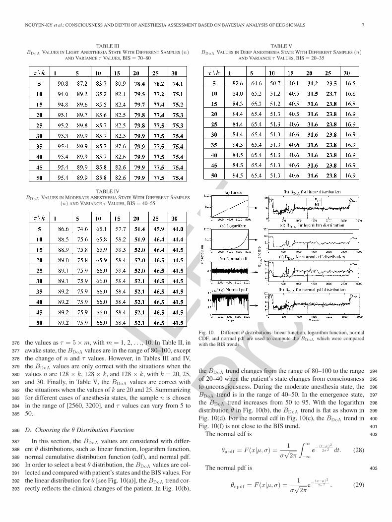
D. Choosing the θ Distribution Function386
In this section, the BDoA values are considered with differ-387
ent θ distributions, such as linear function, logarithm function,388
normal cumulative distribution function (cdf), and normal pdf.389
In order to select a best θ distribution, the BDoA values are col-390
lected and compared with patient’s states and the BIS values. For391
the linear distribution for θ [see Fig. 10(a)], the BDoA trend cor-392
rectly reflects the clinical changes of the patient. In Fig. 10(b),393
TABLE VBDoA VALUES IN DEEP ANESTHESIA STATE WITH DIFFERENT SAMPLES (n)
AND VARIANCE τ VALUES, BIS = 20–35
Fig. 10. Different θ distributions: linear function, logarithm function, normalCDF, and normal pdf are used to compute the BDoA which were comparedwith the BIS trends.
the BDoA trend changes from the range of 80–100 to the range 394
of 20–40 when the patient’s state changes from consciousness 395
to unconsciousness. During the moderate anesthesia state, the 396
BDoA trend is in the range of 40–50. In the emergence state, 397
the BDoA trend increases from 50 to 95. With the logarithm 398
distribution θ in Fig. 10(b), the BDoA trend is flat as shown in 399
Fig. 10(d). For the normal cdf in Fig. 10(c), the BDoA trend in 400
Fig. 10(f) is not close to the BIS trend. 401
The normal cdf is 402
θncdf = F (x|μ, σ) =1
σ√
2π
∫ ∞
−∞e−
( t−μ ) 2
2 σ 2 dt. (28)
The normal pdf is 403
θnpdf = F (x|μ, σ) =1
σ√
2πe−
(x −μ ) 2
2 σ 2 . (29)

IEEE
Proo
f
8 IEEE TRANSACTIONS ON BIOMEDICAL ENGINEERING, VOL. 00, NO. 00, 2012
Fig. 11. Burst suppression happens from 390 to 397 s. (a) Comparison betweenBDoA and BIS trends. BDoA index can show the DoA values during the burstsuppression time. (b) Sample EEG signal during the burst suppression time.
For the normal pdf distribution of θ in Fig. 10(g), the BDoA404
trend in Fig. 10(h) shows the same result as the BDoA trend in405
Fig. 10(b). In both cases, the BDoA trends are close to the BIS406
trends. Therefore, the linear function and the normal pdf can be407
chosen for the θ distribution.408
E. Burst Suppression EEG Pattern409
During the deep anesthesia, the EEG voltage may change410
from high activity to low or even isoelectricity. This pattern is411
known as burst suppression. The BSR is a time-domain EEG412
parameter developed to quantify this phenomenon (i.e., a flat413
EEG or no significant electrical activity in the brain). The burst414
suppression is recognized as those periods longer than 0.50 s,415
during which the EEG voltage does not exceed approximately416
±5.0 μV [6]. The BDoA and BIS trends are shown in Fig. 11(a).417
This figure shows the BDoA values in the range of 13.3–15.5 sec-418
onds during burst suppression, lasted 4 s from 390 to 394 s. The419
EEG signal during the burst suppression is shown in Fig. 11(b).420
During this period, the EEG signal has an amplitude value lower421
than 5.0 μV.422
F. Patient’s State in the Case of Poor Signal Quality423
The BIS index is a good monitor but in some cases BIS424
index could not display the values on the screen when signal425
quality indicator (SQI) was lower than 15. This paper claims426
that BDoA can display the DoA values in the case of poor signal427
quality but the BIS could not. For these cases, the BIS monitor428
displays a notice “Excessive artifact detected in signal”. In the429
recorded BIS data of excel file, the value –3276.8 was labeled430
in these cases. In the BIS monitor, the signal quality indicator431
(SQI) is a measure of the signal quality for the EEG channel432
source and is calculated based on impedance data, artifacts, and433
other variables. When the signal quality is too low to accurately434
calculate a BIS value, the affected BIS value and other trends435
will not be displayed on the screen. Potential artifacts may be436
caused by poor skin contact (high impedance), muscle activity or437
rigidity, head and body motion, sustained eye movements, etc.438
Only “valid” BIS values are displayed on the monitor screen439
when signal quality index (SQI) is above 15 [22].440
Fig. 12. DoA values in the case of poor signal quality of Patient 12: a com-parison between the BDoA and BIS trends. From 0 to 180 s, when SQI is lowerthan 15, the BDoA values can display the DoA values but the BIS cannot.
Fig. 13. During general anesthesia, the BDoA values can display the DoAvalues but the BIS cannot when SQI is lower than 15.
Fig. 12 shows a case of poor signal quality of Patient 12 441
when patient’s state changed from awake to anesthesia. Patient 442
12 was a 63 yr old, 72 kg, female. Surgery was undertaken from 443
10:31:33 am to 10:52:26 am. Drug administration consisted 444
of midazolam (4 mg) as a sedative drug at 10:31:35 am. At 445
10:31:55 am, alfentanil (1000 μg) was used as strong pain relief 446
given only once during the operation. Parecoxib (40 mg) and 447
Propofol (160 mg) were used at 10:32:55 am and 10:33:30 448
am, respectively. At 10:33:35 am, desflurane and nitrous oxide 449
(N2O) were started. From 0 to 180 s (10:31:33 am to 10:34:33 450
am), the BIS cannot display the DoA values. The clinically 451
important transition from the awake state (BIS = 100) to deep 452
anesthesia (BIS = 33.6) is masked by this phenomenon (see 453
Fig. 12). In this case, the anesthetist could not use the BIS index 454
to estimate the state of the patient. 455
Another case of poor signal quality is presented in Fig. 13 dur- 456
ing general anesthesia. However, the proposed BDoA index can 457
compute and display the DoA index at times when SQI is lower 458
than 15 and the invalid BIS value did not display on the moni- 459
tor screen. The proposed BDoA displays are shown in Figs. 12 460
and 13. Compared with the BIS index in these cases, during the 461
periods of poor signal quality, the results of this Bayesian MMP 462
method better correlate with clinical observations. Those other 463
cases can be found when BIS values dropped as shown in Figs. 464
14 and 16(c). 465

IEEE
Proo
f
NGUYEN-KY et al.: CONSCIOUSNESS AND DEPTH OF ANESTHESIA ASSESSMENT BASED ON BAYESIAN ANALYSIS OF EEG SIGNALS 9
Fig. 14. Comparison between the BDoA and BIS trends in the case of poorsignal quality in Patient 11.
Fig. 15. Comparison between the BDoA and BIS trends in the case of poorsignal quality in Patient 19.
There is a case where BDOA goes wrong while BIS seems466
to be reliable as shown in Fig. 15. At the awake state, BDoA467
drops two times to value 25 when BIS only drops one time. At468
the second 1500, the BIS value increases but BDOA decreases469
at the recovery time. In this case, probably there are impedance-470
related artifacts that can arise from electrode drift on the skin. In471
the other cases during general anesthetic, dropped BDoA values472
do not happen but the BIS does.473
G. Testing Denoise Algorithm474
In order to check the denoise result, the BDoA function is475
used for three parameters y, x, and ε in (1): y = x + ε. Here,476
y is a noise EEG signal, x is the EEG signal after denoising,477
and ε is a noise. Fig. 16(a), (b), and (c) shows the BDoA of478
the raw EEG signal, noise, and the EEG signal after denoising,479
respectively. BDoA(y) and BDoA(ε) trends are in the range of480
96.5–100 and do not have any relation to the patient’s states. In481
contrast, BDoA(x) trend is close to the BIS trend. This means482
that the denoising algorithm did not filter out any important483
information regarding the DoA.484
VI. DISCUSSION485
In this paper, clinically observed changes in conscious state486
were also observed and recorded by the attending anesthetist487
Fig. 16. (a) BDoA (y): BDoA of raw EEG signal, (b) BDoA (ε): BDoA ofnoise, and (c) BDoA (x): BDoA of EEG signal after denoising in Patient 4.
for comparison. The patients’ responses were the overall (ex- 488
perienced) clinical impressions which took into account patient 489
movement, lacrimation, heart rate, blood pressure, respiratory 490
effort, pupil status, and, importantly, what surgery the patient 491
had undergone. The two main components to create the anes- 492
thetic state are hypnosis created with drugs, and analgesia cre- 493
ated with the nitrous oxide. The earlier pharmaceuticals mida- 494
zolam 4 mg and alfentanil 1000 μg were induced. Most patients 495
might not remember but might well move in response to stimuli 496
after these drugs have been given. Loss of consciousness (LOC) 497
occurs reliably at about 30–60 s after intravenous propofol. As- 498
sessment of LOC clinically was by lack of response to verbal 499
and tactile stimuli. Loss of the lash reflex was used in the case 500
of doubt. However, we did not have the plasmatic concentra- 501
tions of sedative drugs. This could be a limitation of this study, 502
especially with a small number of patients. Data exported to 503
a USB drive and transferred to a portable computer for offline 504
analysis. The results were compared with the BIS in the simu- 505
lation, the same as with real-time analysis. Therefore, extensive 506
testing with a larger set of subjects in real time is necessary 507
to further improve the method. Furthermore, clinical anesthe- 508
sia scales, such as the observer’s assessment of anesthesia and 509
sedation and drug concentrations, can be used as an additional 510
reference to improve the accuracy of the DoA estimation. 511
VII. CONCLUSION 512
This paper studies a Bayesian method for denoising EEG sig- 513
nals and estimating the hypnotic DoA. First, an adaptive thresh- 514
old for Bayesian wavelet denoising is proposed. The wavelet 515
transform coefficients are modeled with prior probability distri- 516
butions. A Bayesian technique is used to denoise the coefficients 517
based on this prior information and the likelihood function. A 518
new Bayesian threshold Tn is better than the threshold in [33] 519
for denoising raw EEG signals. 520

IEEE
Proo
f
10 IEEE TRANSACTIONS ON BIOMEDICAL ENGINEERING, VOL. 00, NO. 00, 2012
Second, a new index BDoA is proposed based on the MPP521
values. When the anesthesia states change from awake to light,522
moderate, and deep anesthesia, the MPP values increase corre-523
spondingly. The Bland–Altman method is used to test the degree524
of agreement between our proposed method and the BIS index.525
The scatterplot indicates the agreement rates of 94.73% between526
BDoA and BIS indices. The result mean (PK ) = 0.807 preserves527
a good correlation between the expected index values BDoA and528
BIS.529
In order to estimate the accuracy of DoA, the effect of sample530
n and variance τ on MPP is studied. The MPP value will have531
the high value with a large sample n and vice versa. For different532
anesthesia states, the sample n is chosen in the range of [2560,533
3200], and τ value can vary from 5 to 50. In order to select the534
best θ distributions, the BDoA values are collected and compared535
with the patient’s states and the BIS values. In the cases of the536
linear function and the normal pdf, the BDoA trends are close to537
the BIS trends. Therefore, these functions are chosen for the θ538
distribution.539
The simulation results show that the new index accurately540
estimates patient’s hypnotic states. In addition, BDoA can reflect541
the clinical observations better than the BIS index during the542
periods of poor signal quality.543
ACKNOWLEDGMENT544
The authors would like to express their appreciation to545
Dr. R. Gray, a senior anesthetist at Toowoomba Base Hospital546
and St. Vincent’s Hospital, Australia, for his clinical knowl-547
edge and expertise in anesthesia. They would also like to thank548
Dr. D. Jordan and his team for supporting the PK tool 1.2.549
REFERENCES550
[1] N. Moerman, B. Bonke, and J. Oosting, “Awareness and recall during551general anesthesia: Facts and feelings,” Anesthesiology, vol. 79, no. 3,552pp. 454–464, 1993.553
[2] I. M. Schwieger, C. C. Hug, R. I. Hall, and F. S. Zlam, “Is lower554esophageal contractility a reliable indicator of the adequacy of opioid555anesthesia?,” J. Clin. Monit. Comput., vol. 5, no. 3, pp. 164–169, 1988.556
[3] I. F. Russell, “Comparison of wakefulness with two anaesthetic regimens:557Total IV balanced anaesthesia,” Brit. J. Anaesth., vol. 58, pp. 965–968,5581986.559
Q2 [4] I. F. Russell, “Auditory perception under anaesthesia,” Anaesthesia,560vol. 34, p. 211, 1979.561
[5] G. M. Terri, V. Saini, and B. C. Weldon, “Anesthetic management and562one-year mortality after noncardiac surgery,” Anesth. Analgesia, vol. 100,563no. 1, pp. 4–10, 2005.564
[6] I. J. Rampil, “A primer for EEG signal processing in anesthesia,” Anes-565thesiology, vol. 89, no. 4, pp. 980–1002, 1998.566
Q3 [7] J. D. Andrew, G. H. Huang, C. Czarnecki et al., “Awareness during567anesthesia in children: A prospective cohort study,” Anaesth. Analgesia,568vol. 100, no. 3, pp. 653–661, 2005.569
[8] M. Agarwal and R. Griffiths, “Monitoring the depth of anaesthesia,”570Anaesth. Intensive Care Med., vol. 5, no. 10, pp. 343–344, 2004.571
[9] E. W. Jensen. (2005). “Cerebral state monitoring and pharmacodynamic572modelling by advanced fuzzy inference—State of the art,” [Online]. Avail-573able: http://www.amca2005.unibe.ch574
[10] D. Drover and H. R. Ortega, “Patient state index,” Best Practice Res. Clin.575Anaes., vol. 20, no. 1, pp. 121–128, 2006.576
[11] H. Viertio-Oja, V. Maja, and M. Sarkela, “Description of the entropyTM577algorithm as applied in the datex-ohmeda s/5TM entropy module,” Acta578Anaesth. Scand., vol. 48, no. 2, pp. 154–161, 2004.579
[12] S. Kreuer and W. Wilhelm, “The narcotrend monitor,” Best Practice Res.580Clin. Anaesth., vol. 20, no. 1, pp. 111–119, 2006.581
[13] C. J. D. Pomfrett and A. J. Pearson, “EEG monitoring using bispectral 582analysis,” Eng. Sci. Edu. J., vol. 7, no. 4, pp. 155–157, 1998. 583
[14] R. E. Anderson, G. Barr, H. Assareh et al., “Cerebral state index dur- 584ing anaesthetic induction: A comparative study with propofol or nitrous 585oxide,” Acta Anaesth. Scand., vol. 49, no. 6, pp. 750–753, 2005. 586
[15] R. E. Anderson and J. G. Jakobsson, “Cerebral state index response to 587incision: A clinical study in day-surgical patients,” Acta Anaesth. Scand., 588vol. 50, no. 6, pp. 749–753, 2006. 589
[16] G. Schneider, E. F. Kochs, B. Horn et al., “Narcotrend(r) does not ad- 590equately detect the transition between awareness and unconsciousness 591in surgical patients,” Anesthesiology, vol. 101, no. 5, pp. 1105–1111, 5922004. 593
[17] G. Schneider, S. Schoniger, E. Kochs et al., “Does bispectral analysis add 594anything but complexity? BIS sub-components may be superior to BIS 595for detection of awareness,” Brit. J. Anaesth., vol. 93, no. 4, pp. 596–597, 5962004. 597
[18] T. Nguyen-Ky, P. P. Wen, Y. Li, and R. Gray, “Measuring and reflecting 598depth of anaesthesia in real-time for general anaesthesia patients,” IEEE 599Trans. Inf. Technol. Biomed., vol. 15, no. 2, pp. 630–639, Jul. 2011. 600
[19] T. Nguyen-Ky, P. P. Wen, and Yan Li, “An improved de-trended moving 601average method for accurately monitoring the depth of anaesthesia,” IEEE 602Trans. Biomed. Eng., vol. 57, no. 10, pp. 2369–2378, Oct. 2010. 603
[20] D. Chen, D. Li, M. Xiong, H. Bao, and X. Li, “GPGPU-aided ensem- 604ble empirical-mode decomposition for EEG analysis during anesthesia,” 605IEEE Trans. Inf. Technol. Biomed., vol. 14, no. 6, pp. 1417–1427, Nov. 6062010. 607
[21] J. Kortelainen, E. Vayrynen, and T. Seppanen, “Depth of anesthesia during 608multidrug infusion: Separating the effects of propofol and remifentanil 609using the spectral features of EEG,” IEEE Trans. Biomed. Eng., vol. 58, 610no. 5, pp. 1216–1223, May 2011. 611
[22] J. Kortelainen, E. Vayrynen, and T. Seppanen, “Isomap approach to EEG- 612based assessment of neurophysiological changes during anesthesia,” IEEE 613Trans. Neural Syst. Rehabil. Eng., vol. 19, no. 2, pp. 113–120, Apr. 6142011. 615
[23] Z. Liang, D. Li, G. Ouyang, Y. Wang, L. J. Voss, J. W. Sleigh, and X. Li, 616“Multiscale rescaled range analysis of EEG recordings in sevoflurane 617anesthesia,” Clin. Neurophysiol., vol. 123, no. 4, pp. 681–688, 2012. 618
[24] I. Rezek, S. J. Roberts, and R. Conradt, “Increasing the depth of anesthe- 619sia assessment,” IEEE Eng. Med. Biol. Mag., vol. 26, no. 2, pp. 64–73, 620Mar./Apr. 2007. 621
[25] L. Ying-Ying, J. W. Huang, and R. J. Roy, “Estimation of depth of anes- 622thesia using the midlatency auditory evoked potentials by means of neural 623network based multiple classifier system,” in Proc. 19th Annu. Int. Conf. 624IEEE Eng. Med. Biol. Soc., Oct./Nov. 1997, vol. 3, pp. 1100–1103. 625
[26] D. L. Donoho and I. M. Johnstone, “Ideal spatial adaptation by wavelet 626shrinkage,” Biometrika, vol. 81, no. 3, pp. 425–455, 1994. 627
[27] D. L. Donoho and I. M. Johnstone, “Adapting to unknown smoothness via 628wavelet shrinkage,” J. Amer. Statist. Assoc., vol. 90, no. 432, pp. 1200– 6291224, 1995. 630
[28] D. L. Donoho and I. M. Johnstone, “Ideal spatial adaptation via wavelet 631shrinkage,” Biometrika, vol. 81, pp. 425–455, 1994. 632
[29] F. Abramovich, T. Sapatinas, and B. Silverman, “Wavelet thresholding via 633a Bayesian approach,” J. R. Statist., vol. 60, pp. 725–749, 1998. 634
[30] A. Hyvarinen, “Sparse code shrinkage: Denoising of nongaussian data 635by maximum likelihood estimation,” Neural Comput., vol. 11, pp. 1739– 6361768, 1999. 637
[31] J.-C. Pesquet and D. Leporini, “Bayesian wavelet denoising: Besov priors 638and non-Gaussian noises,” Signal Process., vol. 81, pp. 55–66, 2001. 639
[32] S. J. Press, Subjective and Objective Bayesian Statistic, 2nd ed. New 640York: Wiley. 641 Q4
[33] C. Luisa, J. Y. Young, R. Fabrizio, and V. Brani, “Larger posterior mode 642wavelet thresholding and applications,” Georgia Inst. Technol., GA, Tech. 643Rep, 2005. 644
[34] C. P. Robert, The Bayesian Choise, 2nd ed. New York: Springer, 2007. 645[35] K. R. Koch, Introduction to Bayesian Statistic, 2nd ed. New York: 646
Springer, 2007, p. 14. 647[36] J. M. Bland and D. G. Altman, “Statistical methods for assessing agree- 648
ment between two methods of clinical measurement,” Lancet, pp. 307– 649310, 1986. 650
[37] W. D. Smith and R. C. Dutton, “NT Smith: Measuring the performance of 651anesthetic depth indicators,” Anesthesiology, vol. 84, pp. 38–51, 1996. 652
[38] D. Jordan, M. Steiner, E. F. Kochs, and G. Schneider, “A program for 653computing the prediction probability and the related receiver operating 654characteristic graph,” Anesth. Analg., vol. 111, no. 6, pp. 1416–1421, 6552010. 656

IEEE
Proo
f
NGUYEN-KY et al.: CONSCIOUSNESS AND DEPTH OF ANESTHESIA ASSESSMENT BASED ON BAYESIAN ANALYSIS OF EEG SIGNALS 11
Tai Nguyen-Ky (M’xx) received the B.E., M.B.A, and M.E. degrees from the657Ho Chi Minh City University of Technology, Ho Chi Minh City, Vietnam, in6581991, 1999, and 2003, respectively, and the Ph.D. degree in biomedical from659the University of Southern Queensland (USQ), Qld., Australia, in 2011.
Q5660
He is currently a Postdoctoral Researcher at USQ. His research interests661include the wireless networks, robust adaptive control, signal processing, and662biomedical engineering.663
664
Peng (Paul) Wen received the B.S. and M.S. degrees from the Huazhong665University of Science and Technology, Hubei, China, and the Ph.D. degree666from the Flinders University of Southern Australia, Adelaide, Australia, in6671983, 1986, and 2001, respectively.668
He is a Senior Lecturer of control and computer engineering at the University669of Southern Queensland, Qld., Australia. He research interests include control670and instrument, modeling and simulation, artificial intelligence, and biomedical671engineering.672
673
Yan Li (M’xx) received the B.Sc. and the M.Sc. degrees from the Huazhong 674University of Science and Technology, Hubei, China, and the Ph.D. degree from Q6675the Flinders University of South Australia, Adelaide, Australia. 676
She is a Senior Lecturer in the Department of Mathematics and Computing, 677University of Southern Queensland, Qld., Australia. Her research interests in- 678clude blind signal processing, pattern recognition, computational intelligence, 679and EEG research. 680
681

IEEE
Proo
f
QUERIES682
Q1. Author: Please check whether the acronym “SQI” is used for “signal quantity index,” “signal quality indicator,” “signal683
quality index” or for all.684
Q2. Author: Please provide the page range in Ref. [4].685
Q3. Author: Please provide the names of all the authors in Refs. [7], [14], [16], and [17].686
Q4. Author: Please provide the report number in Ref. [33].687
Q5. Author: Please provide the year in which the author “Tai Nguyen-Ky” became a member of the IEEE.688
Q6. Author: Please provide the year in which the author “Yan Li” became a member of the IEEE.689
Recommended