CONCURRENT INFERENCE GRAPHS
by
Daniel R. Schlegel
September 3, 2014
A dissertation submitted to theFaculty of the Graduate School of
the University at Buffalo, State University of New Yorkin partial fulfillment of the requirements for the
degree of
Doctor of Philosophy
Department of Computer Science and Engineering

Acknowledgements
I could not possibly enumerate all of the people in my life who have inspired and helped me along this journeyI have undertaken: teachers, who pushed me further than I thought I could go; professors, who taught witha passion which infected the entire room; but several leap to the front of my mind. First, my advisor, Dr.Shapiro, has helped me through this process more than any other single person. He has dedicated much ofhis life to the SNePS project, and I am proud and humbled to be a part of it. I am thankful for the patienceDr. Shapiro has had with me as I developed as a researcher, meeting with me week after week and providinginsight and guidance when it seemed (to me at least) that I was missing the point. I am a better thinkerbecause of him, and I am thankful he decided I was worthy of taking on as one (probably) last student. Ihave become very fond of our weekly meetings, and I will miss them greatly.
The rest of my committee, Dr. Rapaport and Dr. Dipert, have helped me immensely as well. Dr.Rapaport is an extremely careful reader, and has a memory for names and references I could only dreamof. He has been an invaluable resource, and I have learned to turn to him when even Google fails me. Dr.Dipert’s knowledge of logic is vast, and without his teachings many pieces of this dissertation would havebeen impossible for me.
I would be remiss to not mention the fellow members of SNeRG who, over these past five years, providedso many useful comments, inspired my confidence that this could be done, and made the world seem lessdark when things weren’t going well. Of these I would like to single out Jon Bona, who has been a greatfriend I hope to work with more in the future.
I owe a lot to my family and friends who have stood by me through it all. My family has been wonderfullysupportive, and I don’t know what I would have done without them. My friends have been understandingof my long hours, which I know can strain any friendship.
Lastly, but certainly not least, I am very lucky to have Ashley Rowe in my life. She has been right besideme to put up with the roller coaster of successes and failures that have filled the last few years. And throughall of it, the long hours, the sour moods, and my being constantly distracted, she has always loved me, andfor that I am thankful.
ii

Contents
Abstract vi
1 Introduction 11.1 Expressiveness . . . . . . . . . . . . . . . . . . . . . . . . . . . . . . . . . . . . . . . . . . . . 21.2 Inference through Message Passing . . . . . . . . . . . . . . . . . . . . . . . . . . . . . . . . . 31.3 Concurrency . . . . . . . . . . . . . . . . . . . . . . . . . . . . . . . . . . . . . . . . . . . . . 41.4 Outline . . . . . . . . . . . . . . . . . . . . . . . . . . . . . . . . . . . . . . . . . . . . . . . . 5
2 Background 62.1 Knowledge Representation Inference Systems . . . . . . . . . . . . . . . . . . . . . . . . . . . 6
2.1.1 The Inference Graph Approach . . . . . . . . . . . . . . . . . . . . . . . . . . . . . . . 82.1.2 A Short Aside: Expressiveness vs. Performance . . . . . . . . . . . . . . . . . . . . . . 9
2.2 LA - A Logic of Arbitrary and Indefinite Objects . . . . . . . . . . . . . . . . . . . . . . . . . 102.3 Hybrid Reasoning and Generic Terms . . . . . . . . . . . . . . . . . . . . . . . . . . . . . . . 112.4 Question Answering . . . . . . . . . . . . . . . . . . . . . . . . . . . . . . . . . . . . . . . . . 162.5 Set-Oriented Logical Connectives . . . . . . . . . . . . . . . . . . . . . . . . . . . . . . . . . . 172.6 The SNePS 3 Knowledge Representation and Reasoning System . . . . . . . . . . . . . . . . . 18
2.6.1 The Logic View . . . . . . . . . . . . . . . . . . . . . . . . . . . . . . . . . . . . . . . . 182.6.2 The Frame View . . . . . . . . . . . . . . . . . . . . . . . . . . . . . . . . . . . . . . . 192.6.3 The Graph View: Propositional Graphs . . . . . . . . . . . . . . . . . . . . . . . . . . 192.6.4 Contexts . . . . . . . . . . . . . . . . . . . . . . . . . . . . . . . . . . . . . . . . . . . 20
2.7 Antecedent Inference Components . . . . . . . . . . . . . . . . . . . . . . . . . . . . . . . . . 212.7.1 Production Systems and RETE Networks . . . . . . . . . . . . . . . . . . . . . . . . . 212.7.2 Truth Maintenance Systems . . . . . . . . . . . . . . . . . . . . . . . . . . . . . . . . . 242.7.3 Active Connection Graphs . . . . . . . . . . . . . . . . . . . . . . . . . . . . . . . . . . 26
2.8 A Comparison of Inference Components . . . . . . . . . . . . . . . . . . . . . . . . . . . . . . 292.8.1 Structural Similarities . . . . . . . . . . . . . . . . . . . . . . . . . . . . . . . . . . . . 292.8.2 Functional Differences . . . . . . . . . . . . . . . . . . . . . . . . . . . . . . . . . . . . 30
2.9 Parallelism and Concurrency in Inference Systems . . . . . . . . . . . . . . . . . . . . . . . . 322.9.1 Production Systems . . . . . . . . . . . . . . . . . . . . . . . . . . . . . . . . . . . . . 332.9.2 Theorem Provers . . . . . . . . . . . . . . . . . . . . . . . . . . . . . . . . . . . . . . . 342.9.3 Parallel Logic Programming and Datalog . . . . . . . . . . . . . . . . . . . . . . . . . 342.9.4 Building on Concurrency Techniques . . . . . . . . . . . . . . . . . . . . . . . . . . . . 36
2.10 Parallelism and Functional Programming Languages . . . . . . . . . . . . . . . . . . . . . . . 36
3 CSNePS Knowledge Representation 383.1 Implemented Logic . . . . . . . . . . . . . . . . . . . . . . . . . . . . . . . . . . . . . . . . . . 38
3.1.1 Origin Sets and Sets of Support . . . . . . . . . . . . . . . . . . . . . . . . . . . . . . . 393.1.2 Introduction and Elimination Rules . . . . . . . . . . . . . . . . . . . . . . . . . . . . 403.1.3 Structural Rules . . . . . . . . . . . . . . . . . . . . . . . . . . . . . . . . . . . . . . . 50
iii

3.2 Rewrite Rules . . . . . . . . . . . . . . . . . . . . . . . . . . . . . . . . . . . . . . . . . . . . . 513.2.1 Closures . . . . . . . . . . . . . . . . . . . . . . . . . . . . . . . . . . . . . . . . . . . . 513.2.2 andor and thresh . . . . . . . . . . . . . . . . . . . . . . . . . . . . . . . . . . . . . . 52
3.3 Implementation Decisions Regarding LA . . . . . . . . . . . . . . . . . . . . . . . . . . . . . . 523.3.1 Sameness of Quantified Terms . . . . . . . . . . . . . . . . . . . . . . . . . . . . . . . . 533.3.2 Syntactic Sugar . . . . . . . . . . . . . . . . . . . . . . . . . . . . . . . . . . . . . . . . 54
3.4 Semantic Types and Term Properties . . . . . . . . . . . . . . . . . . . . . . . . . . . . . . . . 553.5 Question Answering . . . . . . . . . . . . . . . . . . . . . . . . . . . . . . . . . . . . . . . . . 56
3.5.1 Wh-Questions . . . . . . . . . . . . . . . . . . . . . . . . . . . . . . . . . . . . . . . . . 57
4 Term Unification and Matching 584.1 Term Trees . . . . . . . . . . . . . . . . . . . . . . . . . . . . . . . . . . . . . . . . . . . . . . 584.2 Unification . . . . . . . . . . . . . . . . . . . . . . . . . . . . . . . . . . . . . . . . . . . . . . 604.3 Set Unification . . . . . . . . . . . . . . . . . . . . . . . . . . . . . . . . . . . . . . . . . . . . 664.4 Match . . . . . . . . . . . . . . . . . . . . . . . . . . . . . . . . . . . . . . . . . . . . . . . . . 68
5 Communication within the Network 705.1 Channels . . . . . . . . . . . . . . . . . . . . . . . . . . . . . . . . . . . . . . . . . . . . . . . 70
5.1.1 Valves (Version 1) . . . . . . . . . . . . . . . . . . . . . . . . . . . . . . . . . . . . . . 715.1.2 Filters . . . . . . . . . . . . . . . . . . . . . . . . . . . . . . . . . . . . . . . . . . . . . 715.1.3 Switches . . . . . . . . . . . . . . . . . . . . . . . . . . . . . . . . . . . . . . . . . . . . 715.1.4 Channel Locations . . . . . . . . . . . . . . . . . . . . . . . . . . . . . . . . . . . . . . 72
5.2 Messages . . . . . . . . . . . . . . . . . . . . . . . . . . . . . . . . . . . . . . . . . . . . . . . 725.2.1 i-infer . . . . . . . . . . . . . . . . . . . . . . . . . . . . . . . . . . . . . . . . . . . . 735.2.2 g-infer . . . . . . . . . . . . . . . . . . . . . . . . . . . . . . . . . . . . . . . . . . . . 745.2.3 u-infer . . . . . . . . . . . . . . . . . . . . . . . . . . . . . . . . . . . . . . . . . . . . 745.2.4 backward-infer . . . . . . . . . . . . . . . . . . . . . . . . . . . . . . . . . . . . . . . 745.2.5 cancel-infer . . . . . . . . . . . . . . . . . . . . . . . . . . . . . . . . . . . . . . . . 74
5.3 Static vs. Dynamic Processing . . . . . . . . . . . . . . . . . . . . . . . . . . . . . . . . . . . 755.3.1 Valves (Version 2) . . . . . . . . . . . . . . . . . . . . . . . . . . . . . . . . . . . . . . 765.3.2 A Revision of Control Messages . . . . . . . . . . . . . . . . . . . . . . . . . . . . . . . 77
5.4 Unasserting Propositions . . . . . . . . . . . . . . . . . . . . . . . . . . . . . . . . . . . . . . . 775.5 Example . . . . . . . . . . . . . . . . . . . . . . . . . . . . . . . . . . . . . . . . . . . . . . . . 78
6 Performing Inference 816.1 Inference Graph Nodes . . . . . . . . . . . . . . . . . . . . . . . . . . . . . . . . . . . . . . . . 816.2 Message Combination . . . . . . . . . . . . . . . . . . . . . . . . . . . . . . . . . . . . . . . . 82
6.2.1 Data Structures for Message Combination . . . . . . . . . . . . . . . . . . . . . . . . . 846.2.2 Combination Rules . . . . . . . . . . . . . . . . . . . . . . . . . . . . . . . . . . . . . . 85
6.3 Closures . . . . . . . . . . . . . . . . . . . . . . . . . . . . . . . . . . . . . . . . . . . . . . . . 866.4 Modes of Inference . . . . . . . . . . . . . . . . . . . . . . . . . . . . . . . . . . . . . . . . . . 87
6.4.1 Forward Inference . . . . . . . . . . . . . . . . . . . . . . . . . . . . . . . . . . . . . . 876.4.2 Backward Inference . . . . . . . . . . . . . . . . . . . . . . . . . . . . . . . . . . . . . 916.4.3 Bi-directional Inference and Focused Reasoning . . . . . . . . . . . . . . . . . . . . . . 98
6.5 Message Processing Algorithm . . . . . . . . . . . . . . . . . . . . . . . . . . . . . . . . . . . 109
7 Concurrency and Scheduling Heuristics 1127.1 Concurrency . . . . . . . . . . . . . . . . . . . . . . . . . . . . . . . . . . . . . . . . . . . . . 1127.2 Scheduling Heuristics . . . . . . . . . . . . . . . . . . . . . . . . . . . . . . . . . . . . . . . . . 113
7.2.1 Example . . . . . . . . . . . . . . . . . . . . . . . . . . . . . . . . . . . . . . . . . . . . 1147.3 Inference Procedures . . . . . . . . . . . . . . . . . . . . . . . . . . . . . . . . . . . . . . . . . 1387.4 Evaluation of Concurrency . . . . . . . . . . . . . . . . . . . . . . . . . . . . . . . . . . . . . . 138
iv
7.4.1 Backward Inference . . . . . . . . . . . . . . . . . . . . . . . . . . . . . . . . . . . . . 1397.4.2 Forward Inference . . . . . . . . . . . . . . . . . . . . . . . . . . . . . . . . . . . . . . 142
8 Using Inference Graphs as Part of a Natural Language Understanding System 1448.1 Tractor . . . . . . . . . . . . . . . . . . . . . . . . . . . . . . . . . . . . . . . . . . . . . . . . 1458.2 CSNePS Rule Language . . . . . . . . . . . . . . . . . . . . . . . . . . . . . . . . . . . . . . . 145
8.2.1 The Left Hand Side . . . . . . . . . . . . . . . . . . . . . . . . . . . . . . . . . . . . . 1468.2.2 The Right Hand Side . . . . . . . . . . . . . . . . . . . . . . . . . . . . . . . . . . . . 1468.2.3 Rules as Policies . . . . . . . . . . . . . . . . . . . . . . . . . . . . . . . . . . . . . . . 146
8.3 Example Mapping Rules . . . . . . . . . . . . . . . . . . . . . . . . . . . . . . . . . . . . . . . 1478.4 Evaluation of Mapping Rule Performance . . . . . . . . . . . . . . . . . . . . . . . . . . . . . 150
9 Discussion 1539.1 Potential Applications . . . . . . . . . . . . . . . . . . . . . . . . . . . . . . . . . . . . . . . . 154
9.1.1 As a Component of a Cognitive System . . . . . . . . . . . . . . . . . . . . . . . . . . 1549.1.2 As a General Purpose Reasoner . . . . . . . . . . . . . . . . . . . . . . . . . . . . . . . 1559.1.3 As a Notification and Inference System for Streaming Data . . . . . . . . . . . . . . . 156
9.2 Possibilities for Future Work . . . . . . . . . . . . . . . . . . . . . . . . . . . . . . . . . . . . 1569.2.1 Further Comparison with Other Inference Systems . . . . . . . . . . . . . . . . . . . . 1579.2.2 Inference Capabilities . . . . . . . . . . . . . . . . . . . . . . . . . . . . . . . . . . . . 1579.2.3 Acting System and Attention . . . . . . . . . . . . . . . . . . . . . . . . . . . . . . . . 1599.2.4 Efficiency Improvements . . . . . . . . . . . . . . . . . . . . . . . . . . . . . . . . . . . 1599.2.5 Applying the IG Concurrency Model to Functional Programming Languages . . . . . 160
9.3 Availability . . . . . . . . . . . . . . . . . . . . . . . . . . . . . . . . . . . . . . . . . . . . . . 160
Appendices 161
A Detailed Concurrency Benchmark Results 162
B Implemented Mapping Rules 164B.1 SNePS 3 . . . . . . . . . . . . . . . . . . . . . . . . . . . . . . . . . . . . . . . . . . . . . . . . 164B.2 CSNePS . . . . . . . . . . . . . . . . . . . . . . . . . . . . . . . . . . . . . . . . . . . . . . . . 171B.3 SNePS 2 . . . . . . . . . . . . . . . . . . . . . . . . . . . . . . . . . . . . . . . . . . . . . . . . 175
References 180
v
Abstract
The past ten years or so have seen the rise of the multi-core desktop computer. Although many piecesof software have been optimized to make use of multiple processors, logic-based knowledge representationinference systems have lagged behind. Inference Graphs (IGs) have been designed to solve this problem.
Inference graphs are a new hybrid natural deduction and subsumption inference mechanism capable offorward, backward, bi-directional, and focused reasoning using concurrent processing techniques. Inferencegraphs extend a knowledge representation formalism known as propositional graphs, in which nodes represent,among other things, propositions and logical formulas, while edges serve to indicate the roles played bycomponents of the propositions and formulas. Inference graphs add a message passing architecture atoppropositional graphs. Channels are added from each term to each unifiable term, through which messagescommunicating the result of inference or controlling inference are passed. Nodes themselves perform inferenceoperations - combining messages as appropriate and determining when message combinations satisfy theconditions of a rule.
Efficient concurrent processing is achieved by treating message-node pairs as separate tasks which may bescheduled. Scheduling is done using several heuristics combined with a priority scheme. No-longer-necessarytasks can be canceled. Together, these ensure that time spent on inference is used efficiently.
Inference Graphs are evaluated by examining their performance characteristics in multiprocessing envi-ronments, and by comparing their performance against two competing systems in applying several rules toknowledge bases containing syntactic information extracted from natural language.
vi

Chapter 1
Introduction
The past ten years or so have seen the rise of the multi-core desktop computer. Although many software prod-
ucts have been optimized for the use of multiple processors, logic-based knowledge-representation inference
systems have lagged behind. Inference Graphs (IGs) have been designed to solve this problem.
Inference Graphs are a new, graph-based mechanism for reasoning over an expressive, first-order logic.
They extend a knowledge-representation formalism known as propositional graphs (see Chapter 2), in which
every logical term in the knowledge base (KB) is represented by a node in the graph. To propositional graphs,
IGs add an architecture for passing messages that contain substitutions. These messages are combined in
nodes to carry out rules of inference. Reasoning happens within the graph, meaning that IGs act both as
the representation of knowledge within the AI system and as a reasoner utilizing that knowledge (a unique
feature of IGs).
Reasoning is performed in IGs through the use of both natural deduction and subsumption reasoning.
Natural deduction is a proof-theoretic reasoning technique that often makes use of a large set of inference
rules (usually one or more for the introduction and elimination of each logical connective). Subsumption is a
reasoning technique that allows for the derivation of new beliefs about classes of objects without introducing
new individuals.
Since an IG uses more than one reasoning method, they are hybrid reasoners. Inference Graphs are one
of the only inference systems to combine natural deduction and subsumption, with the only others currently
being ANALOG (Ali and Shapiro, 1993; Ali, 1994) (an ancestor of IGs) and PowerLoom (University of
Southern California Information Sciences Institute, 2014).
Inference Graphs support the use of concurrency for both natural deduction and subsumption reasoning,
1

a feature no other system offers. Concurrency is taken advantage of by assigning priorities to messages,
and scheduling the execution of message-node pairs according to several heuristics that try to ensure that
messages that are closer to producing an answer to a query are processed before those further away.
Inference Graphs support several differentmodes of inference — forward, backward, bi-directional (Shapiro
et al., 1982), and focused (Schlegel and Shapiro, 2014b). Forward inference derives everything possible from
some new belief, and backward reasoning seeks to answer a question through reasoning backward from con-
sequents to antecedents. Bi-directional inference includes various combinations of backward and forward
inference. Focused inference is mostly new to this work, and allows inference (backward, forward, or bi-
directional) to be resumed at a later time as soon as relevant facts or rules are added to the KB, with those
new facts being “focused” toward completing the previously started inference task.
Inference Graphs have been designed with the ultimate future goal of human-level reasoning in mind. It
is towards this goal that IGs have come to support concepts such as hybrid reasoning and focused reasoning.
While the philosophical origins of these concepts are discussed throughout this dissertation, it is worth
making clear that the applications of IGs are not meant to rely solely upon this philosophy (see Section 9.1
for some application ideas).
The main concepts of IGs fall into three categories: expressiveness, inference through message passing,
and concurrency. The remainder of this chapter introduces these major concepts, and discusses some of the
assumptions and philosophies that have impacted the design.
1.1 Expressiveness
Humans are able to express their knowledge using (among other things) natural language, and are able to
understand natural-language explanations. We make the assumption that the language of thought is the
language of some logic. Natural language is more expressive than first order predicate logic (FOPL, or LS).
Therefore, a human-level AI system must be able to express its beliefs in a formal logic at least as expressive
as FOPL (see (Iwańska and Shapiro, 2000)). Issues related to expressiveness and tractability are discussed
in the next chapter (specifically, Section 2.1.2).
Inference graphs provide a method for reasoning using a first-order logic (FOL) which is more expressive
than standard FOPL.1 The implemented logic is LA — a Logic of Arbitrary and Indefinite Objects (Shapiro,
2004). LA uses structured arbitrary and indefinite terms, collectively called quantified terms, to replace1In many papers and books about logic FOL and FOPL may be used interchangeably. This is not the case here. FOPL is a
member of the class of FOLs, as is the logic used in this dissertation, but the logic used herein is not FOPL.
2

LS ’s universal and existential quantifiers. It is these structured, quantified terms that allow for subsumption
reasoning in IGs (as will be discussed in more detail in Section 2.2).
1.2 Inference through Message Passing
As discussed, IGs support two kinds of inference, natural deduction and subsumption, and four modes of
inference: forward, backward, bi-directional, and focused. Natural deduction (see (Pelletier and Hazen,
2012) for an overview) is a proof-theoretic reasoning technique with introduction and elimination rules for
each connective, some of which use subproofs. Subsumption (see (Woods, 1991) for a discussion) allows
new beliefs about arbitrary objects to be derived directly from beliefs about other, more general, arbitrary
objects.
Forward reasoning allows deriving all new facts that can be derived from a specific proposition, while
backward reasoning allows chaining backward through related logical expressions from some proposition to be
proved or some query to be answered (see (Shapiro, 1987) for a thorough discussion of forward and backward
reasoning). Bi-directional inference allows forward and backward reasoning to be used in combination to
answer queries.2
Focused reasoning is mostly new to IGs, though some previous systems (Shapiro et al., 1982) have
implemented it to some extent. Humans often consider problems they may not yet have answers for, and
push those problems to the “back of their mind.” In this state, a human is still looking for a solution to a
problem, but is doing so somewhat passively — allowing the environment and new information to influence
the problem-solving process, and hopefully eventually reaching some conclusion. That is, the examination
of the problem persists beyond the time when it is actively being worked on.3 Focused reasoning is meant
to mimic this human ability.
Each of these kinds and modes of inference are made possible because of the message-passing architecture
that lies at the center of IGs. Message passing channels are created throughout the graph wherever inference
(whether natural deduction or subsumption) is possible. Nodes for rules that use the logical connectives
collect messages and determine when they may be combined to satisfy rules of inference. When an inference2John Pollock has a different formulation of bi-directional inference (Pollock, 1999) from that of (Shapiro et al., 1982). The
premise of Pollock’s bi-directional inference is that there are inference rules useful in forward reasoning, and others for backwardreasoning, and as such, to reach some meeting point between premises and goals, you must reason backward from the goals,and forward from the premises. The bi-directional inference of Shapiro, et al. adopted here, assumes some procedure that haslinked related terms in a graph so that arbitrary forward reasoning from premises is never necessary in backward inference.
3Understanding this type of problem solving in humans has not yet been investigated; what we have discussed is only anintuitive explanation. It is distinct from the “Eureka effect” (Auble et al., 1979), which deals with insight and limitations ofmemory recall in humans.
3

rule is satisfied it “fires”, sending more messages onward through the graph through its outgoing channels.
Messages may flow forward through channels from specific terms and through rules of inference during
forward reasoning; may flow backward to set up backward reasoning; and a combination of the two for
bi-directional inference. Focused reasoning uses properties of the channels whereby the channels are able to
receive knowledge added after a query is asked, and propagate it through the graph without the user asking
again.
1.3 Concurrency
Before multi-core computers, during the so-called gigahertz race, programmers and consumers alike took
advantage of the fact that as their CPU got faster, so did their applications. Unfortunately having cores
available makes no single application any faster, unless it has been designed to take advantage of multiple
cores.
Since at least the early 1980s, there has been an effort to parallelize algorithms for logical reasoning. Prior
to the rise of the multi-core desktop computer, this meant massively parallel algorithms such as that of (Dixon
and de Kleer, 1988) on the (now defunct) Thinking Machines Corporation’s Connection Machine, or using
specialized parallel hardware that could be added to an otherwise serial machine, as in (Lendaris, 1988).
Parallel logic-programming systems designed during that same period were less attached to a particular
parallel architecture, but parallelizing Prolog (the usual goal) is a very complex problem (Shapiro, 1989),
largely because there is no persistent underlying representation of the relationships between predicates.
Parallel Datalog has been more successful (and has seen a recent resurgence in popularity (Huang et al.,
2011)), but is a much less expressive subset of Prolog. Both Prolog and Datalog are less expressive than
FOL. Recent work on parallel inference using statistical techniques has returned to large-scale parallelism
using graphical processing units (GPUs), but, while GPUs are good at statistical calculations, they do not
do logical inference well (Yan et al., 2009).4
Inference Graphs provide a modern method for performing logical inference concurrently within a KR
system. Inference Graphs are, in fact, the only natural deduction and subsumption reasoner to be able to
make this claim. The fact that IGs are built as an extension of propositional graphs means that IGs have
access to a persistent view of the underlying relationships between terms, and are able to use this to optimize
inference procedures by using a set of scheduling heuristics.4This paragraph adapted from (Schlegel and Shapiro, 2014a).
4

Given the message-passing architecture IGs employ, concurrency falls out rather easily. The primary work
of the IGs is accomplished in the nodes, where messages are received, combined, evaluated for matching of
inference rules, and possibly relayed onward. In addition, messages may arrive at many nodes simultaneously,
and it is useful to explore multiple paths within the graph at once. Therefore, IGs execute many of these
node processes at once — as many as the hardware allows.
In order to ensure that the nodes most useful for completing inference are the ones that are executed,
messages are prioritized using several scheduling heuristics. For example, nodes that are the least distance
from a query node during backward inference are executed before those further away, and messages that
pass backward through the graph, canceling no-longer-necessary inference, are executed before other inference
tasks, to ensure that time is not wasted.
1.4 Outline
In Chapter 2 we will discuss KR inference systems in general, the logic LA, several inference mechanisms
that IGs adopt features from, and the state of concurrency in inference systems.
Chapter 3 consists of a discussion of our KR system, CSNePS, including representation and the logic
implemented in our IGs.
Chapters 4 through 7 detail IGs themselves, beginning with issues of unification (Chapter 4), communica-
tion of messages through channels in the graph (Chapter 5), and the actual inference procedures (Chapter 6).
Finally, a discussion of concurrency (Chapter 7) is presented.
Chapter 7 additionally explores the characteristics of the concurrent processing system, and evaluates of
the scheduling heuristics as compared to more naive approaches.
Inference graphs are applied to performing natural-language understanding of short intelligence messages
as part of the Tractor natural-language understanding system (in Chapter 8). The CSNePS Rule Language
is introduced, and it is evaluated against competing systems on similar tasks.
Finally, Chapter 9 concludes this dissertation with a discussion of potential applications and possibilities
for future work.
5

Chapter 2
Background
2.1 Knowledge Representation Inference Systems1
Knowledge representation inference systems come in many forms. Inference Graphs are designed to per-
form logical inference. As such, only existing systems that perform logical reasoning, and not those with
probabilistic or statistical components, are discussed here.
Logic-based KR inference systems implement some system of logic, of which there are many. What logics
have in common are: having a syntax, a formal grammar specifying the well-formed expressions; a semantics,
a formal means of assigning meaning to the well-formed expression; and a syntactic proof theory, specifying
a mechanism for deriving from a set of well-formed expressions additional well-formed expressions preserving
some property of the original set, often called “truth.”2 The systems of logic differ, most relevantly to this
work, in expressiveness.
Indeed, logic-based inference mechanisms differ most among each other along the axes of expressiveness
and reasoning style. Along the expressiveness axis, there is propositional logic, ground predicate logic, first-
order logic over finite domains, and full first-order logic. Propositional logic and ground predicate logic
can be shown to be equivalent, and are not expressive enough for most uses. First-order logic over finite
domains is useful in situations where there are finite sets of data and decidability is important, such as in
Datalog (Gallaire and Minker, 1978). Among these, full first-order logic is most expressive. The others have
reduced expressiveness, often motivated by issues of tractability (Brachman and Levesque, 1987). There are1Portions of this section are adapted from (Schlegel and Shapiro, 2013c).2Part of the semantics of a logic defines whether a well-formed expression, B, is logically entailed given some set of expressions,
{A1, . . . , An}, written {A1, . . . , An} |= B. This is a semantic notion, and says nothing about whether B might be derived giventhe syntactic proof theory. The fact that {A1, . . . , An} derives B is written {A1, . . . , An} ` B.
6

several reasoners that implement some fragment of full FOL, with expressiveness somewhere between FOL
over finite domains, and full FOL. Horn-clause logic (used in Prolog), and description logics fall into this
category.
Along the axis of reasoning style, there is direct evaluation, model finding, resolution refutation, semantic
tableaux refutation, and proof-theoretic derivation. Direct (or symbolic) evaluation does not extend past
ground predicate logic, and won’t be discussed further. The approach of model finding is: given a set of
beliefs taken to be true, find truth-value assignments of the atomic beliefs that satisfy the given set. The
approach of the refutation methods is: given a set of beliefs and a conjecture, show that the set logically
entails the conjecture by showing that there is no model that simultaneously satisfies both the given set and
the negation of the conjecture. The approach of proof-theoretic derivation is: given a set of beliefs, and
using a set of rules of inference from the proof theory, either derive new beliefs from the given ones (forward
reasoning) or determine whether a conjecture can be derived from the given set (backward reasoning). Proof-
theoretic derivation has a crucial advantage over the other techniques: it produces valid intermediate (atomic
and non-atomic) results, allowing for less re-derivation.
Proof theoretic reasoning itself contains multiple different reasoning methods. Principal among these
are axiomatic (or Hilbert-style) and natural deduction inference systems. Axiomatic reasoning, attributed
to Frege and Hilbert, makes use of a (possibly large) set of axioms, and few rules of inference (usually
only modus ponens for propositional logic, with the addition of universal generalization for FOL). Very
few inference systems make use of axiomatic reasoning, because proofs are extremely difficult to construct
and read. Natural deduction, on the other hand, makes use of very few (usually no) axioms, and a large
set of inference rules. First devised by Gentzen (Gentzen, 1935) and Jaśkowski (Jaśkowski, 1934), natural
deduction systems usually use a small set of structural rules, and a set of introduction/elimination rules for
each connective. Natural deduction is distinguished from other methods that use rules of inference (e.g.,
resolution) by having rules of inference that make use of subproofs (Pelletier, 1999; Pelletier and Hazen, 2012).
The first automated reasoner using natural deduction was likely that of Prawitz, et al. from 1960 (Prawitz
et al., 1960). Since then, a great number of natural deduction reasoning systems have been developed, using
many different types of logic and reasoning strategies. Natural deduction is sometimes criticized for being
slow, but John Pollock’s OSCAR system has shown (Pollock, 1990) that natural deduction can compete in
performance with resolution theorem provers. In addition, natural deduction is probably the most widely
taught form of logic to students, and there are many methods to write proofs on paper to keep track of
7

subproofs. One popular method is the Fitch-style3 proof which uses contours to help track the levels of
subproofs.
Some reasoning systems make use of various combinations of these, for which there is no good name —
for example, Pei Wang’s Non-Axiomatic Reasoning System (Wang, 1995, 2006). Non-axiomatic in this sense
is meant to be in contrast to proof systems with sets of axioms, such as those used in axiomatic-style proof
systems.
Different logics define different sets of rules that may be used within a natural-deduction system, often
having an impact on the kinds of things that are derivable. The logics that people are usually most familiar
with are standard logics.4 Some logics extend standard logics, such as modal logics (e.g., S1-S5 (Lewis
and Langford, 1932)), which add operators expressing modalities, and rules to perform inference using
these added operators. Intuitionistic logic (Brouwer, 1907) is different from classical logic in that it rejects
certain axioms (double-negation elimination and the law of the excluded middle). Relevance logics (e.g.,
R (Anderson and Belnap, 1975; Shapiro, 1992)) and linear logic (Girard, 1987) are known as substructural
logics — these lack one or more of the structural rules of inference common in classical logics. Relevance
logics require the consequents of implications to be relevant to the antecedents, disallowing many nonsensical
implications. Relevance logics are substructural, since they reject the rule of weakening — just because p ` p
does not mean it can be inferred that p, q ` p (Restall, 2014). Linear logic combines some parts of classical
logic with some parts of intuitionistic logic. Linear logic is substructural, since it does not allow premises to
be re-used.
2.1.1 The Inference Graph Approach
Because the logic of thought must be at least as expressive as FOL, one such logic has been implemented in
IGs. The implemented FOL is known as LA — a Logic of Arbitrary and Indefinite Objects (Shapiro, 2004).
LA will be discussed further in Section 2.2.
Proof-theoretic derivation using natural deduction is implemented using the IGs that are the subject of
this dissertation. As discussed, there are several modes of inference that are possible. These include forward,
backward, bi-directional, and focused reasoning. All four of these have been implemented to allow for the
widest variety of uses. They will be discussed further in Chapter 6.
When implementing a full FOL, tractability may be a concern (addressed further in Section 2.1.2). To3Really, the style is that of Jaśkowski (Jaśkowski, 1934), but the popularity of Fitch’s introductory textbook (Fitch, 1952)
led to the style being named after him.4Also known as classical logics.
8

perform inference more quickly, IGs are implemented using concurrency and scheduling heuristics to take
advantage of modern hardware. The IG can explore several paths toward completing an inference task
simultaneously, limited only by the computational resources available and the branching factor of those
paths being explored. In exploring these paths, IGs recognize when an inference may be canceled because it
is redundant or simply no longer necessary.
2.1.2 A Short Aside: Expressiveness vs. Performance
There has been a significant push in certain communities toward understanding and operating within per-
formance guarantees. This can be seen well in the description-logic community, where each logic generally
has its own, well-defined, performance characteristics. The decidability and complexity of combining logic
programming and ontologies has also been well studied (Rosati, 2005). Full FOL is known to be undecid-
able. The expressiveness of many inference mechanisms is often severely limited because it’s hard to make
reasonable performance guarantees on more expressive systems. Despite the allure of well-defined perfor-
mance characteristics of inference systems, I reject the idea that higher expressiveness is intrinsically bad for
performance or is worse than workarounds for poor expressiveness, for the reasons outlined in this section.
Examples of workarounds for poor expressiveness are often seen in systems that allow only binary re-
lations, such as various reasoners for OWL-DL (a description logic). Data often becomes related in overly
complex ways only because relations with greater than two arguments are not supported. The greater number
of relations forces more reasoning steps than perhaps would be necessary otherwise. Limiting expressiveness
only because of the possibility of leaving certain performance bounds leaves systems extremely limited. The
person using the system should understand the performance characteristics and make decisions accordingly.
To amplify the problem, even Datalog with its restricted expressiveness is capable of entering infinite loops
if left recursion is used (Swift and Warren, 2012).
The usual methods for discussing the performance characteristics of any software program in computer
science are capable of hiding a great deal of the complexity. One primary example is that there exists a
linear time unification algorithm (Paterson and Wegman, 1978), but it is usually much slower than ones
with apparently worse performance characteristics, such as (Martelli and Montanari, 1982)! In cases such
as unification, it even turns out that algorithms with worse characteristics than either of these are faster in
real-world applications, since the worst cases of those algorithms rarely arise in real-world scenarios (Hoder
and Voronkov, 2009).
The issue can be even further compounded since, as McAllester and Givan have shown (McAllester and
9

Givan, 1992), the syntax of a logical language can have as much impact on the computational characteristics
of an inference system as the expressiveness.
Lesveque and Brachman suggested two pseudo-solutions to the tractability issue (Brachman and Levesque,
1987). The first one is to create the most efficient algorithms possible and make use of advances in hardware
(such as multiple processors). Second, they suggested using timeouts or some similar mechanism to ensure
that inference does not run forever. The work in this dissertation embraces the first of these suggestions,
especially in the use of modern hardware. The algorithms presented are likely not the fastest among those
that have been developed with guaranteed performance, but there is no reason why their optimizations could
not be integrated with the presented system (it is simply a matter of research agenda that the most efficient
algorithms are not implemented). The second solution should probably be implemented within the system
that invokes the inference mechanism, but it is not currently of concern in this dissertation (though IGs
support halting and canceling inference).
As the resurgence of logical inference continues, for example within the semantic web, it becomes more
and more necessary to have expressive inference systems that also perform well in real-world scenarios. We
provide good performance by utilizing concurrency, available commonly in today’s desktop computers and
well believed to be the path computers will continue to follow to increase performance.
2.2 LA - A Logic of Arbitrary and Indefinite Objects
LA is a FOL designed for use as the logic of a KR system for natural-language understanding and for
commonsense reasoning (Shapiro, 2004). The logic is sound and complete, using natural deduction and
subsumption inference. This logic is more expressive than LS . That is, several semantically different LA
expressions translate into a single expression in LS , and a single expression in LS has multiple semantically
distinct translations into LA.
The logic makes use of arbitrary and indefinite terms (collectively, quantified terms) instead of the univer-
sally and existentially quantified variables familiar in FOPL. That is, instead of reasoning about all members
of a class, LA reasons about a single arbitrary member of a class. For indefinite members, it need not be
known which member is being reasoned about; an indefinite member itself can be reasoned about. Indefi-
nite individuals are essentially Skolem functions, replacing FOPL’s existential quantifier. Throughout this
dissertation, I’ll often refer to arbitrary terms simply as “arbitraries,” and to indefinite terms as “indefinites.”
To my knowledge, the only implemented system that uses a form of arbitrary term is ANALOG (Ali and
10

Shapiro, 1993), though arbitrary objects themselves were most notoriously attacked by Frege (Frege, 1979)
in his writings released posthumously, and most famously defended by Fine (Fine, 1983) in the early 80s.
The logic of LA is based on those developed by Ali and by Fine (Fine, 1985a,b), but is different — notably
it is more expressive than ANALOG. It is designed with computation in mind, unlike Fine’s work, which
omits key algorithms. McAllester and Givan have developed a logic which syntactically is very similar to LA
(McAllester and Givan, 1992; Givan et al., 1991). This logic does not deal with arbitrary objects, though;
instead, it revolves around the idea of manipulating sets of concrete objects.
Quantified terms are structured; they consist of a quantifier indicating whether they are arbitrary or
indefinite, a syntactic variable, and a set of restrictions. The range of a quantified term is dictated by its
set of restrictions, taken conjunctively. A quantified term qi has a set of restrictions R(qi) = {ri1 , . . . , rik},
each of which makes use of qi’s variable, vi. Restrictions that are used to indicate the semantic type of a
quantified term are called internal restrictions. Indefinite terms may be dependent on one or more arbitrary
terms D(qi) = {di1 , . . . , dik}. The syntax used throughout this dissertation for LA will be a version of CLIF
(ISO/IEC, 2007). We write an arbitrary term as (every vqiR(qi)) and an indefinite term as (some vqi
D(qi) R(qi)).5
As discussed, quantified terms in LA take wide scope. Sometimes it is necessary to limit variable scope
to within a portion of an expression. This limitation is called a closure. To express closures we introduce
the (close v t) relation. The variable v, used within the term t, is limited in scope to within the close
relation, while all other quantified terms within the close relation take wide scope, as usual.
In implementing LA as the logic of IGs, several implementation decisions have been made that affect the
language of the logic. For example, since an arbitrary term represents an arbitrary entity, no two arbitrary
terms have the same set of restrictions. Occasionally, it is useful to discuss two different arbitrary members
with the same restrictions. Solutions to problems such as these are discussed in Section 3.3.
2.3 Hybrid Reasoning and Generic Terms
As discussed, LA supports reasoning both using natural deduction and subsumption. A system that combines
multiple types of reasoning is a hybrid reasoner. Hybrid reasoning is possible because of LA’s use of structured
quantifiers and generic terms. A generic term (sentence) in LA is defined as “A sentence containing an open
occurrence of a variable” (Shapiro, 2004). In this work, that will be restricted somewhat. We’ll say that a5The curly braces around the set R(qi) may be omitted for readability.
11

generic term is an atom (and therefore contains no logical connectives). So, (Isa (every x (Isa x Cat))
Mammal) is a generic term, but (if (Isa (every x) Cat) (Isa x Mammal)) is not.
Modern hybrid reasoners focus mostly on combining ontologies containing description logic classes with
logic programming. These systems generally apply a uni-directional or bi-directional translation of an on-
tology specification to some type of rule language. The results of this are knowledge representations with
expressiveness at the intersection of the combined reasoning techniques, such as Description Logic Programs
and Description Horn Logic (Grosof et al., 2003), or some other decidable fragment of first order logic
(Motik et al., 2005). Indeed, the decidability and complexity of combining logic programming with ontolo-
gies has been well studied (Rosati, 2005) and is often heralded as one of the most important features of these
implemented systems.
The work of (Burhans and Shapiro, 2007) deals with question answering where the result is a generic
answer, though this is discussed within the context of a resolution refutation theorem prover. Adjusting
for style of reasoning, generic terms as defined in (Burhans and Shapiro, 2007) are implications with two
conditions upon them: the consequent of the implication must unify with the query (question) which has
been posed by the user; and each of the antecedents of the implication must use either one of the variables
used in the consequent, or a variable which can be related to a variable used in the consequent through one
or more of the antecedents (Burhans and Shapiro call this the “closure of variable sharing”).
Intuitively, there does seem to be a relationship between the two notions of generic-ness from(Shapiro,
2004), and (Burhans and Shapiro, 2007). In fact, it turns out these two notions are equivalent.
Theorem 2.1. The conceptions of generic terms from LA and generic answers from Burhans and Shapiro
are equivalent.
Proof. A term is generic in the sense of (Burhans and Shapiro, 2007) if and only if it is also generic in the
sense of (Shapiro, 2004).
→
A generic term in (Burhans and Shapiro, 2007) may be written as:
∀x, y (if {(R1 x y . . .)(R2 y . . .) . . .}(P x . . .)).
Begin by repeatedly applying the exportation rule6 to the set of antecedents (taken conjunctively), so that,
working backward from (Px . . .)), each set of antecedents are made of of those terms which contain one or6((P ∧ Q) → R) ↔ (P → (Q → R))
12

more variables from the consequent. Applying this, and relocating ∀ symbols to their most inner locations,
we get:
∀y (if (R2 y . . .) ∀x (if (R1 x y . . .)(P x . . .))).
Next apply the translation steps from LS to LA in (Shapiro, 2004). The result of this translation is:
(P (every x (R1 x (every y (R2 y . . .) . . .) . . .) . . .) . . .).
This expression is identical to the conception of a generic in LA, so this direction of the proof is finished.
←
This direction is simply the reverse of the previous. By definition, every restriction of a quantified term must
make use of that quantified term’s variable. So, a generic term in LA takes a form like:
(P (every x (R1 x (every y (R2 y . . .) . . .) . . .) . . .) . . .).
By the translation from LA to LS given in (Shapiro, 2004), we find that
∀y (if (R2 y . . .) ∀x (if (R1 x y . . .)(P x . . .))).
By the exportation rule again, we derive:
∀x, y (if {(R1 x y . . .)(R2 y . . .) . . .}(P x . . .)).
This completes the proof.
This will become more clear through the following example. In (Burhans and Shapiro, 2007) an example
generic is given that means “If an item is in a locked cabinet that has a key held by senior management,
then that item is valuable.” The logical form of this in LS (but using CLIF syntax) is presented below.
∀xyzkl (if {(cabinet y) (senior-manager z) (key k) (lock ) (item x) (in x y) (locks l y) (key-to k l)
(held-by k z)} (valuable x))
This generic may be converted to a generic of the form used in LA by using the procedure outlined in
the above proof. First, the rule of exportation will be applied four times, as follows:
1. ∀yzkl (if {(cabinet y) (senior-manager z) (key k) (lock l) (locks l y) (key-to k l) (held-by k z)}
∀x (if {(item x) (in x y)} (valuable x)))
13

2. ∀zkl (if {(senior-manager z) (key k) (lock l) (key-to k l) (held-by k z)} ∀y (if {(cabinet y)
(locks l y)} ∀x (if {(item x) (in x y)} (valuable x))))
3. ∀zk (if {(senior-manager z) (key k) (held-by k z)} ∀l (if {(lock l) (key-to k l)} ∀y (if {(cabinet
y) (locks l y)} ∀x (if {(item x) (in x y)} (valuable x)))))
4. ∀z (if {(senior-manager z)} ∀k (if {(key k) (held-by k z)} ∀l (if {(lock l) (key-to k l)} ∀y (if
{(cabinet y) (locks l y)} ∀x (if {(item x) (in x y)} (valuable x))))))
Next this will be translated from LS to LA. The first step in this procedure (see (Shapiro, 2004)) which
applies is step 5: “Change every subformula of the form ∀xA(x) to ∀xA((any x))”7 (Shapiro, 2004).
5. ∀z (if {(senior-manager (every z))} ∀k (if {(key (every k)) (held-by (every k) (every z))} ∀l (if
{(lock (every l)) (key-to (every k) (every l))} ∀y (if {(cabinet (every y)) (locks (every l) (every
y))} ∀x (if {(item (every x)) (in (every x) (every y))} (valuable (every x)))))))
Step 6 of the translation rules is now applied five times, working inside-out. Step 6 says: “Change every
subformula of the form ∀x(A((any x))⇒ B((any x))) to ∀xB((any x A(x)))” (Shapiro, 2004). A later step
deals with the removal of the ∀x, but since there are no scoping issues in this example, it’s removed now.
6. ∀z (if {(senior-manager (every z))} ∀k (if {(key (every k)) (held-by (every k) (every z))} ∀l (if
{(lock (every l)) (key-to (every k) (every l))} ∀y (if {(cabinet (every y)) (locks (every l) (every
y))} (valuable (every x (item x) (in x (every y))))))))
7. ∀z (if {(senior-manager (every z))} ∀k (if {(key (every k)) (held-by (every k) (every z))} ∀l (if
{(lock (every l)) (key-to (every k) (every l))} (valuable (every x (item x) (in x (every y (cabinet
y) (locks (every l) y))))))))
8. ∀z (if {(senior-manager (every z))} ∀k (if {(key (every k)) (held-by (every k) (every z))} (valuable
(every x (item x) (in x (every y (cabinet y) (locks (every l (lock l) (key-to (every k) l)) y)))))))
9. ∀z (if {(senior-manager (every z))} (valuable (every x (item x) (in x (every y (cabinet y) (locks
(every l (lock l) (key-to (every k (key k) (held-by k (every z))) l)) y))))))
10. (valuable (every x (item x) (in x (every y (cabinet y) (locks (every l (lock l) (key-to (every k
(key k) (held-by k (every z (senior-manager z)))) l)) y)))))7We use “every” instead of “any,” and require fewer parens than are used in the LA paper.
14

This is the appropriate LA generic term. The translation back to LS is easy — simply apply these rules
in reverse.
A notion related to this is that, for every generic term in the LA sense, there is an equivalent non-generic
term that uses an implication as its main connective (very similar to the sense of (Burhans and Shapiro,
2007), but without leaving LA). This should be fairly obvious, as steps 5–9 above are all valid expressions in
LA if the ∀’s are removed. It turns out that this equivalence allows for more natural translation of English
phrases into a logical form. Let’s consider some examples of reasoning involving both generic and hybrid
terms.
The following sentence in LA is meant to mean that “every owned dog is a pet.”
(Isa (every x (Owned x) (Isa x Dog))
Pet)
Now, given that, for example, Fido is a dog — (Isa Fido Dog) — and Fido is owned — (Owned Fido) —
we can derive that Fido is a pet — (Isa Fido Pet) since Fido is subsumed by the arbitrary term (every
x (Isa x Dog) (Owned x)).
Any rule that uses subsumption inference can be rewritten to use implication as the main connective.
For example, we can rephrase the above to mean “if a dog is owned, then it is a pet” as follows:
(if (Owned (every x (Isa x Dog)))
(Isa x Pet))
As above, when given that Fido is a dog, and Fido is owned, we can derive that Fido is a pet. This time
the inference is hybrid — both subsumption and deduction are used in the derivation. Arbitrary terms take
wide scope, allowing x to be used in the consequent of the rule without re-definition.
For trivial examples such as this, it may not be particularly appealing that there are two ways to write
derivationally equivalent expressions, but some expressions in English are difficult to express without one
or more propositional connectives, at least without first re-wording the English expression. Consider “Two
people are colleagues if there is some committee they are both members of.” It’s not very difficult to formalize
this using a hybrid rule, as follows:
(if
(and (MemberOf
(every x (Isa x Person))
15

(some z (x y) (Committee z)))
(MemberOf
(every y (Isa y Person)
(notSame x y))
z))
(Colleagues x y))
A generic version of this rule does exist, as is more easily seen by rephrasing the English sentence to say
“A person who is a member of some committee is a colleague of another person who is a member of that
same committee.”
(Colleagues
(every x (Isa x Person)
(MemberOf
x
(some z (x y)
(Committee z))))
(every y (Isa y Person)
(notSame x y)
(MemberOf y z)))
That said, not every deductive rule may be translated into a pure generic which uses only subsumption
inference. Consider a hybrid version of the xor rule given above, meant to mean “every dog is either owned
or feral.”
(xor (Owned (every x (Isa x Dog)))
(Feral x))
Therefore, this relationship between generics and deductive rules is useful for the purposes of translation
into the logic, but does not eliminate the need for deductive rules.
2.4 Question Answering
Any AI system with aspirations toward human-level AI requires some method(s) for answering questions.
Often, the answers to asked questions are simply the result of a proof — True or False, if a question with
16
no open variables was asked, and True or False accompanied with a substitution, if a question with open
variables was asked.
Burhans and Shapiro (Burhans and Shapiro, 2007) explore the issue more deeply. From the set of
answers which may be produced by a resolution refutation theorem prover, they define three partitions:
specific, generic, and hypothetical. These partitions apply equally well to reasoners using deduction, such as
the one presented in this dissertation. Given the question “Who is at home?”, a specific answer is something
like “Mary is at home.” A generic answer could be “all children are at home.” A hypothetical answer might
be “If it is not a school day, all children are at home.”
Specific answers are familiar to users of Prolog, who pose a question and receive individual matches. As
Burhans and Shapiro note, that is not always desirable: when asking a question such as “What do cats
eat?”, it would be inappropriate to list off every fish in the KB. Instead, generic responses are more suitable.
As those authors note, “Rosch showed that people associate large amounts of information with basic level
categories (Rosch and Mervis, 1975)” (Burhans and Shapiro, 2007). Hypothetical answers are of questionable
use in the current context, and won’t be discussed further.
As discussed in Section 2.3, Burhans and Shapiro have an equivalent notion of generic to that of LA, so
IGs adopt the notion of generic answers, in addition to specific answers.
2.5 Set-Oriented Logical Connectives
The set-oriented logical connectives are generalizations of the standard logical connectives, and include the
andor, thresh (Shapiro, 2010), and numerical entailment (Shapiro and Rapaport, 1992) connectives.
The andor connective, written (andor (i j) p1 . . . pn), 0 ≤ i ≤ j ≤ n, is true when at least i and at most
j of p1 . . . pn are true (that is, an andor may be introduced when those conditions are met). It generalizes
and (i = j = n), or (i = 1, j = n), nand (i = 0, j = n − 1), nor (i = j = 0, n > 1), xor (i = j = 1),
and not (i = j = 0, n = 1). For the purposes of andor-elimination, each of p1 . . . pn may be treated as an
antecedent or a consequent, since, when any j formulas in p1 . . . pn are known to be true (the antecedents),
the remaining formulas (the consequents) can be inferred to be negated, and when any n− i arguments are
known to be false, the remaining arguments can be inferred to be true. For example, with xor, a single true
formula causes the rest to become negated, and, if all but one are found to be negated, the remaining one
can be inferred to be true.
The thresh connective, the negation of andor, and written (thresh (i j) p1 . . . pn), 0 ≤ i ≤ j ≤ n, is
17

true when either fewer than i or more than j of p1 . . . pn are true. The thresh connective is mainly used for
equivalence (iff), when i = 1 and j = n− 1. As with andor, for the purposes of thresh-elimination, each
of p1 . . . pn may be treated as an antecedent or a consequent.
Numerical entailment is a generalized entailment connective, written (=> i {a1 . . . an} {c1 . . . cm}) meaning
that if at least i of the antecedents, a1 . . . an, are true, then all of the consequents, c1 . . . cm, are true. The
initial example and evaluations in this paper will make exclusive use of two special cases of numerical
entailment — or-entailment, where i = 1, and and-entailment, where i = n.
2.6 The SNePS 3 Knowledge Representation and Reasoning Sys-
tem
Inference Graphs are implemented within an implementation (and extension of) the SNePS 3 knowledge rep-
resentation and reasoning system specification (Shapiro, 2000), called CSNePS. In this section the SNePS 3
specification is discussed to provide a solid footing for later discussion. The SNePS 3 knowledge base can
be seen as simultaneously logic, frame, and graph-based (Schlegel and Shapiro, 2012). The three views are
tightly intertwined, but the types of reasoning possible because of each view are quite varied. While all the
three views are discussed for context, in this dissertation the focus is on logical inference making use of the
knowledge graph. The other types of reasoning are explored elsewhere (Shapiro, 1978).
2.6.1 The Logic View
The SNePS 3 knowledge base may be viewed as a set of logical expressions. Every well-formed logical
expression in the KB is a term (i.e., it implements a term logic). This means that expressions that, in
standard first order predicate logic (FOPL) would not be terms, such as propositions, are terms in SNePS 3.
The effect of this is that propositions may be arguments of other expressions while still remaining in first
order logic (FOL).
The KB may include propositional terms (including facts and rules) and non-propositional terms. Rules
are expressed in the KB using the set-oriented logical connectives, discussed in Section 2.5. The syntax and
semantics of the logical view is defined by the logic used (in this case, LA, discussed in Section 2.2). The
logic of SNePS 3 is sorted. Each term has a semantic type which possibly may be adjusted as the KB is
built, or inference occurs. The semantic type hierarchy, and selection of sorts is discussed in Section 3.4.
18

Restrictions on quantified terms are built as terms separate from the quantified term itself — the restric-
tions on (every x (Isa x Dog) (Scared x)) are (Isa (every x (Isa x Dog) (Scared x)) Dog) and
(Scared (every x (Isa x Dog) (Scared x))). That is, every scared dog is a dog, and every scared dog
is scared.
2.6.2 The Frame View
Every well-formed SNePS 3 expression is an instance of a caseframe, called a frame. Caseframes are motivated
by Fillmore’s case theory (Fillmore, 1976), and consist of a unique set of named slots (one for each expression
argument), and are associated with one or more function symbols. Each caseframe is associated with a
semantic type.
Each slot of a caseframe maps to an argument position of an expression. A slot includes a name, the
minimum and maximum number of terms that may fill the slot, and the semantic type of the fillers. A slot
may be filled by one or a set of terms which have the proper semantic type.
There is a direct mapping from the logical expression to caseframe instance. The term (F x1 . . . xn)
is represented by an instance of the caseframe with function symbol F, whose semantic type is the type
specified when defining the caseframe for F, and whose slots, s1, . . . , sn are filled by the representations of
x1, . . . , xn , respectively.
Caseframes exist for the deductive rules as well as for non-rules. For example, there is an and caseframe
of semantic type Proposition, which has a single slot that may be filled with two or more fillers, to be taken
conjunctively when the rule is used by the inference system.
A caseframe is similar to a relational database table schema, if you take the slots to be the columns, and
frames to be the rows of the table. There are two important differences though: slots may contain sets of
fillers, and may also contain instances of other caseframes.
2.6.3 The Graph View: Propositional Graphs
In the tradition of the SNePS family (Shapiro and Rapaport, 1992), propositional graphs are graphs in which
every term in the knowledge base is represented by a node in the graph. Every frame — an instance of a
caseframe — and every slot filler is represented by a node in the graph. An arc emanates from the node for
a frame to each of its slot fillers, labeled with the name of the slot that the argument fills. Isolated atomic
nodes are those that are not in any caseframe.
19

If a node n has an arc to another node m, we say that n immediately dominates m. If there is a path of
arcs from n to m, we say n dominates m.
Every node is labeled with an identifier. Nodes representing individual constants, proposition symbols,
function symbols, or relation symbols are labeled with the symbol itself. Nodes for frames are labeled wfti ,
for some integer, i . Since every SNePS expression is a term, we say wft instead of wff. An exclamation
mark, “!”, is appended to the label if it represents a proposition that is asserted in the current context.
Arbitrary and indefinite terms are labeled arbi and indi , respectively.
We’ll define a node in the propositional graph formally as a four-tuple: < id, upcs, downcs, cf >, where
id is the node identifier, upcs is the set of incoming edges, downcs is the set of outgoing edges, and cf
is the caseframe used, if the term is molecular. The arcs in the graph are defined as a three-tuple: <
start, end, slot >, where start is the node the edge begins at, end is the one it ends at, and slot is the slot
in the frame view which the end node fills in the start nodes cf .
No two nodes represent syntactically identical expressions; rather, if there are multiple occurrences of
one subexpression in one or more other expressions, the same node is used in all cases. Propositional graphs
are built incrementally as terms are added to the knowledge base, which can happen at any time.
Quantified terms are represented in the propositional graph just as other terms are. Arbitrary and
indefinite terms also each have a set of restrictions, represented in the graph with special arcs labeled
“restrict”, and indefinite terms have a set of dependencies, represented in the graph with special arcs labeled
“depend.”
2.6.4 Contexts
A context in SNePS 3 is a set of hypothesized propositional terms. Terms are asserted within a specific
context. Contexts are marked if they are known to be internally inconsistent. Contexts represent different
belief spaces that may be switched between, and so may be inconsistent with each other.
One context may inherit from one or more others, called its parent contexts. All terms hypothesized in
the parent context are considered to be hypothesized in the child context.
By default, two contexts are defined in SNePS 3: the base context and the default context. All other
contexts must inherit from the base context. Assertions in the base context are intended to not be subject to
belief revision, and are oftentimes tautological (or analytic terms (Kant, 1781)8). Non-analytic (synthetic)8In this dissertation the analytic terms we use align mostly with Kant’s rather simplistic definition: analytic terms are those
in which the predicate concept is contained in the subject concept (Kant, 1781). For example, “Scared dogs are dogs.” Morerefined conceptions of the analytic-synthetic distinction due to Frege (Frege, 1980) and others may also be used, but have no
20
terms are asserted in other contexts, and are therefore subject to belief revision. Unless otherwise noted,
when it is said that a term is asserted, it is implied that it is within the default context, unless otherwise
specified.
2.7 Antecedent Inference Components
There are three inference components which when taken together exhibit many of the features desired for IGs.
These components are RETE nets (as part of production systems), Truth Maintenance Systems (TMSs), and
Active Connection Graphs (ACGs, a part of the SNePS 2 inference engine, which preceded the development
of SNePS 3). We call these inference components rather than inference engines or some other term since
these systems have various degrees of applicability as a general inference mechanism. In this section we will
introduce the concepts from each of these components and briefly mention specific concepts which IGs build
upon. Later, in Section 2.8, we will compare and contrast these inference components.
2.7.1 Production Systems and RETE Networks
A production system is often one component of an expert system. It allows basic reasoning towards some
goal. Production systems use sets of production rules consisting of a set of condition elements on the left hand
side (LHS), and actions, principally changes to working memory, on the right hand side (RHS). Working
memory (WM) is made up of working memory elements (WMEs), which represent the current state of the
world from the perspective of the system. In other words, WM is the KB. When the conditions on the
LHS of a rule are met, an instance of the rule is added to the conflict set, which contains a list of all the
rule instances that completely match the current set of elements in WM. From this set, one rule instance
is selected by the system to execute (or fire). When a rule instance fires it changes WMEs - either adding,
deleting, or modifying9 them. This process repeats itself until the system reaches stasis (a state where no
production instances can fire). All the rules are defined and compiled before the system is run. A RETE
net is often used for matching WMEs to the LHS of a rule.
The goal of RETE is to find, given the current set of WMEs, a set of production rule instances that
are candidates to be fired (that is, those that belong in the conflict set). The basic RETE algorithm as
originally described by Charles Forgy (Forgy, 1979) builds a network of comparison nodes for the LHS of
each production rule. The changes to WM since the last run of the matching algorithm are represented bybearing on this work.
9Implemented commonly as delete, then add.
21

tokens, which are then “dropped” through the network. A token consists of a single WME added or deleted
from WM, along with a tag indicating whether the change was addition or deletion. If a token reaches the
terminal node, the node that lies at the bottom of one of these networks, the rule it represents matches
and, if the token was for working memory addition, should be instantiated and added to the conflict set.
Otherwise the instance should be removed from the conflict set if it is present.
A RETE net is made up of two levels, called the alpha and beta networks. The former of these is a
discrimination network, which acts as a generalized prefix tree analyzing the token linearly, condition by
condition. This network determines if the intra-element features of the token match the production rule.
Rules can have multiple condition elements, meaning they must match more than one token at a time. The
separate condition elements being matched can have shared variables between them (known as inter-element
features). This requires comparisons not possible in the alpha network, and is instead handled in the beta
network.
The beta network consists of two-input nodes (often called join nodes, or beta nodes), which collect tokens
from the output of other alpha or beta nodes. In a beta node, tokens from two inputs are joined, meaning
the inter-element features are resolved and the tokens are combined to form an extended token. Join nodes
have two memories — left and right — one for each of the two inputs. These contain the entire set of
still valid tokens that have arrived at the node. When a token arrives via one of the inputs, it is checked
against the opposite input’s memory for a compatible token. If one is found, the tokens are joined and
become extended tokens, which are passed further down the network. The two-input nodes maintain copies
of previously matched tokens in the proper memories for the input on which they arrived for later joining.
A rule is matched when a token reaches a terminal node, and the activated instance of that rule is added to
the conflict set.
A token representing the deletion of a WME follows the same processes as above, except instead of storing
the relevant token in a beta node, it is removed. Extended tokens are built as above, and the removal process
continues down the network. When a token identified as a deletion reaches a terminal node, if there is an
equivalent instance of the production in the conflict set it is removed (Forgy, 1982).
It is often the case in a set of rules that there is some overlap in the conditions that must be matched.
The discrimination chains for two condition elements that have the same first condition can be shared from
that first condition up until the point where they differ. This reduces overall processing in some cases when
a token matches - or nearly matches - many similar rules.
This matching algorithm, along with the remainder of a production system, can be recognized as a
22

method for implementing a form of forward chaining through one-way unification (where there are variables
in only one of the two formulas to be matched).
2.7.1.1 From RETE to IGs
RETE networks use discrimination networks for pattern matching in the alpha network, use beta nodes
to solve inter-condition dependencies, and use tokens to represent changes in working memory. Inference
graphs need to solve more complex versions of each of these problems (unification rather than one-way
pattern matching, nodes with many inputs rather than just the two of beta nodes, and more complex
message passing), but the techniques can be adapted.
Unification can be accomplished using a discrimination network, as shown in Chapter 4. This allows
for the advantages of sharing portions of alpha chains, as displayed by RETE alpha networks, with a more
powerful matching system.
Beta nodes provide a method for testing whether two tokens are compatible with each other, and joining
them if possible. The inference graph must perform this type of conjunctive joining in quantified terms,
and some types of rule nodes (e.g., conjunctions and generics). One of the drawbacks of RETE is that it
has significant linear slowdown as the number of rules increases (more specifically, in the number of rules
affected by a working memory change). This occurs largely due to extra work completed in matching items
in the beta nodes when it is not necessary. Several solutions to this problem have been discussed in the
literature (Batory, 1994; Doorenbos, 1995; Miranker, 1987) with specific applications to RETE, though as
will be discussed later, IGs use an alternate approach developed for SNePS 2 by Joongmin Choi (Choi and
Shapiro, 1992).
It can be seen that if the RHS of every rule in the conflict set were executed in a production system we
would have something resembling a full forward chaining inference system. Inference Graphs need to be able
to perform inference which only partially forward chains, along with backward and bi-directional inference.
RETE’s graphs are compiled and are unable to change once the system is running, and as such uses tokens
passing through the graph to make non-structural changes to working memory. Our graphs on the other
hand, are not compiled, and our rules and facts are combined within a single graph structure. Inference
Graphs adopt the concept of message passing like RETE uses, but add several types of messages, including
ones which flow backward, and add the concept of valves, to limit message flow.
23

2.7.2 Truth Maintenance Systems
A TMS graph (Doyle, 1977a,b) is a graph structure separate from the inference engine in an AI system
which, given a monotonically growing set of justifications, maintains the non-contradictory truth values of
all ground atomic propositions discovered during inference, and can report the justifications for beliefs. In a
TMS graph, nodes are created for each ground atomic proposition and justification, with edges connecting
them. Three significant TMSs have been developed: the Justification-Based TMS (or JTMS), the Logic-
Based TMS (or LTMS), and the Assumption-Based TMS (or ATMS). Only the LTMS will be discussed in
detail here, with some notes about the JTMS and ATMS.
The first TMS, the JTMS, was originally designed by Jon Doyle for his master’s thesis in 1977 (Doyle,
1977a,b). This system is quite limited in that it deals only with definite clauses and uses a very weak logic
wherein propositions are said to be either IN or OUT, where IN means that a proposition is believed and OUT
means that the proposition is either false or unknown.
The LTMS (McAllester, 1978, 1980, 1990) uses a three-valued logic (True, False, and Unknown) and
allows for justifications made of generalized clauses. The nodes in an LTMS graph are premises if they are
added with no justifications. Each node is labeled with a truth value, initially unknown. Nodes have an
assumption property, which can be enabled or disabled by the inference engine. The assumption property
is enabled if the inference engine signals that it would like to give the node a truth value of either True or
False. The links between the nodes are Boolean constraints created from the justifications, and new labels
for the nodes are computed based on local propagation of these constraints. The system is designed such
that it should notify the inference engine in the case that a contradiction is detected, but the graph does
not represent this contradiction in any way.
Local propagation of truth values is accomplished using the Boolean Constraint Propagation algorithm.
Boolean constraint propagation is a simple forward propagation algorithm. When a proposition is made to
be an assumption by the inference engine, the algorithm determines if it must change the truth value of
connected propositions and propagates outward either depth- or breadth-first, detecting contradictions as it
goes until no more changes can be made. When a justification is added, the appropriate nodes are created
and a set of clauses for the logical connective used are referenced to generate the constraints connecting the
nodes. The constraints for or are written out in English below, and the same concept is used for all of the
logical connectives.
1. Either p ∨ q is false, or p is true, or q is true.
24

2. Either p ∨ q is true or p is false.
3. Either p ∨ q is true or q is false.
Because of these constraints, if q is known to be True, p is Unknown, and p ∨ q is Unknown, the system
would determine that p ∨ q is True by the application of the third constraint.
The ATMS has no constraint nodes, instead working only with definite clauses, operating in a similar
manner as the JTMS. The primary contribution of the ATMS has to do with how the TMS works within
a system that has frequent changes of the set of assumptions. The ATMS uses complex labels in contrast
to the LTMS’s True, False, or Unknown and the JTMS’s IN and OUT. These complex labels contain the set
of environments under which some proposition is True, where an environment is a set of assumptions. The
ATMS algorithm described by De Kleer (de Kleer, 1990) must recalculate all labels possibly affected every
time a new justification is added to the graph. The worst case of this is EXPTIME and EXPSPACE10 with
the label growing exponentially, when a node is both a premise and an assumption. Because of this, though,
a change in the set of assumptions doesn’t require any recalculation of labels in the graph.
2.7.2.1 From TMSs to IGs
Truth maintenance systems perform two particularly important tasks relevant to IGs: they maintain the
current beliefs in an easily accessible graph structure that can be used to prevent the inference engine from
re-deriving results; and they provide a method for determining which rules and literals have resulted in a
given belief.
TMSs compute the labels for all nodes. In an LTMS, this is the logical truth value.11 The inference
engine can therefore use the LTMS as a KB for facts to prevent re-deriving results the LTMS has already
calculated. It’s not particularly efficient to compute the logical closure of of all facts in the KB — many of
them may never be needed. Storing them in a graph that allows the derivation upon request (and storage
of the result) would be better, and is the strategy IGs take.
The TMS methods for providing justifications for beliefs are inefficient. In truth maintenance systems
other than the ATMS, dependency directed backtracking is employed to find the root premises. Neither this
solution nor that of the ATMS, which has potentially very slow execution time, is particularly appealing
for a system that may contain large KBs. Inference Graphs take an ATMS-like strategy, but instead of10EXPTIME means a problem is solvable in O(2p(n)) time, where p is a polynomial function of n. EXPSPACE means a
problem is solvable in O(2p(n)) space.11As an aside, it’s worth noting that McAllester’s ONTIC (McAllester, 1989) reasoning system seems in many ways to extend
the LTMS for mathematical theorem proving by adding additional reasoning methods to Boolean constraint propagation.
25

recomputing all complex labels every time a justification is added, labels are maintained only when used in
inference. This latter strategy is used by the Multiple Belief Space Reasoner (Martins and Shapiro, 1983;
Martins, 1983) and the SNePS belief revision system (SNeBR) (Martins and Shapiro, 1988). One deficiency
of the work on MBR and SNeBR is that issues surrounding propositions being both derived and hypothesized
were not addressed.
2.7.3 Active Connection Graphs
The Active Connection Graph (McKay and Shapiro, 1981; Shapiro et al., 1982) is the primary structure used
in SNePS 2 (Shapiro and Rapaport, 1992) for performing logical inference. In essence, the ACG works by
first building a graph representation of a query. The query is unified with rules in the KB, and this match
is used to perform backward inference until ground assertions are found, which then flow back through the
ACG to the original query.12
ACGs contain two kinds of nodes: nodes for propositions that may be True, False, or Unknown (hence-
forth “p-nodes”), and may be atomic or non-atomic; and nodes for rules such as implications (henceforth
“r-nodes”). Edges link p-nodes in antecedent positions (henceforth “ap-nodes”) to their r-nodes, r-nodes to
their consequent p-nodes (henceforth “cp-nodes”), and cp-nodes to unifiable ap-nodes.
An edge that connects a cp-node to an ap-node is called a channel, and contains a “filter” and a “switch”
(Shapiro and McKay, 1980; McKay and Shapiro, 1981). Cp-nodes act as producers, sending substitutions
representing asserted or derived instances of their propositions to ap-nodes, which act as consumers of the
substitutions. Filters permit through the channel only those substitutions the attached consumer is interested
in, and switches convert the substitutions from being in terms of the variables of the cp-node to being in
terms of the variables of the ap-node. Ap-nodes send their substitutions to their r-nodes, which, when the
rule is satisfied, send substitutions to their cp-nodes. This flow of substitutions through the channels is the
reason ACGs are called “active.”
P-nodes and r-nodes are implemented as processes that act in an asynchronous, concurrent fashion
(McKay and Shapiro, 1980). Cp-nodes cache the substitutions they produce so that if a new consumer is
attached, the producer can send it all the cached substitutions without having to re-derive them, and then
send all consumers any additional substitutions produced.
R-nodes collect substitutions passed to them by their ap-nodes in structures called RUIs (Rule Use
Information), stored in either P-Trees or S-Indexes (Choi and Shapiro, 1992; Choi, 1993). A P-Tree is a12An ACG can be thought of as encompassing only the parts of the KB that are relevant to the query. Somewhat similar
(but less dynamic) approaches were later developed in logic programming, for example see (Levy and Sagiv, 1992).
26

binary tree in which the leaves are individual substitutions, and each successive level is the conjunction of
levels below it. An S-Index is a map-based index of disjunctive antecedents. An r-node uses its P-Tree or
S-Index to determine when a sufficient number of antecedents are satisfied in a compatible substitution so
that the rule can fire.
Active connection graphs can be created for forward inference, backward inference, and bi-directional
inference (Shapiro et al., 1982). In backward inference, the system creates an ap-node representing the
query made to the system. The query is matched against consequents in the KB to determine which rules
to include in the next level of the ACG, along with the connecting filters and switches, which are factored
versions of the computed most general unifiers. This process repeats until cp-nodes for asserted, ground
propositions are created, which then start sending substitutions through the ACG back to the initial ap-
node. If the query can’t be answered, the ACG persists.
In forward inference, the ACG is built incrementally, as inference occurs. However, old, persisting ap-
nodes might be found ready to consume and propagate the new information to answer previous queries.
The standard regime followed is that if a new producer finds old consumers interested in its information, it
doesn’t look for other unifiable rules in the KB. In this way an ACG can be seen as a way of creating a sort
of “dynamic context” wherein only activated rules—those used in the ACG—are used if they are appropriate
for answering the question at hand, limiting the search space and performing focused reasoning. To change
this dynamic context, the ACG is destroyed and is rebuilt for the next inference task.
SNePS 2 maintains a structure, called origin sets, similar to the complex labels used in the ATMS for
very fast context switching. Where the ATMS labels contain assumptions in which a proposition is True,
the origin set of a proposition contains a set of believed rules and hypotheses used in its derivation. Origin
sets are calculated during logical inference. When a contradiction is detected, belief revision is performed by
SNeBR (the SNePS Belief Revision subsystem) (Martins and Shapiro, 1983, 1988). However, propositions
disbelieved by SNeBR are not sent through the ACG, so producers’ caches and the information in the RUIs
become out of date, and the ACG is destroyed.
2.7.3.1 Tabling: A Partial Re-Conception of ACGs
A concept similar to that of ACGs (for backward reasoning, at least) is tabling (Chen and Warren, 1996;
Swift and Warren, 2012) in some Prolog implementations. Two of the main characteristics of ACGs are
the ability to reason with recursive rules (including not repeating completed inference), and to leave paths
through the graph “activated” so that later assertions (asserted with forward inference) may freely flow
27

through those paths. Tabling brings both of these characteristics to Prolog, including some of the drawbacks
of ACGs.
Using tabling in Prolog, and like ACGs, when a query is posed by the user, a graph structure is built
for the inference task. In this case, that structure is an SLG resolution (Chen and Warren, 1996) tree. This
tree provides two major enhancements over Prolog’s standard SLD resolution: it provides a table of subgoals
and their answers, which are used to factor out redundant subcomputations (among other things, it cuts
the loop in left recursion); and it allows paths of inference that cannot complete to be suspended, and later
resumed if useful facts are found via the exploration of other paths within the same inference procedure.
Again like ACGs, tables are rather volatile since they are caches of inference tasks that rely on the
underlying knowledge base. When the knowledge base changes in certain ways, the ACG has to be thrown
away, and the same is true of tables. Tables can’t always persist from one inference task to the next. Tables
may be defined as incremental, so that they may be updated when items are added or removed from the KB
if specific functions are called which tell the tables to update. Not all types of tables support incremental
updating, and sometimes the updating, when it is supported, is extremely slow. For this reason, many
operations are supplied to destroy some or all of the tables when it is necessary.
2.7.3.2 From ACGs to IGs
The ACG is the only inference component discussed here that is capable of reasoning using a FOL. As such,
it has several interesting aspects that are desirable for IGs, but not covered by TMSs or RETE nets. Some
of these are: structures to combine RUIs from multiple conjunctive and disjunctive input sources; the use of
multiprocessing; the use of origin sets as opposed to ATMS complex labels; and a direct relation with the
knowledge representation.
Rule Use Information is used to store and process substitutions in RUI structures, such as P-Trees and
S-Indexes. Inference Graphs adopt the use of P-Trees and S-Indexes (see Chapter 6), and pass messages
between nodes (messages subsume RUIs).
The ACG uses MULTI, a multiprocessing system for Lisp. One of the primary goals of IGs is to take
advantage of multiple processors/cores, but MULTI makes use of continuants, which are not modern multi-
processing constructs. Instead, a new multiprocessing system using modern techniques has been developed
for IGs.
When the ACG derives a term, the origin set contains the set of beliefs used in the derivation, but
not necessarily the set of beliefs for every possible derivation of the term (as ATMSs do). This is a useful
28

compromise made between the JTMS and ATMS style justification maintenance, which is continued in IGs.
Unfortunately, origin sets require frequently checking that a proposition in question has an origin set that
is a subset of the current context. More worryingly, when a proposition is both derived and asserted, it can
result in the proposition’s belief status being “lost” during a context change, and forcing re-derivation.
Both IGs and ACGs are extensions of propositional graphs, but IGs are built at assert time, and ACGs
at inference time. ACGs, like Prolog tabling, can encounter conditions where they need to be discarded
(e.g., during belief revision, or after focused reasoning). Inference Graphs have operations that allow them
to remain up-to-date regardless of changes to the KB, allowing them to persist permanently.
2.8 A Comparison of Inference Components
RETE nets, TMSs, and ACGs have many structural similarities. The main differences between them arise
from the functionality implemented in each.
2.8.1 Structural Similarities
The three inference components contain similar graph structures, which are called by different names. RETE
nets have three types of nodes, one of which is the terminal node. When reached, the terminal node performs
the task of seeing that the instantiated production gets added to the conflict set, and eventually fired. We’ll
now call these the rule nodes since they represent the rule in its instantiable state. In a TMS the constraint
or justification nodes are what we would now call rule nodes; they only allow further work to be done when
satisfied. ACGs have r-nodes, which serve this same purpose.
Both ACGs and TMS graphs may contain cycles. Recursive rules in the ACG are represented as cycles
and do not result in infinite loops since a cp-node will not produce the same substitution more than once
to the same ap-node (McKay and Shapiro, 1981). Cycles in a TMS are allowed, since, when retracting an
assumption, the labels for all assumptions whose justification contains it are recursively retracted before
being recalculated (Forbus and Kleer, 1993). RETE networks cannot contain cycles explicitly since rules are
not connected to each other — the conflict set lies in between. Loops can occur during execution, and can
only be broken if the production system supports the Halt action in the RHS of productions.
A production rule can be thought of as an implication where the antecedents of the rule are the condition
elements on the LHS, and the consequents are the actions on the RHS. A justification in a JTMS or ATMS
is already a definite clause, which has an antecedent and consequent. The LTMS uses generalized clauses
29
Definition Our Terminology ATMS TerminologyThe set of assumptions context environmentthe set of all propositions which hold within (whatwe’re calling) a context
belief space context
with BCP. BCP allows the truth value of any n− 1 of the propositions in a justification to be thought of as
the antecedents used to compute the label of the other proposition (consequent). The same is the case for
the ANDOR and THRESH connectives supported by ACGs (Choi and Shapiro, 1992; Shapiro, 2010), though for
logical implication the antecedents and consequents are as given in the rule.
The alpha network of a RETE net can be seen as a filter that only allows tokens that match the produc-
tion’s individual condition elements to pass. The filters created from the target binding in ACGs perform
the same task - they only allow through substitutions that satisfy certain conditions. TMS graphs have no
need for filters since they deal only with ground (variable-free) atomic propositions.
A RETE net’s beta network consists of two-input nodes, which output the conjunction of the two inputs
should they be compatible. For this reason we’re going to call the beta network a conjunct tree. The ACGs
P-Trees perform this same task — determining if a set of antecedents combined in a pairwise fashion produces
the required set of antecedents for activation of a conjunctive rule.
All three components rely on the existence of a KB. For a RETE net, the KB is the WM, with each rule
being informed of changes to KB through the use of tokens. For a LTMS, the KB consists of all terms in the
TMS graph, True, False or Unknown. In an ATMS, the KB contains only terms with a label containing a
non-contradictory environment. ACGs have a KB containing all terms - True, False or Unknown. In ACGs
this includes rules.
2.8.2 Functional Differences
The definition of context differs among the systems discussed. We will use the term context to refer to a set
of assumptions (what the ATMS calls an environment), and the term belief space to be what an ATMS calls
a context - the set of all propositions which hold within a context. This comparison is presented above in
Table 2.8.2 for clarity. To change contexts means to change the currently held set of assumptions. RETE
nets have no method for changing the set of assumptions without removing WMEs from or adding WMEs
to WM. This is because production systems have no notion of stored, but not held to be true, WMEs. The
LTMS does not handle contexts as a design decision, requiring truth values to be recalculated upon context
change. The ATMS is designed to solve this problem. The ATMS does allow for low-cost context switching,
30
but it comes at the expense of recalculating the set of contexts in which all affected nodes hold upon addition
to the graph, and subset operations confirming one of a node’s contexts is a subset of the current context.
ACGs generate origin sets as inference occurs, containing all of the propositions used in the derivation. This
is a subset of all the contexts the formula is True in. ACGs must perform the subset operation whenever
determining if a proposition’s origin set is part of the current context. Since the various caches used in the
ACG (in the cp-nodes and P-Trees/S-Indexes) are not notified upon context change, it must be destroyed
and rebuilt.
Each of the three systems is capable of some form of forward inference. Production systems forward chain
through rules. Depending on the rules for conflict resolution this may or may not be full forward inference.
TMS graphs perform a very limited sort of inference where only truth values of known items are changed and
no entirely new nodes are created by the TMS itself. ACGs are capable of full or partial forward inference
and are the only structures discussed here that can perform backward or bi-directional inference.13
The types of inference which are possible with each inference component rely partially on when the
component reaches stasis — a point where it is doing no work — and whether new work can then be
assigned. ACGs are the only inference component discussed here that can reach stasis when not everything
that is derivable has been derived. Therefore it can be the case for some proposition P that KB � P, but
P has not been derived yet and is not in the process of being derived. Since the goal of a TMS graph is to
have an up-to-date label set at all times, it only reaches stasis when its labels are up-to-date. While this
is true, a TMS is a separate component from the inference engine and the inference engine may support,
for example, quantified terms (which a TMS does not). In this case the TMS may not represent the entire
KB, so it’s possible that KBIE � P , but KBTMS 0 P .14 In general, production systems that use RETE
have no way to reach stasis without deriving everything which can be derived. Some production systems
support a Halt action in RHSs of rules to stop derivation, but it cannot be started again. If the production
system provided some user-interactive interface to WM and the dynamic addition of the Halt action to a
production it would be possible to create a system that performed forward inference only until P has been
derived. Back-chaining on P would be very inefficient, since it would essentially involve testing all of the
productions effects against P (for which there is no structure in RETE).
The ACG is the only component discussed here that is capable of continuing an incomplete inference
task as another is performed. Due to the asynchronous nature of the ACG and the caches used for storing13What is commonly called “backward inference” in production systems is actually forward inference using WMEs containing
a Goal symbol. See (Shapiro, 1987) for the proper distinction.14The knowledge base may entail P (a semantic notion) given the complete knowledge base held by the inference engine, but
the subset of the knowledge base held by the TMS may not be able to derive P (a syntactic notion).
31

partial results, it is possible for an ACG to find and report new solutions to old queries during inference on
a new query. This is a form of focused reasoning.
Both TMS graphs and RETE nets support some notion of non-monotonicity. In a TMS15 graph while
the set of justifications grows monotonically, the set of assumptions need not. An assumption’s truth value
may change, prompting the re-calculation of labels throughout the graph. Rules in a production system can
remove WMEs from WM. This removal can then result in the removal of yet-to-be-fired productions from
the conflict set, and newly matched productions that have negated condition elements being added. The
WM of a production system has no concept of justification though. For example. say some rule, R1, adds
WME P to WM, causing some other rule, R2, to fire, which adds Q to WM. If P is later removed from WM,
Q will still persist.
The ACG is the only system described which natively supports multiprocessing. It uses a notion of
continuants, where some portion of work is completed in one process, then other processes complete work,
and the original process may be continued. There are many different methods for parallelizing production
systems, ranging from parallelizing the matching algorithm (Kuo and Moldovan, 1992) to removing the
conflict set altogether (Aref and Tayyib, 1998). Only one parallel ATMS has been created (Dixon and
de Kleer, 1988), using the massively parallel Connection Machine.
2.9 Parallelism and Concurrency in Inference Systems
For many years there has been a mostly academic effort to create parallel versions of many algorithms
within the related domains of inference systems, theorem provers, and logical programming languages. Only
recently has there been a surge in cheap multiprocessing desktop and server computers, making this research
more practical. Indeed, it is unlikely that we will see processing power within a single core increase at the
rates we have been used to for much longer. Instead, the use of more and more cores is taking hold (see
(Sutter, 2005) for a nice overview of the reasons for this transition).
Prior to the rise of the multi-core desktop computer, parallel reasoners were largely theoretical, or used
massively parallel machines such as the Connection Machine sold by the now defunct Thinking Machines
Corporation. Some of these massively multiprocessing systems are still of interest since they were built
on message passing machines - a paradigm used by some modern programming languages that stress the
immutability of data, such as Erlang, which uses an adaptation of the Actor (Hewitt et al., 1973) message15This is different from, for example, a Non-Monotonic JTMS, which has both monotonic and non-monotonic justifications
(Doyle, 1979).
32
passing model of concurrency. Others of the massively multiprocessing systems unfortunately are no longer
still of interest, such as much of the research in generalized parallel KR systems and parallel TMSs (Dixon
and de Kleer, 1988).
SNePS 2 is one of the few KR systems with multiprocessing not based on either message passing or
specialized architectures, instead designed for a more modern multiprocessing environment. Unfortunately,
while it’s designed for a modern multiprocessing environment, the technique of continuants used is not a
modern enough technique to be of use to us.
In this section we will review some parallel production systems, theorem provers, and concepts from
parallel logical programming languages. We will also briefly discuss the approaches to concurrency allowed
by current functional programming languages, motivating our choice to implement IGs in Clojure.
2.9.1 Production Systems
Many attempts have been made to produce production systems that perform in parallel. The earliest of
these have involved parallelizing the RETE matching algorithm itself (Kuo and Moldovan, 1992). In general
this strategy involves either partitioning the RETE network or breaking up the beta nodes and allocating the
data in them to different processors. While RETE does consume around 90% of the total execution time of a
production system, the standard match-select-fire cycle produces an inherently single-processing bottleneck
at the select phase (Amaral and Ghosh, 1994). This causes the entire system to wait for all portions of the
network to update the conflict set if necessary before any further progress can be made.
The first class of solutions to this bottleneck is to modify the conflict resolution strategy to execute all
rules as they are added to the conflict set, instead of just one. There are two problems with this approach
though: rules may be incompatible, and the system is no longer deterministic. Two rules are said to be
incompatible if they conflict with each other such that executing one makes the other no longer satisfied, or
if the effect of the rules is to add and remove the same WME. Detecting whether rules are compatible requires
building dependency graphs. The non-determinism of the system results in a burden largely placed on the
knowledge engineer, and is known as the convergence problem. The engineer must prove that whichever
sequence of rules is executed, the intended result will be produced - a non-trivial task for large KBs. An
alternative to this is restricting the parallelism by using meta-rules to disallow parallelism in problematic
parts of the program (Kuo and Moldovan, 1992).
The second solution to the match-select-fire bottleneck is to eliminate the conflict set entirely. The Lana-
Match (Aref and Tayyib, 1998) algorithm, which it appears has never been implemented, in theory solves the
33

issues of compatibility and convergence by applying a technique from database systems. Rules are executed
in parallel on separate processors producing a localized set of changes to working memory, but a centralized
timestamp system is used so that the rules are committed to a Master Fact List sequentially in the proper
order.
2.9.2 Theorem Provers
Many theorem provers support various types of parallelism and concurrency, such as the MP refiner (Moten,
1998), a concurrent rewriting logic in Maude (Meseguer and Winkler, 1992), PARTHEO (Schumann and
Letz, 1990), and SiCoTHEO (Schumann, 1996). In addition, there has been significant work on distributed
theorem provers and parallel SAT solvers. We won’t discuss either of these since Inference Graphs are not
(yet) distributed, and SAT solvers have simpler parallel implementations because of their use of propositional
logic.
Most similar to the concurrency methodology used in IGs are those of Wenzel’s Isabelle/Isar (Wenzel,
2009; Matthews and Wenzel, 2010; Wenzel, 2013) and ACL2 (Rager et al., 2013), both of which parallelize
at subcomponents of a theorem’s proof. Wenzel’s work parallelizes at what he calls the sub-proof level, using
techniques to simplify “subgoals separately and recombine the results by back-chaining with the original goal
state” (Wenzel, 2013). It’s worth noting that parallelism is only used in Isabelle/Isar during proof checking.
Parallel ACL2, known as ACL2(p) is both a Lisp programming language, and a theorem prover. For each
premise clause and recursively thereafter, their proof process attempts to “produce zero or more clauses with
the property that if each produced clause is a theorem, then so is the input clause.” (Rager et al., 2013). This
continues recursively until it cannot continue further. Each of these steps is a nontrivial prover step. Within
these prover steps, ACL2 uses a rewriting system. Their experiments show that the most appropriate
granularity of parallelism is at the prover step, and not during rewrite. They have implemented parallel
programming primitives for early termination of some functions where the arguments can be processed in
parallel, such as and and or.
2.9.3 Parallel Logic Programming and Datalog
Parallel logic programming (PLP) systems face many of the same problems as IGs in building a concurrent
inference system with regards to efficiency. The literature on PLP systems discusses two types of parallelism:
OR-parallelism and AND-parallelism (de Kergommeaux and Codognet, 1994; Shapiro, 1989).
OR-parallelism deals with the concept of examining multiple paths in the standard Prolog top-down left-
34
right SLD tree simultaneously by examining resolvents in parallel instead of sequentially. There is significant
overhead in maintaining consistency between paths, ensuring work is not duplicated, and preventing an
explosion in the number of processes. The use of a single consistent underlying graph representation such
as the ACG or IG, or the use of tabling (Swift and Warren, 2012) can eliminates these issues, and therefore
we will not discuss the issues in PLP related to OR-parallelism further.
AND-parallelism is concerned with computing several goals from the resolvent simultaneously and comes
in two varieties: independent AND-parallelism and dependent AND-parallelism. Independent AND-parallelism
computes in parallel the goals of the resolvent that have no variables in common so that there are no con-
flicts. Dependent AND-parallelism does not concern itself with this and attempts to compute goals that may
conflict. This has the problem of incompatible bindings being produced, which can be expensive to resolve.
Most of the work in dependent AND-parallelism has gone into determining when it is worthwhile and
when it should be avoided. The literature revolves around ways to detect variables which will be shared
between goals and performing their unifications sequentially instead of in parallel (Costa et al., 1991; Shen,
1996). Static analysis (i.e., compile-time) techniques have been used to determine appropriate scheduling
orders for goals to efficiently exploit AND-parallelism as well, mostly using abstract interpretation techniques
(de Kergommeaux and Codognet, 1994). What doesn’t seem to have been explored are efficient ways to
resolve bindings, as in the RUIs discussed above, likely due to the lack of a persistent underlying graph
structure and the perceived expense of generating binding resolution data structures for one-time use.
Related to the work on PLP is research on parallel implementations of Datalog - a language for interacting
with a deductive database. The Datalog language is similar to Prolog with (among others) the restriction
that predicates are function free Horn (FFH) clauses. It also aims to produce all results for a query,
instead of Prolog’s standard single answer. One solution to AND-parallelism type problems is to resolve the
dependencies between predicates to order them so that selections occur before joins (Shao et al., 1990). This
is fairly obvious and has to do with ordering partially bound predicates before fully unbound ones, as in the
static analysis of AND-parallelization in PLP mentioned above. (Shao et al., 1990) goes further to build a
pipelining structure to ensure all dependencies of a rule have been completed before a join happens. They
do this because much like with AND-parallelism discussed above, there is no persistence of rule information.
There are other issues similar to those of PLP: joins are expensive and processing may not be appropriately
balanced. These techniques have been combined with data segmentation in an OR-parallelism like way to
achieve better results (Shao et al., 1991).
35

2.9.4 Building on Concurrency Techniques
There are two primary issues exposed by the literature on concurrency and parallelism. The first is finding
the proper granularity, so threads (or processes, depending on the architecture) do a sufficient amount of
work to justify their creation, but not so much that a single processor ends up doing work while the others sit
idle. The second concern is ensuring work completed by multiple processors can be combined appropriately
once they finish. The structure of IGs has provided appropriate solutions to both of these.
The parallelization of ACL2, and Isabelle/Isar has shown that the sub-goal level is an appropriate one
for parallelizing. As such, we have chosen to parallelize at the node level in IGs. Nodes deal with message
combination, which is a moderately resource intensive process, so they are a good candidate.
Inference Graphs make use of AND/OR parallelism, where multiple paths through the graph are consid-
ered simultaneously, and multiple substitutions found along each path are considered simultaneously. The
primary issue with this is, as has been discussed, combining the substitutions resulting from each process.
Efficient methods for performing the combination, which we adopt, have been discussed in Choi’s work (Choi
and Shapiro, 1992).
That said, many of the techniques for achieving AND-parallelism involve the use of static analysis tech-
niques to improve performance. Inference graphs are a hybrid — some parts of IGs can be thought of as static
processing done at assert-time, and other parts as dynamic processing at inference-time. This distinction is
discussed further in Section 5.3.
2.10 Parallelism and Functional Programming Languages
Pure functional programming languages have many advantages over other types of programming languages,
such as immutable state and the absence of side effects. These two attributes allow for easy program
parallelization, as separate threads cannot interfere with program state. Of course, there are disadvantages
— without being able to modify state, it’s difficult for a program to do anything, so very few languages are
purely functional. Two functional programming languages have taken it upon themselves to deal with the
issues of concurrency in functional languages explicitly, Erlang (Armstrong, 1997, 2007) and Clojure (Hickey,
2008).16
Originally developed by Ericsson with an application to telephony in mind, Erlang was designed for
writing concurrent programs. It uses lightweight processes that communicate with each other using message16Some ML implementations also confront the issue of concurrency, but still use concurrency primitives such as locks.
36

passing. There is no global state, all variables may only be assigned to once, and data structures are
immutable. Functions are used to transform input, and assign it to a new variable, which may then be used
elsewhere.
Clojure is a more recent development, again focused on concurrency. Instead of using a message passing
approach, Clojure allows for global state (and therefore direct access without messages) by using persistent
data structures. As with Erlang, Clojure’s data structures are immutable, but transformations are very
efficient. While variables are also single assignment in Clojure, the assignment may be a reference or atom,
which may have their contents changed. Updating references uses Software Transactional Memory. This is
very efficient on multi-core machines. In addition, Clojure is built upon Java, and therefore allows access to
the full suite of Java libraries.
A knowledge base may be very large, so sending it around in messages is inefficient. Moreover, many
parts of it may be seldom changed, so as shared state it makes sense. For these reasons, IGs are implemented
in Clojure.
37

Chapter 3
CSNePS Knowledge Representation
Inference Graphs have been implemented as part of the CSNePS KRR system. While IGs could be imple-
mented elsewhere, it will be easier to discuss the way IGs work with some context. CSNePS is a somewhat
improved implementation of the SNePS 3 specification (Shapiro, 2000) in Clojure (Hickey, 2008), and stands
for either Concurrent SNePS or Clojure SNePS. This chapter discusses CSNePS as it exists as of the
writing of this dissertation, including the implemented logic (including some decisions made in implementing
LA) and extensions made to SNePS 3.
3.1 Implemented Logic
Inference Graphs implement the major concepts of LA, including arbitrary and indefinite individuals, accord-
ing to the specification of LA in (Shapiro, 2004). The rules of inference which have been implemented are a
combination of those from (Shapiro, 2004), those for the set-oriented logical connectives, and from the rele-
vance logic R (Anderson and Belnap, 1975; Shapiro, 1992). Moreover, the logic of CSNePS is implemented
as a term logic, meaning that beliefs may be nested without leaving first order logic.
R is a substructural paraconsistent logic. As discussed earlier, R is substructural in that it disallows the
rule of weakening. The result of this is the condition on the implication introduction rule that all premises are
made use of in deriving the conclusion. In order to ensure that this is the case, origin sets are ascribed to each
term during derivation, indicating the set(s) of hypotheses used in deriving that term. R is paraconsistent
in that a contradiction does not entail anything whatsoever.
The rest of this section is organized as follows. First, origin sets will be formally defined, and functions
38

for convenient modification of them will be detailed. Then, the inference rules implemented in CSNePS will
be described.
3.1.1 Origin Sets and Sets of Support
As briefly discussed in the previous chapter, origin sets are sets of hypotheses that justify the belief of a term.
Origin tags expose the reason for belief: either it is hypothesized, derived, or extended (abbreviated hyp,
der, and ext, respectively). The extended origin tag is used when an origin set contains more hypotheses
than are strictly necessary, disallowing some elimination rules from being used under the constraints of R.
Definition 3.1. A support set is a set of pairs, < t, o > where t is an origin tag, and o is an origin set. �
Every proposition has a support set (also called a set of support), made up of origin sets and origin tags.
Together we’ll call this an assertion.
Definition 3.2. An assertion is a pair < p, s > where p is a proposition, and s is a support set. �
During inference, sets of support (along with their internal origin sets and origin tags) must be combined
in various ways to maintain the proper reasons for belief. The following function definitions will describe
ways these may be combined.
First, adapted from (Shapiro, 1992), is a function for combining several origin tags, t1, . . . , tn.
Λ(t1, . . . , tn) =
ext ∃ti ∈ {t1, . . . , tn} such that ti = ext
der otherwise
Next, a function, ∪′SS(s1, s2) is defined for combining two sets of support. This function produces the
combinatorial union of s1 and s2. The function ∪SS(S) is the generalization of ∪′SS(s1, s2) to a set of any
number of sets of support. For ∪SS(S), we’ll say S = {s1, . . . , sn}.
∪′SS(s1, s2) = {< t, o >: ∀ < ti, oi >∈ s1, and ∀ < tj , oj >∈ s2, t = Λ(ti, tj) and o = oi ∪ oj}
∪SS(S) =
∅ if |S| = 0
s1 if |S| = 1
∪′SS(s1, s2) if |S| = 2
∪SS(∪′SS(s1, s2), s3, . . . , sn) if |S| > 2
ders(S) is a function which, given a set of support S, returns a subset of S containing only the members
with the der origin tag.
39

ders(S) = {< ts, os >: ∀ < ts, os >∈ S, where ts =der}.
hypsToDers(S) is a function that takes a set of support, and in each origin set replaces any “hyp” origin
tag with “der”.
hypsToDers(S) = {< t′s, os >: ∀ < ts, os >∈ S if ts = hyp, then t′s = der, otherwise t′s = ts}.
Finally, makeExt(S) is a function that takes a set of support, and in each origin set replaces the origin
tag with “ext”.
makeExt(S) = {<ext, os >: ∀ < ts, os >∈ S}.
In the following two subsections, the rules of inference that have been implemented will be introduced.
First, the introduction and elimination rules will be defined, followed by the structural rules. The syntax
used for defining the rules is that of (Shapiro, 1992).
3.1.2 Introduction and Elimination Rules
To begin, andor, thresh, and numerical entailment rules are all implemented as described in Section 2.5
on the set oriented logical connectives. After each rule of introduction and elimination, a short example is
given showing CSNePS using the rule.
Andor Introduction:
From < p1, s1 > . . . < pk, sk >,
where i ≤ k ≤ j,
and ∃o such that < t1, o >∈ s1, . . . , < tk, o >∈ sk,
infer < (andor (i j) p1 . . . pn), {< Λ(t1, . . . , tk), o >} >.
From < p1, s1 > . . . < pk, sk >,
where i ≤ k ≤ j,
and 6 ∃o such that < t1, o >∈ s1, . . . , < tk, o >∈ sk,
infer < (andor (i j) p1 . . . pn),makeExt(∪SS({s1 . . . sk})) >.
From < p1, s1 > . . . < pk, sk >,
where i > k or k > j,
and ∃o such that < t1, o >∈ s1, . . . , < tk, o >∈ sk,
infer < (not (andor (i j) p1 . . . pn)), {< Λ(t1, . . . , tk), o >} >.
40

From < p1, s1 > . . . < pk, sk >,
where i > k or k > j,
and 6 ∃o such that < t1, o >∈ s1, . . . , < tk, o >∈ sk,
infer < (not (andor (i j) p1 . . . pn)),makeExt(∪SS({s1 . . . sk})) >.
From ∅,
infer < (andor (0 0)), < Λ(∅), ∅ >>.
From < (not (thresh (i j) p1 . . . pn)), s >,
infer < (andor (i j) p1 . . . pn), s >.
To illustrate the andor-introduction rule, consider a simple example in which Dorothy is carrying Toto,
but not the Tin Woodman’s oil can. It’s then wondered if she is carrying between one and two of: her full
basket, Toto, and the oil can. This can be derived, since regardless of whether she is carrying her full basket
or not, she is still carrying one or two items from the list. As with each of the examples in this section, a
trace of this inference using CSNePS is given below.
;; Dorothy carries Toto
(assert '(Carries Dorothy Toto))
wft1!: (Carries Dorothy Toto)
;; Dorothy does not carry the Tin Woodman's oil can
(assert '(not (Carries Dorothy OilCan)))
wft3!: (not "(Carries Dorothy OilCan)")
;; Does Dorothy carry between one and two of:
;; her full basket, Toto, and the oil can?
(askif '(andor (1 2) (Carries Dorothy FullBasket)
(Carries Dorothy Toto)
(Carries Dorothy OilCan)))
Since: wft1!: (Carries Dorothy Toto)
and: wft3!: (not (Carries Dorothy OilCan))
I derived: wft5!: (andor (1 2) ((Carries Dorothy OilCan)
(Carries Dorothy Toto)
(Carries Dorothy FullBasket))) by andor-introduction
41
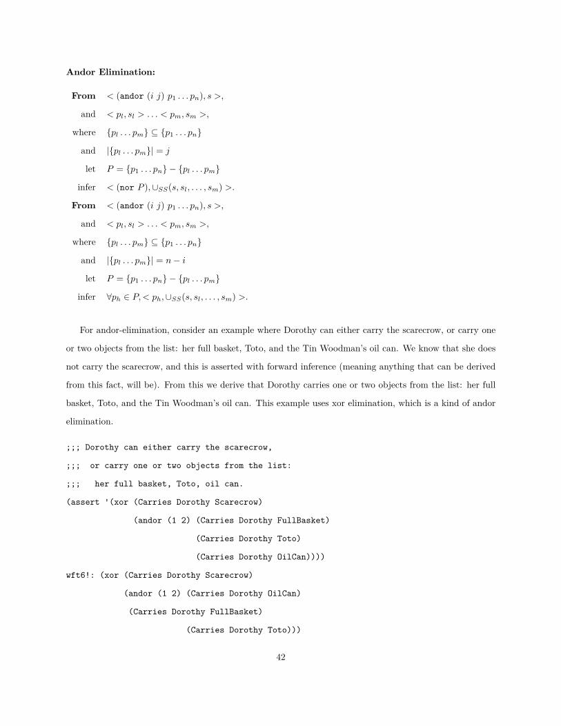
Andor Elimination:
From < (andor (i j) p1 . . . pn), s >,
and < pl, sl > . . . < pm, sm >,
where {pl . . . pm} ⊆ {p1 . . . pn}
and |{pl . . . pm}| = j
let P = {p1 . . . pn} − {pl . . . pm}
infer < (nor P ),∪SS(s, sl, . . . , sm) >.
From < (andor (i j) p1 . . . pn), s >,
and < pl, sl > . . . < pm, sm >,
where {pl . . . pm} ⊆ {p1 . . . pn}
and |{pl . . . pm}| = n− i
let P = {p1 . . . pn} − {pl . . . pm}
infer ∀ph ∈ P,< ph,∪SS(s, sl, . . . , sm) >.
For andor-elimination, consider an example where Dorothy can either carry the scarecrow, or carry one
or two objects from the list: her full basket, Toto, and the Tin Woodman’s oil can. We know that she does
not carry the scarecrow, and this is asserted with forward inference (meaning anything that can be derived
from this fact, will be). From this we derive that Dorothy carries one or two objects from the list: her full
basket, Toto, and the Tin Woodman’s oil can. This example uses xor elimination, which is a kind of andor
elimination.
;;; Dorothy can either carry the scarecrow,
;;; or carry one or two objects from the list:
;;; her full basket, Toto, oil can.
(assert '(xor (Carries Dorothy Scarecrow)
(andor (1 2) (Carries Dorothy FullBasket)
(Carries Dorothy Toto)
(Carries Dorothy OilCan))))
wft6!: (xor (Carries Dorothy Scarecrow)
(andor (1 2) (Carries Dorothy OilCan)
(Carries Dorothy FullBasket)
(Carries Dorothy Toto)))
42

;; Dorothy does not carry the Scarecrow. What can be derived from this?
(assert! '(not (Carries Dorothy Scarecrow)))
wft7!: (not "(Carries Dorothy Scarecrow)")
Since: wft6!: (xor (andor (1 2) (Carries Dorothy FullBasket)
(Carries Dorothy Toto)
(Carries Dorothy OilCan))
(Carries Dorothy Scarecrow))
and: wft7!: (not (Carries Dorothy Scarecrow))
I derived: wft4!: (andor (1 2) (Carries Dorothy FullBasket)
(Carries Dorothy Toto)
(Carries Dorothy OilCan)) by xor-elimination
Thresh Introduction:
From < p1, s1 > . . . < pk, sk >,
where k < i or k > j,
and ∃o such that < t1, o >∈ s1, . . . , < tk, o >∈ sk,
infer < (thresh (i j) p1 . . . pn), {< Λ(t1, . . . , tk), o >} >.
From < p1, s1 > . . . < pk, sk >,
where k < i or k > j,
and ¬∃o such that < t1, o >∈ s1, . . . , < tk, o >∈ sk,
infer < (thresh (i j) p1 . . . pn),makeExt(∪SS(s1 . . . sk)) >.
From < p1, s1 > . . . < pk, sk >,
where i < k < j,
and ∃o such that < t1, o >∈ s1, . . . , < tk, o >∈ sk,
infer < (not (thresh (i j) p1 . . . pn)), {< Λ(t1, . . . , tk), o >} >.
From < p1, s1 > . . . < pk, sk >,
where i < k < j,
and ¬∃o such that < t1, o >∈ s1, . . . , < tk, o >∈ sk,
infer < (not (thresh (i j) p1 . . . pn)),makeExt(∪SS(s1 . . . sk)) >.
From ∅,
infer < (not (thresh (0 0)), < Λ(∅), ∅ >>.
43
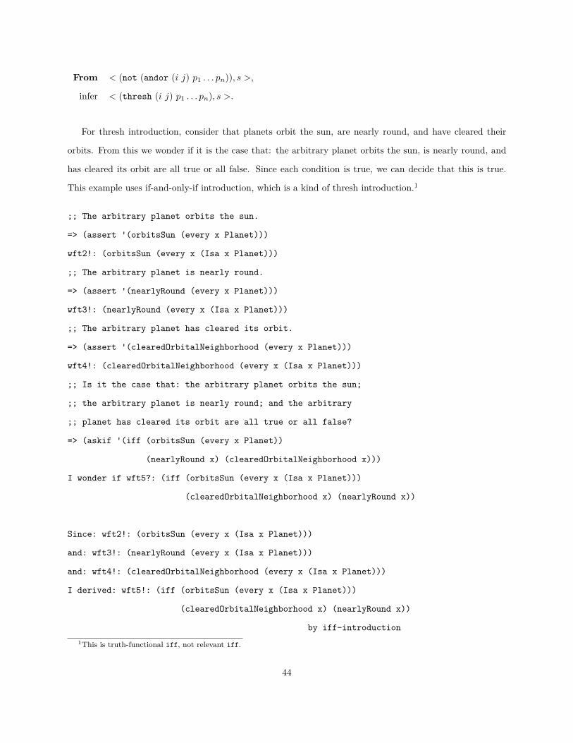
From < (not (andor (i j) p1 . . . pn)), s >,
infer < (thresh (i j) p1 . . . pn), s >.
For thresh introduction, consider that planets orbit the sun, are nearly round, and have cleared their
orbits. From this we wonder if it is the case that: the arbitrary planet orbits the sun, is nearly round, and
has cleared its orbit are all true or all false. Since each condition is true, we can decide that this is true.
This example uses if-and-only-if introduction, which is a kind of thresh introduction.1
;; The arbitrary planet orbits the sun.
=> (assert '(orbitsSun (every x Planet)))
wft2!: (orbitsSun (every x (Isa x Planet)))
;; The arbitrary planet is nearly round.
=> (assert '(nearlyRound (every x Planet)))
wft3!: (nearlyRound (every x (Isa x Planet)))
;; The arbitrary planet has cleared its orbit.
=> (assert '(clearedOrbitalNeighborhood (every x Planet)))
wft4!: (clearedOrbitalNeighborhood (every x (Isa x Planet)))
;; Is it the case that: the arbitrary planet orbits the sun;
;; the arbitrary planet is nearly round; and the arbitrary
;; planet has cleared its orbit are all true or all false?
=> (askif '(iff (orbitsSun (every x Planet))
(nearlyRound x) (clearedOrbitalNeighborhood x)))
I wonder if wft5?: (iff (orbitsSun (every x (Isa x Planet)))
(clearedOrbitalNeighborhood x) (nearlyRound x))
Since: wft2!: (orbitsSun (every x (Isa x Planet)))
and: wft3!: (nearlyRound (every x (Isa x Planet)))
and: wft4!: (clearedOrbitalNeighborhood (every x (Isa x Planet)))
I derived: wft5!: (iff (orbitsSun (every x (Isa x Planet)))
(clearedOrbitalNeighborhood x) (nearlyRound x))
by iff-introduction1This is truth-functional iff, not relevant iff.
44

Thresh Elimination:
From < (thresh (i j) p1 . . . pn), s >,
and PT = {< pl, sl > . . . < pm, sm >} such that |PT | ≥ i,
and PF = {< (not po), so >, . . . , < (not pp), sp >} such that |PF | = j − n− 1,
infer ∀pk ∈ ({p1, . . . , pn} − PT − PF ), < pk,∪SS(s, sl, . . . , sm, so, . . . , sp) >.
From < (thresh (i j) p1 . . . pn), s >,
and PF = {< (not pl), sl > . . . < (notpm), sm >} such that |PF | ≥ (n− j),
and PT = {< po, so >, . . . , < pp, sp >} such that |PT | = i− 1,
infer < (norP ),∪SS(s, sl, . . . , sm, so, . . . , sp) > where P = {p1, . . . , pn} − PT − PF .
To show thresh elimination in action, consider that a dog is carried by the person that owns it if and only
if that dog is scared, and Toto is a dog. We wonder what we can learn from that fact that Toto is scared.
Since Toto is a dog and Toto is scared, we can derive that Toto is carried by the person who owns Toto,
by both instantiating the arbitrary dog with Toto, and using if-and-only-if elimination (a type of thresh
elimination).
;; A dog is carried by the person who owns it, if and only if the dog is scared.
(assert '(iff (Scare (every x Dog)) (Carries (every y Person (Owns x)) x)))
wft6!: (iff (Scare (every x (Isa x Dog)))
(Carries (every y (Owns y x) (Isa y Person)) x))
;; Toto is a dog.
(assert '(Isa Toto Dog))
wft7!: (Isa Toto Dog)
;; Toto is scared. What can be derived from this?
(assert! '(Scare Toto))
wft8!: (Scare Toto)
Since: wft6!: (iff (Scare (every x (Isa x Dog)))
(Carries (every y (Owns y x) (Isa y Person)) x))
and: wft8!: (Scare Toto)
and: wft7!: (Isa Toto Dog)
I derived: wft11!: (Carries (every y (Isa y Person) (Owns y Toto)) Toto)
45

by iff-elimination
;; Therefore Toto is carried by his owner.
Numerical Entailment Introduction:2
From < c1, sc1 >, . . . , < cm, scm >
and ∀sj ∈ ders(sc1) . . . ders(scm), sj contains origin sets Oj which contain every cardinality i subset
of < a1, sa1 > . . . < an, san >,
then remove < a1, sa1 > . . . < an, san > from each Oj , and
infer < (=> i (setof a1 . . . an) (setof c1 . . . cm)),∪SS(all Ojs).
Consider that if Dorothy is scared then so is Toto, and that if Toto is scared he yelps. If it’s the case that
if Dorothy is scared, then Toto yelps, then Toto cares for Dorothy. We wonder if Toto cares for Dorothy.
Since if Dorothy is scared then so is Toto, and if Toto is scared he yelps, it follows that if Dorothy is scared,
Toto yelps, and therefore Toto cares for Dorothy.
;; If Dorothy is scared, then so is Toto.
(assert '(if (Scare Dorothy) (Scare Toto)))
wft3!: (if (Scare Dorothy) (Scare Toto))
;; If Toto is scared, he yelps.
(assert '(if (Scare Toto) (Yelp Toto)))
wft5!: (if (Scare Toto) (Yelp Toto))
;; If it's the case that if Dorothy is scared, then Toto yelps,
;; then Toto cares for Dorothy.
(assert '(if (if (Scare Dorothy) (Yelp Toto)) (CaresFor Toto Dorothy)))
wft8!: (if (if (Scare Dorothy) (Yelp Toto)) (CaresFor Toto Dorothy))
;; Does Toto care for Dorothy?
(askif '(CaresFor Toto Dorothy))
Since: wft5!: (if (Scare Toto) (Yelp Toto))
and: wft3!: (if (Scare Dorothy) (Scare Toto))2Note, the full numerical entailment introduction rule has not yet been implemented. The cases for i = 1 and i = n have
thus far been implemented.
46

I derived: wft6!: (if (Scare Dorothy) (Yelp Toto)) by if-introduction
Since: wft8!: (if (if (Scare Dorothy) (Yelp Toto)) (CaresFor Toto Dorothy))
and: wft6!: (if (Scare Dorothy) (Yelp Toto))
I derived: wft7!: (CaresFor Toto Dorothy) by if-elimination
Numerical Entailment Elimination:
From < (=> i (setof a1 . . . an) (setof c1 . . . cm)), s >
and at least i of the antecedents, < aj , sj > . . . < ak, sk >
infer < c1,∪SS(s, sj , . . . , sk) >, . . . , < cm,∪SS(s, sj , . . . , sk) >
To show numerical entailment elimination, consider that if Dorothy is chased, or Toto is being chased,
Toto is scared, and that Dorothy is being chased. We can then wonder if Toto is scared and find that the he
is. This example makes use of or-entailment elimination.
;; If Dorothy is chased or Toto is being chased, Toto is scared.
(assert '(=v> #{(Chase Dorothy) (Chase Toto)} (Scare Toto)))
wft4!: (=v> #{(Chase Dorothy) (Chase Toto)} (Scare Toto))
;; Dorothy is being chased.
(assert '(Chase Dorothy))
wft1!: (Chase Dorothy)
;; Is Toto scared?
(askif '(Scare Toto))
Since: wft4!: (=v> #{(Chase Dorothy) (Chase Toto)} (Scare Toto))
and: wft1!: (Chase Dorothy)
I derived: wft2!: (Scare Toto) by numericalentailment-elimination
CSNePS does not yet implement the standard rule of negation introduction via reductio ad absurdum3,
but does implement negation elimination through double negation elimination.
Negation Elimination:
3See Section 9.2.2.3 in the chapter on future work for an explanation of why.
47

From < (not (not A)), s >,
infer < A,Λs(s) >.
To show negation elimination consider that it is not the case that Obama is not president. When it is
asked if Obama is president, this is found to be true, since “it is not the case that Obama is not president”
is a double-negative.
;; It's not the case that Obama is not president.
(assert '(not (not (isPresident Obama))))
wft3!: (not (not (isPresident Obama)))
;; Is Obama president?
(askif '(isPresident Obama))
Since wft3!: (not (not (isPresident Obama)))
I derived: wft1!: (isPresident Obama) by negation-elimination
Closure introduction and elimination rules are directly adapted from (Shapiro, 2004).
Closure Introduction:
From < A, s >
where A contains quantified term x
infer < (close x A), hypsToDers(s) >.
Both closure introduction and closure elimination are implemented via rewrite rules in the object lan-
guage, which will be discussed further in Section 3.2. As seen in the following example (and the one for
closure elimination), rewrite rules make use of if-and-only-if rules added to the knowledge base.
;; The arbitrary mammal is an animal.
=> (assert '(Isa (every x (Isa x Mammal)) Animal))
wft2!: (Isa (every x (Isa x Mammal)) Animal)
=> (askif '(close (x) (Isa (every x (Isa x Mammal)) Animal)))
I wonder if wft3?: (close (x) (Isa (every x (Isa x Mammal)) Animal))
Since: wft4!: (iff (Isa (every x (Isa x Mammal)) Animal) (close (x) (Isa x Animal)))
48

and: wft2!: (Isa (every x (Isa x Mammal)) Animal)
I derived: wft3!: (close (x) (Isa (every x (Isa x Mammal)) Animal)) by iff-elimination
Closure Elimination:
From < (close x A), s >,
infer < A, hypsToDers(s) >.
;; The arbitrary mammal is an animal. What can be derived from this?
=> (assert! '(close x (Isa (every x (Isa x Mammal)) Animal)))
wft3!: (close (x) (Isa (every x (Isa x Mammal)) Animal))
Since: wft4!: (iff (Isa (every x (Isa x Mammal)) Animal) (close (x) (Isa x Animal)))
and: wft3!: (close (x) (Isa (every x (Isa x Mammal)) Animal))
I derived: wft2!: (Isa (every x (Isa x Mammal)) Animal) by iff-elimination
Generic terms have previously been defined as atoms containing open arbitrary terms. The different
components of a generic term may be made more concrete: a generic term is a term which has one or more
generic or arbitrary subterms ({g1, . . . , gj}, and {a1, . . . , ak}, respectively), and possibly some subterms with
no open arbitraries, {p1, . . . , pi}. Therefore, we write a genericR as (R {p1, . . . , pi} {g1, . . . , gj} {a1, . . . , ak}).
Any number of the {g1, . . . , gj}, and {a1, . . . , ak}may be instantiated to create a new generic with the applied
substitution.
Generic Instantiation:
From < (R {p1, . . . , pi} {g1, . . . , gj} {a1, . . . , ak}), s >,
where there are compatible substitutions {σg1, . . . , σgj , σa1, . . . , σak},
then let σR = the combination of all σg’s and σa’s
and P = σR(R {p1, . . . , pi} {g1, . . . , gj} {a1, . . . , ak}),
and sP = ∪SS(all terms in σR),
infer < P, sP >.
Generic instantiation by a constant has already been seen in the thresh elimination example, so here it
will be shown how a generic can instantiate another. Consider that the arbitrary lion eats the arbitrary
animal. From the fact that the arbitrary antelope is an animal, what can we derive? It is clear that since
49

the arbitrary antelope is an animal, and the arbitrary lion eats the arbitrary animal, the arbitrary lion eats
the arbitrary antelope.
;; The arbitrary lion eats the arbitrary animal.
(assert '(eats (every x (Isa x Lion)) (every y (Isa y Animal))))
wft3!: (eats (every x (Isa x Lion)) (every y (Isa y Animal)))
;; The arbitrary antelope is an animal. What can we derive from this?
(assert! '(Isa (every z Antelope) Animal))
wft5!: (Isa (every z (Isa z Antelope)) Animal)
Since: wft3!: (eats (every x (Isa x Lion)) (every y (Isa y Animal)))
and: wft5!: (Isa (every z (Isa z Antelope)) Animal)
I derived: wft6?: (eats (every x (Isa x Lion)) (every z (Isa z Antelope))) by generic-instantiation
3.1.3 Structural Rules
The only exclusively structural rule used in CSNePS is one that eliminates negated closures. A term that
contains an arbitrary x, is closed over x, and negated must treat x as an indefinite term. A term that contains
an indefinite x, is closed over x, and negated must treat x as an arbitrary term. The negated closure rule
below allows for these transformations.
Negated Closure:
From < A, s >,
which has a subterm (not (close x B)),
where x is the variable for arbitrary term arbx,
infer < {(some x R(arbx))/arbx,B/(close x B)} applied to A, s >.
From < A, s >,
which has a subterm (not (close x B)),
where x is the variable for indefinite term indx,
infer < {(every x R(indx))/indx,B/(close x B)} applied to A, s >.
The implementation of this rule will be explored in more detail in the following section.
50

3.2 Rewrite Rules
Some rules of inference are particularly difficult to implement in IGs because negations alter the behavior
of inner logical connectives. For this reason, we have implemented a series of “rewrite rules” for these cases.
These rules are not true rewrite rules, since they do not replace the expression written by the user. Instead,
the portion of the expression which can be re-expressed is made logically equivalent to the original using
iff. This way, the user’s entered term is still in the KB, and a rule easier to reason about is present as well.
The rules which require re-expression are negated closure, negated andor, and negated thresh.
There are several advantages to this approach of re-expression. Inference Graphs make the assumption
that it is possible to match all terms which should communicate during inference with each other. The rules
surrounding such a match become very cumbersome should, for example, a negated thresh, and equivalent
andor be used in the KB. The automatic generation of the equivalency at assert-time makes the matching
trivial. Another concern is that negated closures change the behavior of the closed-over quantified term.
This would force all quantified terms to to act the same until some decision point is reached. This forces a
great deal of overhead in the collection of instances for indefinite terms, which otherwise would do no such
thing.
3.2.1 Closures
In inference, closures exhibit themselves most strongly when combined with negation. Consider the following
two terms (from (Shapiro, 2004)):
1. (not (White (every x (Isa x Sheep))))
2. (not (close x (White (every x (Isa x Sheep)))))
The first is intended to mean that “every sheep is not white”, and the second that “it is not the case that
every sheep is white”. The close relation has the effect of limiting the scope of the closed variable. When
used in combination with a negation, the effect is that of negation on standard FOL quantifiers, as in:
¬∀xR(x) ≡ ∃x¬R(x), and
¬∃xR(x) ≡ ∀x¬R(x).
This equivalence is made explicit using a rewrite rule. In the second case above, (not (close x (White
(every x (Isa x Sheep))))) is added to the KB, but so is:
51

(iff (not (close x (White (every x (Isa x Sheep))))) (not (White (some x () (Isa x
Sheep))))
3.2.2 andor and thresh
As with closures, the andor and thresh connectives act differently when negated. As defined in the imple-
mented rules of inference, they act as the opposite connective.
Consider the proposition that Eric believes that if a fruit is edible, it is not the case that that fruit is
any of: poisonous, shrived, or rotten.
(Believes Eric (if (Edible (every x Fruit))
(not (or (Poisonous x) (Shriveled x) (Rotten x)))))
This proposition makes use of a negated andor, since (or ...) is equivalent to (andor (1 3) ...) in
this case (meaning at least one and at most three of the arguments are true). We therefore rewrite the or
to use thresh, as follows:
(iff
(not (or (Poisonous (every x Fruit)) (Shriveled x) (Rotten x)))
(thresh (1 3) (Poisonous (every x Fruit)) (Shriveled x) (Rotten x)))
When this proposition is being built into CSNePS, it will convert (thresh (1 3) ...) to (nor ...),
since none of the arguments may be true. So the final translation is:
(iff
(not (or (Poisonous (every x Fruit)) (Shriveled x) (Rotten x)))
(nor (Poisonous (every x Fruit)) (Shriveled x) (Rotten x)))
Note that we do not rewrite the entire proposition, but rather only the parts which require it. Using this
rewrite, our original expression means that Eric believes that if a fruit is edible, that fruit is neither poisonous,
nor shriveled, nor rotten. The rewriting of (not (thresh ...)) to (andor ...) works similarly.
3.3 Implementation Decisions Regarding LA
CSNePS and IGs make two important decisions in implementing LA, solving issues and enhancing what was
defined in (Shapiro, 2004). The first of these deals with the possibility of having more than one arbitrary
52

term with the same restriction set, and how to ensure that terms that should be taken to be identical (or
not) are treated as such. The second is really a group of enhancements, designed to make using LA more
pleasant through the introduction of some syntactic sugar.
3.3.1 Sameness of Quantified Terms
The issue of when quantified terms may be bound to the same term in a knowledge base is one that requires
some thought. Scott Fahlman in his 1979 book on NETL (Fahlman, 1979) discussed the difficulty in capturing
the intended meaning of (hates Arbitrary-Elephant Arbitrary-Elephant), where Arbitrary-Elephant
represents the arbitrary elephant. There are three possible meanings of this:
1. The arbitrary elephant hates itself.
2. The arbitrary elephant hates all other elephants.
3. The arbitrary elephant hates all elephants (including itself).
To solve this problem he introduced the other operator to distinguish between two arbitraries. Item 1
stays (hates Arbitrary-Elephant Arbitrary-Elephant), item 2 becomes (hates Arbitrary-Elephant
Other-Arbitrary-Elephant), and item 3 becomes the conjunction of the two.
We solve this problem for arbitraries through the use of LA’s variable labels. The use of different variable
labels for otherwise identical arbitrary terms indicates that the user intended the two arbitraries to be
different. Below we give the LA representation for each of the above three intended meanings:
1. (hates (every x (Isa x Elephant)) x)
2. (hates (every x (Isa x Elephant)) (every y (Isa y Elephant)))
3. (hates (every x (Isa x Elephant)) #{x (every y (Isa y Elephant))})
In LA, arbitrary terms are not the only ones which users may wish to explicitly make different from one
another. Indefinite individuals which use different variable labels as described above are also assumed to
be different. For example, in (hates (some x (Isa x Elephant)) (some y (Isa y Elephant))), some
elephant hates some other elephant, the two indefinite Elephants are assumed to be different because of their
different variable labels. If it is desired that an indefinite be different from an arbitrary, the issue is more
complex (as the two must, by definition, have different variable labels).
53

Different types of quantified terms with different variable labels are able to be bound to the same term
unless it is explicitly noted that they should not. Consider that every elephant hates some elephant: (hates
(every x (Isa x Elephant)) (some y (Isa y Elephant))). Since there are two different types of quan-
tified terms in action, it’s necessary that x and y have different variable labels. In this case, x and y may both
be bound to the same term. In order to make explicit that x and y should not be bound to the same term,
we introduce the (notSame qj1 . . . qjk) relation. The notSame relation is special (i.e., it is not represented
in the graph like other restrictions) and can be used to ensure that any two quantified terms are bound
to different terms. The naming apart of arbitrary and indefinite variables as described above is simply a
shortcut for using the notSame relation. The user could have, for example, written item 2 above as:
(hates (every x (Isa x Elephant)) (every y (Isa y Elephant) (notSame x y)))
with the identical meaning.
3.3.2 Syntactic Sugar
Over time, writing expressions in LA can become rather tiring (as in just about any logic), as the syntax
is often a bit too verbose for the situation at hand. For this reason we introduce four abbreviations that
may be used when writing quantified terms. The system automatically converts the abbreviations to their
un-abbreviated form.
1. The restriction (Isa x C), where C is a category, may be written simply as C.
Ex: The arbitrary term written (every x (Isa x Person) (Isa x Officer)) may be rewritten
simply as (every x Person Officer).
2. A relational term P abbreviates (P x), where x is the variable for the immediately enclosing quantified
term.
Ex: The arbitrary term written (every x (Isa x Person) (Alive x)) may be rewritten as: (every
x Person Alive).
3. A relational term (R y1 . . . yn) abbreviates (R x y1 . . . yn), where x is the variable for the immediately
enclosing quantified term, unless x ∈ {y1 . . . yn}, or the number of arguments given for R already equal
its maximum allowable.
Ex: The arbitrary term written (every x (eats x Grain)) may be rewritten as: (every x (eats
Grain)).
54
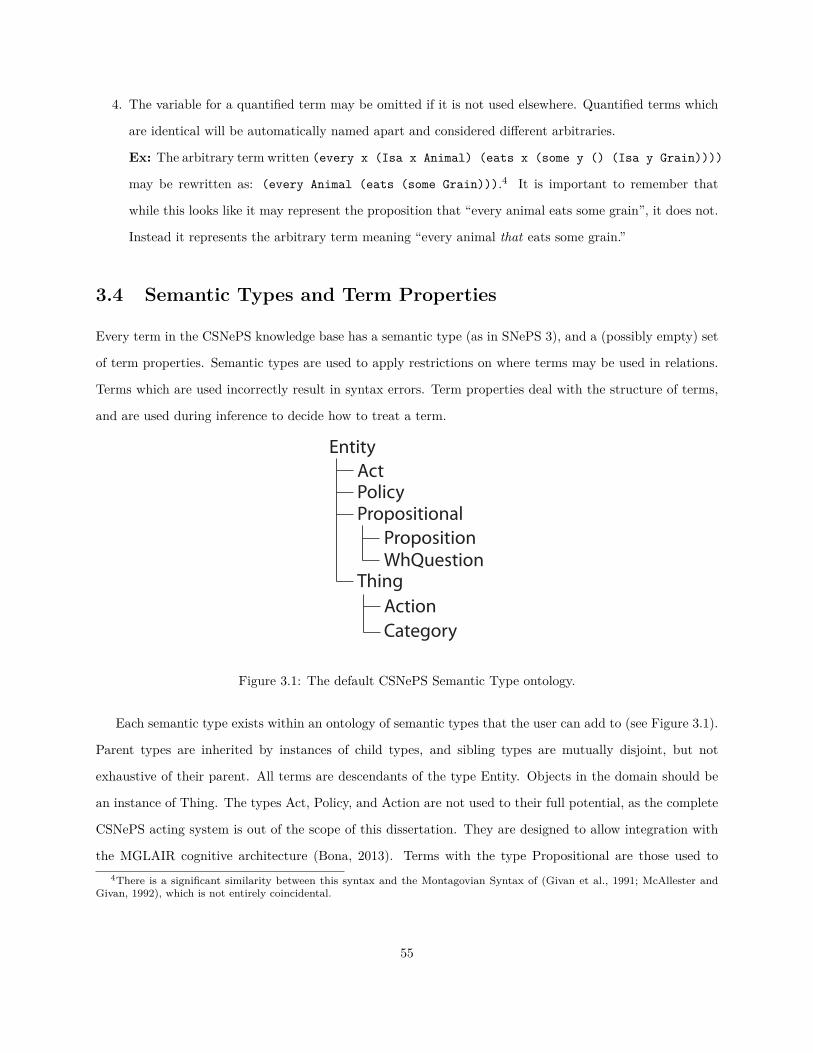
4. The variable for a quantified term may be omitted if it is not used elsewhere. Quantified terms which
are identical will be automatically named apart and considered different arbitraries.
Ex: The arbitrary term written (every x (Isa x Animal) (eats x (some y () (Isa y Grain))))
may be rewritten as: (every Animal (eats (some Grain))).4 It is important to remember that
while this looks like it may represent the proposition that “every animal eats some grain”, it does not.
Instead it represents the arbitrary term meaning “every animal that eats some grain.”
3.4 Semantic Types and Term Properties
Every term in the CSNePS knowledge base has a semantic type (as in SNePS 3), and a (possibly empty) set
of term properties. Semantic types are used to apply restrictions on where terms may be used in relations.
Terms which are used incorrectly result in syntax errors. Term properties deal with the structure of terms,
and are used during inference to decide how to treat a term.
EntityActPolicyPropositional
PropositionWhQuestion
ThingActionCategory
Figure 3.1: The default CSNePS Semantic Type ontology.
Each semantic type exists within an ontology of semantic types that the user can add to (see Figure 3.1).
Parent types are inherited by instances of child types, and sibling types are mutually disjoint, but not
exhaustive of their parent. All terms are descendants of the type Entity. Objects in the domain should be
an instance of Thing. The types Act, Policy, and Action are not used to their full potential, as the complete
CSNePS acting system is out of the scope of this dissertation. They are designed to allow integration with
the MGLAIR cognitive architecture (Bona, 2013). Terms with the type Propositional are those used to4There is a significant similarity between this syntax and the Montagovian Syntax of (Givan et al., 1991; McAllester and
Givan, 1992), which is not entirely coincidental.
55

express Propositions and “wh-” style queries (WhQuestion, see Section 2.4). Only Propositions may be
asserted (taken to be true) in the knowledge base.
A term is given a semantic type based on its usage. Each argument in a CSNePS expression is associated
with a semantic type. As a term is used in argument positions with different types, the type of the term is
adjusted downward.
For example, consider the addition of Organism as a subtype of Entity, and Mammal as a subtype of
Organism. Also consider two unary relations: hasParent, which takes an Organism argument, and hairy
which takes a Mammal argument. As we’ve said, non-quantified terms may have their types inferred, so it
is allowed to say (hasParent Alex), at which point Alex is determined to be an Organism, and later say
(hairy Alex) at which point Alex is determined to be a Mammal.
The semantic type of arbitrary terms may not change after they have been created. Arbitrary terms
have internal and external type restrictions. The internal restriction is the lowest type corresponding to a
categorization in the term’s restrictions. The external restriction is the type of the argument position they
are used in. Their final type is specified by the internal restriction, and must always agree with the external
restriction. This decision was made to ensure soundness of the logic as items are added to the KB after
inference has already occurred. Indefinite terms, which act like constants, do not share this property.
Continuing the above example, it’s clear that the arbitrary in (hasParent (every x (Isa x Organism)))
should not be able to be used in the hairy relation, since the arbitrary matches all Organisms, and the def-
inition of hairy said that only Mammals qualified. So, it is legal to say that (hairy (every x Mammal)),
but not (hairy (every x Organism)), since the internal restrictions do not allow it.
In addition to having a semantic type, each term has a set of properties. The two properties currently
made use of by the Inference Graph are Generic and Analytic. Generic terms are, as we’ve discussed, those
with open variables. They need not be a proposition though, the generic parent of someone: (parent (some
x Person)) where the parent relation may be an Entity, is an equally valid generic as the generic rule that
the parent of someone has a child: (hasChild (every x (parent (some y Person)))).
3.5 Question Answering
As discussed in Section 2.4, there are two types of questions we are concerned with answering using IGs —
specific, and generic questions. The same machinery will be used to answer both of these types of questions.
The distinction we will make is between questions which may be answered with yes or no, such as “Is Mary
56
at home?” or “Are all children at home?”, and what are often called wh-questions, such as “Who is at
home?”
Since CSNePS implements a term logic, yes-or-no questions such as “Is Mary at home?” are answered
with the satisfying term itself, (e.g., “Mary is at home.”) rather than yes or no (or true or false). The open
world assumption means that if no answer is forthcoming to the asked question, than none is returned to
the user.
3.5.1 Wh-Questions
Wh-questions may have no answers, one answer, or many answers. In order to answer wh-questions, a new
type of quantified term, called a query term, is introduced. A query term acts identically to an arbitrary,
but restricts the semantic type of a containing expression. While the query expression may on the surface
look like a Proposition, it is clearly not, as it contains no proposition. Groenendijk and Stokhof call the
semantic content of interrogative expressions “Questions” (Groenendijk and Stokhof, 2008). Since our query
variables cover only wh-questions, we call the semantic type for them WhQuestion. The similarity between
the WhQuestion and the Proposition is not lost on us though, both are direct descendents of the semantic
type Propositional. One reason for creating a new type of quantified term, rather than re-using arbitraries
for this purpose, is an issue mentioned in (Burhans and Shapiro, 2007) — often humans ask questions about
generics, and it’s inappropriate in those cases to return instances of the generic. This allows us to separate
the question “Are all children at home?” which uses an arbitrary term, from “Which children are at home?”
which uses a query term.
Syntactically, query terms are expressed much like other quantified terms. CSNePS allows such questions
to be asked by using the askwh function,5 and giving it a CSNePS expression as an argument, with one or more
of the expression’s slots filled by a query term, expressed as (?x r1 . . . rn), where r1 . . . rn are restrictions.
When no special restrictions are desired by the user, they may use a question-mark prefixed placeholder,
such as ?x, instead of writing the full quantified term.
When a question is asked of the system, the question asked is added to the knowledge base, and backward
inference is performed upon it. Instead of asserting instances found as a generic term would, it caches them
and returns them to the user. Since questions are added to the KB, it is possible to reason about questions
asked of the system, though we have not yet explored this in detail.
5The complete CSNePS syntax and definition of functions is available in the CSNePS manual, distributed with CSNePS.See Section 9.3 about availability.
57
Chapter 4
Term Unification and Matching
As previously described, inference operations in the IG are carried out through the transmission of messages
through channels, and their combination in nodes. Many of the channels within the graph are added between
terms that match each other. When a term is added to the graph, it is determined whether the added term
and any other terms might need to communicate during inference. This determination is accomplished
through the match process. This process occurs in two phases: first, the added term is unified with all
other terms in the graph; then the resulting substitutions are checked for appropriate type and subsumption
relationships.
In order to efficiently perform the matching operation, we make use of term trees to index the KB and
efficiently perform one-to-many unification, detailed in Sections 4.1 and 4.2. Since sets of terms may need
to be unified, a flavor of set unification has been developed, presented in Section 4.3. Finally, the match
operation, which encompasses unification and other relationships, is discussed in Section 4.4.
4.1 Term Trees
A term tree is a discrimination tree for terms, acting as an index of the knowledge base. Term trees contain
two types of nodes: t-nodes, which represent terms; and f-nodes, which represent function symbols (or other
terms in function position).
Term trees are created by examining each term in the knowledge base. Terms are traversed using a
post-order tree traversal. In the term being traversed, leaf nodes are literals, and inner nodes are molecules.
When a molecular node is visited on the way down, an f-node is created for it. When it is visited on the
58

way back up the tree, a t-node is created for it. T-nodes are created for each literal. Edges connect nodes
in the order of traversal. Nodes are created for arbitrary and indefinite terms, but not their restriction sets.
For example, the term (R (f a b) (every x (P x))) becomes the “tree” (really, chain):
R->f->a->b->(f a b)->(every x (P x))->(R (f a b) (every x (P x))).
R and f in this example are f-nodes, and the others are t-nodes.
When a new term is added to a term tree, the existing term tree and the new term are traversed in
parallel. At the point where the two differ, a new branch of the term tree is created. This is similar to the
method used for creating the RETE net alpha network.
Term trees are particularly easy to produce, since quantified terms in LA need not be named apart,1 as
variables need to be in other FOLs. Therefore adding a term to the term tree requires only a single walk
through a term linear in time with the total number of literals and function symbols used in the term.
Term trees are most closely related to downward substitution trees (Hoder and Voronkov, 2009) (DSTs),
which have one or more substitutions instead of a single term in each of their nodes. The lack of variable
renaming in LA accounts for why term trees may use terms and function symbols instead of substitutions.
DSTs may contain multiple substitutions at a single node, while a term tree cannot have multiple terms or
function symbols at a single node. This is a space/time tradeoff, since a DST may need to spend the time
splitting a node, while a term tree does not, but the term tree must use more memory for the extra branches
of the tree. Given the abundance of cheap memory available today, we feel the extra space usage is not of
concern.
P3 arb1
arb1
arb1
arb2
wft3
(f arb1)
(f arb2)
a
f1
wft1
wft2
a
a
Figure 4.1: A term tree for the terms: wft1: (P arb1 (f arb1) a), wft2: (P arb1 (f arb2) a), andwft3: (P arb1 arb1 a).
Figure 4.1 is a term tree built for the three terms wft1: (P arb1 (f arb1) a), wft2: (P arb1 (f1Remember, there is only one arbitrary with a particular set of restrictions (including the special, and often implicit, notSame
restriction). Using the terms identifier (e.g., arb1) is sufficient naming apart. Indefinite terms can never be assumed to beequivalent, so the CSNePS build system creates a new (already named-apart) indefinite each time one is encountered.
59
arb2) a), and wft3: (P arb1 arb1 a). Our unification algorithm does not examine the restrictions of
arbitrary terms (this is an issue of subsumption, not unification, so is handled later), so we won’t worry
about the full structure of arbitrary terms throughout this example, only labeling them using names like
arb1. Function symbols (f-nodes) are superscripted with their arity. The final node in each chain (shown as
wft1− wft3) represents the propositions being matched to in the KB.
4.2 Unification
Hoder and Voronkov (2009) have shown that the Robinson unification algorithm (Robinson, 1965), along with
a slight modification of it to solve the exponential case, called PROB, are the fastest unification algorithms
on an assortment of real-world problems when used in combination with downward substitution trees. The
Robinson and PROB algorithms apply substitutions at each intermediate step of the algorithm, and, in the
process, generate a lot of intermediate structures that need to be cleaned up by garbage collection later.
As discussed in (Norvig, 1991), there are two common solutions to this: the Prolog method of representing
logic variables as cells to be updated destructively, and maintaining a history for backtracking; and building
up the substitutions as the algorithm progresses, but delaying the application of the substitution until the
end. The algorithm we use is of this second variety. Again as (Norvig, 1991) points out, this algorithm is
widely used in several AI texts, and is used in the MRS (Russell, 1985) reasoning system. It is also used in the
core.unify library (Fogus, 2014), which we base our implementation on. This algorithm has the possibility
to be faster than PROB, especially in cases where the number of variables is much less than the length of
the patterns being matched.
Our unification algorithm is given in Algorithm 4.1, without the portions that flatten recursive substitu-
tions, and test the bindings, as these are uninteresting in the current discussion.
Unification can be seen as a series of comparisons between two predicates with the additional step of
creating and maintaining relevant substitutions at each comparison. The series of comparisons can be “un-
rolled” into a chain of comparisons, which match up with the structure of the term tree. For this reason, the
exact algorithm used for the unification operation itself is important only from a performance point of view
— any unification algorithm that can be un-rolled in this fashion may be used. It can be easily seen that the
unification algorithm we make use of is of this variety: if s and t are two terms of arity i to be unified, and s′
and t′ are identical to s and t but with extra arguments s1 and t1, respectively (and therefore they have arity
i+ 1), then by examining the algorithm it’s obvious that unify(s′, t′, {}) = unify(s1, t1, unify(s, t, {})).
60

Algorithm 4.1 Our implemented unification algorithm, as discussed in (Norvig, 1991), with minor modifi-cations to operate on CSNePS terms. Note that while really molecular CSNePS terms have set arguments,we’re ignoring sets for the moment.function unify(x, y, subst)
if x = y thenreturn subst
else if subst = nil thenreturn nil
else if varterm?(x) thenunify-variable(x, y, subst)
else if varterm?(y) thenunify-variable(y, x, subst)
else if list?(x) and list?(y) thensx← rest(x)sy ← rest(y)fx← first(x)fy ← first(y)fsubst← unify(fx, fy, subst)return unify(sx, sy, fsubst)
elsereturn nil
end ifend functionfunction unify-variable(var, term, subst)
if var = term thenreturn subst
else if bound?(var, subst) thenbinding ← get(var, subst)return unify(binding, term, subst)
else if varterm?(term) and bound?(term, subst) thenbinding ← get(term, subst)return unify(var, binding, subst)
else if occursIn?(var, term, subst) thenreturn nil
elsereturn assoc(var, term, subst)
end ifend function
61

The term tree allows unification to occur simultaneously for multiple predicates with shared prefixes,
only performing unification on them separately when they differ. Given that unification is among the most
expensive processes that occur in an inference system, this provides a significant performance advantage over
simply performing unification against each term in the KB independently.
Terms to be unified against the existing term tree flow through the term tree, along with a substitution
generated from the in-progress unification, initially empty. T-nodes perform unification between the node’s
term, and the appropriate part of the passing term, given the substitution already produced. Failure occurs
in a branch when unification usually would (e.g., failure of the occurs check, or two different constant terms).
F-nodes ensure that the passing term has the appropriate function symbols in the appropriate positions (or,
a variable where that function symbol should go, indicating that the passing term may proceed to that
function symbol’s corresponding t-node for unification). Should a term and its substitution reach the t-node
at a leaf of the tree, it unifies with the wft that that leaf stands for, with that substitution. The algorithm
is presented more formally in Algorithm 4.2.
Theorem 4.1. Algorithm 4.2 will result in a most general unifying substitution wherever possible.
Proof. We will show that given a term, T , and term tree and substitution, that the result is a set of most
general unifying substitutions, one for each term in the term tree that unifies with T . We will start by
showing this is true for a term “tree” containing only a single term, then show that it is a trivial extension
to operate on the entire tree.
Invariant: At position i in term T , and node j in the term tree, subst represents a most general unifier for
positions 0 . . . i− 1 of T and 0 . . . j− 1 of the term tree, where 0 is the root of the tree, and 0 . . . j represents
a path through the tree.
Base Case: For i = 0, the examination of the nodes has not yet begun, so subst = {}.
Inductive Step: At position n in term T and node m in the term tree, subst is a most general unifier for
positions 0 . . . n− 1 in T and 0 . . .m− 1 in the term tree. There are six cases to consider:
1. n is a function symbol, and m is an f-node.
2. n is an arbitrary or query variable, and m is an f-node.
3. n is a non-arbitrary or query variable term, and m is an f-node.
4. n is a function symbol, and m is an t-node.
5. n is an arbitrary or query variable, and m is an t-node.
62

Algorithm 4.2 The algorithm for traversing a term and unifying it with the term tree. The argument[t|Term] indicates a post-order traversal of Term, as was done in creation of the term tree itself. t is thecurrent sub-term being considered, and Term is the unexplored portion of the term. Unify is a call to theunification algorithm of (Norvig, 1991), as described earlier.function treeUnify([t|Term], node, subst)
if isFsymbol(t) and isFNode(node) thenif t = getFSymbol(node) then
return the set of:for all children c of node do
treeUnify(Term, c, subst)end for
elsereturn FAIL
end ifelse if (isArbitrary(t) or isQvar(t)) and isFNode(node) then
return the set of:for all t-nodes, tnode, for node do
treeUnify(t, tnode, subst)end for
elsent← getTerm(node)subst← unify(t, nt, subst)if subst = nil then
return FAILelse if Term is empty then
return [node subst]else
return the set of:for all children c of node do
treeUnify(Term, c, subst)end for
end ifend if
end function
63
6. n is a non-arbitrary or query variable term, and m is an t-node.
These are each handled by the algorithm, maintaining the invariant, as follows:
1. If the function symbols are identical, then proceed to n+ 1 and m+ 1 with subst. If not, then fail.
2. Jump to the t-node for m since m represents the function symbol for the larger term indicated by it’s
t-node, and begin testing these six cases again.
3. A call to unify will be attempted, and as the unification algorithm is known to be correct, will result
in proceeding to n+ 1 and m+ 1 with an updated subst if it succeeds, otherwise a failure state.
4. This will result in failure when unify is attempted.
5. A call to unify will be attempted, and as the unification algorithm is known to be correct, will result
in proceeding to n+ 1 and m+ 1 with an updated subst if it succeeds, otherwise a failure state.
6. A call to unify will be attempted, and as the unification algorithm is known to be correct, will result
in proceeding to n+ 1 and m+ 1 with an updated subst if it succeeds, otherwise a failure state.
Therefore, in all non-failure states, the invariant is maintained.
This may be extended to the case of multiple items in the tree, with the added condition that instead of
proceeding to m+ 1 in the tree, all children of m must be considered.
Figure 4.2 presents two examples of attempted unification, given the existing term tree created in the
previous section (Figure 4.1). In Figure 4.2a, it is shown that wft4 unifies with both wft1 and wft2,
but not wft3. wft4 enters the term tree at P 3 with an empty substitution, {}. Since wft4 also has the
function symbol P with arity 3, it passes to the next node. arb1 is compared against (g arb3). These unify
with the substitution {(g arb3)/arb1} (read, “(g arb3) for arb1”). wft4 along with the substitution {(g
arb3)/arb1} pass now along two paths — to f1 and arb1. At arb1 unification fails, since the existing
substitution {(g arb3)/arb1} and new substitution {(f (g arb4))/arb1} may not be combined. At the
f-node f1, it is found that wft4 also has the function symbol f of arity 1 in its second argument position,
and it passes on to both arb1 and arb2. This process continues all the way to the f-nodes for wft1 and
wft2. 4.2b shows a second example where wft3 unifies with the given term, and wft1 and wft2 fail.
In practice, unification is slightly more difficult than this. When two terms, ti and tj , are unified, instead
of producing an mgu, a factorization is produced that contains bindings for each of the terms being unified.
While the exact process by which these bindings are produced is available in (McKay and Shapiro, 1981),
64

Test uni�cation of:
FAIL
Test uni�cation of:
P3 arb1
arb1
arb1
arb2a)
wft3
(f arb1)
(f arb2)
a
{g(arb3)/arb1}
{g(arb3)/arb1, arb3/arb4}
{g(a)/arb1, a/arb4}
{b/arb1}
P3 arb1b)
{b/arb1}
{b/arb1, a/arb5}
FAIL
{g(arb3)/arb1, g(arb4)/arb2}
{g(arb3)/arb1, g(a)/arb2, a/arb4}
wft4: (P (g arb3) (f (g arb4)) arb4)
f1
{g(arb3)/arb1}
wft1
wft2
a
a
{g(arb3)/arb1, arb3/arb4}
{g(arb3)/arb1}{g(arb3)/arb1, g(arb4)/arb2}
{g(arb3)/arb1}
arb1
arb2
(f arb1)
(f arb2)
f1
wft1
wft2
a
a
arb1 wft3a
{b/arb1}
wft5: (P b b arb5)
{}
{}
Figure 4.2: Two examples of unification. In part a, it is found that wft4 unifies with both wft1 and wft2,but not wft3, since arb3 and arb4 are different. In part b, it is found that wft5 unifies with wft3 butneither wft1 nor wft2, since b cannot unify with a functional term.
65

the main idea is that unification is performed as usual, except that instead of forming a single substitution,
two are formed — σi and σj — such that all and only quantified terms in ti are given bindings in σi, and
all and only quantified terms in tj are given bindings in σj . These substitutions allow for the creation of
structures within the channels, as will be discussed in the next chapter.
4.3 Set Unification
Formulating the set unification problem is difficult, and is dependent upon the ultimate goal of the unification.
Some formulations (Dovier et al., 2006) aim to find a unifier that makes the two sets equivalent, therefore
requiring the sets to be of the same size. We concern ourselves more with unifying specific elements between
the two sets. The definition of set unification used in this dissertation is given below.
Definition 4.2. Two sets S1 and S2 where |S1| ≤ |S2|, unify if every x ∈ S1 unifies2 with some unique
y ∈ S2. �
The formulation presented here is limited in that each term in one set may unify with only one set element
in the opposite set in each solution, and each result necessarily has the cardinality of the smaller set. It is
currently undetermined whether these limitations are significant and need to be addressed in the future.
In order to determine if two sets unify, and find their mgu, it is clear from the definition of set unifi-
cation that some combinatorial algorithm will be necessary. To make this more concrete, let’s consider an
example. Using the above definition of set unification, the two sets s ={arb1, arb2, (caregiver arb2)}
and t ={arb3, Alex} have four unifiers:
1. {Alex/arb1, arb3/arb2}
2. {arb3/arb1, Alex/arb2}
3. {(caregiver arb2)/arb3, Alex/arb2}
4. {(caregiver arb2)/arb3, Alex/arb1}
Note that the recursive replacement of subterms in these substitutions has not yet taken place. So, for
example, a unifier of the intermediate form {(caregiver arb2)/arb3, Alex/arb2} is given, instead of the
final form {(caregiver Alex)/arb3, Alex/arb2}. This is because set unification makes use of the unify2By the standard definition of unification.
66

function given in the previous section. Later, after all unification is complete (including the term that might
contain a set), these recursive replacements are made.
The algorithm for computing set unifiers is divided into four phases. Each phase of the algorithm will be
described using the example sets s and t given above.
In the first phase, findSetUnifiers, each si ∈ s is unified with each tj ∈ t, and put into a two-
dimensional array (shown below as a table), where each row j represents a term from t (see the first row)
and each column i represents a term from s (see the first column). A nil entry indicates that the two terms
do not unify.
arb3 Alex
arb2 {arb3/arb2} {Alex/arb2}]
arb1 {arb3/arb1} {Alex/arb1}]
(caregiver arb2) {(caregiver arb2)/arb3} nil
In phase two, subset-combination, all |s| combinations of rows from the two-dimensional array (resulting
from the first phase) are found.
(([{arb3/arb2} {Alex/arb2}] [{arb3/arb1} {Alex}/arb1])
([{arb3/arb2} {Alex/arb2}] [{(caregiver arb2)/arb3} nil])
([{arb3/arb1} {Alex/arb1}] [{(caregiver arb2)/arb3} nil]))
The result of this is |s| different row combinations. The next phase is extract-combinations: for each
row combination, the |t| possible combinations of the substitutions are identified, where a single substitution
comes from each element of the row combination.
(({arb3/arb2} {Alex/arb1})
({Alex/arb2} {arb3/arb1})
({arb3/arb2} nil)
({Alex/arb2} {(caregiver arb2)/arb3})
({arb3/arb1} nil)
({Alex/arb1} {(caregiver arb2)/arb3}))
Finally, any of the above that have a "nil" list entry may be safely ignored, since they do not satisfy all
the constraints of the smaller set. For the ones that remain, the unifiers for the variables are combined, and
the valid results are returned.
{Alex/arb1, arb3/arb2}
67

{arb3/arb1, Alex/arb2}
{(caregiver arb2)/arb3, Alex/arb2}
{(caregiver arb2)/arb3, Alex/arb1}
4.4 Match
The match operation makes use of the above methods for performing unification, and also checks unifying
terms for proper type and subsumption relationships. When a new term, ti, is added to the knowledge base,
it is unified against all other terms in the KB using the term trees. As discussed in Section 4.2, for every tj
that ti unifies with, the result of unification is two substitutions, σi and σj .
Unification is bi-directional, but the channels being built are directed. Remember channels are directed,
since the terms they connect should not only unify, but have proper subsumption and type relationships,
which are directional operations. Subsumption and type relations allow more specific propositions to send
instances to less specific ones. For example, instances of the arbitrary albino elephant should be shared
with terms making use of the arbitrary elephant (using subsumption) or the arbitrary animal (using the
type relation). Once ti and tj have unified, it must be determined in which direction(s) (if any) their
substitutions are compatible in their subsumption relationship and in type.
Definition 4.3. There are three subsumption relationships between quantified terms:
1. an arbitrary, arbi, subsumes another, arbk, if ∀rij ∈ R(arbi),∃rkl∈ R(arbk) such that rij matches rkl
,
2. an arbitrary, arbi, subsumes an indefinite, indk, if ∀rij ∈ R(arbi),∃rkl∈ R(indk) such that rij matches
rkl, and
3. an indefinite, indi, subsumes another, indk, if ∀rkj∈ R(indk),∃ril ∈ R(indi) such that rkj
matches
ril .
�
That is, more specific terms may share their instances with less specific ones. If ti and tj unify, and
for each substitution pair tl/vl ∈ σi, tl has type equal or lower than vl, and if tl is a quantified term, vl
subsumes tl, then we call ti an originator, and tj a destination, and add the 4-tuple < ti, tj , σi, σj > to the
set of matches to return. σi and σj are called the originator bindings and destination bindings, respectively.
If ti and tj unify and for each substitution pair tl/vl ∈ σj , tl has type equal or lower than vl, and if tl is
68

a quantified term, vl subsumes tl, then we call tj an originator, and ti a destination, and add the 4-tuple
< tj , ti, σj , σi > to the set of matches to return. σj and σi are called the originator bindings and destination
bindings, respectively. So, 0, 1, or 2 4-tuples are the result of the process, from which channels may be
constructed.
69

Chapter 5
Communication within the Network
The results of the match process are used to create some of the channels in the graph. Channels are a
pre-computation of every path inference might take. We call the node the channel starts at the originator,
and that which it ends at the destination. Each node has channels to every node that it can derive and to
every node that can make use of inference results that the originator has derived. Messages are sent through
the channels. Messages come in several types, and either communicate newly inferred knowledge (inference
messages) or control inference operations (control messages).
This chapter begins by discussing channels and messages in detail (Sections 5.1 and 5.2). Since channels
may be conceived of as a rather static structure, issues of static vs. dynamic processing are outlined in
Section 5.3. Related to this is the issue of unasserting propositions, finally discussed in Section 5.4.
5.1 Channels
In addition to the originator and destination, each channel has a type and contains three structures — a
valve, a filter, and a switch. Valves control the flow of inference; filters discard inference messages that are
irrelevant to the destination; and switches adjust the variable context of the substitutions that inference
messages carry from that of the originator to that of the destination.
There are three types of channels — i-channels, g-channels, and u-channels. I-channels are meant to
carry messages that say “I have a new substitution of myself you might be interested in”, and u-channels
carry messages that say “you or your negation have been derived with the given substitution.” G-channels
are i-channels, but used only within generic terms.
70

Definition 5.1. A channel is a 6-tuple < o, d, t, v, f, s >, where o is the originator, d is the destination, t is
the type, v is the valve, f is the filter, and s is the switch. �
5.1.1 Valves (Version 1)
A valve allows or prevents messages from passing the channels originator onward to the filter, switch, and
destination. We will begin by discussing an initial version of valves, sufficient for performing inference, which
will be referred to as a valve1 for clarity. Later, once some preliminaries are discussed, the implemented
version of valves will be presented.
Definition 5.2. A valve1 is a pair < (open|closed), wq > where the first position indicates whether the valve
is opened or closed, and wq is a waiting queue. �
When an inference message is submitted to a channel, it first reaches the valve1. The valve1, depending
on whether it is open or closed, allows the message to pass or prevents it from doing so. If a reached valve1
is closed, the message is added to that valve1’s waiting queue. When a valve1 is opened, the items in the
waiting queue are sent on to the filter, then to the switch.
5.1.2 Filters
A filter serves to stop messages with irrelevant substitutions from flowing through a channel. The filter
ensures that the incoming message’s substitution is relevant to d by ensuring that, for every substitution
pair ft/y in the destination bindings (from the match process described in the last chapter), there is a
substitution pair st/y in the passing message substitution such that either ft = st or st is a specialization
of ft, determinable through one-way pattern matching. If a message does not pass the filter, it is discarded.
5.1.3 Switches
Switches change the substitution’s context to that of the destination term. The switch applies the originator
binding substitution to the term of each pair in the passing message substitution. This adjusts the substitu-
tion to use quantified terms required by the destination. The updated substitution is stored in the passing
message.
71

5.1.4 Channel Locations
The previous chapter discussed the match process in detail, and it should now be clear where channels
from that process are built. All channels from the match operation are i-channels, since they involve the
communication of new substitutions for the originator, which the destination may be interested in.
Channels are built in several other locations as well: within deductive rules, within generic terms, and
within quantified terms. Each of these channels is somewhat simpler than those created from the match
process, as their filters and switches are essentially no-ops.
Within deductive rules, i-channels are built from each antecedent to the node for the rule itself, and
u-channels are built from the rule node to each consequent. This allows the antecedents to inform the rule of
newly satisfying substitutions, and it allows the rule node to send substitutions produced when the rule fires
(discussed further in the next chapter) to its consequents. Note that some deductive rules such as andor and
thresh do not have well-defined antecedents and consequents. Instead, every argument of those connectives
may act as either antecedent or consequent, and channels are created accordingly.
A generic term, g, is defined recursively as a term that immediately dominates one or more arbitrary
terms a1, . . . , an, or one or more other generic terms, g1, . . . , gm. Each ai and gk has an outgoing g-channel
to g. This allows substitutions to begin at the arbitrary terms, and be built up successively as higher level
generic terms are reached.
Arbitrary terms have i-channels from each restriction to the arbitrary itself. This will allow arbitrary
terms to find instances of themselves through the combination of substitutions from terms matching each
restriction (discussed further in the next chapter). Query terms are treated similarly to arbitrary terms.
Each indefinite term has incoming g-channels from each arbitrary term that it depends on.
5.2 Messages
Messages of several types are transmitted through the inference graph’s channels, serving two purposes:
relaying derived information and controlling the inference process. A message can be used to relay the
information that its origin has a new asserted or negated substitution instance (an i-infer or g-infer
message), or that it has found a substitution for the destination to now be asserted or negated (u-infer).
These messages all flow forward through the graph. Other messages flow backward through the graph con-
trolling inference by affecting the channels: backward-infer messages open them (possibly only partially),
and cancel-infer messages close them (again, possibly only partially). i-infer, g-infer, and u-infer
72

messages are called inference messages. backward-infer and cancel-infer messages are control messages.
Definition 5.3. A message1 is an 11-tuple:
< priority, taskid, orig, subst, type, pos,neg,flaggedNS , support, true?, fwd? >
where:
• priority is the priority of the message (discussed further in Chapter 7);
• taskid says for which inference task this message was created (again, discussed further in Chapter 7);
• orig is the originator of the message;
• subst is a substitution;
• type is the type of message;
• pos and neg are the are the number of known true (“positive”) and negated (“negative”) antecedents
of a rule, respectively;
• the flaggedNS is the flagged node set, which contains a mapping from each antecedent with a known
truth value to its truth value;
• support is the set of support for the assertional statuses in the fNS to hold;
• true? indicates whether the message regards a true or negated term; and
• fwd? indicates whether this message is part of a forward inference process.
�
Each type of message performs a different task in the IG. The next several subsections provide further
details on each type of message.
5.2.1 i-infer
An i-infer message is sent along a node’s outgoing i-channels, relaying a newly found substitution and
assertional status, when the originator node determines that the destination may be interested. The sent1Some other publications on IGs (Schlegel and Shapiro, 2013a,b; Schlegel, 2013; Schlegel and Shapiro, 2014a) have discussed
Rule Use Information as a separate structure from a Message. We have since combined the two.
73
i-infer message contains a support set that consists of every node used in deriving the message’s substi-
tution. These messages optionally can be flagged as part of a forward inference operation, in which case
they ignore the state of any valve they reach. The priority of an i-infer message is one more than that of
the message that caused the originator to produce the i-infer message. Chapter 7 will discuss why this is
important.
5.2.2 g-infer
Messages that pass along g-channels are g-infer messages. These messages are differentiated from i-infer
messages only in that they communicate satisfying substitutions between quantified terms and generic terms,
and between pairs of generic terms.
5.2.3 u-infer
Rule nodes that have just learned enough about their antecedents to fire send u-infer messages to each of
their consequents, informing them of what their new assertional status is — either true or false — along with
a substitution to instantiate any generic terms in the consequents.2 As with i-infer messages, u-infer
messages contain a support set, and can be flagged as being part of a forward inference operation, and have
a priority one greater than the message that preceded it.
5.2.4 backward-infer
When it is necessary for the system to determine whether a node can be derived, backward-infer messages
are used to open the valves in all incoming channels to that node. These messages set up a backward inference
operation by passing backward through channels and, at each node they reach, opening all incoming channels
to that node. The priority of these messages is lower than any inference tasks that may take place. This
allows any messages waiting at the valves to flow forward immediately and begin inferring new formulas
towards the goal of the backward inference operation.
5.2.5 cancel-infer
Inference can be canceled either in whole by the user or in part by a rule that determines that it no longer
needs to know the assertional status of, or find substitutions for, some of its antecedents.3 cancel-infer2For example a rule representing the exclusive or of a and b could tell b that it is true when it learns that a is false, or could
tell b that it is false when it learns that a is true.3We recognize that this can, in some cases, prevent the system from automatically deriving a contradiction.
74
messages are sent from some node backward through the graph. These messages are generally sent recursively
backward through the network to prevent unnecessary inference, closing incoming channels at each node they
reach, and removing any backward-infer messages scheduled to re-open those same valves, halting inference.
cancel-infer messages always have a priority higher than any inference task.
5.3 Static vs. Dynamic Processing
Channels can be thought of as a type of static analysis on the underlying propositional graph. Without
any indication of how the network will be used (e.g., which queries will be asked, which propositions are
believed), channels are created in the same way, at the time when nodes are created (i.e., before inference
time).
This static analysis is sufficient for the inference graphs to perform inference properly, but does not ensure
that all unnecessary inference is not performed. Consider the following simple knowledge base:
;; If a Person, x, is arrested at Time t, then x is held by the Police at time t.
(if
(arrested (every x Person) (every t Time))
(heldBy x Police t))
;; Azham, Mohammad, and Phillip have all been arrested.
(arrested Azham 1800)
(arrested Mohammad 1930)
(arrested Phillip 2125)
;; Azham, Mohammad, and Phillip are all persons.
(Isa Azham Person)
(Isa Mohammad Person)
(Isa Phillip Person)
;; 1800, 1930, and 2125 are all times.
(Isa 1800 Time)
(Isa 1930 Time)
75

(Isa 2125 Time)
Now, the user asks what time Azham was held by the police: (heldBy Azham Police ?t). The i-channel
from (heldBy x Police t) to the query contains a filter: Azham/(every x (Isa x Person)), so irrelevant
inferences will not reach the query. But, as backward infer flows backward, opening valves, messages from
(arrested Mohammad 1930) and (arrested Phillip 2125) flow forward through the graph, and, when
they reach the implication, inference is performed. This extra inference could not be stopped by static
techniques alone.
A similar issue arises when propositions are not asserted in the context of interest. Inference graphs
perform inference in all contexts simultaneously, and the results of queries are checked against the current
user context. So, if (arrested Azham 1930) were not asserted to be true in the current user context, it
would still be derived that (heldBy Azham Police 1930) in the context in which both the conditional and
(arrested Azham 1930) hold.
The issue at play here is that the conditions relevant to the dynamic context do not flow backward
through the graph, and the valves are either open or closed — there is no way to only partially open a valve
to allow only terms matching some specific dynamic context to flow forward.
5.3.1 Valves (Version 2)
Given the need for both dynamic and static processing for efficient inference, valves may be redefined to
make use of dynamic data carried in messages. This is the actual implementation used in IGs. Instead of
being open or closed, valves maintain dynamic data about inference in valve selectors.
Definition 5.4. A valve selector is a pair < σ, φ > where σ is a substitution and φ is a context (set of
hypotheses). �
Now re-define a valve as follows:
Definition 5.5. A valve is a pair < vsset, wq >, where vsset is a set of valve selectors, and wq is a waiting
queue. �
A message passes a valve if it passes any single valve selector within that valve. A message m passes a
valve selector vs if ∃s ∈ msupport st. s ⊆ vsφ and vsσ ⊆ msubst. Messages that do not pass any existing
valve selector are placed in the waiting queue. When a new valve selector is added, messages in the queue
are examined; matching ones pass the valve and are removed from the queue.
76

5.3.2 A Revision of Control Messages
Because of the change to valves, control messages must also be modified to make use of valve selectors. Instead
of opening valves, backward-infer messages should install new valve selectors, and instead of closing valves,
cancel-infer messages should remove valve selectors.
When control messages pass backward through the graph, they must calculate a substitution appropriate
for the addition or deletion of valve selectors. When a control message passes backward through a channel,
σ is calculated, the substitution for the valve selector. It is calculated as follows:
σ = (σ′ ∪ σdest)σorig, where all variables substituted for are used in the channel originator.
where σ′ is either {} if the destination of the channel is the node that caused the control message to be
spawned, otherwise it is the σ stored in the control messages subst slot. σdest and σorig are the destination
and originator bindings used to create the channel being traversed. The resulting σ is stored in the messages
subst slot, and a valve selector is either created or removed based on it.
5.4 Unasserting Propositions
Inference Graphs support the notion of disbelieving propositions after they have been believed. One case
where this may happen is belief revision, though belief revision is outside the scope of this dissertation.
Another is in the use of condition-action rules within an acting system, as can be seen in Chapter 8.
Perhaps the most obvious method for unasserting propositions would be the use of another type of
message that could flow through the graph and perform, essentially, the opposite of inference. This is the
strategy adopted by RETE networks when WMEs are removed from WM. RETE networks, of course, are
completely static, and as we have discussed, IGs are hybrid. Tabled logic programs attempt to take a similar
approach, but without great success.
The IG strategy for unasserting propositions is very simple: since every valve selector has a context
associated with it, when a hypothesis is removed from a context, the affected valve selectors are updated.
This immediately changes the terms that the affected valve selectors allow to pass in the future, since a valve
selector only allows a proposition to pass should it have an origin set that is a subset of the hypotheses of
the context for that valve selector. This resolves one of the major issues with ACGs, that they would need
to be destroyed whenever a proposition was unasserted, since the internal structures were not informed of
the changes to the context.
77

For example, consider a channel from (P arb1) to (P arb2) that contains a valve selector whose sub-
stitution is empty (meaning there is no restriction on substitution) and whose context contains only the
hypothesis (P arb1). If the substitution {a/arb1} with the origin set (P arb1) were generated at the origin
of the channel, it would pass the valve selector. If (P arb1) were first unasserted from the context, it would
not, as the origin set (P arb1) would no longer be a subset of the valve selector’s context.
5.5 Example
To better illustrate the creation of channels and their use in a combined static/dynamic inference system,
an example follows in which channels are created for a KB, and appropriate valve selectors are built during
backward inference. The resulting inference will not be shown, as that is the topic of the next chapter.
Consider the following knowledge base:
;; Fido and Lassie are dogs.
(Isa Fido Dog)
(Isa Lassie Dog)
;; Going outside and barking at the door are actions.
(Isa goOutside Action)
(Isa barkAtDoor Action)
;; Fido and Lassie both like going outside.
(likesDoing Fido goOutside)
(likesDoing Lassie goOutside)
;; Every dog that likes doing something, wants to do that thing.
(wantsTo (every d Dog) (every a Action (likesDoing d a)))
;; If a dog wants to go outside, it barks at the door.
(if (wantsTo (every d Dog) goOutside)
(performs d barkAtDoor))
This knowledge base is meant to mean that Fido and Lassie are dogs, and that going outside, and barking
78

at the door are actions. Fido and Lassie both like to go outside. Every dog who likes performing some action
wants to perform that action. If a dog wants to perform the action of going outside, that dog barks at the
door.
The question is now posed to the system, what action does Fido perform? That is, (performs Fido
(?x Action)). Of course, we can see that the answer is barkAtDoor, though the actual inference won’t
be discussed here, as some concepts have not yet been introduced. Using channels and dynamic reasoning
contexts, the IGs will not derive irrelevant intermediate facts, such as the fact that Lassie barks at the door.
Dog
Fido
Lassie
wft2!
wft1!member class
arb1
wft7!class
member
arb2
wft8!member
Actionclass
wft9!liker likes
wft10! goOutside
wft11
wft13!
wft12 barkAtDoor
wft14 qvar1
wft3!
wft5! wft6!
wft4!
member
class
member
class
memberclass
wanter wantsto
wanter
wantsto
ant
cq
actor
action
action
liker likes
liker likes
restrict
restrict
restrict
i-channel u-channel g-channel
1
1
2
�lter: {Fido/arb1} switch: {barkAtDoor/qvar1} vs: {Fido/arb1}
2 �lter: {goOutside/arb2}switch: {}vs: {Fido/arb1, goOutside/arb2}
3
3 �lter: {}switch: {goOutside/arb2}vs: {Fido/arb1, goOutside/arb2}
5
4 �lter: {}switch: {goOutside/arb2}vs: {goOutside/arb2}
5 �lter: {}switch: {Fido/arb1}vs: {Fido/arb1}
4
actor
6
6 �lter: {}switch: {goOutside/arb2}vs: {Fido/arb1, goOutside/arb2}
Passing Message will fail, since Lassie/arb1
wft15!
class
mem
ber
Figure 5.1: The IG for the knowledge base meant to mean that Fido and Lassie are dogs (wft1 and wft2,respectively), and going outside is an action (wft3). Fido and Lassie both like to go outside (wft6 andwft5). Every dog who likes performing some action, wants to perform that action (wft10). If a dog wantsto perform the action of going outside, that dog barks at the door (wft13). Channels are drawn with dottedlines as indicated by the key. Some of the substitutions for filters, switches, and valve selectors (abbreviatedvs) are detailed in the inset. See the text for a more detailed description of this figure.
The IG for this KB is shown in Figure 5.1. Several relations are used in this example which have not
79

previously been described. As described in 2.6.3, edges of the IG are labeled with semantic roles. The
Isa relation is meant to mean that something is a member of a class, represented (Isa member class),
where the italicized entries represent the graph edge labels, in the appropriate argument position of the
logical representation. So, (Isa Fido Dog) means that Fido is a member of the class Dog. The likesDoing
relation means some liker likes doing something, represented (likesDoing liker likes). The wantsTo relation
is similar, having a wanter, and something that wanter wants to do, (wantsTo wanter wantsto). Finally the
performs relation means that some actor performs some action, represented as (performs actor action).
In the figure, wft1 and wft2 represent the facts that Lassie and Fido are dogs, respectively. arb1 is the
arbitrary dog (because of the restriction wft7), and arb2 is the arbitrary action the arbitrary dog likes to
do (because of restrictions wft8 and wft9). goOutside and barkAtDoor are both actions, as represented
by wft3 and wft4, respectively. Lassie and Fido both like going outside is represented by wft5 and wft6.
wft10 represents the generic term that every dog (arb1) that likes doing something (arb2) wants to do that
thing. The rule that if a dog wants to go outside, then it barks at the door is represented by wft13, with
the antecedent being wft11, and consequent wft12. wft14 is the query asking what Fido is doing.
The lone deduction rule, wft13, has an i-channel drawn from its antecedent (wft11) to the rule node,
and a u-channel from the rule node to its consequent (wft12). Generic terms that make use of the arbitrary
terms arb1 and arb2 have g-channels drawn from the arbitrary to the generic term itself (e.g., arb1 to wft9).
I-channels are drawn in the appropriate directions between matching terms, such as wft10 to wft11, and
wft12 to wft14.
This IG assumes that backward inference has already been performed on the query. Detailed in the inset,
are some channels’ filter, switch, valve selector substitution. The context of the valve selector is not shown.
Only i-channels created from the match process are detailed, as they are the only ones with non-empty filters
and switches.
The channel labeled 1 has the filter {Fido/arb1}, and switch {barkAtDoor/qvar1}, computed during
the match process. Since the incoming σ = {}, the valve selector is equal to the filter, {Fido/arb1}. At the
channel labeled 2, the filter is {goOutside/arb2}, and the switch is empty. The valve selector is computed by
combining the incoming σ (which is the same as the one computed at channel 1) with the filter, applying the
switch (which is empty), and removing any substitutions for variables not in the originator (which doesn’t
matter here) so the valve selector is {Fido/arb1, goOutside/arb2}. This process continues as backward
inference continues. Channels labeled 1-5 will allow substitutions related to the query through. The channel
labeled 6 will not, since it requires Fido/arb1, and wft5 clearly has Lassie/arb1.
80
Chapter 6
Performing Inference
The nodes of the IG perform inference. Until now, our focus has been on the channels within the IG. A node
performs inference by combining messages received on its incoming channels, determining if the received
messages satisfy the constraints of the node, and, if so, sending messages along its outgoing channels.
Message combination occurs in several different types of nodes. Rule nodes combine messages from
antecedents to determine if the rule may “fire,” reporting new derivations to its consequents. Arbitrary terms
combine instances of their restrictions to find instances of themselves. Generic terms combine substitutions
from each of their generic and arbitrary subterms to find instances of themselves. Indefinite terms produce
partial instances of themselves by combining substitutions from their arbitrary dependencies.
Not all nodes need to combine messages. Some just act as relays. For example, the restrictions on an
arbitrary receive substitutions from matching terms, and simply relay those substitutions to the arbitrary
node. We’ll call nodes that combine messages combination nodes, and those that simply relay messages relay
nodes.
6.1 Inference Graph Nodes
As discussed in Section 2.6.3, every term in the knowledge base is represented as a node in the graph. In
that section, a node in the propositional graph was defined as a four-tuple, < id, upcs, downcs, cf >, where
id is the node identifier, upcs is the set of incoming edges, downcs is the set of outgoing edges, and cf is the
caseframe used, if the term is molecular. The nodes of an IG are an extension of this:
Definition 6.1. An IG node is a 12-tuple,
81

< id, upcs, downcs, cf , ich, uch, gch, inch, properties,msgs, support, fBR, fFwR >,
where id, upcs, downcs, and cf are as defined in the propositional graph; ich, uch, and gch are outgoing
channels of the corresponding type; inch are incoming channels; properties is the set of term properties
discussed in Section 3.4; msgs is the set of messages received or created at the node; support is the node’s
set of support; and fBR and fFwR are used for focused reasoning and discussed further in Section 6.4.3. �
6.2 Message Combination
Combination nodes make use of the msgs part of the node, which is a cache used to maintain a complete
set of messages that have arrived at, or been combined at, that node. Whenever a new message is added
to the cache, it is combined with any messages already in the cache. Two messages may be combined if
they are compatible — that is, if their substitutions and flagged node sets are compatible. We say that two
substitutions, σ = {tσ1/vσ1 . . . tσn/vσn} and τ = {tτ1/vτ1 . . . tτm/vτm}, are compatible if whenever vσi = vτj
then tσi= tτj
, and that two flagged node sets are compatible if they have no contradictory entries (that is,
no antecedent of the rule is both true and false).
Two messages that are compatible are combined in the following way. Let
m1 =< priority1, taskid1, orig1, subst1, type1, pos1, neg1, f laggedNS1, support1, true?1, fwd?1 >
and
m2 =< priority2, taskid2, orig2, subst2, type2, pos2, neg2, f laggedNS2, support2, true?2, fwd?2 >
where m2 is the most recently received message. The combined message, m3, combines most fields from m1
82

and m2 as follows.
m3 =<max(priority1, priority2),
nil,
nil,
merge(subst1, subst2),
nil,
|posEntries(flaggedNS3)|,
|negEntries(flaggedNS3)|,
f laggedNS3,
∪SS (support1, support2),
nil,
or(fwd?1, fwd2) >
(6.1)
Some fields in m3 are made nil, to be later filled in as necessary. The combined flaggedNS, flaggedNS3,
is the addition of all entries from flaggedNS2 to flaggedNS1.
The message combination process happens within several different data structures, outlined in Sec-
tion 6.2.1, to allow for maximal efficiency wherever possible. The result of the combination process is a
set of new messages seen since just before the message arrived at the node. The newly created messages are
added to the inference node’s cache, and examined to determine if the conditions of the combination node
are met. If the message arriving already exists in the cache, no work is done. This prevents re-derivations,
and can cut cycles.
The pos and neg portions of the messages in the new combined set are used to determine if the conditions
of the combination node are satisfied. For a rule node, this determines whether the rule may fire. For
example, for a numerical entailment rule to fire, pos must be greater than or equal to the i defined by the
rule. For the non-rule-node combination nodes, this process determines if an instance has been found, by
waiting until pos is equal to the number of required restrictions or subterms.
A disadvantage of this approach is that some rules are difficult, but not impossible, to implement, such
as negation introduction and proof by cases. For us, the advantages in capability outweigh the difficulties of
implementation.
83

6.2.1 Data Structures for Message Combination
6.2.1.1 P-Trees
Rule nodes for logical connectives that are conjunctive in nature can use a structure called Pattern Trees
(or P-Trees) (Choi and Shapiro, 1992) to combine messages. The other types of combination nodes also use
P-Trees to combine received instances from restrictions or subterms, since they are taken conjunctively.
A P-Tree is a binary tree generated from the antecedents of the rule. The leaves of the tree are each
individual conjunct, and the parent of any two nodes is the conjunction of its children. The root of the tree
is the entire conjunction.
When a message is added to a P-Tree, it enters at the leaf for the antecedent that the message came from.
The P-Tree algorithm then attempts to combine that message with another one contained in the current
node’s sibling. A message resulting from a successful combination (using the compatibility check described
above) is promoted to the parent node, and the process recurs until no more combining can be done, either
because not enough information is present, or the root node is reached. When a message reaches the root
node of a P-Tree it is a successful match of the rule node’s antecedents.
The P-Tree concept is closely related to that of the beta network of a RETE net (Forgy, 1982), which is
a binary tree for examining compatibility of tokens used in production systems.
6.2.1.2 S-Indexes
Rules that are non-conjunctive in nature, and that use the same variables in each antecedent, can combine
messages using a Substitution Index, or S-Index (Choi and Shapiro, 1992).1 This index is a hash-map that
uses as a key the set of variable bindings, and maps to the appropriate message. Given that the same
variables are used in each antecedent, each compatible antecedent instance will map to the same message,
which can then be updated and stored again, until enough positive and negative instances have been found.
6.2.1.3 Default Approach
The default approach to combining messages is to compare an incoming message with every existing message
and attempt to combine them. This can result in a combinatorial explosion in the number of messages, and
should be avoided whenever possible.
This method is most easily comparable to the RETE Beta node operation, but since the beta node has
two and only two inputs, that node can maintain two memories — one for the tokens received from each1S-Indexes do not support the compatibility check above, only equality — correcting this is a topic for future work.
84

side. This allows the beta node to only combine tokens with appropriate opposite-memory tokens. Instead
of maintaining a memory for each input, we can easily filter out which messages we know are not compatible
since they came from the same antecedent based on the contents of their flagged node set.
6.2.2 Combination Rules
Rule nodes fire when appropriate conditions are met, based on messages received on incoming i-channels,
and the results of inference are sent on outgoing u-channels. The firing conditions for rule nodes are detailed
in Section 3.1 on the implemented logic of CSNePS.
6.2.2.1 Arbitrary Instantiation
An arbitrary term, a, has one or more restrictions, r1, . . . , rn that must be satisfied for an instance of the
arbitrary to be determined. Each ri is a generic term that is always true since they contain the arbitrary
term itself. For this reason, each of the restrictions is asserted in the base context and has the property of
being AnalyticGeneric.
As terms are added to the KB that unify with a restriction, substitutions are sent to that restriction. We
build i-channels from each ri to a, along which these substitutions flow. The arbitrary term itself is respon-
sible for checking compatibility and combining each received substitution. When a combined substitution is
created from substitutions received from each ri, the new substitution is sent out each of a’s i-channels.
6.2.2.2 Generics
A generic term is a term that immediately dominates one or more arbitrary terms a1, . . . , an, and may also
dominate one or more other terms, t1, . . . , tm. Each ai has an outgoing i-channel to the generic term G. As
instances are discovered by ai, substitutions for those instances are sent to G via the i-channel from ai to G.
G combines these substitutions should they be compatible. G can be thought of as a rule, where each of ai
is an antecedent, and the application of s to G is the consequent.
Unlike arbitraries where all restrictions must be satisfied for an instance to be made, generics require in-
stances for only as many compatible subterms as are available. For example, instances of (hasSchool (every
Child) (every Day)) may be (hasSchool (every Child) Monday), (hasSchool Jenna Thursday), and
(hasSchool Adam (every Day)).
85

6.3 Closures
We have discussed in Chapter 3 the rewrite rules surrounding negated closures. A much more subtle reasoning
case arises when negations are not involved. Quine tackled this issue in 1956 (Quine, 1956). Consider the
ambiguous sentence “Ralph believes that someone is a spy.” This could be interpreted as either of the
following two sentences:
1. (Believes Ralph (Spy (some x (Isa x Person))))
2. (Believes Ralph (close x (Spy (some x (Isa x Person)))))
Proposition 1 means that “There is someone (specific) whom Ralph believes is a spy”, while proposition 2
means that “Ralph believes that there are spies”. Proposition 1 is the de re interpretation of the ambiguous
sentence, meaning literally “about the thing”, or in this case meaning picking out some individual who is
the spy. Proposition 2 is the de dicto interpretation, meaning literally “about what is said,” or in this case
meaning that (Spy (some x (Isa x Person))) is satisfied, but without picking out someone specific. This
concept extends to terms with closed arbitrary terms as well. Consider the following:
3. (Believes Ralph (Spy (every x (Isa x Person))))
4. (Believes Ralph (close x (Spy (every x (Isa x Person)))))
Proposition 3 means that Ralph believes that each person (individually) is a spy (the de re interpretation).
Proposition 4 means that Ralph believes that everyone is a spy (the de dicto interpretation). Given some
specific person, for example (Isa Alex Person), only the proposition 3 can can derive that Ralph believes
that Alex is a spy. This is because in proposition 4 Ralph may have no beliefs about Alex whatsoever (Ralph
may not even know of Alex!). During inference, this is accomplished by not allowing substitutions for closed
variables to be passed on to other terms which have the closure as its subterm.
The de re/de dicto distinction has no special effect on the match process — a closure is built just like
any other molecular term and can be matched as such. For example, it is possible to ask: “Who believes
that someone specific is a spy?” That is,
(ask ’(Believes ?x (Spy (some y (Isa y Spy))))).
This would not match persons who simply believe that there are spies (e.g., both propositions 2 and 4).
This is a question the FBI, for instance, might be very interested in asking.
86

6.4 Modes of Inference
6.4.1 Forward Inference
Forward inference derives everything that follows from a single new belief. We speak of propositions being
asserted with forward inference, meaning that the term is hypothesized in the current context and that the
forward inference procedure is performed. The forward inference used in IGs is different from the concept
of full-forward inference, where everything that is derivable is derived from every new belief (similar to
production systems).
In inference graphs, when a term, t, is asserted with forward inference, a message m for the new belief of
t is created and sent along t’s outgoing channels as usual, except with the modification that fwd? = true.
When a message with fwd? = true reaches a valve, it automatically continues through the channel, regardless
of whatever valve selectors might be present. Messages that are derived from m inherit the property that
fwd? = true, allowing inference to continue flowing forward. Inference stops when no further derivations
from t can be performed.
Sections 6.4.3.2 and 6.4.3.3 discusses ways in which inference may be continued given new knowledge.
Consider a small KB containing facts about what certain animals eat. Birds eat grain, cows eat plants,
and lions eat animals. It’s also known that grains are plants and that antelopes are animals. This KB is
expressed in the syntax of our logic below:
;; The arbitrary Grain is a Plant.
(Isa (every Grain) Plant)
;; The arbitrary Bird eats the arbitrary Grain.
(eats (every Bird) (every Grain))
;; The arbitrary Cow eats the arbitrary Plant.
(eats (every Cow) (every Plant))
;; The arbitrary Lion eats the arbitrary Animal.
(eats (every Lion) (every Animal))
;; The arbitrary Antelope is an Animal
87

(Isa (every Antelope) Animal)
With forward inference, it is now asserted that the arbitrary wheat is a grain, (Isa (every Wheat)
Grain). It is then derived that the arbitrary wheat is a plant (since all grains are plants), and that the
arbitrary cow eats wheat (since cows eat all plants, and wheat is a plant), and that every bird eats wheat
(since wheat is a grain, and birds eat all grains). Even though it is derivable that the arbitrary lion eats
antelope (since antelope are animals, and lions eat all animals), it is not derived, since the fact that antelope
are animals was not asserted with forward inference. Likewise, since it was not asserted with forward
inference that all grains are plants, it is not derived that cows eat all grains. The trace output2 of running
this example in CSNePS is shown below.
=> (assert '(Isa (every x Grain) Plant))
wft2!: (Isa (every x (Isa x Grain)) Plant)
=> (assert '(eats (every x Bird) (every y Grain)))
wft4!: (eats (every x (Isa x Bird)) (every x (Isa x Grain)))
=> (assert '(eats (every x Cow) (every y Plant)))
wft7!: (eats (every x (Isa x Cow)) (every y (Isa y Plant)))
=> (assert '(eats (every x Lion) (every y Animal)))
wft10!: (eats (every x (Isa x Lion)) (every y (Isa y Animal)))
=> (assert '(Isa (every x Antelope) Animal))
wft12!: (Isa (every x (Isa x Antelope)) Animal)
=> (assert! '(Isa (every x Wheat) Grain))
wft14!: (Isa (every x (Isa x Wheat)) Grain)
Since wft2!: (Isa (every x (Isa x Grain)) Plant)
and wft14!: (Isa (every x (Isa x Wheat)) Grain)
I derived: wft15!: (Isa (every x (Isa x Wheat)) Plant) by generic-instantiation.
Since wft4!: (eats (every x (Isa x Bird)) (every x (Isa x Grain)))
and wft19!: (Isa (every x (Isa x Wheat)) Grain)
I derived: wft16!: (eats (every x (Isa x Bird)) (every x (Isa x Wheat)))2All traces in this dissertation have been adjusted for readability, but represent the true reasoning result of running the
example in CSNePS.
88

by generic-instantiation.
Since wft7!: (eats (every x (Isa x Cow)) (every y (Isa y Plant)))
and wft15!: (Isa (every x (Isa x Wheat)) Plant)
I derived: wft17!: (eats (every x (Isa x Cow)) (every x (Isa x Wheat)))
by generic-instantiation.
arb1wft1!
memb
erGrain
restrict
arb4Plant
wft2!
class member arb2 Birdwft3!member class
wft6!class member
wft4!
arb3 Cowwft5!member classwft7!
arb6Animal wft9!class member arb5 Lionwft8!member classwft10!
wft12!
restrict
restrict
restrict
restrict
restrict
eats eater
eats eater
eats eater
class
wft14!
Wheat
memb
er
class
member
class
i-channel g-channel
arb7wft13!class member
restrict
Antelope arb8wft11!class member
restrict
Figure 6.1: A knowledge base containing the facts that every grain is a plant (wft2), every bird eats everygrain (wft4), every cow eats every plant (wft7), every lion eats every animal (wft10), and antelope areanimals (wft11). Then, the fact that wheat is a grain (wft14) is asserted with forward inference. Channelsare shown as dotted lines according to the key (see the text). Channels drawn with heavier weight indicatepaths taken during forward inference. The inference itself is explained in the text.
Figure 6.1 shows the IG for this example. To assist in understanding the figure, the complete set of terms
in the graph is listed below.
wft1!: (Isa (every x Grain) Grain)
89

wft2!: (Isa (every x Grain) Plant)
wft3!: (Isa (every x Bird) Bird)
wft4!: (eats (every x Bird) (every y Grain))
wft5!: (Isa (every x Cow) Cow)
wft6!: (Isa (every x Plant) Plant)
wft7!: (eats (every x Cow) (every y Plant))
wft8!: (Isa (every x Lion) Lion)
wft9!: (Isa (every x Animal) Animal)
wft10! (eats (every x Lion) (every y Animal))
wft11!: (Isa (every x Antelope) Antelope)
wft12!: (Isa (every x Antelope) Animal)
wft13!: (Isa (every x Wheat) Wheat)
wft14!: (Isa (every x Wheat) Grain)
arb1: (every x Grain)
arb2: (every x Bird)
arb3: (every x Cow)
arb4: (every x Plant)
arb5: (every x Lion)
arb6: (every x Animal)
arb7: (every x Wheat)
arb8: (every x Antelope)
In this example one new relation is used: (eats eater eats). In this graph, arb1 is the arbitrary grain
(because of its restriction, wft1, indicated by a dotted arc labeled “restrict.”), arb2 is the arbitrary bird,
arb3 is the arbitrary cow, arb4 is the arbitrary plant, arb5 is the arbitrary lion, arb6 is the arbitrary animal,
arb7 is the arbitrary wheat, and arb8 is the arbitrary antelope. wft2 indicates that the arbitrary grain is a
member of the class plant. wft12 indicates that the arbitrary antelope is a member of the class animal, and
wft14 indicates that the arbitrary wheat is a member of the class grain. The eats relations are represented
by wft4, wft7, and wft10.
G-channels and i-channels are shown on the graph according to the key. There are no u-channels in this
example. G-channels have been built from restrictions to arbitraries, and from arbitraries to generic terms
that contain them. I-channels are built between matching terms: from wft14 to wft1, from wft2 to wft6,
90

and from wft12 to wft9. The valve selectors are unimportant for this example, as forward inference ignores
them. Only the i-channels in the graph have filters or switches that are non-empty, as they are the channels
built because of the match process. The channel from wft14 to wft1 has the switch {Wheat/arb1}, the
channel from wft2 to wft6 has the switch {arb4/arb1}, and the channel from wft12 to wft9 has the switch
{Antelope/arb6}. None of the channels in this graph have filters. The channels shown with heavier weight
lines in the graph indicate the flow of messages when wft12 is added with forward inference.
To more completely show the operation of the system, the messages sent during inference are described
below. Messages will be shown in the following format:
<wftOrig −X − σ(neg)?→ wftDest>
where wftOrig is the originator of the message; wftDest is the destination; X is one of i,u, or g standing
for the type of message, i-infer, u-infer, or g-infer; σ is the substitution; and (neg) indicates the
communicated instance is a negative instance.
1. <wft14! −i−{Wheat/arb1}→ wft1!>
2. <wft1! −g−{Wheat/arb1}→ arb1>
3. <arb1 −g−{Wheat/arb1}→ wft4!>
4. <arb1 −g−{Wheat/arb1}→ wft2!>
5. <wft2! −i−{Wheat/arb4}→ wft6!>
6. <wft6! −g−{Wheat/arb4}→ arb4>
7. <arb4 −g−{Wheat/arb4}→ wft7!>
After step 3 it is derived that birds eat wheat. After step 4 it is derived that wheat is a plant. After step
7 it is derived that cows eat wheat.
6.4.2 Backward Inference
Backward inference attempts to derive some query (goal, desired result) given the knowledge contained in
the IG. As we have discussed previously, the inference graph’s channels point in the direction inference
might occur. It seems obvious, then, that the query might be derived by sending backward-infer messages
backward, and therefore allowing inference messages to flow forward. This is the strategy IGs take.
When a query is issued by a user, it is added to the KB. From the query term, backward-infer messages
flow backward along all incoming channels. backward-infer messages add new valve selectors to the valves
91

in the channels they flow through, allowing waiting messages relevant to the query to flow forward. When
backward-infer messages reach a node, they flow backward through its incoming channels, and so on.
Since channels may form a loop, a backward-infer message only propagates backward if the node at
the origin of a channel has not yet been reached.
When a derivation completes because of backward inference — either of the query, or of some term along
the way to deriving the query — cancel-infer messages propagate backward from that term, removing
valve selectors that are now irrelevant. In this way, the IG does not waste time re-deriving terms.
It may not be possible to derive a term given the current knowledge base. Section 6.4.3.1 discusses how
inference may be continued given new knowledge.
Consider the following KB, inspired by the counter-insurgence domain:
;; A person is arrested if and only if they are held by a another person
;; who is a corrections officer.
(iff
(Arrested (every x Person))
(heldBy x (some y (x) Person CorrectionsOfficer (notSame y))))
;; A person is detained if and only if they are held by another person.
(iff
(Detained (every x Person))
(heldBy x (some y (x) Person (notSame x))))
;; A person is either detained, on supervised release, or free.
(xor
(Detained (every x Person))
(onSupervisedRelease x)
(Free x))
;; A person who is not free has travel constraints.
(hasTravelConstraints (every x Person (not (Free x))))
;; Azam is an arrested person.
92

(Arrested Azam)
(Isa Azam Person)
From this example KB, we’d like to reason that Azam has travel constraints. Here is an informal proof:
since Azam has been arrested, he is held by some person who is a corrections officer, and therefore held by a
person. Since he is held by a person who isn’t himself, he is detained, and therefore is not free. Since Azam
is a person who is not free, he has travel constraints.
As in previous examples, there are several new relations used here. (Arrested arrested) represents an ar-
rested person; (heldBy holder held) represents something (or someone) held by a holder; (Detained detained)
represents someone who is detained; (onSupervisedRelease onSupervisedRelease) represents someone on
supervised release; (Free Free) represents someone who is free; and (hasTravelConstraints hasTravelCon-
straints) represents someone with travel constraints. As before, the italicized arguments are used as edge
labels in the IG.
Figure 6.2 shows the IG for this example, split into four sections for easier reading. Channels have been
drawn as discussed throughout this dissertation, and according to the key below the graph. The complete
set of terms in the graph is listed below.
wft1!: (Isa (every x Person) Person)
wft2: (Arrested (every x Person))
wft3!: (iff (Arrested (every x Person))
(heldBy x (some y (x) Person CorrectionsOfficer (notSame y))))
wft4!: (Isa (some y (x) Person CorrectionsOfficer) CorrectionsOfficer)
wft5!: (Isa (some y (x) Person CorrectionsOfficer) Person)
wft6: (heldBy (every x Person)
(some y (x) Person CorrectionsOfficer (notSame x)))
wft7: (Detained (every x Person))
wft8!: (Isa (some y (x) Person) Person)
wft9: (heldBy (every x Person) (some y (x) Person (notSame x))
wft10!: (iff (Detained (every x Person))
(heldBy x (some y (x) Person (notSame x))))
wft11: (onSupervisedRelease (every x Person))
wft12: (Free (every x Person))
93

arb1
wft1!
wft2 wft3! wft6 ind1
wft4!
wft5!Person CorrectionsO�cer
i� i�arrested holder
Azam
wft18!wft19!arrested
depend
rest
rict
mem
ber restrict
rest
rict
class
mem
ber
classclass
member
class mem
ber
arb1
Person
wft7 ind2
wft8!
wft9wft10! holderi�i�
restrictfrom wft6detained
classmember
arb1
wft7 wft11 wft12
wft13!xor
supervisedReleasedetained free
xor xor
Person
arb2
wft14!
wft16!notwft15
wft17!hasTravelConstraints
Azamwft18!
wft20?
class memberclass
member
restrict
free
restrict
hasTravelConstraints
from wft12
i-channel u-channel g-channel
from wft18!
(notSame)held
depend(notSame)
held
Figure 6.2: The IG for the example, split into four segments for easier reading. The top IG segment containspropositions meant to mean that a person is arrested if and only if they are held by a another person who isa corrections officer (wft3) Azam is a person (wft18), and Azam is arrested (wft19). The second segmentcontains the rule that a person is detained if and only if they are held by another person (wft10). The thirdsegment contains the rule that a person is either detained, on supervised release, or free (wft13), and thefinal segment contains the generic proposition that a person who is not free has travel constraints (wft17),along with the question of whether Azam has travel constraints (wft20). As in previous examples, channelsare drawn according to the key at the bottom of the figure, and inference is explained in the text.
wft13!: (xor (Detained (every x Person))
(onSupervisedRelease x)
94
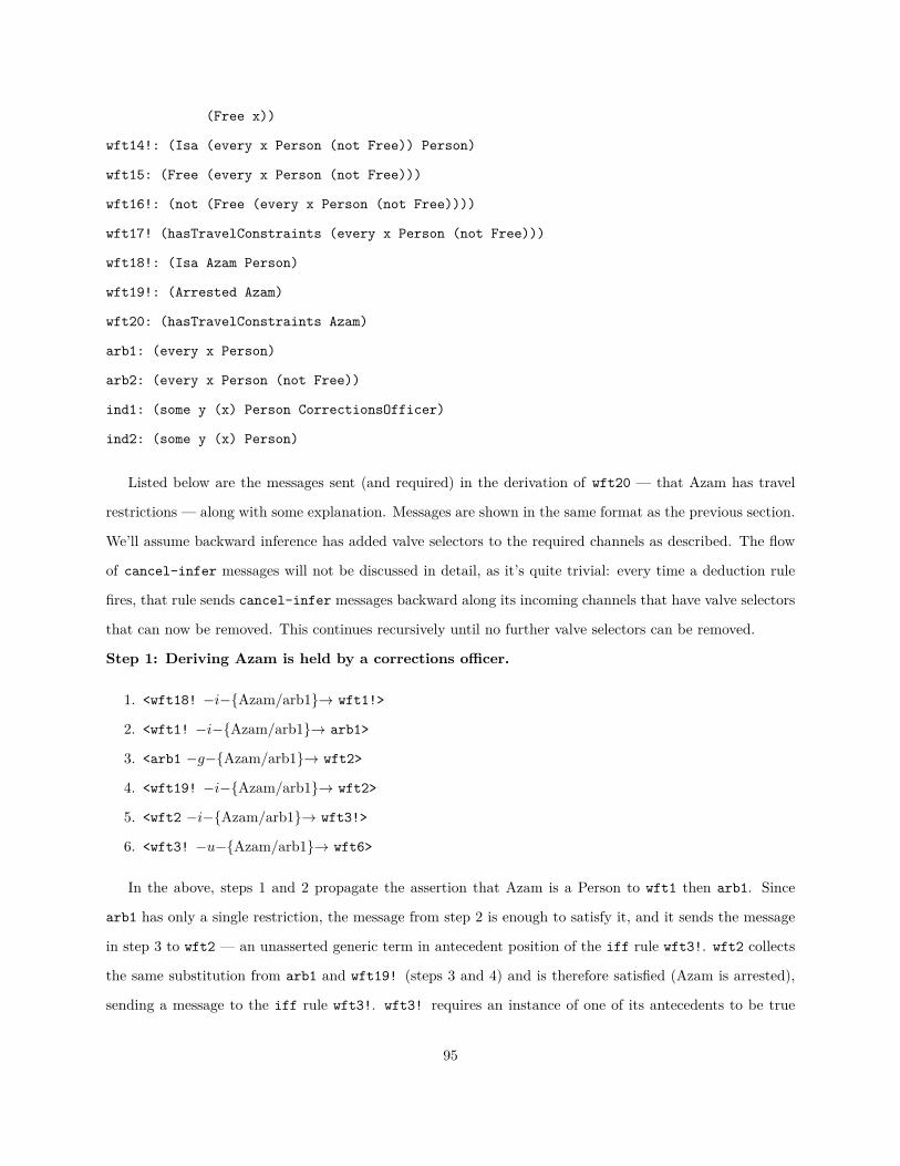
(Free x))
wft14!: (Isa (every x Person (not Free)) Person)
wft15: (Free (every x Person (not Free)))
wft16!: (not (Free (every x Person (not Free))))
wft17! (hasTravelConstraints (every x Person (not Free)))
wft18!: (Isa Azam Person)
wft19!: (Arrested Azam)
wft20: (hasTravelConstraints Azam)
arb1: (every x Person)
arb2: (every x Person (not Free))
ind1: (some y (x) Person CorrectionsOfficer)
ind2: (some y (x) Person)
Listed below are the messages sent (and required) in the derivation of wft20 — that Azam has travel
restrictions — along with some explanation. Messages are shown in the same format as the previous section.
We’ll assume backward inference has added valve selectors to the required channels as described. The flow
of cancel-infer messages will not be discussed in detail, as it’s quite trivial: every time a deduction rule
fires, that rule sends cancel-infer messages backward along its incoming channels that have valve selectors
that can now be removed. This continues recursively until no further valve selectors can be removed.
Step 1: Deriving Azam is held by a corrections officer.
1. <wft18! −i−{Azam/arb1}→ wft1!>
2. <wft1! −i−{Azam/arb1}→ arb1>
3. <arb1 −g−{Azam/arb1}→ wft2>
4. <wft19! −i−{Azam/arb1}→ wft2>
5. <wft2 −i−{Azam/arb1}→ wft3!>
6. <wft3! −u−{Azam/arb1}→ wft6>
In the above, steps 1 and 2 propagate the assertion that Azam is a Person to wft1 then arb1. Since
arb1 has only a single restriction, the message from step 2 is enough to satisfy it, and it sends the message
in step 3 to wft2 — an unasserted generic term in antecedent position of the iff rule wft3!. wft2 collects
the same substitution from arb1 and wft19! (steps 3 and 4) and is therefore satisfied (Azam is arrested),
sending a message to the iff rule wft3!. wft3! requires an instance of one of its antecedents to be true
95

for its consequents to be true, so it sends a message to wft6, indicating that an instance of wft6 is derived
with the given substitution. This instance indicates Azam is held by a corrections officer.
Step 2: Deriving Azam is detained.
1. <wft6 −i−{Azam/arb1, ind1/ind2}→ wft9>
2. <arb1 −g−{Azam/arb1}→ ind2>
3. <ind2 −g−{Azam/arb1, ind3/ind2}→ wft9>
4. <wft9 −i−{Azam/arb1}→ wft10!>
5. <wft10! −u−{Azam/arb1}→ wft7>
Since persons who are corrections officers are persons, wft6 relays its substitution to wft9. wft9 collects
compatible instances from wft6 and ind2. Note that ind2 creates ind3: (some x () (Isa x Person)
(notSame x Azam)), in step 3. These compatible substitutions satisfy wft9 — that Azam is held by a
person — allowing for iff-elimination in steps 4 and 5, deriving that Azam is detained.
Step 3: Deriving Azam is not free.
1. <wft7 −i−{Azam/arb1}→ wft13!>
2. <wft13! −u−{Azam/arb1}(neg)→ wft12>
Since an instance of wft7 was found, its substitution is sent to wft13! for xor-elimination — producing
the negation of wft12 with the substitution {Azam/arb1} in step 2. So, Azam is not free.
Step 4: Deriving Azam has travel restrictions.
1. <wft18! −i−{Azam/arb2}→ wft14!>
2. <wft14! −i−{Azam/arb2}→ arb2>
3. <wft12 −i−{Azam/arb2}(neg)→ wft15>
4. <wft15 −i−{Azam/arb2}(neg)→ wft16!>
5. <wft16! −i−{Azam/arb2}→ arb2>
6. <arb2 −g−{Azam/arb2}→ wft17!>
7. <wft17! −i−{}→ wft20>
Since Azam is a person, Azam satisfies one of the restrictions of arb2, as determined in steps 1 and
2. Azam is not free, as found previously, so steps 3-5 recognize that Azam satisfies the second restriction
96
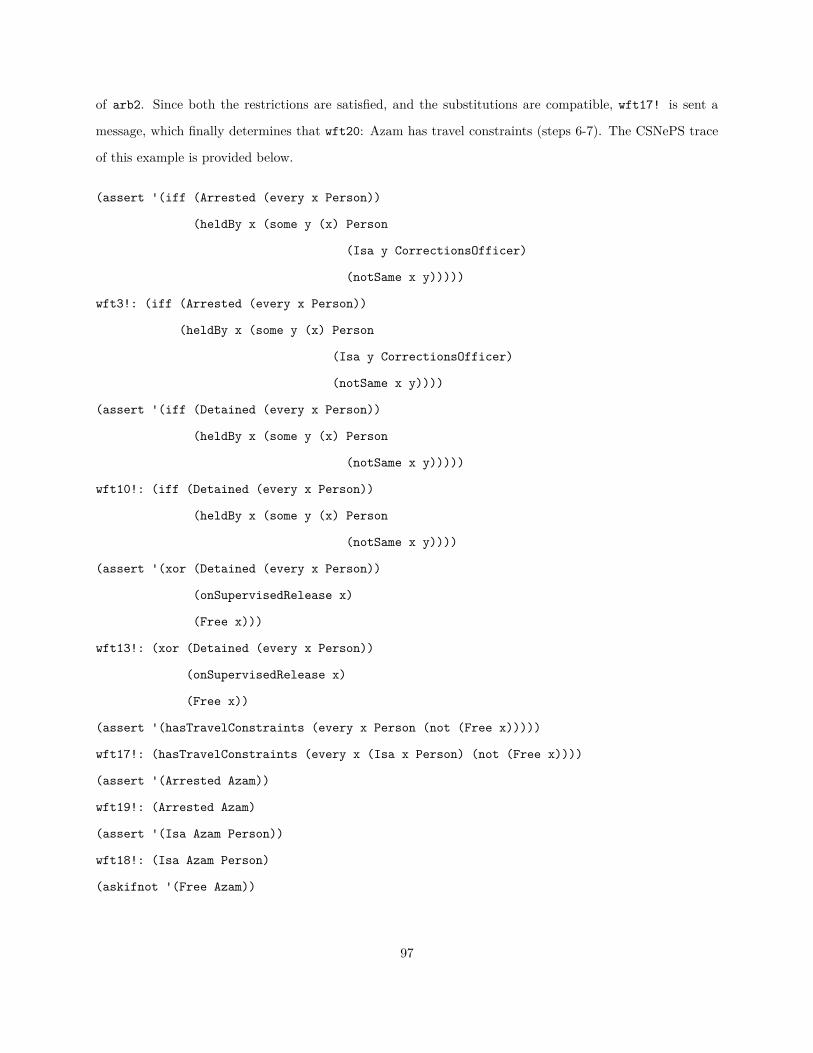
of arb2. Since both the restrictions are satisfied, and the substitutions are compatible, wft17! is sent a
message, which finally determines that wft20: Azam has travel constraints (steps 6-7). The CSNePS trace
of this example is provided below.
(assert '(iff (Arrested (every x Person))
(heldBy x (some y (x) Person
(Isa y CorrectionsOfficer)
(notSame x y)))))
wft3!: (iff (Arrested (every x Person))
(heldBy x (some y (x) Person
(Isa y CorrectionsOfficer)
(notSame x y))))
(assert '(iff (Detained (every x Person))
(heldBy x (some y (x) Person
(notSame x y)))))
wft10!: (iff (Detained (every x Person))
(heldBy x (some y (x) Person
(notSame x y))))
(assert '(xor (Detained (every x Person))
(onSupervisedRelease x)
(Free x)))
wft13!: (xor (Detained (every x Person))
(onSupervisedRelease x)
(Free x))
(assert '(hasTravelConstraints (every x Person (not (Free x)))))
wft17!: (hasTravelConstraints (every x (Isa x Person) (not (Free x))))
(assert '(Arrested Azam))
wft19!: (Arrested Azam)
(assert '(Isa Azam Person))
wft18!: (Isa Azam Person)
(askifnot '(Free Azam))
97

Since: wft3!: (iff (Arrested (every x Person))
(heldBy x (some y (x) Person
(Isa y CorrectionsOfficer)
(notSame x y)))))
and: wft19!: (Arrested Azam)
and: wft18!: (Isa Azam Person)
I derived: wft24!: (heldBy Azam (some y () (Isa y Person)
(Isa y CorrectionsOfficer)
(notSame y Azam))) by iff-elimination
Since: wft10!: (iff (Detained (every x (Isa x Person)))
(heldBy x (some y (x) (Isa y Person) (notSame y x))))
and: wft24!: (heldBy Azam (some y () (Isa y Person)
(Isa y CorrectionsOfficer)
(notSame y Azam)))
I derived: wft25!: (Detained Azam) by iff-elimination
Since: wft13!: (xor (Detained (every x (Isa x Person))) (onSupervisedRelease x) (Free x))
and: wft25!: (Detained Azam)
and: wft18!: (Isa Azam Person)
I derived: wft21!: (not (Free Azam)) by xor-elimination
6.4.3 Bi-directional Inference and Focused Reasoning3
Bi-directional inference involves the combination of forward and backward inference procedures. Since the
concepts are so closely related, it is best to combine the discussion of bi-directional inference with the
discussion of focused reasoning.
Three types of focused reasoning are possible within a reasoning system: (1) focused forward reasoning,
where all possible derivations are performed only from some specific new piece of knowledge, and continued
upon the addition of relevant rules to the KB; (2) forward-in-backward focused reasoning, in which backward
inference occurs to try to answer a query, and as new facts or rules relevant to the query are added to the3This section is adapted from (Schlegel and Shapiro, 2014b)
98

KB, they are used in attempting to answer the query; and (3) backward-in-forward focused reasoning, which
combines the previous two focused reasoning mechanisms.
Focused forward reasoning can be thought of as a kind of full-forward reasoning carried out only for
a single asserted term. Full-forward reasoning is used most notably in production systems, and especially
RETE networks. In a RETE net, all new information is filtered through a graph generated from a set of
production rules. Nodes in the graph perform comparisons against accepted values, and combine pieces of
compatible information together. When a piece of information reaches some leaf node in the graph, the rule
that that leaf node represents is said to have matched. Full-forward inference produces the logical closure of
a KB, but this is horribly wasteful in both time and space, so we favor doing this only when it’s explicitly
asked for. In addition, RETE nets are limited — no new rules can be added once the system is started,
which is not the case with IGs.
For reasoning systems capable of backward and bi-directional reasoning, the issue of focused reasoning is
seldom tackled. SNePS 2’s ACG has a concept of “activating” a path of nodes when backward inference does
not result in an answer. Later assertions meant to use this path must be asserted with forward inference
(that is that term is asserted, and forward inference is carried out for that term only), and that forward
inference process will use activated paths exclusively whenever they are available (Shapiro et al., 1982). The
ACG is unable to later deactivate the path of nodes, so the conflation of the specialized forward inference
using activated paths with the usual forward inference that ignores activated paths results in the need to
occasionally throw the graph away as it could interfere with future inference tasks. In addition, activated
paths are not extended backward when rules relevant to the reasoning task are added to the KB.
Inference Graphs are capable of performing forward, forward-in-backward, and backward-in-forward fo-
cused reasoning. They also allow the addition of new rules once the system is running, extending the focused
region of the graph. In addition, they do not limit the functionality of the graph in other ways — other
inference tasks can be performed as usual. In effect, our system has none of the limitations of RETE nets,
or ACGs, while being more a more powerful, focused, reasoning tool.
6.4.3.1 Forward-In-Backward Focused Reasoning
The most common use of focused reasoning is when wondering about something that cannot yet be answered
by the system using backward inference. For example, consider a knowledge base containing only (if P R)
and (if P Q). Then, the user asks about R. Backward inference is set up (i.e., valves in the appropriate
channels through (if P R) are opened) but no answer is forthcoming. Later, P is asserted (without forward
99

inference). Since the appropriate valves are already open, R is derived immediately, without needing to pose
the question again. Note that Q is not derived, since valves involving (if P Q) were not opened during
backward inference.4
In a somewhat more complex example from the counter-insurgence domain, consider the following initial
knowledge base:
;; Azam is a person
(Isa Azam Person)
;; If a person is arrested, they are detained.
(if (Arrested (every x Person))
(Detained x))
;; A person is either detained or free.
(xor (Detained (every x Person))
(Free x))
It is then asked by a user, “who are the detained persons?”: (Detained (?x (Isa ?x Person)). The top
graph in Figure 6.3 shows the IG for this KB. The complete listing of terms in this graph are given below.
wft1: (Arrested (every x Person))
wft2: (Detained (every x Person))
wft3!: (if (Arrested (every x Person)) (Detained x))
wft4: (Free (every x Person))
wft5!: (xor (Detained (every x Person)) (Free x))
wft6!: (Arrested Azam)
wft8!: (Isa (every x Person) Person)
wft9!: (Isa Azam Person)
wft12!: (Isa (?x Person) Person)
wft20: (Detained (?x Person))
arb1: (every x Person)4Prolog with tabling can suspend some paths of inference that cannot complete, and resume them if useful facts are added
using a special function (Swift and Warren, 2012). Focused reasoning is better, allowing automatic continuation of inferenceat the time when related terms are added to the KB in the normal way, and always persisting beyond the run time of a singleinference procedure.
100
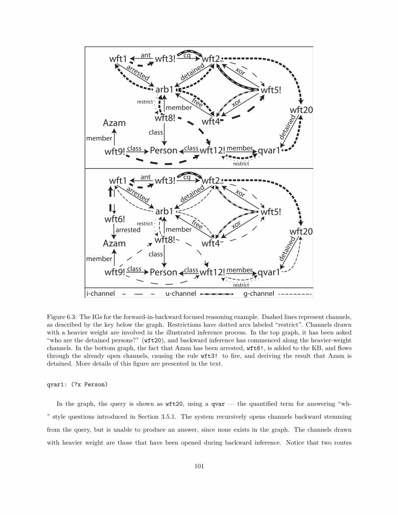
arb1
wft1 wft3! wft2ant cqarrested det
ained
wft4
free
wft5!
xor
xor
qvar1
wft20
detained
Person
wft8!
restrictmember
class
wft12!memberclass
restrict
Azam
wft6!arrested
wft9!member
class
arb1
wft1 wft3! wft2ant cqarrested det
ained
wft4
free
wft5!
xor
xor
qvar1Person
wft8!
restrictmember
class
wft12!memberclass
restrict
Azam
wft9!member
class
wft20
detained
i-channel u-channel g-channel
Figure 6.3: The IGs for the forward-in-backward focused reasoning example. Dashed lines represent channels,as described by the key below the graph. Restrictions have dotted arcs labeled “restrict”. Channels drawnwith a heavier weight are involved in the illustrated inference process. In the top graph, it has been asked“who are the detained persons?” (wft20), and backward inference has commenced along the heavier-weightchannels. In the bottom graph, the fact that Azam has been arrested, wft6!, is added to the KB, and flowsthrough the already open channels, causing the rule wft3! to fire, and deriving the result that Azam isdetained. More details of this figure are presented in the text.
qvar1: (?x Person)
In the graph, the query is shown as wft20, using a qvar — the quantified term for answering “wh-
” style questions introduced in Section 3.5.1. The system recursively opens channels backward stemming
from the query, but is unable to produce an answer, since none exists in the graph. The channels drawn
with heavier weight are those that have been opened during backward inference. Notice that two routes
101

are tried — A person might be detained if they are not free, or a person might be detained if they have
been arrested. At some later time, it is added to the KB that Azam was arrested: (Arrested Azam). The
system knows that backward inference was in progress,5 so upon the addition of the channel from wft6! to
wft1, backward inference is continued back to wft6!, opening that channel. Since wft6! is asserted, this
information immediately flows forward through the graph along open channels, and Azam is produced as an
answer to the previously added query automatically. This is shown in the bottom half of Figure 6.3, where
the heavier weight channels indicate the flow of messages from wft6! forward through the open channels.
It’s important to note that while this KB entails that Azam is not free, it does not derive this fact in this
case since the channels from wft2 to wft5! and wft5! to wft4 were not opened by the backward inference
process. So, derivations that are irrelevant to reaching the desired conclusion are not performed — we say
inference is focused toward the query.
As expected, CSNePS performs this inference using IGs accordingly, as in the below inference trace.
(assert '(Isa Azam Person))
wft9!: (Isa Azam Person)
(assert '(if (Arrested (every x (Isa x Person))) (Detained x)))
wft3!: (if (Arrested (every x (Isa x Person))) (Detained x))
(assert '(xor (Detained (every x (Isa x Person))) (Free x)))
wft5!: (xor (Free (every x (Isa x Person))) (Detained x))
(askwh '(Detained (?x (Isa ?x Person))))
nil
(assert '(Arrested Azam))
wft6!: (Arrested Azam)
Since wft3!: (if (Arrested (every x (Isa x Person))) (Detained x))
and wft9!: (Isa Azam Person)
and wft6!: (Arrested Azam)
I derived: wft11!: (Detained Azam) by implication-elimination5How does it know? In many cases, it is possible to tell by which channels are open. But, there are cases where this doesn’t
work (such as initiating backward inference on a term with no incoming channels), so it makes more sense to maintain a set ofin-progress processes or a flag as detailed later.
102

6.4.3.2 Forward Focused Reasoning
A second type of focused reasoning can occur when a user wishes to perform forward inference on a term,
but the knowledge base is not yet fully constructed. For example, consider an empty knowledge base where
the user asserts Q with forward inference. Nothing new is derived, as the KB is otherwise empty. Later,
(if Q R) is asserted. Since Q was asserted with forward inference, as soon as additional outgoing channels
are connected to it, its assertional status flows forward through the graph, and R is derived. This derivation
happens, again, without needing to reassert Q. One can think about this as a limited form of full-forward
inference. Instead of adopting full-forward inference for all terms that are added to the KB, only Q has this
property. Automatic inference in the graph is focused on what can be derived from Q, while unrelated terms
(e.g., (if S T) and S) may be added but without resulting in any automatic inference.
It’s worth recognizing that all our inference mechanisms only follow existing channels, and do not create
new terms that are possibly irrelevant to the knowledge base. For example, from the original KB with only
Q asserted, there are an infinite number of true disjunctions that could be introduced, but are unhelpful for
ongoing inference processes.
Consider our counter-insurgence example again with a slightly different set of terms initially asserted:
;; A person is either detained or free.
(xor (Detained (every x Person))
(Free x))
It is then asserted with forward inference that Azam is a person, and has been arrested: (Isa Azam Person),
and (Arrested Azam). The top of Figure 6.4 shows the resulting knowledge base. It is determined that
Azam satisfies the restriction of arb1 (that is, Azam is a Person, through the channel from wft9! to wft8!),
but no new knowledge is derived. Later, as in the bottom of Figure 6.4, the rule that if a person is arrested
then they have been detained is added:
(if (Arrested (every x Person))
(Detained x))
Since wft6! was added with forward inference, when the new outgoing channel to wft1 is added, forward
inference continues. This allows the derivations that Azam is detained: (Detained Azam), and Azam is not
free: (not (Free Azam)).
The complete listing of terms used in Figure 6.4 are provided below.
103
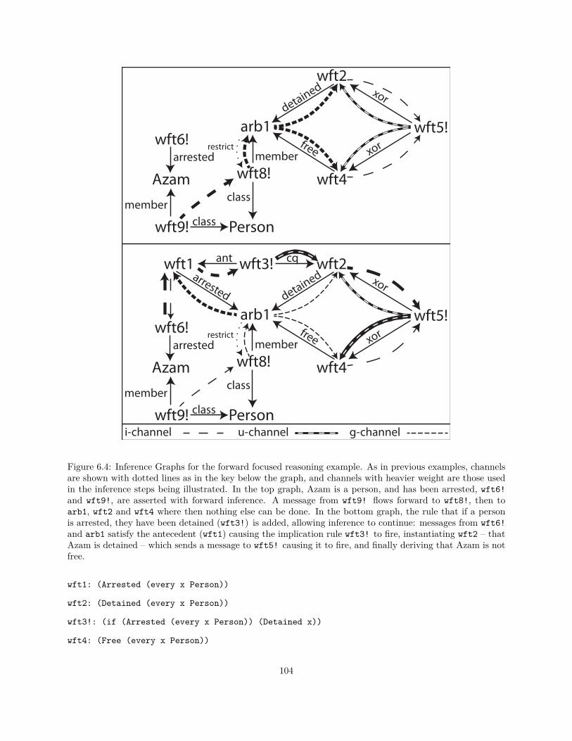
arb1
wft2
detain
ed
wft4
free
wft5!
xor
xor
Azam
wft6!arrested
Person
wft8!
restrictmember
class
wft9!member
class
arb1
wft1 wft3! wft2ant cqarrested det
ained
wft4
free
wft5!
xor
xor
Azam
wft6!arrested
Person
wft8!
restrictmember
class
wft9!member
class
i-channel u-channel g-channel
Figure 6.4: Inference Graphs for the forward focused reasoning example. As in previous examples, channelsare shown with dotted lines as in the key below the graph, and channels with heavier weight are those usedin the inference steps being illustrated. In the top graph, Azam is a person, and has been arrested, wft6!and wft9!, are asserted with forward inference. A message from wft9! flows forward to wft8!, then toarb1, wft2 and wft4 where then nothing else can be done. In the bottom graph, the rule that if a personis arrested, they have been detained (wft3!) is added, allowing inference to continue: messages from wft6!and arb1 satisfy the antecedent (wft1) causing the implication rule wft3! to fire, instantiating wft2 – thatAzam is detained – which sends a message to wft5! causing it to fire, and finally deriving that Azam is notfree.
wft1: (Arrested (every x Person))
wft2: (Detained (every x Person))
wft3!: (if (Arrested (every x Person)) (Detained x))
wft4: (Free (every x Person))
104

wft5!: (xor (Detained (every x Person)) (Free x))
wft6!: (Arrested Azam)
wft8!: (Isa (every x Person) Person)
wft9!: (Isa Azam Person)
arb1: (every x Person)
As expected, CSNePS performs this inference task similarly, as shown below.
(assert '(xor (Detained (every x (Isa x Person))) (Free x)))
wft5!: (xor (Free (every x (Isa x Person))) (Detained x))
(assert! '(Isa Azam Person))
wft9!: (Isa Azam Person)
(assert! '(Arrested Azam))
wft6!: (Arrested Azam)
(assert '(if (Arrested (every x (Isa x Person))) (Detained x)))
wft3: (if (Arrested (every x (Isa x Person))) (Detained x))
Since: wft3!: (if (Arrested (every x (Isa x Person))) (Detained x))
and: wft9!: (Isa Azam Person)
and: wft6!: (Arrested Azam)
I derived: wft10!: (Detained Azam) by if-elimination
Since: wft5!: (xor (Free (every x (Isa x Person))) (Detained x))
and: wft10!: (Detained Azam)
and: wft9!: (Isa Azam Person)
I derived: wft11!: (not (Free Azam)) by xor-elimination
6.4.3.3 Backward-In-Forward Focused Reasoning
A combination of the above two focused reasoning techniques is also possible. Consider a user who again
asserts Q with forward inference into an empty knowledge base. Later, (if P (if Q R)) is asserted. As with
forward focused reasoning, Q recognizes that it has new outgoing channels, and sends its assertional status
to (if Q R). But, (if Q R) is not yet asserted, so backward inference attempts to derive (if Q R), but
105

fails. Later again, P is asserted (without forward inference). Inference then occurs as in forward-in-backward
focused reasoning, (if Q R) is derived, then R is.
From the counter-insurgence domain again, consider the KB:
;; Ahmad is a person.
(Isa Ahmad Person)
;; If a person is a person of interest (POI),
;; they are either under surveillance, or being sought out.
(if (POI (every x Person))
(xor (UnderSurveillance x)
(BeingSoughtOut x)))
;; If a person is a POI, they are of interest to INSCOM
(if (POI (every x Person))
(ofInterestTo x INSCOM))
Now, it is asserted with forward inference that Ahmad is not under surveillance: (not (UnderSurveillance
Ahmad)), shown in the top of Figure 6.5. If the xor (wft5) were asserted, it could be derived that
(BeingSoughtOut Ahmad) through forward inference, but it is not. So, the system initiates backward infer-
ence to attempt to derive the xor, by checking whether Ahmad is a POI. Since the system has no answer
for that, inference halts. Sometime later, shown in the bottom half of Figure 6.5, (POI Ahmad) is added to
the KB. The xor receives a message saying it is able to be used for the substitution of Ahmad for arb1 (but
not in general), and the initial forward inference task resumes, deriving (BeingSoughtOut Ahmad). Here
again it’s worth noting that even though the IG entails that Ahmad is of interest to INSCOM, that was
not derived since it was of no use to the backward inference task attempting to derive wft5, and it does
not follow directly from the fact that Ahmad is not under surveillance, which was the assertion made with
forward inference.
To assist in understanding the figure, each term used is listed below.
wft1: (POI (every x Person))
wft2: (UnderSurveillance (every x Person))
wft3!: (if (POI (every x Person))
106

(xor (UnderSurveillance x) (BeingSoughtOut x)))
wft4: (BeingSoughtOut (every x Person))
wft5: (xor (UnderSurveillance x) (BeingSoughtOut x))
wft8!: (Isa (every x Person) Person)
wft9!: (Isa Ahmad Person)
wft13: (UnderSurveillance Ahmad)
wft14!: (not (UnderSurveillance Ahmad))
wft15!: (POI Ahmad)
wft16!: (if (POI (every x Person)) (ofInterestTo x INSCOM))
wft17: (ofInterestTo (every x Person) INSCOM)
arb1: (every x Person)
As expected, CSNePS performs this inference task as described.
(assert '(Isa Ahmad Person))
wft9!: (Isa Ahmad Person)
(assert '(if (POI (every x (Isa x Person)))
(xor (UnderSurveillance x) (BeingSoughtOut x))))
wft3!: (if (POI (every x (Isa x Person)))
(xor (UnderSurveillance x) (BeingSoughtOut x)))
(assert '(if (POI (every x (Isa x Person))) (ofInterestTo x INSCOM)))
wft16!: (if (POI (every x (Isa x Person))) (ofInterestTo x INSCOM))
(assert! '(not (UnderSurveillance Ahmad)))
wft14!: (not (UnderSurveillance Ahmad))
(assert '(POI Ahmad))
wft15!: (POI Ahmad)
Since: wft3!: (if (POI (every x (Isa x Person)))
(xor (UnderSurveillance x) (BeingSoughtOut x)))
and: wft15!: (POI Ahmad)
and: wft9!: (Isa Ahmad Person)
I derived: wft18!: (xor (BeingSoughtOut Ahmad)
107

(UnderSurveillance Ahmad)) by if-elimination
Since: wft18!: (xor (BeingSoughtOut Ahmad) (UnderSurveillance Ahmad))
and: wft14!: (not (UnderSurveillance Ahmad))
I derived: wft19!: (BeingSoughtOut Ahmad) by xor-elimination
6.4.3.4 A Unifying Algorithm
In order to perform focused reasoning using IGs, two requirements must be fulfilled. Nodes must track
whether they are part of a focused reasoning task (which one, and in which direction(s)), and whenever a
channel is added to the graph it must be determined if forward or backward inference must continue along
that channel.
Focused reasoning makes use of two sets, initially empty, which are part of every node: fBR for focused
inference tasks requiring future backward reasoning at that node, and fFwR for focused inference tasks
requiring future forward reasoning at that node. As backward-infer messages propagate backward through
the graph adding valve selectors channels, they add the goal of the backward reasoning task to the fBR
set in each node. When forward inference is initiated, nodes reached have their fFwR set augmented with
the origin of the forward inference task. backward-infer messages are allowed to travel backward along
already channels that already have appropriate valve selectors if these sets need to be updated. Tracking
which nodes are involved in each type of focused inference task allows one focused inference task to later be
canceled without affecting the others.6 To cancel these tasks, cancel-infer messages are used, which will
only remove a valve selector if it’s not needed for any more focused inference tasks, but can travel backward
though the graph removing an entry from the nodes sets of future inference tasks.
When a new channel is added to the graph, the contents of its origin’s fFwR or destination’s fBR set
determine whether or not to continue a focused reasoning task. If a new channel is created, and its origin’s
fFwR set is non-empty, forward inference is continued along that new channel (and recursively forward), and
the contents of the fFwR set is propagated forward. If a new channel has a destination with a non-empty
fBR set, then backward inference starts at the new channel (and continues recursively), and the contents
of the fBR set is propagated backward. These routines combine to allow for forward-in-backward focused6If one wanted to simply cancel all or no focused reasoning tasks, these sets could be replaced with flags. Some book keeping
is still required since it is impossible to tell whether forward or backward inference has been initiated from a node otherwisedisconnected from the graph without some marker.
108

reasoning, and forward focused reasoning.
The final aspect of the algorithm occurs when a rule is not asserted, but receives an i-infer message
via forward inference, indicating an attempt to use that rule. In this case, that node attempts to have itself
derived in general or for a specific substitution by beginning a backward reasoning task, adding itself to it’s
fBR set, and propagating that set backward. Once the rule has been derived, it recursively sends messages
canceling the backward reasoning task backward through the graph, since it’s purpose has been fulfilled.
This allows for backward-in-forward focused reasoning.
Where a human probably has some limit to the number of these types of tasks they can perform, we
impose no such limits. An interesting future task may be to use this alongside an agent who has a finite
number of tasks they can work on, and is “forgetful.”
6.5 Message Processing Algorithm
In order to make it more clear what happens when a message arrives at a node, Algorithm 6.1 is presented.
This algorithm decides when introduction and elimination rules are to be attempted. It also handles several
parts of the focused reasoning algorithm — determining when to invoke backward-in-forward inference, for
example.
109

Algorithm 6.1 The algorithm for processing an inference message. This algorithm determineswhen introduction or elimination rules should be attempted. The functions attemptElimination andattemptIntroduceOrInstantiate dispatch on the type of node and attempt to satisfy the implementedinference rules (in which case, more messages are sent). applySubst applies a substitution to a term(node). minimalUnion produces a union of support sets, where every included origin set is minimal.submitToChannel sends a message on a particular channel.function processMessage(msg, node)
if fwd?msg thenfFwRnode ← fFwRnode ∪ fFwRoriginmsg
end ifif typemsg = i-infer then . Attempt elimination.
attemptEliminate(msg, node)else if typemsg = u-infer then . u-infer instantiates a term as true/false.
term← nilif true?msg then
term← applySubst(node, substmsg)attemptEliminate(msg, node)
elseterm← applySubst((not node), substmsg)
end ifsupportterm ← minimalUnion(supportterm, supportmsg)newmsg ← msgoriginnewmsg ← termsupportnewmsg ← supporttermtypenewmsg ← i-inferfor all ch ∈ ichnode do . Tell i-channel attached nodes of the new instance.
submitToChannel(ch, newmsg)end forif term ∈ fBRnode then . Cancel completed Forward-In-Backward Focused Reasoning.
cancelInferOf(node)end if
end ifif typemsg = i-infer or typemsg = g-infer then . Attempt introduction/instantiation.
if analytic ∈ propertiesnode then . Don’t instantiate analytic terms.for all ch ∈ gchnode do
submitToChannel(ch, msg)end for
elseresult← attemptIntroduceOrInstantiate(msg, node)if fwd?msg and empty?(result) then . Do Backward-In-Forward Focused Reasoning
backwardInfer(node)end if
end ifend if
end function
110
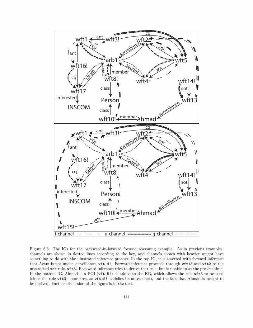
arb1
wft1 wft3! wft2antcq
survei
llance
wft4
sought
wft5
xor
xor
Ahmad
Person
wft8!restric
t
member
class
wft10!class
member
POI
wft13
survei
llance
wft14!not
arb1
wft1 wft3! wft2antcq
survei
llance
wft4
sought
wft5
xor
xor
Ahmad
Person
wft8!
restric
t
member
class
wft10!class
member
POI
wft13
survei
llance
wft14!not
wft15!POI
wft16!
wft17
ant
cq
INSCOM
interested
target
wft16!
wft17
ant
cq
INSCOM
interested
target
i-channel u-channel g-channel
Figure 6.5: The IGs for the backward-in-forward focused reasoning example. As in previous examples,channels are shown in dotted lines according to the key, and channels shown with heavier weight havesomething to do with the illustrated inference process. In the top IG, it is asserted with forward inferencethat Azam is not under surveillance, wft14!. Forward inference proceeds through wft13 and wft2 to theunasserted xor rule, wft5. Backward inference tries to derive that rule, but is unable to at the present time.In the bottom IG, Ahmad is a POI (wft15!) is added to the KB, which allows the rule wft5 to be used(since the rule wft3! now fires, as wft15! satisfies its antecedent), and the fact that Ahmad is sought tobe derived. Further discussion of the figure is in the text.
111

Chapter 7
Concurrency and Scheduling
Heuristics
The structure of IGs lends itself naturally to concurrent inference. Every example seen throughout this
dissertation has had situations where multiple paths (made up of channels) could be examined simultaneously.
Any number of nodes in the graph may process messages simultaneously without fear of interfering with any
others. Only when a single node receives multiple messages must those messages be processed synchronously.
This synchronous processing is necessary because the message caches are shared state. We need not concern
ourselves with the actual order in which the messages are processed, since the operation is commutative,
meaning there is no need to maintain a queue of changes to the message cache.
In Section 7.1 the basic approach toward concurrency taken by IGs is presented. Section 7.2 discusses
the scheduling heuristics that have been devised to ensure that concurrent processing is done as efficiently
as possible. The issue of multiple inference processes is discussed in Section 7.3. Evaluation of concurrency
characteristics are presented in Section 7.4.
7.1 Concurrency
In Chapter 2, approaches to concurrency in theorem proving systems which used different granularities of
concurrency were presented. That work found that the best performing granularity was the sub-goal level.
In IGs, this translates to concurrency at the node level.
In order to perform inference concurrently, the inference graph is divided into inference segments (hence-
112

forth, segments). A segment represents the inference operation — from receipt of a message to sending new
ones — which occurs in a node. Valves delimit segments, as seen in Figure 7.1. When a message passes
through a valve a new task is created — the application of the segment’s inference function to the message.
When tasks are created they enter a global prioritized queue, where the priority of the task is the priority of
the message. When the task is executed, inference is performed as described in previous chapters, and any
newly generated messages are sent toward its outgoing valves for the process to repeat.
wft1!Filter Switch Valve
... ...Valve
Inference Segment
Figure 7.1: A single inference segment is shown in the gray bounding box.
7.2 Scheduling Heuristics
The goal of any inference system is to infer the knowledge requested by the user. If we arrange an inference
graph so that a user’s request (in backward inference) is on the right, and channels flow from left to right
wherever possible (the graph may contain cycles), we can see this goal as trying to get messages from the
left side of the graph to the right side of the graph. We, of course, want to do this as quickly as possible.
Every inference operation begins processing inference messages some number of levels to the left of
the query node. Since there are a limited number of tasks that can be running at once due to hardware
limitations, we must prioritize their execution, remove tasks that we know are no longer necessary, and
prevent the creation of unnecessary tasks. Therefore,
1. tasks for relaying newly derived information using segments to the right are executed before those to
the left,
2. once a node is known to be true or false, all tasks still attempting to derive it are canceled, as long
as their results are not needed elsewhere, and in all channels pointing to it that may still derive it,
appropriate valve selectors are removed, and
113
3. once a rule fires, all tasks for potential antecedents of that rule still attempting to satisfy it are canceled,
as long as their results are not needed elsewhere, and in all channels from antecedents that may still
satisfy it, appropriate valve selectors are removed.
Together, these three heuristics ensure that messages reach the query as quickly as possible, and time
is not wasted deriving unnecessary formulas (though, as mentioned earlier, it may prevent the automatic
derivation of contradictions). The priorities of the messages (and hence, tasks) allow us to reach these
goals. All cancel-infer messages have the highest priority. Then come i-infer and u-infer messages.
backward-infer messages have the lowest priority. As i-infer and u-infer messages flow to the right,
they get higher priority, but their priorities remain lower than that of cancel-infer messages. In forward
inference, i-infer and u-infer messages to the right in the graph always have higher priority than those
to the left, since the messages all begin flowing from a common point. In backward inference, the priorities
of backward-infer, i-infer, and u-infer messages work together to derive a query formula as quickly as
possible. Since backward-infer messages are of the lowest priority, those i-infer and u-infer messages
waiting at valves that are nearest to the query formula begin flowing forward before valve sectors further
away are added. This, combined with the increasing priority of i-infer and u-infer messages ensure
efficient derivation. In short, the closest possible path to the query formula is always attempted first in
backward inference.
The design of the system therefore ensures that the tasks executing at any time are the ones closest to
deriving the goal, and tasks that will not result in useful information towards deriving the goal are cleaned
up. Additionally, since nodes “push” messages forward through the graph instead of “pulling” from other
nodes, it is not possible to have tasks running waiting for the results of other rule nodes’ tasks. Thus,
deadlocks are impossible, and bottlenecks can only occur when multiple threads are making additions to
shared state simultaneously.
7.2.1 Example
Inspired by L. Frank Baum’s The Wonderful Wizard of Oz (Baum, 1900), we consider a scene in which
Dorothy and her friends are being chased by Kalidas — monsters with the head of a tiger and the body of
a bear. In the world of Oz, whenever a dog becomes scared, the owner of the dog carries it, and that’s the
only time the dog is carried. If a dog is carried, it does not walk, and if it walks, it is not carried. Toto, a
dog, becomes scared when Dorothy, Toto’s owner, is being chased. Since Dorothy has only two hands, she is
capable of either carrying the Scarecrow (who is large, and requires both hands), or between 1 and 2 of the
114

following items: Toto, her full basket, and the Tin Woodman’s oil can. In our example, the Tin Woodman
is carrying his own oil can. Only one of Dorothy, the Scarecrow, or the Tin Woodman can carry the oil can
at once. The relevant parts of this scene are represented below in their logical forms.1
;;; Dorothy is a person, Toto is a dog, and Dorothy owns Toto.
(Isa Dorothy Person)
(Isa Toto Dog)
(Owns Dorothy Toto)
;;; Dorothy can either carry the scarecrow,
;;; or carry one or two objects from the list:
;;; her full basket, Toto, oil can.
(xor (Carries Dorothy Scarecrow)
(andor (1 2) (Carries Dorothy FullBasket)
(Carries Dorothy Toto)
(Carries Dorothy OilCan)))
;;; Either Dorothy, the Tin Woodman, or the Scarecrow carry the Oil Can.
(xor (Carries Dorothy OilCan)
(Carries TinWoodman OilCan)
(Carries Scarecrow OilCan))
;;; Either someone carries a dog, or the dog walks.
(assert '(xor (Walks (every y (Isa y Dog)))
(close x (Carries (some x (y) (Isa x Person))
y))))
;;; A dog is carried by its owner, if and only if the dog is scared.1Representing the owner of a dog in “a dog is carried by its owner” is difficult given the implemented logic. It is not
appropriate to make use of an indefinite term to represent the owner, since we would like to derive that Dorothy is the one whocarries Toto (after all, Dorothy is the owner of Toto). Using an arbitrary term also seems odd — what would it mean for a dogto be carried by more than one person, if it had more than one owner? What would be best would be a quantified term whichrepresents the definite description of a person — that is, there would be one and only one satisfier of such a quantified term.Implementing such a quantified term is an item of future work (see Section 9.2.2.2).
115

(iff (Scare (every x Dog)) (Carries (every y Person (Owns x)) x))
;;; Toto gets scared if Dorothy is being chased.
(if (Chase Dorothy) (Scare Toto))
;;; The Tin Woodman is carrying his Oil Can.
(Carries TinWoodman OilCan)
;;; Dorothy is being chased.
(Chase Dorothy)
We can then wonder, “Is Dorothy carrying the Scarecrow?" According to the rules of inference, it is
derivable that this is not the case. CSNePS is able to derive this as follows:2
(assert '(Isa Dorothy Person))
wft20!: (Isa Dorothy Person)
(assert '(Isa Toto Dog))
wft16!: (Isa Toto Dog)
(assert '(Owns Dorothy Toto))
wft15!: (Owns Dorothy Toto)
(assert '(xor (Carries Dorothy Scarecrow)
(andor (1 2) (Carries Dorothy FullBasket)
(Carries Dorothy Toto)
(Carries Dorothy OilCan))))
wft6!: (xor (Carries Dorothy Scarecrow)
(andor (1 2) (Carries Dorothy FullBasket)
(Carries Dorothy Toto)
(Carries Dorothy OilCan)))
(assert '(xor (Carries Dorothy OilCan)
(Carries TinWoodman OilCan)2The CSNePS command askifnot is used here to produce a cleaner proof.
116

(Carries Scarecrow OilCan)))
wft10!: (xor (Carries Dorothy OilCan)
(Carries TinWoodman OilCan)
(Carries Scarecrow OilCan)))
(assert '(xor (Walks (every y (Isa y Dog)))
(close x (Carries (some x (y) (Isa x Person))
y))))
wft14!: (xor (Walks (every y (Isa y Dog)))
(close x (Carries (some x (y) (Isa x Person))
y)))
(assert '(iff (Scare (every x Dog)) (Carries (every y Person (Owns x)) x)))
wft12!: (iff (Scare (every x (Isa x Dog)))
(Carries (every y (Isa y Person) (Owns y x)) x))
(assert '(if (Chase Dorothy) (Scare Toto)))
wft26!: (if (Chase Dorothy) (Scare Toto))
(assert '(Carries TinWoodman OilCan))
wft9!: (Carries TinWoodman OilCan)
(assert '(Chase Dorothy))
wft25!: (Chase Dorothy)
(askifnot '(Carries Dorothy Scarecrow))
Since wft10!: (xor (Carries Scarecrow OilCan)
(Carries Dorothy OilCan)
(Carries TinWoodman OilCan))
and wft9!: (Carries TinWoodman OilCan)
I derived: wft27!: (not (Carries Dorothy OilCan)) by xor-elimination.
Since wft26!: (if (Chase Dorothy) (Scare Toto))
and wft25!: (Chase Dorothy)
I derived: wft11!: (Scare Toto) by implication-elimination.
117

Since wft12!: (iff (Scare (every x (Isa x Dog)))
(Carries (every y (Isa y Person) (Owns y x)) x))
and wft11!: (Scare Toto)
and wft16!: (Isa Toto Dog)
I derived: wft36!: (Carries (every y (Isa y Person) (Owns y Toto)) Toto)
by iff-elimination
Since wft36!: (Carries (every y (Isa y Person) (Owns y Toto)) Toto)
and wft20!: (Isa Dorothy Person)
and wft15!: (Owns Dorothy Toto)
I derived: wft28!: (Carries Dorothy Toto) by generic-instantiation
Since wft28!: (Carries Dorothy Toto)
and wft27!: (not (Carries Dorothy OilCan))
I derived: wft5!: (andor (1 2) (Carries Dorothy FullBasket)
(Carries Dorothy Toto)
(Carries Dorothy OilCan))
by andor-introduction
Since wft6!: (xor (Carries Dorothy Scarecrow)
(andor (1 2) (Carries Dorothy FullBasket)
(Carries Dorothy Toto)
(Carries Dorothy OilCan)))
and wft5!: (andor (1 2) (Carries Dorothy FullBasket)
(Carries Dorothy Toto)
(Carries Dorothy OilCan))
I derived: wft29!: (not (Carries Dorothy Scarecrow))
by xor-elimination
It will now be examined in more detail how this derivation occurs, including how the scheduling heuristics
come in to play. Figure 7.2 presents the inference graph for this example. In order to make it easier to follow
the figure, the logical expression associated with each wft, arb, and ind node is presented below.
118

wft1: (Carries Dorothy Scarecrow)
wft2: (Carries Dorothy OilCan)
wft3: (Carries Dorothy FullBasket)
wft4: (Carries Dorothy Toto)
wft5: (andor (1 2) (Carries Dorothy FullBasket)
(Carries Dorothy Toto)
(Carries Dorothy OilCan))
wft6!: (xor (Carries Dorothy Scarecrow)
(andor (1 2) (Carries Dorothy FullBasket)
(Carries Dorothy Toto)
(Carries Dorothy OilCan)))
wft8: (Carries Scarecrow OilCan)
wft9!: (Carries TinWoodman OilCan)
wft10!: (xor (Carries Scarecrow OilCan)
(Carries Dorothy OilCan)
(Carries TinWoodman OilCan))
wft11: (Scare Toto)
wft12!: (iff (Scare (every x (Isa x Dog)))
(Carries (every y (Isa y Person) (Owns y x)) x))
wft13: (Walks (every y Dog))
wft14!: (xor (Walks (every y (Isa y Dog)))
(close x (Carries (some x (y) (Isa x Person))
y)))
wft15!: (Owns Dorothy Toto)
wft16!: (Isa Toto Dog)
wft17!: (Isa (every x (Isa x Dog)) Dog)
wft18!: (Owns (every x (Isa x Person) (Owns x (every y (Isa y Dog)))) y)
wft19: (Carries (some x () Person) (every y Dog))
wft20!: (Isa Dorothy Person)
wft21!: (Isa (some x () Person) Person)
wft22!: (Isa (every x (Isa x Person) (Owns x (every y (Isa y Dog)))) Person)
119

wft23: (Scare (every x (Isa x Dog)))
wft24: (Carries (every x (Isa x Person) (Owns x (every y (Isa y Dog)))) x)
wft25!: (Chase Dorothy)
wft26!: (if (Chase Dorothy) (Scare Toto))
wft33: (close x (Carries (some x (y) (Isa x Person)) (every y (Isa y Dog))))
arb1: (every x (Isa x Dog))
arb2: (every x (Isa x Person) (Owns x (every y (Isa y Dog))))
ind1: (some x () Person)
As usual, graph edges are labeled using appropriate slot names for the relation being represented. This
example uses a few new relations. The Carries relation will be represented as (Carries carrier carried),
where the slots are given in italics in their appropriate argument position. Likewise, the Scare relation will
be represented as (Scare experiencer); the Chase relation as (Chase theme); and the Owns relation as (Owns
owner owns).
For the purposes of this example, we will make two assumptions: first that there are two processors being
used (a and b), and second that any two tasks which begin on the two CPUs simultaneously, end at the
same time as well. Figure 7.3 shows the first set of processing steps used in the derivation. Processing steps
in this figure are labeled one through five, with “a” and “b” appended to the label where necessary to denote
the CPU in use for ease of reference to the diagram. The step labels are placed at the nodes, since a task
stretches from valve-to-valve, encompassing a single node. We’ll discuss the inference process as if the nodes
themselves are added to the task queue for easier reading, when what we really mean is that tasks created
for the inference process of a node, applied to a message, are added to the task queue. Since for this example
the differences are mostly trivial, we’ll often discuss valves (or channels) being opened or closed, instead of
there being an appropriate valve selector in order to make the text more readable.
The steps illustrated in Fig. 7.3 consist mostly of backward inference. The backward inference begins at
the query, wft1, and continues until some channel is opened which contains an i-infer or u-infer message.
In this example, this happens first at wft10, in step 5b of the figure. Listed below are the details of the
processing which occurs during each step shown in the figure, along with the contents of the task queue.
Tasks in the task queue are displayed in the following format:
<wftSrc −X → wftDest>
120

wft1wft6!
wft5
wft8
wft9!wft10!
wft2
wft3
wft4
wft12!
wft11wft25!
wft26!
xor
xor
i�
i�
xor
xor
xor
ant cq
Chase Scare
Toto
FullBasket
OilCan
Dorothy
Scarecrow
TinWoodman
carrier
carrier
carrier
carrier
carrier
carried
carried
carried
carrier
carried
act act
theme
experiencer
carried
carried
andorarg [1,2]
andorarg [1,2]andorarg [1,2]
Dog
Person
wft15!
ind1 arb1
wft16!member class
wft17!member
wft18!
wft20!class
member
wft21!
class
member
arb2
wft22!member
class
owner
owns
wft23act
wft24
carrier
carried
rest
rict
restrict
restrict
i-channel u-channel g-channel
experiencer
restrict
owner
owns
class
wft14!
wft13
xor
xor
selfM
over
wft19 carriedcarrier
wft33close (arb1)
depends
Figure 7.2: The IG intended to mean that: Dorothy is a person, Toto is a dog, and Dorothy owns Toto;Dorothy can either carry the scarecrow, or carry one or two objects from the list: her full basket, Toto, oilcan; either Dorothy, the Tin Woodman, or the Scarecrow carry the Oil Can; either someone carries a dog,or the dog walks; a dog is carried by its owner, if and only if the dog is scared; Toto gets scared if Dorothyis being chased; the Tin Woodman is carrying his Oil Can; and Dorothy is being chased. The explanationof each wft, arb, and ind node is given in the text. Edges are labeled according to the relations detailed inthe text. I-channels, u-channels, and g-channels are drawn according to the key at the bottom of the graph.For example, an i-channel is drawn from wft1 to wft6!, a u-channel is drawn from wft6! to wft1, and ag-channel is drawn from ind1 to wft19. These channels are drawn according to the rules and definitionsgiven in Chapter 5.
121

where wftSrc is the source of the message which caused the creation of the task, wftDest is the node the
task is operating within, and X is one of i,u,b, or c standing for the type of message the task processes,
i-infer, u-infer, backward-infer, or cancel-infer.
1 wft1 sends backward-infer message to wft6!;
opens the u-channel from wft6! to wft1.
task queue <wft1 −b→ wft6!>
2 wft6! sends backward-infer message to wft5;
opens the i-channel from wft5 to wft6!.
task queue <wft6! −b→ wft5>
3 wft5 sends backward-infer messages to wft2, wft3, and wft4;
opens the i-channels from wft2, wft3, and wft4 to wft5.
task queue <wft5 −b→ wft2>, <wft5 −b→ wft3>, <wft5 −b→ wft4>
4a wft2 sends backward-infer message to wft10!;
opens the u-channel from wft10! to wft2.
4b wft3 has no channels to open.
task queue <wft5 −b→ wft4>, <wft2 −b→ wft10!>
5a wft4 sends backward-infer message to wft24;
opens the i-channel from wft24 to wft4.
5b wft10! sends backward-infer messages to wft8 and wft9!;
opens the i-channels from wft8 and wft9! to wft10!.
Since wft9! is asserted, there is an i-infer message already waiting in the channel from wft9! to
wft10! with higher priority than any backward inference tasks. That i-infer message is moved
across the valve, and a new task is created for it – causing wft10! to be added to the front of the
queue again. Since there was an i-infer message waiting at the opened valve from wft9! to wft10!,
the backward-infer task just queued to occur in wft9! is canceled, as it is unnecessary.
task queue <wft9! −i→ wft10!>, <wft4 −b→ wft24>, <wft10! −b→ wft8>
122

wft1wft6!
wft5
wft8
wft9!wft10!
wft2
wft3
wft4
wft12!
wft11wft25!
wft26!
xor
xor
i�
i�
xor
xor
xor
ant cq
Chase Scare
Toto
FullBasket
OilCan
Dorothy
Scarecrow
TinWoodman
carrier
carrier
carrier
carrier
carried
carried
carried
carrier
carried
act act
theme
experiencercarried
carried
andorarg [1,2]
andorarg [1,2]andorarg [1,2]
Dog
Person
wft15!
ind1 arb1
wft16!member class
wft17!member
wft18!
wft19 carried
wft20!class
member
wft21!
class
member
arb2
wft22!member
class
carrier
owner
owns
wft23act
wft24
carrier
carried
rest
rict
restrict
restrict
i-channel u-channel g-channel
experiencer
12
3
5b
5a
4a
4b
restrict
owner
owns
class
carrier
wft14!
wft13
xor
xor
selfM
over
wft33close (arb1)
depends
Figure 7.3: The first five steps of inference when attempting to derive whether Dorothy is carrying theScarecrow. Channels with a heavier weight have had their channels opened through backward inference.Two processors are assumed to be used – a and b – and for this reason some steps in the graph have “a”or “b” appended to them. In these five steps, backward-infer messages flow backward through the graphuntil the first channel is reached with messages which will flow forward: the fact that wft9 is asserted willflow to wft10 since the i-channel connecting them has just been opened through backward inference. Seethe text for a detailed description of message flow in this figure.
123

Remember that no backward-infer messages are sent to nodes which are already part of the derivation.
For example, wft10 does not send a backward-infer message back to wft2 since wft2 is already part of
the current derivation. This prevents eventual unnecessary derivations.
Figure 7.4 shows the next series of inference steps. In these steps the truth of wft9 is used to infer the
negation of wft2, that Dorothy is not carrying the oil can, and relays this information to wft5. Backward
inference continues from wft4 along three paths, one through arb2 to wft22! and wft18!, another through
wft12! and wft23 to wft11, and a third through arb1 and wft17! to wft16!. This is, again, the point
where an i-infer message is ready to flow forward, this time from wft16! to wft17!. Below we have once
again described these processing steps in detail.
6a wft10! receives i-infer message from wft9!;
derives that both wft2 and wft8 are negated, by the rules of xor;
sends u-infer messages to both wft2 and wft8 telling them they are negated (of which, only the
message to wft2 will pass a valve selector);
cancels any inference in progress or queued to derive wft8, since it is the only antecedent still attempting
to satisfy wft10!.
6b wft24 sends backward-infer messages to wft12!, arb1, and arb2;
opens the g-channels from arb1 and arb2 to wft24, and the u-channel from wft12! to wft24.
task queue <wft10! −c→ wft8>, <wft10! −u→ wft2>, <wft12! −b→ wft24>, <arb1 −b→ wft24>,
<arb2 −b→ wft24>
7a wft8 has no channels to close.
7b wft2 receives u-infer message from wft10!;
asserts that it itself is negated;
sends an i-infer message along the i-channel to wft5, telling wft5 that wft2 has been derived to be
negated.
task queue <wft2 −i→ wft5>, <wft12! −b→ wft24>, <arb1 −b→ wft24>, <arb2 −b→ wft24>
8a wft5 receives i-infer message from (the negated) wft2. Since wft5 requires more information to
determine if between 1 and 2 of its arguments are true, no more can be done.
8b wft12! sends backward-infer message to wft23; opens the i-channel from wft23 to wft12!.
124

task queue <arb1 −b→ wft24>, <arb2 −b→ wft24>, <wft23 −b→ wft12!>
9a arb1 sends backward-infer message to wft17!;
opens the g-channel from wft17! to arb1.
9b arb2 sends backward-infer messages to wft22! and wft18!;
opens the g-channels from wft22! and wft18! to arb2.
task queue <wft23 −b→ wft12!>, <wft17! −b→ arb1>, <wft22! −b→ arb2>, <wft18! −b→ arb2>
10a wft23 sends backward-infer messages to wft11 and arb1;
opens the i-channel from wft11 to wft23, and g-channel from arb1 to wft23.
10b wft17! sends backward-infer message to wft16!;
opens the i-channel from wft16! to wft17!.
Since wft16! is an asserted fact, there is an i-infer message already waiting in the channel from
wft16! to wft17! with higher priority than any backward inference tasks. That i-infer message is
moved across the valve, and a new task is created for it – causing wft17! to be added to the front of
the queue again.
task queue <wft16! −i→ wft17!>, <wft22! −b→ arb2>, <wft18! −b→ arb2>, <wft11 −b→ wft23>,
<arb1 −b→ wft23>
Figure 7.5 illustrates steps eleven through fifteen of the inference task attempting to derive that Dorothy
is not carrying the Scarecrow. In this set of steps, wft16! sends an i-infer message to it’s unifying term
wft17!, which is a restriction of arb1, so wft17! relays the message to arb1. This message is enough to
satisfy arb1, so it sends messages saying as much to wft18, wft23, and wft24. Backward inference also
continues in these steps from wft23 to arb1, and from arb2 to wft22!, wft20!, wft21!, and wft18!, then
from wft18! to wft15! and arb1. This set of steps ends just as arb2 is about to receive a g-infer message
from wft18! about the substitution it’s received from wft15!.
11a wft17! receives i-infer message from wft16!;
relays the i-infer messages to arb1 since it is an analytic term.
11b wft22! sends backward-infer messages to wft20! and wft21!;
opens the i-channels from wft20! and wft21! to wft22!. Since there is an i-infer messages waiting
in both of these i-channels, they are added at the top of the queue.
125
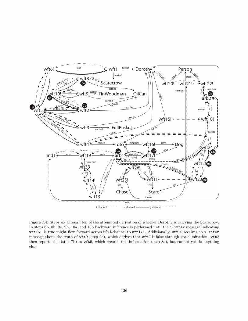
wft1wft6!
wft5
wft8
wft9!wft10!
wft2
wft3
wft4
wft12!
wft11wft25!
wft26!
xor
xor
i�
i�
xor
xor
xor
ant cq
Chase Scare
Toto
FullBasket
OilCan
Dorothy
Scarecrow
TinWoodman
carrier
carrier
carrier
carrier
carried
carried
carried
carrier
carried
act act
theme
experiencer
carried
carried
andorarg [1,2]
andorarg [1,2]andorarg [1,2]
Dog
Person
wft15!
ind1 arb1
wft16!member class
wft17!member
wft18!
wft19 carried
wft20!class
member
wft21!
class
member
arb2
wft22!member
class
carrier
owner
owns
wft23act
wft24
carrier
carried
rest
rict
restrict
restrict
restrict
i-channel u-channel g-channel
experiencer
8a
6a
i-infer
i-infer
cancel-infer
u-infer 7b
7a
6b
8b
9a
9b
10a
10b
owner
owns
class
carrier
wft14!
wft13
xor
xor
selfM
over
wft33close (arb1)
depends
Figure 7.4: Steps six through ten of the attempted derivation of whether Dorothy is carrying the Scarecrow.In steps 6b, 8b, 9a, 9b, 10a, and 10b backward inference is performed until the i-infer message indicatingwft16! is true might flow forward across it’s i-channel to wft17!. Additionally, wft10 receives an i-infermessage about the truth of wft9 (step 6a), which derives that wft2 is false through xor-elimination. wft2then reports this (step 7b) to wft5, which records this information (step 8a), but cannot yet do anythingelse.
126

task queue <wft20! −i→ wft22!>, <wft21! −i→ wft22!>, <wft17! −i→ arb1>,
<wft18! −b→ arb2>, <wft11 −b→ wft23>, <arb1 −b→ wft23>
12a wft22! receives i-infer message from wft20!;
relays the i-infer messages to arb2 since it is an analytic term.
12b wft22! receives i-infer message from wft21!;
relays the i-infer messages to arb2 since it is an analytic term.
task queue <wft22! −i→ arb2> (note: {Dorothy/arb2}), <wft22! −i→ arb2> (note: {ind1/arb2}),
<wft17! −i→ arb1>, <wft18! −b→ arb2>, <wft11 −b→ wft23>, <arb1 −b→ wft23>
13a arb2 receives i-infer message from wft22! with the substitution {Dorothy/arb2};
all restrictions of arb2 are not yet satisfied so nothing more happens here yet.
13b arb2 receives i-infer message from wft22! with the substitution {ind1/arb2};
all restrictions of arb2 are not yet satisfied so nothing more happens here yet.
task queue <wft17! −i→ arb1>, <wft18! −b→ arb2>, <wft11 −b→ wft23>, <arb1 −b→ wft23>
14a arb1 receives i-infer message from wft17!;
This message satisfies the restrictions of arb1, and is relayed to wft23 and wft24.
14b wft18! sends backward-infer messages to wft15! and arb1;
opens the i-channel from wft15! to wft18!, and the g-channel from arb1 to wft18!. Since there is
an i-infer messages waiting in both of these i-channels, they are added to the queue.
task queue <wft15! −i→ wft18!>, <arb1 −i→ wft18!>, <arb1 −i→ wft23>, <arb1 −i→ wft24>,
<wft11 −b→ wft23>, <arb1 −b→ wft23>
15a wft18! receives i-infer message from wft15!;
relays the i-infer messages to arb2 since it is an analytic term.
15b wft18! receives i-infer message from arb1;
relays the i-infer messages to arb2 since it is an analytic term.
task queue <wft18! −i → arb2> (note: {Toto/arb1, Dorothy/arb2}), <wft18! −i → arb2> (note:
{Toto/arb1}),
<arb1 −i→ wft23>, <arb1 −i→ wft24>, <wft11 −b→ wft23>, <arb1 −b→ wft23>
127
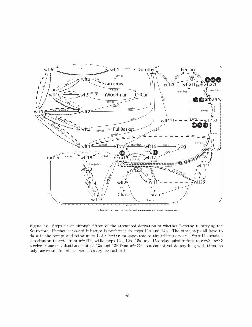
11a
11b12a 12b
13a 13b
14a
14b15a 15b
wft1wft6!
wft5
wft8
wft9!wft10!
wft2
wft3
wft4
wft12!
wft11wft25!
wft26!
xor
xor
i�
i�
xor
xor
xor
ant cq
Chase Scare
Toto
FullBasket
OilCan
Dorothy
Scarecrow
TinWoodman
carrier
carrier
carrier
carrier
carried
carried
carried
carrier
carried
act act
theme
experiencer
carried
carried
andorarg [1,2]
andorarg [1,2]andorarg [1,2]
Dog
Person
wft15!
ind1 arb1
wft16!member class
wft17!member
wft18!
wft19 carried
wft20!class
member
wft21!
class
member
arb2
wft22!member
class
carrier
owner
owns
wft23act
wft24
carrier
carried
rest
rict
restrict
restrict
restrict
i-channel u-channel g-channel
experiencer
owner
owns
class
carrier
i-infer
i-infer
i-infer
i-infer
i-infer
wft14!
wft13
xor
xor
selfM
over
wft33close (arb1)
depends
Figure 7.5: Steps eleven through fifteen of the attempted derivation of whether Dorothy is carrying theScarecrow. Further backward inference is performed in steps 11b and 14b. The other steps all have todo with the receipt and retransmittal of i-infer messages toward the arbitrary nodes. Step 11a sends asubstitution to arb1 from wft17!, while steps 12a, 12b, 15a, and 15b relay substitutions to arb2. arb2receives some substitutions in steps 13a and 13b from wft22! but cannot yet do anything with them, asonly one restriction of the two necessary are satisfied.
128
Figure 7.6 illustrates steps sixteen through nineteen of the inference task attempting to derive that
Dorothy is not carrying the Scarecrow. In these steps backward inference continues from wft23 to wft11
(step 19a) and to arb1 (step 19b). Substitutions from arb1 are collected by wft23 and wft24 in steps 18a and
18b. In steps 16a and 16b, arb2 processes the two substitutions from wft18! ({Toto/arb1, Dorothy/arb2}
and {Toto/arb1}), combines them with previously received substitutions from wft22!, and sends the results
to wft24 (where they’re received in steps 17a and 17b, but nothing else can happen).
16a arb2 receives i-infer message from wft18! with the substitution {Toto/arb1, Dorothy/arb2};
since now both restrictions of arb2 are satisfied in a compatible way (previously, {Dorothy/arb2} was
received from wft22!), arb2 sends an i-infer message to wft24.
16b arb2 receives i-infer message from wft18! with the substitution {Toto/arb1};
when combined with the substitution {ind1/arb2} previously received from wft22!, a new substitution
is created, and an i-infer message is sent to wft24.
task queue <arb2−i→ wft24> (note: {Toto/arb1, Dorothy/arb2}), <arb2−i→ wft24> (note: {Toto/arb1,
ind1/arb2}),
<arb1 −i→ wft23>, <arb1 −i→ wft24>, <wft11 −b→ wft23>, <arb1 −b→ wft23>
17a wft24 receives i-infer message from arb2 with the substitution {Toto/arb1, Dorothy/arb2};
it is not yet satisfied since it does not have a matching instance from arb1 and is not asserted, so it
does nothing else now.
17b wft24 receives i-infer message from arb2 with the substitution {Toto/arb1, ind1/arb2};
it is not yet satisfied since it does not have a matching instance from arb1 and is not asserted, so it
does nothing else now.
task queue <arb1 −i→ wft23>, <arb1 −i→ wft24>, <wft11 −b→ wft23>, <arb1 −b→ wft23>
18a wft23 receives i-infer message from arb1;
since wft23 is unasserted, nothing further an be done.
18b wft24 receives i-infer message from arb1;
in step 17a and 17b, wft24 received {Toto/arb1, Dorothy/arb2} and {Toto/arb1, ind1/arb2}, so it
now has a satisfying set of substitutions from each restriction, but since it is unasserted it does nothing
more.
129
task queue <wft11 −b→ wft23>, <arb1 −b→ wft23>
19a wft11 sends backward-infer message to wft26!;
opens the u-channel from wft26! to wft11.
19b arb1 has no further incoming channels to open.
task queue <wft26! −b→ wft11>
Figure 7.7 shows steps twenty through twenty-four of the derivation of whether or not Dorothy is carrying
the Scarecrow. Step 20 continues backward inference from wft26! to wft25!. Step 21 receives an i-infer
message from wft25! — that Dorothy is being chased — and by the rules if implication derives its consequent
— that Toto is scared. Step 22 relays this new asserted knowledge to wft23, where, combined with the
previously received substitution from arb1, it can now be considered satisfied and a message is sent to
wft12!, where that rule is satisfied and the substitution {Toto/arb1} is sent to wft24. As before, steps
twenty through twenty-four are detailed below.
20 wft26! sends backward-infer message to wft25!;
opens the i-channel from wft25! to wft26!. Since there is a message waiting at the valve in the
channel from wft25! to wft26!, its processing is added to the top of the queue.
task queue <wft25! −i→ wft26!>
21 wft26! receives i-infer message from wft25!;
according to the rules of implication, wft26! is satisfied, and sends a u-infer message to wft11.
task queue <wft26! −u→ wft11>
22 wft11 receives u-infer message from wft26!;
wft11 now asserts itself (it has now been derived that Toto is scared), and sends an i-infer message
to wft23.
task queue <wft11! −i→ wft23>
23 wft23 receives i-infer message from wft11;
given this, and the substitution already received from arb1 that {Toto/arb1}, wft23 is instantiated,
and sends an i-infer message to wft12!.
task queue <wft23 −i→ wft12!>
130

i-channel u-channel g-channel
16b16a
17b
17a
18a
18b
19b
19a
wft1wft6!
wft5
wft8
wft9!wft10!
wft2
wft3
wft4
wft12!
wft11wft25!
wft26!
xor
xor
i�
i�
xor
xor
xor
ant cq
Chase Scare
Toto
FullBasket
OilCan
Dorothy
Scarecrow
TinWoodman
carrier
carrier
carrier
carrier
carried
carried
carried
carrier
carried
act act
theme
experiencer
carried
carried
andorarg [1,2]
andorarg [1,2]andorarg [1,2]
Dog
Person
wft15!
ind1 arb1
wft16!member class
wft17!member
wft18!
wft19 carried
wft20!class
member
wft21!
class
member
arb2
wft22!member
class
carrier
owner
owns
wft23act
wft24
carrier
carried
rest
rict
restrict
restrict
experiencer
owner
owns
class
carrier
i-infer
i-infer
i-infer
i-infer
wft14!
wft13
xor
xor
selfM
over
wft33close (arb1)
depends
Figure 7.6: Steps sixteen through nineteen of the attempted derivation of whether Dorothy is carryingthe Scarecrow. Backward inference continues from wft23 to wft11 (step 19a) and to arb1 (step 19b).Substitutions from arb1 are collected by wft23 and wft24 in steps 18a and 18b. In steps 16a and 16b, arb2processes the two substitutions from wft18! ({Toto/arb1, Dorothy/arb2} and {Toto/arb1}), combines themwith previously received substitutions from wft22!, and sends the results to wft24 (where they’re receivedin steps 17a and 17b, but nothing else can happen).
131

24 wft12! receives i-infer message from wft23;
according to the rules of iff, wft12! is satisfied, and sends a u-infer message to wft24.
task queue <wft12! −i→ wft24>
Figure 7.8 shows steps twenty-five through thirty-one of the derivation of whether or not Dorothy is
carrying the Scarecrow. Since Toto is scared, and the rule wft12! that if a dog is scared, then its owner
carries it, it is derived in step 25 that Toto’s owner carries Toto. This new assertion is shown in Figure 7.8
as wft30!. Associated with this are several new terms, detailed below.
wft30!: (Carries (every x Person (owns Toto)) Toto)
wft31!: (Owns (every x Person (owns Toto)) Toto)
wft32!: (Isa (every x Person (owns Toto)) Person)
arb3: (every x Person (owns Toto))
After wft30! is derived, wft24 sends an i-infer message to wft4. Because wft4 is part of a backward
inference task, and wft30! can derive wft4, backward inference occurs from wft4 backward to wft30!. As
such, an i-infer message (identical to that from wft24 flows to wft4. Since these two identical messages
do not mention Dorothy, they are discarded when it is attempted to pass them onward to wft4. The rest of
the steps deal with continuing backward inference from wft30, into arb3 and its restrictions, and gathering
instances at those restrictions (similarly to what happened with arb2 in steps 11-16).
25 wft24 receives u-infer message from wft12!;
from this it is derived that wft30!, Toto is carried by Toto’s owner. This result is sent to wft4 through
the i-channel from wft24 to wft4, but it does not pass the filter in that channel, so is discarded. Since
wft30! has now been created, has a channel to wft4, and wft4 is part of a backward inference task,
focused inference continues backward inference to wft30!. wft30! has an instance which it sends to
wft4 (the same one wft24 has, so it is also discarded).
task queue <wft4 −b→ wft30!>
26 wft30! sends backward-infer message to arb3;
opens the g-channel from arb3 to wft30!.
task queue <arb3 −b→ wft30!>
132

i-channel u-channel g-channel
20
2122
23
24
wft1wft6!
wft5
wft8
wft9!wft10!
wft2
wft3
wft4
wft12!
wft11wft25!
wft26!
xor
xor
i�
i�
xor
xor
xor
ant cq
Chase Scare
Toto
FullBasket
OilCan
Dorothy
Scarecrow
TinWoodman
carrier
carrier
carrier
carrier
carried
carried
carried
carrier
carried
act act
theme
experiencer
carried
carried
andorarg [1,2]
andorarg [1,2]andorarg [1,2]
Dog
Person
wft15!
ind1 arb1
wft16!member class
wft17!member
wft18!
wft19 carried
wft20!class
member
wft21!
class
member
arb2
wft22!member
class
carrier
owner
owns
wft23act
wft24
carrier
carried
rest
rict
restrict
restrict
experiencer
owner
owns
class
carrier
i-inf
er
u-infer i-inferwft14!
wft13
xor
xor
selfM
over
wft33close (arb1)
depends
Figure 7.7: Steps twenty through twenty-four of the derivation of whether or not Dorothy is carrying theScarecrow. Step 20 continues backward inference from wft26! to wft25!. Step 21 receives an i-infermessage from wft25! — that Dorothy is being chased — and by the rules if implication derives its consequent— that Toto is scared. Step 22 relays this new asserted knowledge to wft23, where, combined with thepreviously received substitution from arb1, it can now be considered satisfied and a message is sent towft12!, where that rule is satisfied and the substitution {Toto/arb1} is sent to wft24.
133

27 arb3 sends backward-infer messages to wft31! and wft32!;
opens the g-channels from wft31! and wft32! to arb3.
task queue <wft31! −b→ arb3>, <wft32! −b→ arb3>
28a wft31! sends backward-infer message to wft15!;
opens the i-channel from wft15! to wft31!. There is an i-infer message waiting, which flows forward
to wft31!.
28b wft32! sends backward-infer messages to wft20! and wft21!;
opens the i-channels from wft20! and wft21! to wft32!. There are i-infer messages waiting in both
channels, which flows forward to wft31!.
task queue <wft20! −i→ wft32!>, <wft21! −i→ wft32!>, <wft15! −i→ wft31!>
29a wft32! receives i-infer message from wft20!;
Since wft32! is an analytic generic term, it relays the received substitution: {Dorothy/arb3} to arb3.
29b wft32! receives i-infer message from wft21!;
Since wft32! is an analytic generic term, it relays the received substitution: {ind1/arb3} to arb3.
task queue <wft32! −i→ arb3> (note: {Dorothy/arb3}), <wft32! −i→ arb3> (note: {ind1/arb3}),
<wft15! −i→ wft31!>
30a arb3 receives i-infer message from wft32! with substitution {Dorothy/arb3};
since this message only satisfies one restriction, the message is saved until later.
30b arb3 receives i-infer message from wft32! with substitution {ind1/arb3};
since this message only satisfies one restriction, the message is saved until later.
task queue <wft15! −i→ wft31!>
31 wft31! receives i-infer message from wft15!;
Since wft31! is an analytic generic term, it relays the message to arb3.
task queue <wft31! −i→ arb3>
Figure 7.9 shows the conclusion, steps thirty-two through thirty-seven, of the derivation of whether or
not Dorothy is carrying the Scarecrow. In step 32, arb3 receives substitutions from wft31 and determines
134

i-channel u-channel g-channel
3128a
25 26wft30!
arb3
wft32!
class
memberrest
rict
owner
carrier
restrict
28b
29a
29b
30a
30b
27
i-infer
wft1wft6!
wft5
wft8
wft9!wft10!
wft2
wft3
wft4
wft12!
wft11wft25!
wft26!
xor
xor
i�
i�
xor
xor
xor
ant cq
Chase Scare
Toto
FullBasket
OilCan
Dorothy
Scarecrow
TinWoodman
carrier
carrier
carrier
carrier
carried
carried
carried
carrier
carried
act act
theme
experiencercarried
carried
andorarg [1,2]
andorarg [1,2]andorarg [1,2]
Dog
Person
wft15!
ind1 arb1
wft16!member class
wft17!member
wft18!
wft19 carried
wft20!class
member
wft21!
class
member
arb2
wft22!member
class
carrier
owner
owns
wft23act
wft24
carrier
carried
rest
rict
restrict
restrict
experiencer
owner
owns
class
carrier
wft31!owns
i-infer
i-inferi-infer
i-infer
i-infer
wft14!
wft13
xor
xor
selfM
over
wft33close (arb1)
depends
Figure 7.8: Steps twenty-five through thirty-one of the derivation of whether or not Dorothy is carrying theScarecrow. These steps have largely to do with satisfying the new arbitrary term arb3, added when therule wft12! fired, creating wft30!. Backward inference occurred from wft4 to wft30! because of focusedreasoning. See the text for a detailed description of these steps.
135

that it is satisfied, sending messages onward to wft30!, then to wft4 (step 33), and to wft5 (step 34). Since
it’s now derived that Dorothy carries Toto, the andor represented by wft5 may be introduced (step 35), and
the xor at wft6! may fire (step 436, deriving that Dorothy does not carry the Scarecrow (step 37).
32 arb3 receives i-infer message from wft31!;
this message indicates that Dorothy is the owner of Toto, and the other restriction already learned
that Dorothy is a person, so arb3 is satisfied and sends a message to wft30!.
task queue <arb3 −i→ wft30!>
33 wft30! receives i-infer message from arb3;
this message is from the only arbitrary contained within wft30! so wft30! is fully satisfied, and since
it’s believed, it is derived that Dorothy carries Toto. This result is sent to wft4.
task queue <wft30! −i→ wft4>
34 wft4 receives i-infer message from wft30!;
wft4 — that Toto is carried by Dorothy — can now be believed, and a message is sent to wft5.
task queue <wft4! −i→ wft5>
35 wft5 receives i-infer message from wft4!;
given the rule for andor introduction, wft5 can now be derived. An i-infer message is sent from
wft5! to wft6.
task queue <wft5 −i→ wft6>
36 wft6! receives i-infer message from wft5!;
given the rule for xor elimination, the negation of wft1 can now be derived, and as such a u-infer
message is sent from wft6! to wft1.
task queue <wft6! −u→ wft1>
37 wft1 receives u-infer message from wft6!;
the negation of wft1, that Dorothy does not carry the Scarecrow is derived.
136

i-channel u-channel g-channel
37
32
36
35
34
33wft30!
arb3
wft32!
class
memberrest
rict
owner
carrier
restrict
wft1wft6!
wft5
wft8
wft9!wft10!
wft2
wft3
wft4
wft12!
wft11wft25!
wft26!
xor
xor
i�
i�
xor
xor
xor
ant cq
Chase Scare
Toto
FullBasket
OilCan
Dorothy
Scarecrow
TinWoodman
carrier
carrier
carrier
carrier
carried
carried
carried
carrier
carried
act act
theme
experiencer
carried
carried
andorarg [1,2]
andorarg [1,2]andorarg [1,2]
Dog
Person
wft15!
ind1 arb1
wft16!member class
wft17!member
wft18!
wft19 carried
wft20!class
member
wft21!
class
member
arb2
wft22!member
class
carrier
owner
owns
wft23act
wft24
carrier
carried
rest
rict
restrict
restrict
experiencer
owner
owns
class
carrier
wft31!owns
i-infer
i-infer
i-infer
i-infer
i-inf
er
u-infer
wft14!
wft13
xor
xor
selfM
over
wft33close (arb1)
depends
Figure 7.9: Steps thirty-two through thirty-seven, of the derivation of whether or not Dorothy is carryingthe Scarecrow. These steps show the propagation of messages from arb3 eventually to wft1 deriving thatDorothy is not carrying the Scarecrow. See the text for a more detailed description.
137
7.3 Inference Procedures
Every time inference is invoked by the user, we say a new inference procedure has begun. It sometimes is
necessary to recognize when a particular inference procedure has reached a quiescent state, independent of
the entire graph’s state. This is particularly apparent in the acting system, where an action may need to
execute further inference procedures, and determine when they have completed (to the extent possible).
In order to accomplish this, each inference process is associated with a counter. The counter is incre-
mented every time a message related to that process is added to the processing queue, and decremented
once the message has been fully consumed and processed (that is, after any resulting messages have al-
ready been added to the queue). The counter begins at zero, and when it once again arrives at zero, the
inference procedure is complete.3 In this way the progress of multiple inference procedures can be tracked
independently.
7.4 Evaluation of Concurrency4
The massively parallel logical inference systems of the 1980s and 90s often assigned each processor a single
formula or rule to be concerned with. This resulted in limits on the size of the KB (bounded by the number of
processors), and many processors sitting idle during any given inference process. Our technique dynamically
assigns tasks to threads only when they have work to do, meaning that processors are not sitting idle so long
as there are as many tasks available as there are processors.
In evaluating the performance of the concurrency mechanisms at play in the IG, we are mostly concerned
with the speedup achieved as more processors are used in inference. Overall processing time is also important,
but will be primarily of concern in the next chapter. More relevant to our current discussion is the issue of
speedup. If speedup is roughly linear with the number of processors, then that will show that the architecture
and heuristics discussed in this dissertation scale well. We will look at the performance of our system in both
backward and forward inference. The other two types of inference — bi-directional inference, and focused
reasoning — are hybrids of forward and backward inference, and have performance characteristics between
the two.3This is guaranteed to happen at the appropriate time: the counter is only decremented after a message is fully processed
(meaning that any resulting messages have been added to the processing queue, and therefore incremented the counter), andevery message which is added to the queue is eventually processed.
4This section uses a similar evaluation methodology as that of (Schlegel and Shapiro, 2014a), and while it is adapted fromthat paper, includes wholly new results as IGs have evolved a great deal since that was published.
138

7.4.1 Backward Inference
To evaluate the performance of the inference graph in backward inference, we generated graphs of chaining
entailments. Each entailment had bf antecedents, where bf is the branching factor, and a single consequent.
Each antecedent and consequent made use of the same single arbitrary term containing a single restriction.5
Each consequent was the consequent of exactly one rule, and each antecedent was the consequent of another
rule, up to a depth of d entailment rules. Exactly one consequent, cq, was not the antecedent of another
rule. Therefore there were bf d entailment rules, and 2 ∗ bf d − 1 antecedents/consequents. A single instance
of each of the bf d leaf nodes was asserted, along with an appropriate satisfier of the shared arbitrary term’s
restriction. We tested the ability of the system to backchain on and derive a specific instance of cq when
the entailments used were both and-entailment and or-entailment. Backward inference is the most resource
intensive type of inference the inference graphs can perform, and most fully utilizes the scheduling heuristics
in this chapter.
In the first test we used and-entailment, meaning for each implication to derive its consequent, all its
antecedents had to be true. Since we backchained on an instance of cq, this meant instances of every rule
consequent and antecedent in the graph would have to be derived. This is the worst case scenario for
entailment. The timings we observed are presented in Table 7.1.6 This experiment showed that speedup
grows linearly7 as more CPUs are involved in inference.8
Table 7.1: Inference times using 1, 2, 4, and 8 CPUs for 100 iterations of and-entailment in an inferencegraph with bf = 2 and d = 7.
CPUs Inference Time (ms) Speedup1 229631 1.002 122986 1.874 65979 3.488 35982 6.38
The next experiments tested whether the depth or branching factor of the graph has any effect on
speedup as the number of processors increases. The first experiment judged the impact of graph depth.5Adjusting the number of arbitrary terms or restrictions used has a very small impact in this example, as calculation of
instances is performed only once per arbitrary, and the arbitrary or arbitraries need to be shared by all nodes to performmeaningful inference. It is in line with normal use of LA to have relatively few arbitrary terms.
6All tests were performed on a Dell Poweredge 1950 server with dual quad-core Intel Xeon X5365 processors (no Hyper-Threading) and 32GB RAM. Each test was performed twice, with the second result being the one used here. The first run wasonly to allow the JVM to “warm up.” This machine is shared-use, and as such, some minor irregularities in the results shouldbe expected.
7y = 0.7639x + 0.3178, R2 = 0.99878In previous experiments (Schlegel and Shapiro, 2014a) using ground propositional logic, it was necessary to subtract a
constant from each result to see linear speedup, due to a centralized method of storing what terms were asserted, and theassociated difficulty of maintaining shared state. The use of origin sets decentralizes this, and therefore this adjustment is nolonger necessary.
139

The experiment was run on graphs of five different depths, ranging from 5 to 10 (32 leaves, to 1024 leaves),
while maintaining bf = 2 (see Figure 7.109), and found that as graph depth is increased, speedup is nearly
constant.
0
1
2
3
4
5
6
7
5 6 7 8 9 10
Speedu
p
Depth of Graph
Speedup vs. Depth of Graph
1 CPU
2 CPUs
4 CPUs
8 CPUs
Figure 7.10: Speedup of the and-entailment test, shown in relation to the depth of the inference graph. Asthe depth of the graph increases speedup remains nearly constant. A branching factor of 2 was used in alltests.
To find out if branching factor affects speedup, d = 5 was chosen, and the branching factor was varied
from 1 to 6 (1 to 7,776 leaves). When bf = 1, the graph is simply a chain of nodes, and the use of more
processors can provide very little improvement in computation time. As shown in Figure 7.11, throwing more
processors at the problem eventually just causes no improvement. Fortunately, this is a rather contrived use
of the inference graph. At branching factors 2-6, the graph performs as expected, with the branching factor
increase having little effect on performance. There may be a slight performance impact as the branching
factor increases, because at higher branching factors more messages must be combined at each rule node.
The data does not show this definitively though.
In our second test we used the same KB from the first (d = 7, bf = 2), except each and-entailment rule
was swapped for or-entailment. Whereas the earlier test required an instance of every generic term in the
KB to be derived, this test shows the best case of entailment — an instance of only a single leaf must be
derived to allow the chaining causing the selected instance of cq to be derived.9Exact values used in Figure 7.10 and Figure 7.11 are presented in Appendix A.
140

0
1
2
3
4
5
6
7
1 2 3 4 5 6
Speed
up
Branching Factor
Speedup vs. Branching Factor
1 CPU
2 CPUs
4 CPUs
8 CPUs
Figure 7.11: Speedup of the and-entailment test, shown in relation to the branching factor of the inferencegraph. A depth of 5 was used in all tests, to keep the number of nodes reasonable.
Table 7.2: Inference times, and number of rule nodes used, using 1, 2, 4, and 8 CPUs for 100 iterations ofor-entailment in an inference graph (d = 7, bf = 2) in which there are many paths through the network (allof length 7) that could be used to infer the result.
CPUs Time (ms) Average Number of Rules Fired Speedup Speedup vs. and-entailment1 104099 7 1.00 2.212 57949 11 1.80 2.124 32364 18 3.22 2.048 28429 33 3.66 1.27
The improvement in or-entailment processing times as we add more CPUs (see Table 7.2) is not as
dramatic since the inference operation performed once a chain of valve selectors from a derived instance of a
leaf to the instance of cq are added cannot be accelerated by adding more processing cores — that process
is inherently sequential. The improvement we see increasing from 1 to 2, and 2 to 4 CPUs is because the
backward-infer and cancel-infer messages spread throughout the network breadth-first and can be sped
up through concurrency. During the periods where backward inference has already begun, and cancel-infer
messages are not being sent, the extra CPUs were working on deriving formulas relevant to the current query,
but in the end unnecessary — as seen in the number of rule nodes fired in Table 7.2. The time required for
these derivations begins to outpace the improvement gained through concurrency when we reach 8 CPUs in
this task. These extra derivations may be used in future inference tasks, though, without re-derivation, so
the resources are not wasted. As only a chain of rules is required, altering branching factor or depth has
141

no effect on speedup. It is interesting to note that for the cases where 1-4 CPUs are used, or-entailment is
roughly twice as fast as and-entailment.
The difference in computation times between the or-entailment and and-entailment experiments are
largely due to the scheduling heuristics described in Sect. 7.2. Without the scheduling heuristics, backward
inference tasks continue to get executed even once messages start flowing forward from the leaves. Addi-
tionally, more rule nodes fire than are necessary, even in the single processor case. We ran the or-entailment
test again without these heuristics using a FIFO queue, and found the inference took much longer than
in Table 7.1 (sometimes by over 40x, see Table 7.3), and showed very poor characteristics as the number
of processors was increased due to the terribly inefficient ordering of messages. We then tested a LIFO
queue since it has some of the characteristics of our prioritization scheme (see Table 7.4), and found our
prioritization scheme to be between 4 and 7x faster. It can therefore be stated with some certainty that the
scheduling heuristics we’ve presented are significantly better than naive approaches.
Table 7.3: The same experiment as Table 7.2 replacing the improvements discussed in Sect. 7.2, with a FIFOqueue. Our results in Table 7.2 are between 7 and 40 times faster.
CPUs Time (ms) Averave Number of Rules Fired Speedup Speedup vs. Prioritized Queue1 829920 127 1.00 0.132 693721 127 1.20 0.084 860425 127 0.96 0.048 1179236 127 0.70 0.02
Table 7.4: The same experiment as Table 7.2 replacing the improvements discussed in Sect. 7.2, with a LIFOqueue. Our results in Table 7.2 are between 4 and 7 times faster.
CPUs Time (ms) Average Number of Rules Fired Speedup Speedup vs. Prioritized Queue1 459490 11 1.00 0.232 405009 25 1.13 0.144 145883 47 3.15 0.228 84584 86 5.43 0.19
7.4.2 Forward Inference
To evaluate the performance of the inference graph in forward inference, we again generated graphs of
chaining entailments. Each entailment had a single antecedent, and 2 consequents. Each consequent was the
consequent of exactly one rule, and each antecedent was the consequent of another rule, up to a depth of 7
entailment rules. Exactly one antecedent, ant, the “root”, was not the consequent of another rule. There
were 128 consequents that were not antecedents of other rules, the leaves. Each antecedent and consequent
142

again shared a single arbitrary term with a single restriction. We tested the ability of the system to derive
instances of the leaves when the instance of ant, and the instance of the arbitrary term’s restriction were
asserted with forward inference.
Since all inference in our graphs is essentially forward inference (modulo additional message passing to
manage the valves), and we’re deriving the same number of terms, one might expect the results from our
forward inference test to be similar to those of backward inference using and-entailment rules. This is not the
case. In this example, many more origin sets are calculated. This makes sense, since in backward inference,
multiple messages with different origin sets may be generated at a rule node, and sent to its consequents. Not
all of these necessarily pass the valve selectors (where in forward inference they would all be passed onward),
and once one satisfying message passes a valve selector and is consumed, its priority is increased, meaning
the other ones which were created may never be consumed before the task is canceled. In the backward
inference using and-entailment example, an average of 401 origin sets were derived, with an average size of
1.87. In this example, an average of 1092 origin sets are calculated, with an average size of 4.33. That means
this example required approximately 6.3 times the work in calculating origin sets.
The results of this test are shown in Table 7.5. Once again we find that speedup is linear with the number
of processors.10 We can therefore say with confidence that IGs exhibit a speedup linear in time with the
number of processors for forward inference.
Table 7.5: Inference times using 1, 2, 4, and 8 CPUs for 100 iterations of forward inference in an inferencegraph of depth 7 and branching factor 2 in which all leaf nodes are derived.
CPUs Inference Time (ms) Speedup1 1483882 1.002 854528 1.744 482435 3.088 238550 6.22
10y = 0.7447x + 0.2174, R2 = 0.9989
143

Chapter 8
Using Inference Graphs as Part of a
Natural Language Understanding
System
In order to evaluate the performance of IGs on a real world task, they have been employed as the reasoner
in a natural language understanding task. In this task, IGs are used to find appropriate instances of, and
execute syntax-semantics mapping rules. The implemented mapping rules are adopted from the Tractor
natural language understanding system (Prentice et al., 2010; Gross et al., 2012; Shapiro and Schlegel,
2013). As a whole, the mapping rules convert a syntactic knowledge base, derived from various natural
language processing processes applied to short intelligence messages from the counter-insurgence domain, to
one containing mostly semantic information.
This chapter first introduces the Tractor natural language understanding system in Section 8.1, including
a discussion of the role of the mapping rules. A rule engine has been developed as part of CSNePS for pattern
matching tasks, including the mapping rules, discussed in Section 8.2. Some illustrative mapping rules are
presented in the language of the CSNePS rule engine in Section 8.3, and evaluation of the implemented rules
as compared to the Tractor implementation in SNePS 3, and an implementation in SNePS 2 is presented in
Section 8.4.
144
8.1 Tractor1
Tractor performs natural language understanding, translating text into a semantic propositional graph, by
sending text through a pipeline of four different components, each consisting of several subcomponents. First,
standard natural language processing techniques are performed upon the text using the General Architecture
for Text Engineering (GATE) (The University of Sheffield, 2011). GATE produces sets of annotations for
spans of text, which are combined, and translated into a propositional graph in the Propositionalizer. Our
Context-Based Information Retrieval (CBIR) system enhances the propositional graph with ontological and
geographical information. Finally the enhanced mostly syntactic graphs are translated into semantic propo-
sitional graphs by the syntax-semantics mapping rules. Of principal interest here is the syntax-semantics
mapping rules.
The purpose of the syntax-semantics mapping rules is to convert information expressed as sets of syntactic
assertions into information expressed as sets of semantic assertions. The rules were hand-crafted by examining
syntactic constructions in subsets of our corpus, and then expressing the rules in general enough terms so
that each one should apply to other examples as well.
We have already performed evaluation (Shapiro and Schlegel, 2013) of the mapping rules and found them
to be sufficiently general (but not overly so), and provided good coverage of the syntactic data found in both
our evaluation and test datasets, resulting in over 90% semantic knowledge in the resulting KB.
The full set of mapping rules are implemented using the SNePS 3 rule engine, designed specifically for
this task. A subset of the rules have been implemented in SNePS 2 and the CSNePS Rule Language, which
is defined and discussed in the following section.
8.2 CSNePS Rule Language
CSNePS implements a rule language loosely based on a subset of the syntax of CLIPS (Riley and Dantes,
2007), and using concepts from the GLAIR Cognitive Architecture (Shapiro and Bona, 2010). A rule
definition takes the following general form:
rule = ‘(defrule’, rulename, LHS, ‘=>’ RHS ‘)’;
where rulename is a unique name for a rule, LHS is the Left Hand Side of the rule (the “pattern matching”
component2), and RHS is the Right Hand Side of the rule (the firing component). The LHS and RHS are1Portions of this section are adapted and updated from (Shapiro and Schlegel, 2013).2Really, inference is performed to derive instances of patterns.
145

discussed in more detail in Sections 8.2.1 and 8.2.2. The implementation of rules as part of an acting system
is discussed in Section 8.2.3.
8.2.1 The Left Hand Side
The LHS of a rule is a collection of generic terms that must be matched for the rule to fire. This portion
of the rule is special in that the quantified terms used take wide scope over the entire rule. Continuing the
formal definition of the rule language, the LHS is defined as follows:
LHS = genericterm+;
where genericterm is the definition of generic terms that we’ve used throughout this dissertation.
8.2.2 The Right Hand Side
The RHS of a rule may contain both Clojure forms and subrules. The set of Clojure forms will be executed
in order, and the bindings from the LHS will be substituted in to them. Subrules are rules that are unnamed,
and are only executed when the RHS of a rule fires. The subrule is provided the set of LHS bindings, which
it may use in its own LHS/RHS. Subrules may themselves have subrules, with no constraint on depth.
Again continuing the formal definition of the rule language, the RHS is defined as follows:RHS = RHSLine+;
RHSLine = clojureform | subrule;
subrule = ‘(:subrule’ LHS ‘=>’ RHS ‘)’;
8.2.3 Rules as Policies
A policy in an acting system allows Propositions to be connected in some way with actions. Actions are often
primitive, implemented as Clojure code, but using the bindings from the matched propositions. CSNePS
rules are implemented as policies, where the LHS contains the propositions to be matched, and the RHS
contains the action that should occur.
The rule policy is defined as follows, using CSNePS slots and caseframes. The rule as given in the
language is translated into this form by the build system.
(defineSlot action :type Action
:docstring "The actions of an act."
:min 1 :max 1
:posadjust none :negadjust none)
146

(defineSlot condition :type Propositional
:docstring "conditions for a rule."
:min 1 :posadjust expand :negadjust reduce)
(defineSlot rulename :type Thing
:docstring "The name of a rule."
:min 1 :max 1 :posadjust none :negadjust none)
(defineSlot subrule :type Policy
:docstring "subrules of a rule."
:min 0 :posadjust expand :negadjust reduce)
(defineCaseframe 'Policy '('rule rulename condition action subrule)
:docstring "for the rule [name] to fire, [condition] must be matched,
then [action] may occur, and [subrule] may be matched."))
Policies may not be believed or disbelieved like Propositions. Instead, they may be adopted or unadopted.
A policy that is adopted is active, and one that is unadopted is not. When a rule policy is adopted, backward
inference is performed on each of the LHS propositions, and each subrule is adopted. There is only a single
representation for each subrule built in the IG; subrules are not instantiated when parent rules are matched.
Also, subrules necessarily rely on at least one of its parent rule’s bindings, and may only receive those
bindings from that parent rule. It is for this reason that the subrules of a rule may be adopted when the rule
is.3 When a rule policy is unadopted, the backward inference is canceled, and each subrule is unadopted.
8.3 Example Mapping Rules
In order to illustrate the operation of the mapping rules, consider the following two rules.
(defrule subjAction
(nsubj (every action Token AgentAction) (every subj Token))
=>
(assert `(~'agent ~action ~subj))
(unassert `(~'nsubj ~action ~subj)))3In some cases it is likely more optimal to only adopt subrules when the LHS of a rule is satisfied at least once. This has
not yet been explored.
147
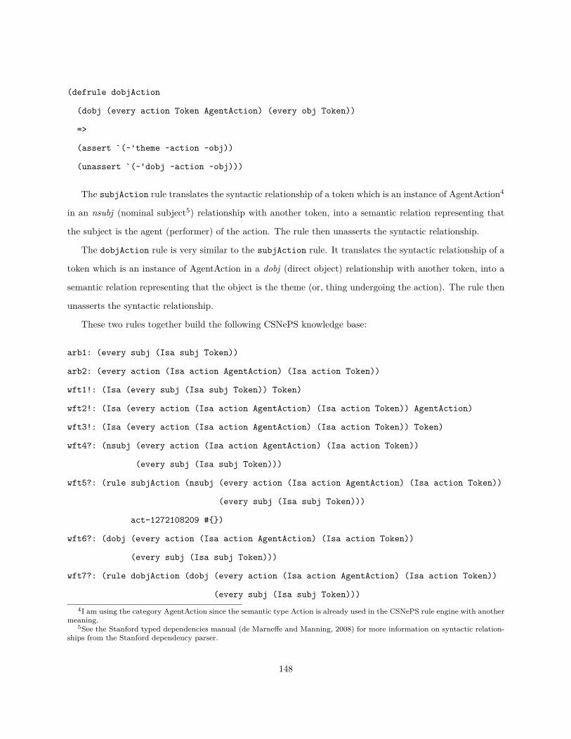
(defrule dobjAction
(dobj (every action Token AgentAction) (every obj Token))
=>
(assert `(~'theme ~action ~obj))
(unassert `(~'dobj ~action ~obj)))
The subjAction rule translates the syntactic relationship of a token which is an instance of AgentAction4
in an nsubj (nominal subject5) relationship with another token, into a semantic relation representing that
the subject is the agent (performer) of the action. The rule then unasserts the syntactic relationship.
The dobjAction rule is very similar to the subjAction rule. It translates the syntactic relationship of a
token which is an instance of AgentAction in a dobj (direct object) relationship with another token, into a
semantic relation representing that the object is the theme (or, thing undergoing the action). The rule then
unasserts the syntactic relationship.
These two rules together build the following CSNePS knowledge base:
arb1: (every subj (Isa subj Token))
arb2: (every action (Isa action AgentAction) (Isa action Token))
wft1!: (Isa (every subj (Isa subj Token)) Token)
wft2!: (Isa (every action (Isa action AgentAction) (Isa action Token)) AgentAction)
wft3!: (Isa (every action (Isa action AgentAction) (Isa action Token)) Token)
wft4?: (nsubj (every action (Isa action AgentAction) (Isa action Token))
(every subj (Isa subj Token)))
wft5?: (rule subjAction (nsubj (every action (Isa action AgentAction) (Isa action Token))
(every subj (Isa subj Token)))
act-1272108209 #{})
wft6?: (dobj (every action (Isa action AgentAction) (Isa action Token))
(every subj (Isa subj Token)))
wft7?: (rule dobjAction (dobj (every action (Isa action AgentAction) (Isa action Token))
(every subj (Isa subj Token)))4I am using the category AgentAction since the semantic type Action is already used in the CSNePS rule engine with another
meaning.5See the Stanford typed dependencies manual (de Marneffe and Manning, 2008) for more information on syntactic relation-
ships from the Stanford dependency parser.
148

act1263530313 #{})
You’ll notice that both rules are able to make use of the same two arbitrary terms. The two generic terms
which combine the substitutions from the arbitrary terms simply send different sets of combinations to the
appropriate rule. Gathering substitutions in shared arbitrary terms allows for less repetition of inference.
To see these rules in action, consider the following knowledge base which is a subset of a knowledge base
for an actual message used in testing:
(TextOf passed n19)
(TextOf Intelligence n17)
(TextOf names n23)
(Isa n17 Token)
(Isa n19 Token)
(Isa n23 Token)
(Isa n19 AgentAction)
(nsubj n19 n17)
(dobj n19 n23)
This comes from a segment of a message whose text is “Iraqi Domestic Counter-Intelligence passed the
names of six prominent Sunni criminal leaders operating in Rashid to Coalition Forces.” Tokens have numeric
identifiers prefixed with the letter “n”, derived from their GATE annotation IDs. The above knowledge base
represents a small portion of the dependency parse of this message, the nsubj relation between the tokens
with text “Intelligence” and “passed”, and the dobj relation between the tokens for the text “passed” and
“names”. After the rules are run, the knowledge base contains the following asserted propositions:
(TextOf passed n19)
(TextOf Intelligence n17)
(TextOf names n23)
(Isa n17 Token)
(Isa n19 Token)
(Isa n23 Token)
(Isa n19 AgentAction) (or perhaps, any individuals at all).
(agent n19 n17)
(theme n19 n23)
149
The resulting knowledge base says that the agent of the “pass” action is “Intelligence” (the root of Iraqi
Domestic Counter-Intelligence), and the theme of the “pass” action is “names”.
8.4 Evaluation of Mapping Rule Performance
In order to evaluate the performance of the IG in performing inference using the mapping rules in a real
world task, 12 rules which were previously implemented using the SNePS 3 rule engine were implemented
in both CSNePS and SNePS 2. The twelve mapping rules selected are some of those which fire the most
number of times on a 114 message subset of SYNCOIN known as the Sunni Criminal Thread (or SUN for
short). Each message is short (one to three sentences), and represents some intelligence information. The
complete set of inference rules implemented in the three systems for this evaluation are given in Appendix B.
The SNePS 3 rule engine was built specifically for the execution of the mapping rules. In that system, the
rules are implemented in Lisp, and compiled to machine code. Most of the time, this system does not really
perform any inference. Rather, it uses a pattern matching strategy against the knowledge base. Occasionally,
where necessary, path-based inference is used, but there is no deductive inference. This strategy does not
extend to inference problems containing variables, but is sufficient for the mapping rules. Rules are executed
one at a time, in a pre-defined order.
The SNePS 2 implementation of the mapping rules uses deductive reasoning and the SNePS Rational
Engine (SNeRE) to believe and disbelieve propositions. This approach requires that all propositions in the
knowledge base be asserted with forward inference. Rules are not tried in any particular order, the ACG
simply matches each new term with antecedents of deductive rules, or conditions of SNeRE acting rules, and
uses the ACG to perform inference.
The CSNePS implementation of the mapping rules uses the scheme described earlier in this chapter. Sets
of rules are adopted in a pre-defined order. A set to be adopted may contain just a single rule, or many.
When the IG reaches a quiescent state after adopting a set of rules, the next set is adopted. The actual
order of rule firing within these sets is determined only by the priorities assigned to messages as in other
types of inference.
To perform the evaluation, the 12 mapping rules were run on each of the 114 messages using each of
the systems. The CSNePS run made use of 8 CPUs, the maximum the hardware available to me supports.
Neither of the other two systems are capable of taking advantage of multiple processors, so they used only
a single CPU.
150

Table 8.1: Time to complete the execution of the 12 selected mapping rules on the 114 message SUN dataset,along with the time for a single message.
Inference Tool Inference Time for 114 Messages (ms) Inference Time for 1 Message (ms)CSNePS IG 831721 7296
SNePS 2 ACG* 144000000 N/ASNePS 3 Rule Engine 53900 473
The performance results are presented in Table 8.1. From these results we see that the SNePS 3 rule
engine is the fastest, taking around half a second per message. CSNePS and the IG came in second, taking
just over seven seconds per message. SNePS 2 and it’s ACG came in a distant third, having been halted
after spending 40 hours processing. The times reported exclude the time taken to load the knowledge base
for each message.
At first glance, it may appear that SNePS 3’s rule engine being an order of magnitude faster is bad news
for IGs, but I claim this is not so. The implementation of these rules in SNePS 3 has taken years of work,
allowing inefficiencies in SNePS 3 itself to be worked out, the rules to be optimized, and the rule engine to be
designed and implemented specifically for this task. This is as opposed to the implementation in CSNePS,
in which the rules were implemented over a short time period with no major optimization to the system or
the rules. In addition, the inference system used by CSNePS is general, and not geared specifically for this
task. It is also the case that the gap narrows as more CPUs are added to the CSNePS version, as we’ve seen
in the previous chapter.
On a real use-case we have shown that, for a performance penalty that diminishes with compute power,
you could use CSNePS to get the system up and running with decent performance (much better than
SNePS 2, which is its most similar competitor in capabilities) without spending a ton of time optimizing, or
developing a task-specific tool.
Table 8.2: Time to process the subjAction rule in CSNePS (using the IG), SNePS 2 (using the ACG),and the SNePS 3 rule engine on the 114 message SUN dataset, as compared to the time to process boththe subjAction and dobjAction rules using those same systems on the same dataset. The times presentedexclude the time needed to load the knowledge base into each system. The difference in time (∆Time) andpercent increase between these two tests shows the advantage of sharing components of the LHS of rules.
Rule Processor subjAction (ms) subjAction + dobjAction (ms) ∆Time % IncreaseCSNePS IG 78558 81413 2855 3.63%
SNePS 2 ACG 5378698 8052874 2674176 49.72%SNePS 3 Rule Engine 4400 9000 4600 104.55%
One of the major advantages of the graph-based approach used in CSNePS is the ability to share parts
of the LHS of rules. The use of shared portions of LHS conditions can be seen by examining the execution
151

time of the two rules described in the previous section, subjAction and dobjAction, more carefully. First,
in CSNePS, SNePS 2, and the SNePS 3 rule engine, just the rule subjAction was run on all 114 messages
of the SUN dataset. Next, both subjAction and dobjAction were run on those same messages to compare
the execution times. The CSNePS IG took 2855ms longer when the second rule was added. This represents
a rather small increase of 3.6%, since much of the LHS of the added dobjAction has already been processed
by the system. In SNePS 2, the added time was very significant, but represented only a 49.8% increase,
since the ACG allows some sharing as well. In SNePS 3, the time added was 4600ms, representing a 104.5%
increase, since the LHS of the rule must be re-processed for every rule, regardless of similarity to other rules
already processed. In all of these tests the time to load the knowledge bases was excluded. Even though
overall CSNePS is slower than SNePS 3 on this test, adding the second rule had less impact in CSNePS both
in absolute time, and in percentage of time spent.
152

Chapter 9
Discussion
In this dissertation I have presented the theory, an implementation, and an evaluation of IGs. Inference
Graphs are a newly developed graph-based hybrid inference mechanism for natural deduction and subsump-
tion reason which make use of concurrency, implement an expressive first order logic, and use a message
passing system to perform inference. Inference Graphs support several different modes of inference — for-
ward, backward, bi-directional, and focused. Extending a graph-based knowledge representation formalism
in propositional graphs, IGs act both as the representation of knowledge in an AI system, and as a reasoner
utilizing that knowledge.
Inference Graphs provide a method for reasoning using the first order logic LA. LA uses arbitrary and
indefinite terms to replace LS ’s universal and existential quantifiers. Using these structured quantified terms,
IGs are capable of subsumption inference as well as natural deduction. Additionally, IGs are one of the only
inference systems implemented which utilize arbitrary terms.
Each kind of inference which IGs are capable of is made possible because of the message passing ar-
chitecture used by IGs. Channels are created throughout the graph wherever inference (whether natural
deduction or subsumption) is possible. Nodes for rules which use the logical connectives collect messages
and determine when they may be combined to satisfy rules of inference. If inference rules are satisfied and
fire, then more messages are sent onward through the graph. Messages may flow forward through these
channels from specific terms and through rules of inference during forward reasoning, backward to set up
backward reasoning and associated dynamic contexts, and a combination of the two for bi-directional infer-
ence. Focused reasoning uses properties of the channels whereby the channels are able to receive knowledge
added after a query is asked, and propagate it through the graph without the user asking again.
153

Inference Graphs provide a modern method for performing logical inference concurrently within a KR
system — and is the only natural deduction and subsumption reasoner to be able to make this claim. The
fact that IGs are built as an extension of propositional graphs means that IGs have access to a persistent
view of the underlying relationships between terms, and are able to use this to optimize inference procedures
using a set of scheduling heuristics.
Given the message-passing architecture IGs employ, concurrency falls out rather easily. The primary work
of the IGs is accomplished in the nodes, where messages are received, combined, evaluated for matching of
inference rules, and possibly relayed onward. In addition, messages may arrive at many nodes simultaneously,
and it is useful to explore multiple paths within the graph at once. Therefore, IGs execute many of these
node processes at once — as many as the hardware allows.
Three scheduling heuristics have been developed which allow inference graphs to perform significantly
better in concurrent reasoning applications than naive approaches. These heuristics ensure that inference
“closer” to the solution in the graph is performed first, and redundant or unnecessary inference is canceled.
Using these heuristics, and utilizing concurrency at the node level, IGs have shown linear speedup as the
number of processors used increases.
When used as part of a real-world AI system, IGs perform much better than SNePS 2 and its ACG,
which is the IG’s closest competitor in terms of capability. The advantages of sharing nodes in the graph
has been shown to allow for better timing characteristics than even compiled, specially built, rule systems.
The remainder of this chapter discusses potential applications of IGs in Section 9.1, opportunities for
future work in Section 9.2, and the availability of a version of CSNePS containing IGs in Section 9.3.
9.1 Potential Applications
9.1.1 As a Component of a Cognitive System
Cognitive systems make use of one or more reasoning components (along with other things) within a system
which exhibits some cognitive ability. As mentioned briefly in the introduction, it seems that a human-level
AI will require reasoning by a logical inference system with expressiveness at least that of FOL, and that
multiple types of inference are required.
Inference Graphs are believed to be the first reasoning system that will allow agents to: continue backward
reasoning when an unanswerable query has been posed, and new information is added to the KB; continue
reasoning forward from a specific piece of knowledge as the KB grows; and combine these strategies. This
154

is the effect of focused reasoning. This can be thought of as a subconscious method of determining if new
information is relevant to required inference, and if it is, continuing inference at the conscious level.
Inference graphs are the first system to implement the logic LA (and likely only the second to implement
a logic using arbitrary objects). Using arbitrary and indefinite objects allows an agent to respond to queries
in a generic way, and reason about classes of objects in the world without knowing of a specific instance, as a
human might. The logic has been designed for natural language and commonsense reasoning. It is designed
to be more natural for humans to express than other first order logics. This is important since it can be
argued that a logic that is easier to express is likely closer to the language of thought. The nature of LA’s
quantified terms has allowed inference graphs to support reasoning other than natural deduction, namely
subsumption reasoning.
It’s clear that the brain operates in parallel, so it is important to us that a reasoning component of
a cognitive system examine multiple inference paths simultaneously. One particularly important issue in
performing inference concurrently is that a single result may be derivable in several ways. There is no reason
to continue deriving a result if it has already been done. Inference Graphs take great care to avoid this
issue, recognizing when inference tasks can be canceled, and prioritizing them so that answers are reached
as quickly as possible.
9.1.2 As a General Purpose Reasoner
Logical inference systems are seeing a resurgence, and are used now perhaps even more than they were
during the “Good Old-Fashioned AI” era when many of the lines of research in this area began. Production
systems, and their primary algorithm, the RETE net, provide the business logic for many software systems.
Truth maintenance systems provide methods for maintaining justifications for derived beliefs. Description
logics are used frequently in software utilizing ontologies. These systems generally provide some “bolt-on”
method for performing a specific inference task within a system. As we’ve discussed previously, each of these
systems has limitations.
The limitations of these systems largely comes down to two factors: expressiveness, and capability.
Description logics are less expressive than FOL, and have various restrictions on their inferencing ability.
Production systems have various levels of expressiveness, but are always limited to one-way pattern matching.
TMSes never technically derive anything new, only maintaining the truth value (and its justifications) for
atoms it already knows about. For this reason, TMSes are often used as a secondary component of a more
capable reasoner.
155

Many of these reasoners are also not amenable to concurrent processing. Production systems have severe
bottlenecks, and truth maintenance systems have a large amount of shared state to coordinate. Some types
of logic programming languages are easily used in concurrent processing systems, such as Datalog, at the
price, again, of expressiveness. Inference Graphs attempt to avoid these pitfalls.
The limits of these systems are run up against regularly in the fields where these systems are primarily
used, and workarounds have provided many an intellectual quite the quandary. More expressive and capable
inference mechanisms such as the SNePS 2 Active Connection Graph exist, but don’t always work as quickly
as the above systems, and are marketed more toward the cognitive systems community, so are perhaps used
less frequently. Inference graphs are designed to be able to replace RETE nets, TMSes, ACGs, and in some
cases description logics, wherever they may be used. Replacing one of these systems with IGs immediately
results in a more capable reasoning system with more expressiveness.
9.1.3 As a Notification and Inference System for Streaming Data
There are massive streams of data being generated constantly. Whether it be on social media such as Twitter
and Facebook, RSS feeds, by wearable devices, by surveillance systems, or any number of other means, we
are inundated with data. Today’s data centers are becoming more and more filled with this generated data.
As collections of data increase in size, it is becoming desirable to perform inference over the data, and to be
notified as soon as data meeting certain criteria are added.
Focused inference allows IGs to answer queries incrementally as streaming data is added to the KB.
Queries may be added when they are entirely unanswerable, or when not all the results desired are yet
derivable. A notification system can be attached to the output of those queries, so persons may receive
notifications when certain conditions are met by streaming data. This is in contrast to the common approach,
such as that adopted by eBay (eBay, Inc., 2013), which runs a query periodically, rather than provide constant
updates.
9.2 Possibilities for Future Work
Inference graphs are still a very new mechanism for performing inference. As such, while many issues have
been solved in this dissertation, there are still many unsolved problems related to inference graphs, and many
applications of the components not yet explored.
156

9.2.1 Further Comparison with Other Inference Systems
9.2.1.1 Production Systems
Inference graphs are meant to subsume RETE networks, but it’s not obvious that every production system
program has a translation that can be used with the inference graph. A basic rule language has been designed
for use within the syntax-semantics mapping rules, but it does not yet attempt to be as expressive as what
many production systems support. If such a translation always exists, it would be interesting to perform
a conversion automatically, and measure the performance of a traditional RETE-based production system,
with the translation using IGs.
9.2.1.2 Description Logics
It is clear that there is a relationship between the logical capabilities implemented in IGs and those in descrip-
tion logics. Since IGs implement a full FOL, IGs should be more expressive then even the most expressive
description logic. Description Logics also support subsumption reasoning, as IGs do. A detailed analysis has
not yet been performed that compare the capabilities (and performance/complexity characteristics) of IGs
and description logics.
9.2.2 Inference Capabilities
9.2.2.1 Further Integrating IGs with Other Inference Types
CSNePS supports path-based, slot-based, and sort-based inference in addition to the deductive inference
performed in the IG. Inference Graphs are used only for deductive inference, and the connections between
IGs and these other inference types are not well defined. A general solution should be devised to allow IGs
to interact with other types of inference when necessary.
9.2.2.2 Implementation of the Definite Quantified Term
In addition to the arbitrary (“every”) and indefinite (“some”) quantified terms, there could be a definite
(“the”) quantified term which refers to a single satisfying term. This quantified term could be found to be
co-referential with one and only one satisfying term through inference. If the quantified term were satisfied
by more than one term it would be inconsistent, and belief revision of some sort would be required.
157
9.2.2.3 Reductio ad Absurdum
Inference Graphs in their current form are best for direct proofs. Indirect proofs using rules such as reductio
ad absurdum are not yet possible. Two ideas for implementing the reductio rule are as follows:
1. At every node reached during backward inference, add a new reductio task with very low priority to
the task queue, so if the backward inference doesn’t result in any new derivation, reductio is tried. If
backward inference succeeds, the reductio tasks are cancelled.
2. Add a new type of message which communicates the idea “I don’t have anything further”, flowing
forward through the graph as backward inference takes place. When one of these messages is received,
reductio can be tried.
Unfortunately, both of these are counter to the core philosophy of IGs. One major objective of IGs is
to perform inference without taking essentially random paths, and to be able to prioritize inference by its
likelihood to succeed. Executing forward inference from every term visited during backward inference is
exactly what IGs try to avoid.
One version of the reductio rule is given below.
Γ ∪ {¬A} ` F
Γ ∪ {¬A} ` ¬F
∴ Γ ` A
This makes it clear that the real task in deciding when to perform reductio inference is to determine when
some F can be found. There is certainly room for further work in this area. Success would mean allowing
the core ideas of IGs to stand, and allowing reductio inference.
9.2.2.4 Abductive Reasoning
Abductive reasoning allows for the belief of a hypothesis given some observation. That is, given a consequent,
an antecedent may be believed. The standard example of the usefulness of deductive reasoning is: from the
observation that the lawn is wet, and the rule that if it rained last night, then the lawn will be wet, then it
seems reasonable to abduce that it rained last night.
Abductive reasoning would seem to be a natural addition to the inference capabilities of IGs. At its core,
abduction is simply another rule of inference. Of course, there is a significant amount of machinery involved
in ensuring that the KB remains consistent when mixing abductive and deductive inference. For example,
a new origin tag would probably be introduced, and a belief revision system would need to make use of this
158

tag to automatically believe deduced beliefs over abduced ones. There is already a significant amount of
research in this area, which could possibly be incorporated.
9.2.2.5 Reasoning with Numerical Constraints
In systems which support them, numerical constraints (e.g., >, ≤, =) are placed on arguments and these
are used to constrain inference. For example, imagine a query such as (ArticlesByYear (every x Year
(> x 2013))), which is meant to retrieve all articles with a year greater than 2013. It is possible that such
a thing might be implemented fully within the object language (Goldfain, 2008), but computers are already
good at math, and there may be an argument for not re-inventing the wheel. Inference Graphs may be able
to implement constraints as a new type of valve selector. Constraints on rules could be combined with those
on queries, so only terms meeting the appropriate constraints pass through the graph.
9.2.3 Acting System and Attention
The beginnings of implementing the acting system from the GLAIR cognitive architecture have barely begun
in CSNePS using IGs. The MGLAIR extension to GLAIR makes use of multithreading to handle multiple
modalities, but does not include a reasonable model of concurrency. Instead, it is grafted atop the SNePS 2
ACG, and likely only works properly because the lisp used only supports multithreading using a single
processor. Implementing this in a way that makes significant use of the IGs prioritized model of concurrency
would be interesting. Manipulation of the priorities by a subsystem handling attention would be a natural
extension of this.
9.2.4 Efficiency Improvements
9.2.4.1 Concurrent Term Matching
While concurrency has been explored in the IG, the match process does not take advantage of concurrency.
Most concerning in this step is unification, as it is most time consuming. The problem of using concurrency
with term trees is difficult as the naive solution of just splitting off threads at each branch of the unification
tree results in many threads that end up doing nearly no work, such as a simple string comparison. It’s
important therefore to predict where difficult unification issues will occur (specifically surrounding quantified
terms), and determine when concurrency is a viable option based on that.
159
9.2.4.2 andor/thresh
Andor and thresh rules are only able to take advantage of Choi’s S-Indexes when each argument uses the same
set of variables. This unfortunately means that some inference using the andor/thresh connectives uses
the default message combination algorithm, which has poor performance characteristics. A new structure,
perhaps combining P-Trees and S-Indexes may resolve this issue.
9.2.4.3 Valve Selectors
When a term attempts to pass a valve, if it fails, it is tried against every valve selector, even if some valve
selectors subsume others. In addition, since the valve selectors aren’t ordered in any specific way, the term
may try several more specific valve selectors before reaching a general one which allows it to pass. Given
this, it seems that valve selectors should be structured in some way. This structure should allow for an
ordering of the valve selectors so that messages which are going to pass the valve are likely to do so early in
the process of testing valve selectors, and so that messages are not tested against less general, then strictly
more general valve selectors. At least part of this ordering may involve a subsumption lattice.
9.2.5 Applying the IG Concurrency Model to Functional Programming Lan-
guages
Pure functional programs are often parallelizable, but the burden is on the programmer to decide where to
use the parallelism. In addition, functional programs often use logical operations as control structures. It
would be interesting to modify inference graphs to operate on logical operations in programs, and allow the
scheduling heuristics to handle the issues of where and when to execute operations in parallel.
9.3 Availability
The CSNePS KRR system, including an implementation of IGs, is available on GitHub, at https://github.
com/SNePS/CSNePS.
160

Appendices
161

Appendix A
Detailed Concurrency Benchmark
Results
Tables A.1 and A.2 contain the raw data used in the creation of Figure 7.10. Tables A.3 and A.4 contain
the raw data used in the creation of Figure 7.11.
Table A.1: Time in ms for 100 runs using and-entailment, with bf = 2, varying the depth, d, and number ofCPUs.
d = 5 d = 6 d = 7 d = 8 d = 9 d = 101 CPU 37170.564 95920.464 229630.521 637066.020 2142145.819 5674723.7322 CPUs 19746.130 47728.349 122985.583 346230.558 1130476.815 3010782.3354 CPUs 11000.026 25974.652 65978.575 182989.750 580842.064 1614761.4058 CPUs 5809.662 14625.923 35981.687 99001.153 330557.983 894761.405
Table A.2: Speedup for 100 runs using and-entailment, with bf = 2, varying the depth, d, and number ofCPUs.
d = 5 d = 6 d = 7 d = 8 d = 9 d = 101 CPU 1.00 1.00 1.00 1.00 1.00 1.002 CPUs 1.88 2.01 1.87 1.84 1.89 1.884 CPUs 3.38 3.69 3.48 3.48 3.69 3.518 CPUs 6.40 6.56 6.38 6.43 6.48 6.34
162

Table A.3: Time in ms for 100 runs using and-entailment, with d = 5, varying the branching factor, bf , andnumber of CPUs.
bf = 1 bf = 2 bf = 3 bf = 4 bf = 5 bf = 61 CPU 2994.524 37170.564 257360.081 2753734.996 17734958.810 112404592.1002 CPUs 2031.898 19746.130 140219.462 1596824.369 9991135.407 58616012.6304 CPUs 1799.605 11000.026 80460.438 859372.445 5702900.242 36205780.9208 CPUs 1796.746 5809.662 42007.194 455925.620 2902900.001 18467655.926
Table A.4: Speedup for 100 runs using and-entailment, with d = 5, varying the branching factor, bf , andnumber of CPUs.
bf = 1 bf = 2 bf = 3 bf = 4 bf = 5 bf = 61 CPU 1.00 1.00 1.00 1.00 1.00 1.002 CPUs 1.47 1.88 1.84 1.72 1.78 1.924 CPUs 1.66 3.38 3.20 3.20 3.11 3.108 CPUs 1.67 6.40 6.13 6.03 6.11 6.09
163
Appendix B
Implemented Mapping Rules
The mapping rules implemented and tested for Chapter 8 are listed in this appendix. In Section B.1 the
SNePS 3 implementation of the rules is given. Section B.2 gives the CSNePS implementation, and Section B.3
gives the SNePS 2 implementation.
B.1 SNePS 3
(defun generalizeNounsAndVerbs ()
"Add general syntactic categories of noun and verb."
(withInstances (?tok) of (SyntacticCategoryOf NN ?tok)
(assert `(SyntacticCategoryOf noun ,?tok))
(usedRule 'generalizeNounsAndVerbs))
(withInstances (?tok) of (SyntacticCategoryOf NNP ?tok)
(assert `(SyntacticCategoryOf noun ,?tok))
(usedRule 'generalizeNounsAndVerbs))
(withInstances (?tok) of (SyntacticCategoryOf NNPS ?tok)
(assert `(SyntacticCategoryOf noun ,?tok))
(usedRule 'generalizeNounsAndVerbs))
(withInstances (?tok) of (SyntacticCategoryOf NNS ?tok)
(assert `(SyntacticCategoryOf noun ,?tok))
(usedRule 'generalizeNounsAndVerbs))
164
(withInstances (?tok) of (SyntacticCategoryOf NP ?tok)
(assert `(SyntacticCategoryOf noun ,?tok))
(usedRule 'generalizeNounsAndVerbs))
(withInstances (?tok) of (SyntacticCategoryOf NPS ?tok)
(assert `(SyntacticCategoryOf noun ,?tok))
(usedRule 'generalizeNounsAndVerbs))
(withInstances (?tok) of (SyntacticCategoryOf VBD ?tok)
(assert `(SyntacticCategoryOf verb ,?tok))
(usedRule 'generalizeNounsAndVerbs))
(withInstances (?tok) of (SyntacticCategoryOf VBG ?tok)
(assert `(SyntacticCategoryOf verb ,?tok))
(usedRule 'generalizeNounsAndVerbs))
(withInstances (?tok) of (SyntacticCategoryOf VBN ?tok)
(assert `(SyntacticCategoryOf verb ,?tok))
(usedRule 'generalizeNounsAndVerbs))
(withInstances (?tok) of (SyntacticCategoryOf VBP ?tok)
(assert `(SyntacticCategoryOf verb ,?tok))
(usedRule 'generalizeNounsAndVerbs))
(withInstances (?tok) of (SyntacticCategoryOf VB ?tok)
(assert `(SyntacticCategoryOf verb ,?tok))
(usedRule 'generalizeNounsAndVerbs))
(withInstances (?tok) of (SyntacticCategoryOf VBZ ?tok)
(assert `(SyntacticCategoryOf verb ,?tok))
(usedRule 'generalizeNounsAndVerbs)))
(defrule properNounToName
"If the syntactic category of a token is NNP,
then text of the token is the proper name of the entity denoted by the token."
(SyntacticCategoryOf NNP ?token)
(TextOf ?text ?token)
165

=>
(assert `(hasName ,?token ,?text))
(unassert `(SyntacticCategoryOf NNP ,?token))
(unassert `(TextOf ,?text ,?token))
(:subrule
(RootOf ?root ?token)
=>
(unassert `(RootOf ,?root ,?token)))
(usedRule 'properNounToName))
(defun organizationHasName ()
"If a token is an organization, then its text is its name."
;; Example (syn579): "Iraqi Ministry of Interior"
;; and "Iraqi Eighth Brigade"
(withInstances (?org) of (Isa ?org Organization)
(withInstances (?name) of (TextOf ?name ?org)
(assert `(hasName ,?org ,?name))
(unassert `(TextOf ,?name ,?org))
(usedRule 'organizationHasName))))
(defrule nnName
"If a person that has a name has an nn modifier
that is also a token with a name,
then the second name is also a name of the person."
;; Example (syn059): "Mu'adh Nuri Khalid Jihad"
;; Example of when non-Person is an exception (syn336):
;; "Sunni Market"
(hasName ?tok1 ?lastname)
(nn ?tok1 ?tok2)
(hasName ?tok2 ?name)
166

=>
(set:when (askif `(Isa ,?tok1 Person))
(assert `(hasName ,?tok1 ,?name))
(unassert `(hasName ,?tok2 ,?name)))
(unassert `(nn ,?tok1 ,?tok2))
(usedRule 'nnName))
(defrule nounPhraseToInstance
"If a common noun is the head of a NP,
and the root of the noun is root,
then the common noun token is an instance of the root type."
(SyntacticCategoryOf NN ?nn)
(:when (isNPhead ?nn))
(RootOf ?root ?nn)
(:unless (numberTermp ?root))
=>
(assert `(Isa ,?nn ,?root))
(unassert `(SyntacticCategoryOf NN ,?nn))
(unassert `(RootOf ,?root ,?nn))
(usedRule 'nounPhraseToInstance))
(defun eventToInstance ()
"A verb that is an instance of Event is an instance of its root."
;; Example (syn064): "forces detained a ... trafficer"
(withInstances (?event) of (SyntacticCategoryOf verb ?event)
(withInstances (?eventtype) of (RootOf ?eventtype ?event)
(set:when (askif `(Type ,?eventtype Event))
(assert `(Isa ,?event ,?eventtype))
(unassert `(RootOf ,?eventtype ,?event))
(withInstances (?txt) of (TextOf ?txt ?event)
(unassert `(TextOf ,?txt ,?event)))
167

;; The SyntacticCategoryOf assertion(s) used to be unasserted.
(usedRule 'eventToInstance)))))
(defun pluralNounToGroup ()
"A token of a plural noun becomes a group of instances of that class."
;; Shouldn't have to check that the token is the head of a NP,
;; since plural nouns should not be dependents of NPs.
(withInstances (?grp) of (SyntacticCategoryOf NNS ?grp)
(withInstances (?class) of (RootOf ?class ?grp)
(unless (numberTermp ?class)
(assert `(GroupOf ,?grp ,?class))
(assert `(Isa ,?grp Group))
(unassert `(SyntacticCategoryOf NNS ,?grp))
(unassert `(RootOf ,?class ,?grp))
(usedRule 'pluralNounToGroup)))
(withInstances (?txt) of (TextOf ?txt ?grp)
(unassert `(TextOf ,?txt ,?grp)))))
(defrule subjAction
"If an action has an explicit subject, subj,
then subj is the agent of the action."
(nsubj ?action ?subj)
(Isa ?action Action)
=>
(assert `(agent ,?action ,?subj))
(unassert `(nsubj ,?action ,?subj))
(usedRule 'subjAction))
(defun dobjAction ()
"If an action has a direct object, obj,
then obj is the theme of the action."
168

(withInstances (?action ?obj) of (dobj ?action ?obj)
(set:when (askif `(Isa ,?action Action))
(assert `(theme ,?action ,?obj))
(unassert `(dobj ,?action ,?obj))
(usedRule 'dobjAction))))
(defun prepToRelation ()
"If a token is modified by a prepositional phrase,
then consider the preposition to be a relation between the token
and the object(s) of the preposition."
;; This is for prepositions not otherwise handled,
;; because it it so simplistic.
(withInstances (?preptok ?token) of (prep ?token ?preptok)
(withInstances (?noun2) of (pobj ?preptok ?noun2)
(withInstances (?prepwd) of (RootOf ?prepwd ?preptok)
(sameFrame (sneps:name ?prepwd) 'above)
(set:unless (set:or.set
;; Dates and Times have already been
;; moved to the event
(askif `(Isa ,?noun2 Time))
(askif `(Isa ,?noun2 Date)))
(assert `(,?prepwd ,?token ,?noun2)))
(unassert `(pobj ,?preptok ,?noun2))
(usedRule 'prepToRelation)))))
(defun nnToModifier ()
"Any token with an nn syntactic dependent of m
is given a Modifier attribute of the TextOf m."
;; This is a simplistic rule,
;; and should eventually be preempted by more intellgent versions."
(withInstances (?tok ?m) of (nn ?tok ?m)
169

(withInstances (?txt) of (TextOf ?txt ?m)
(assert `(Modifier ,?tok ,?txt))
(unassert `(nn ,?tok ,?m))
(unassert `(TextOf ,?txt ,?m))
(usedRule 'nnToModifier))
;; If ?tok was a Person
;; and ?m was an NNP, it was changed into a Name
;; Example of when non-Person is an exception (syn336):
;; "Sunni Market"
(withInstances (?txt) of (hasName ?m ?txt)
(set:when (askif `(Isa ,?m Person))
(assert `(Modifier ,?tok ,?txt))
(unassert `(nn ,?tok ,?m))
(unassert `(hasName ,?m ,?txt))
(usedRule 'nnToModifier)))
;; If ?m was plural, it was already changed into a Group
(withInstances (?txt) of (GroupOf ?m ?txt)
(assert `(Modifier ,?tok ,?txt))
(unassert `(nn ,?tok ,?m))
(unassert `(GroupOf ,?m ,?txt))
(usedRule 'nnToModifier))))
(defun amodToModifier ()
"Any token with an amod syntactic dependent of m
is given a Modifier attribute of the TextOf m."
;; This is a simplistic rule,
;; and should eventually be preempted by more intellgent versions."
(withInstances (?tok ?m) of (amod ?tok ?m)
(withInstances (?txt) of (TextOf ?txt ?m)
(assert `(Modifier ,?tok ,?txt))
(unassert `(amod ,?tok ,?m))
170

(unassert `(TextOf ,?txt ,?m))
(usedRule 'amodToModifier))))
B.2 CSNePS
;;; generalizeNounsAndVerbs
(assert '(SyntacticCategoryOf noun (every x (SyntacticCategoryOf NN x))))
(assert '(SyntacticCategoryOf noun (every x (SyntacticCategoryOf NNP x))))
(assert '(SyntacticCategoryOf noun (every x (SyntacticCategoryOf NNPS x))))
(assert '(SyntacticCategoryOf noun (every x (SyntacticCategoryOf NNS x))))
(assert '(SyntacticCategoryOf noun (every x (SyntacticCategoryOf NP x))))
(assert '(SyntacticCategoryOf noun (every x (SyntacticCategoryOf NPS x))))
(assert '(SyntacticCategoryOf verb (every x (SyntacticCategoryOf VBD x))))
(assert '(SyntacticCategoryOf verb (every x (SyntacticCategoryOf VBG x))))
(assert '(SyntacticCategoryOf verb (every x (SyntacticCategoryOf VBN x))))
(assert '(SyntacticCategoryOf verb (every x (SyntacticCategoryOf VBP x))))
(assert '(SyntacticCategoryOf verb (every x (SyntacticCategoryOf VB x))))
(assert '(SyntacticCategoryOf verb (every x (SyntacticCategoryOf VBZ x))))
(defrule properNounToName1
(SyntacticCategoryOf NNP (every x Token))
(TextOf (every y Word) x)
=>
(assert `(~'hasName ~x ~y))
(unassert `(~'SyntacticCategoryOf ~'NNP ~x))
(unassert `(~'TextOf ~y ~x)))
(defrule properNounToName2
(SyntacticCategoryOf NNP (every x Token))
171
(RootOf (every z Word) x)
=>
(unassert `(~'RootOf ~z ~x)))
(defrule organizationHasName
(Isa (every t Token) Organization)
(TextOf (every o Word) t)
=>
(assert `(~'hasName ~t ~o))
(unassert `(~'TextOf ~o ~t)))
(defrule nnName
(nn (every tok1 Token) (every tok2 Token))
(hasName tok1 (every lname Word))
(hasName tok2 (every name Word (notSame lname name)))
=>
(:subrule
(Isa tok1 Person)
=>
(assert `(~'hasName ~tok1 ~name)))
(unassert `(~'hasName ~tok2 ~name))
(unassert `(~'nn ~tok1 ~tok2)))
(defrule nounPhraseToInstance
(SyntacticCategoryOf NN (every nn Token))
(RootOf (every root Word) nn)
=>
(when (and (not (numberTerm? root))
(NPhead? nn))
(assert `(~'Isa ~nn ~root))
(unassert `(~'SyntacticCategoryOf ~'NN ~nn))
172
(unassert `(~'RootOf ~root ~nn))))
(defrule eventToInstance
(SyntacticCategoryOf verb (every event Token))
(RootOf (every eventtype Word (Isa eventtype Event)) event)
=>
(assert `(~'Isa ~event ~eventtype))
(unassert `(~'RootOf eventtype event))
(:subrule
(TextOf (every text Word) event)
=>
(unassert `(~'TextOf ~text ~event))))
(defrule pluralNounToGroup
(SyntacticCategoryOf NNS (every grp Token))
=>
(:subrule
(RootOf (every class Word) grp)
=>
(when-not (numberTerm? class)
(assert `(~'GroupOf ~grp ~class))
(assert `(~'Isa ~grp ~'Group))
(unassert `(~'SyntacticCategoryOf ~'NNS ~grp))
(unassert `(~'RootOf ~class ~grp))))
(:subrule
(TextOf (every text Word) grp)
=>
(unassert `(~'TextOf ~text ~grp))))
(defrule subjAction
(nsubj (every action Token (Isa action AgentAction)) (every subj Token))
173

=>
(assert `(~'agent ~action ~subj))
(unassert `(~'nsubj ~action ~subj)))
(defrule dobjAction
(dobj (every action Token (Isa action AgentAction)) (every obj Token))
=>
(assert `(~'theme ~action ~obj))
(unassert `(~'dobj ~action ~obj)))
(defrule prepToRelation
(prep (every token Token) (every preptok Token))
(pobj preptok (every noun2 Token (notSame noun2 token preptok)))
(RootOf (every prepwd Word) preptok)
=>
(when (:name prepwd) (sameFrame (symbol (:name prepwd)) 'above))
(assert `(~prepwd ~token ~noun2))
(unassert `(~'pobj ~preptok ~noun2)))
(defrule nnToModifier
(nn (every tok Token) (every m Token))
=>
(:subrule
(TextOf (every txt Word) m)
=>
(assert `(~'Modifier ~tok ~txt))
(unassert `(~'nn ~tok ~m))
(unassert `(~'TextOf ~txt ~m)))
(:subrule
(hasName m (every txt Word))
=>
174

(assert `(~'Modifier ~tok ~txt))
(unassert `(~'nn ~tok ~m))
(unassert `(~'hasName ~m ~txt)))
(:subrule
(GroupOf m (every txt Category))
=>
(assert `(~'Modifier ~tok ~txt))
(unassert `(~'nn ~tok ~m))
(unassert `(~'GroupOf ~m ~txt))))
(defrule amodToModifier
(amod (every tok Token) (every m Token))
(TextOf (every txt Word) m)
=>
(assert `(~'Modifier ~tok ~txt))
(unassert `(~'amod ~tok ~m))
(unassert `(~'TextOf ~txt ~m)))
B.3 SNePS 2
;; generalizeNounsAndVerbs
all(token)(SyntacticCategoryOf("NN",token) => SyntacticCategoryOf(noun,token)).
all(token)(SyntacticCategoryOf("NNP",token) => SyntacticCategoryOf(noun,token)).
all(token)(SyntacticCategoryOf("NNPS",token) => SyntacticCategoryOf(noun,token)).
all(token)(SyntacticCategoryOf("NNS",token) => SyntacticCategoryOf(noun,token)).
all(token)(SyntacticCategoryOf("NP",token) => SyntacticCategoryOf(noun,token)).
all(token)(SyntacticCategoryOf("NPS",token) => SyntacticCategoryOf(noun,token)).
all(token)(SyntacticCategoryOf("VBD",token) => SyntacticCategoryOf(verb,token)).
all(token)(SyntacticCategoryOf("VBG",token) => SyntacticCategoryOf(verb,token)).
175

all(token)(SyntacticCategoryOf("VBN",token) => SyntacticCategoryOf(verb,token)).
all(token)(SyntacticCategoryOf("VBP",token) => SyntacticCategoryOf(verb,token)).
all(token)(SyntacticCategoryOf("VB",token) => SyntacticCategoryOf(verb,token)).
all(token)(SyntacticCategoryOf("VBZ",token) => SyntacticCategoryOf(verb,token)).
;; properNounToName1
all(token)(SyntacticCategoryOf("NNP",token)
=> (all(text)(TextOf(text,token)
=> hasName_temp(token,text)))).
all(token,text)(wheneverdo(hasName_temp(token,text),
do-all({believe(hasName(token, text)),
disbelieve(SyntacticCategoryOf("NNP",token)),
disbelieve(TextOf(text,token))}))).
;; properNounToName2
all(token)(SyntacticCategoryOf("NNP",token)
=> (all(root)(RootOf(root,token)
=> root_rem(root,token)))).
all(token,root)(wheneverdo(root_rem(root,token),
do-all({disbelieve(RootOf(root,token))}))).
;; organizationHasName
all(token,org)({Isa(token, Organization), TextOf(org,token)}
&=> hasName_temp(token,org)).
;; nnName
all(tok1,tok2,lname,name)({Dependency(nn,tok1,tok2),
hasName(tok1,lname),
hasName(tok2,name)}
&=> {(Isa(tok1,Person)
=> {hasName(tok1,name),
176

hasName_rem(tok2,name)}),
dep_rem(nn,tok1,tok2)}).
all(tok,name)(wheneverdo(hasName_rem(tok,name),
do-all({disbelieve(hasName(tok,name))}))).
all(tok,name)(wheneverdo(dep_rem(dep,t1,t2),
do-all({disbelieve(Dependency(dep,t1,t2))}))).
;; nounPhraseToInstance
all(root,term)(RootOf(root,term) => numterm(root)).
all(nn)(SyntacticCategoryOf(NN,nn) => isnphead(nn)).
all(nn,root)({SyntacticCategoryOf(NN,nn), RootOf(root,nn), ~NumTerm(root), NPHead(nn)}
&=> {Isa(nn,root), syn_rem(NN,nn), root_rem(root,nn)}).
;; eventToInstance
all(event,eventtype)({SyntacticCategoryOf(verb, event),
RootOf(eventtype, event),
Isa(eventtype, Event)}
&=> {Isa(event, eventtype),
root_rem(eventtype, event),
all(text)(TextOf(text, event) => text_rem(text, event))}).
all(token,text)(wheneverdo(text_rem(text,token),
do-all({disbelieve(TextOf(text,token))}))).
;; pluralNounToGroup
all(grp)(SyntacticCategoryOf("NNS",grp)
=> {all(text)(TextOf(text,grp) => text_rem(text,grp)),
all(class)({RootOf(class,grp), ~NumTerm(class)}
&=> {GroupOf(grp,class),
Isa(grp,Group),
syn_rem(NNS,grp),
root_rem(class,grp)})}).
177

all(token,cat)(wheneverdo(syn_rem(cat,token),
do-all({disbelieve(SyntacticCategoryOf(cat,token))}))).
;; subjAction
all(action,sub)({Dependency(nsubj,action,subj), Isa(action,Action)}
&=> {Rel(agent,action,subj), dep_rem(nsubj,action,subj)}).
;; dobjAction
all(action,obj)({Dependency(dobj,action,obj), Isa(action,Action)}
&=> {Rel(theme,action,obj), dep_rem(dobj,action,obj)}).
;; prepToRelation
all(token,preptoken,noun2,prepwd)({Dependency(prep,token,preptok),
Dependency(pob,preptok,noun2),
RootOf(prepwd,preptok)}
&=> {Rel(prepwd,token,noun2),
dep_rem(pobj, preptok, noun2)}).
;; nnToModifier
all(tok,m)(Dependency(nn,tok, m)
=> {all(txt)(TextOf(txt,m)
=> {Attr(Modifier,tok, txt), dep_rem(nn,tok,m), text_rem(txt,m)}),
all(txt)(hasName(m,txt)
=> {Attr(Modifier,tok, txt), dep_rem(nn,tok,m), hasName_rem(m,txt)}),
all(txt)(GroupOf(m,txt)
=> {Attr(Modifier,tok, txt), dep_rem(nn,tok,m), group_rem(m,txt)})}).
all(entity,group)(wheneverdo(group_rem(entity,group),
do-all({disbelieve(GroupOf(entity,group))}))).
;; amodToModifier
all(tok,m,txt)({Dependency(amod,tok,m), TextOf(txt,m)}
178

&=> {Attr(Modifier,tok, txt),dep_rem(amod,tok,m),text_rem(txt,m)}).
179
Bibliography
Syed S. Ali. A “Natural Logic” for Natural Language Processing and Knowledge Representation. PhD thesis,
Technical Report 94-01, Department of Computer Science, State University of New York at Buffalo,
Buffalo, NY, January 1994.
Syed S. Ali and Stuart C. Shapiro. Natural language processing using a propositional semantic network with
structured variables. Minds and Machines, 3(4):421–451, November 1993.
Jose Amaral and Joydeep Ghosh. Speeding up production systems: From concurrent matching to parallel
rule firing. In H. Kitani L.N. Kanal, V. Kumar and C. Suttner, editors, Parallel Processing for Artificial
Intelligence, pages 139–160. Elsevier Science Publishers B.V., 1994.
A. R. Anderson and N. D. Belnap, Jr. Entailment, volume I. Princeton University Press, Princeton, 1975.
Mostafa M. Aref and Mohammed A. Tayyib. Lana-Match algorithm: a parallel version of the Rete-Match
algorithm. Parallel Computing, 24(5-6):763–775, 1998.
Joe Armstrong. The development of Erlang. ACM SIGPLAN Notices, 32(8):196–203, 1997.
Joe Armstrong. A history of Erlang. In Proceedings of the Third ACM SIGPLAN Conference on History of
Programming Languages, pages 6.1–6.25. ACM, 2007.
Pamela M. Auble, Jeffery J. Franks, and Salvatore A. Soraci. Effort toward comprehension: Elaboration or
“aha”? Memory & Cognition, 7(6):426–434, 1979.
Don Batory. The LEAPS algorithms. Technical Report 94-24, University of Texas at Austin, Austin, TX,
USA, 1994.
Lyman Frank Baum. The Wonderful Wizard of Oz. G. M. Hill, 1900.
180

Jonathan P. Bona. MGLAIR: A Multimodal Cognitive Agent Architecture. PhD thesis, State University of
New York at Buffalo, Department of Computer Science, Buffalo, NY, USA, 2013.
Ronald J. Brachman and Hector J. Levesque. Expressiveness and tractability in knowledge representation
and reasoning. Computational Intelligence, 3:78–93, 1987.
Luitzen Egbertus Jan Brouwer. On the foundations of mathematics. Collected Works, 1:11–101, 1907.
Debra T. Burhans and Stuart C. Shapiro. Defining answer classes using resolution refutation. Journal of
Applied Logic, 5(1):70–91, March 2007.
Weidong Chen and David S. Warren. Tabled evaluation with delaying for general logic programs. JOURNAL
OF THE ACM, 43:43–1, 1996.
Joongmin Choi. Experienced-Based Learning in Deductive Reasoning Systems. PhD thesis, State University
of New York at Buffalo, Department of Computer Science, Buffalo, NY, USA, 1993.
Joongmin Choi and Stuart C. Shapiro. Efficient implementation of non-standard connectives and quantifiers
in deductive reasoning systems. In Proceedings of the Twenty-Fifth Hawaii International Conference on
System Sciences, pages 381–390. IEEE Computer Society Press, Los Alamitos, CA, 1992.
Vítor Santos Costa, David H. D. Warren, and Rong Yang. Andorra I: a parallel Prolog system that trans-
parently exploits both and-and or-parallelism. In Proceedings of the third ACM SIGPLAN symposium on
Principles and practice of parallel programming, PPOPP ’91, pages 83–93, New York, NY, USA, 1991.
ACM.
Jacques Chassin de Kergommeaux and Philippe Codognet. Parallel logic programming systems. ACM
Computing Surveys, 26:295–336, September 1994.
Johan de Kleer. A practical clause management system. SSL Paper P88-00140, Xerox PARC, 1990.
Marie-Catherine de Marneffe and Christopher D. Manning. Stanford Typed Dependencies Manual. Stan-
ford University, September 2008. Revised for Stanford Parser v. 1.6.9 in September 2011. http:
//nlp.stanford.edu/software/dependencies_manual.pdf.
Michael Dixon and Johan de Kleer. Massively parallel assumption-based truth maintenance. In Non-
Monotonic Reasoning, pages 131–142. Springer-Verlag, 1988.
181

Robert B. Doorenbos. Production Matching for Large Learning Systems. PhD thesis, Carnegie-Mellon
University, Department of Computer Science, Pittsburgh, PA, USA, 1995.
Agostino Dovier, Enrico Pontelli, and Gianfranco Rossi. Set unification. Theory and Practice of Logic
Programming, 6(6):645–701, November 2006. ISSN 1471-0684. doi: 10.1017/S1471068406002730. URL
http://dx.doi.org/10.1017/S1471068406002730.
Jon Doyle. Truth maintenance systems for problem solving, 1977a. MIT AI Lab TR-419.
Jon Doyle. Truth maintenance systems for problems solving. In Proceedings of the Fifth International Joint
Conference on Artificial Intelligence (IJCAI-77), page 247, August 1977b.
Jon Doyle. A truth maintenance system. Artificial Intelligence, 19:231–272, 1979.
eBay, Inc. Saving your searches, 2013. http://pages.ebay.com/help/buy/searches-follow.html.
Scott E. Fahlman. NETL, a system for representing and using real-world knowledge. MIT press Cambridge,
MA, 1979.
Charles J. Fillmore. Frame semantics and the nature of language. In In Annals of the New York Academy of
Sciences: Conference on the Origin and Development of Language and Speech, volume 280, pages 20–32,
1976.
Kit Fine. A defence of arbitrary objects. In Proceedings of the Aristotelian Society, volume Supp. Vol. 58,
pages 55–77, 1983.
Kit Fine. Natural deduction and arbitrary objects. Journal of Philosophical Logic, 1985a.
Kit Fine. Reasoning with Arbitrary Objects. New York: Blackwell, 1985b.
F. Fitch. Symbolic Logic. Roland Press, NY, 1952.
Michael Fogus. clojure/core.unify, 2014. https://github.com/clojure/core.unify.
Kenneth D. Forbus and Johan De Kleer. Building Problem Solvers. The MIT Press, 1993.
Charles Forgy. On the efficient implementation of production systems. PhD thesis, Carnegie-Mellon Univer-
sity, Department of Computer Science, Pittsburgh, PA, USA, 1979.
Charles Forgy. Rete: A fast algorithm for the many pattern/many object pattern match problem. Artificial
Intelligence, 19:17–37, 1982.
182

Gottlob Frege. Posthumous writings. In Hans Hermes, Friedrich Kambartel, Friedrich Kaulbach, Peter Long,
Roger White, and Raymond Hargreaves, editors, Posthumous Writings. Blackwell: Oxford, 1979.
Gottlob Frege. The Foundations of Arithmetic, 1884, translated from the German by JL Austin. Evanston,
Ill.: Northwestern University Press, 1980.
Hervé Gallaire and John ’Jack’ Minker, editors. Logic and Data Bases, Symposium on Logic and Data Bases,
Centre d’études et de recherches de Toulouse, 1977. Advances in Data Base Theory. Plenum Press: New
York, 1978.
Gerhard Gentzen. Untersuchungen über das logische schließen. I + II. Mathematische zeitschrift, 39:176–210,
405–431, 1935. English translation “Investigations into Logical Deduction”.
Jean-Yves Girard. Linear logic. Theoretical computer science, 50(1):1–101, 1987.
Robert Givan, David McAllester, and Sameer Shalaby. Natural language based inference procedures applied
to Schubert’s steamroller. Technical Report A.I. Memo Note 1341, Artificial Intelligence Laboratory,
Massachusetts Institute of Technology, 1991.
Albert Goldfain. A Computational Theory of Early Mathematical Cognition. PhD thesis, State University
of New York at Buffalo, Buffalo, NY, 2008.
Jeroen Groenendijk and Martin Stokhof. Type-shifting rules and the semantics of interrogatives. In P. Porter
and B.H. Partee, editors, Formal Semantics: The Essential Readings. Blackwell Publishers Ltd., Oxford,
UK, 2008.
Banjamin N. Grosof, Ian Horrocks, Raphael Volz, and Stefan Decker. Description logic programs: Combining
logic programs with description logic. In Proceedings of WWW 2003, pages 48–57, Budapest, Hungary,
May 2003.
Geoff A. Gross, Rakesh Nagi, Kedar Sambhoos, Daniel R. Schlegel, Stuart C. Shapiro, and Gregory Tauer.
Towards hard+soft data fusion: Processing architecture and implementation for the joint fusion and anal-
ysis of hard and soft intelligence data. In Proceedings of the 15th International Conference on Information
Fusion (Fusion 2012), pages 955–962. ISIF, 2012.
Carl Hewitt, Peter Bishop, and Richard Steiger. A universal modular ACTOR formalism for artificial
intelligence. In Proceedings of the 3rd international joint conference on Artificial intelligence, pages 235–
245, San Francisco, CA, USA, 1973. Morgan Kaufmann Publishers Inc.
183

Rich Hickey. The Clojure programming language. In Proceedings of the 2008 Symposium on Dynamic
languages. ACM New York, NY, USA, 2008.
Kryštof Hoder and Andrei Voronkov. Comparing unification algorithms in first-order theorem proving. In
Proceedings of the 32nd annual German conference on Advances in artificial intelligence, KI’09, pages
435–443, Berlin, Heidelberg, 2009. Springer-Verlag. ISBN 3-642-04616-9, 978-3-642-04616-2. URL http:
//dl.acm.org/citation.cfm?id=1814110.1814175.
Shan Shan Huang, Todd Jeffrey Green, and Boon Thau Loo. Datalog and emerging applications: an
interactive tutorial. In Proceedings of the 2011 ACM SIGMOD International Conference on Management
of data, SIGMOD ’11, pages 1213–1216, New York, NY, USA, 2011. ACM. ISBN 978-1-4503-0661-4.
ISO/IEC. Information technology — Common Logic (CL): a framework for a family of logic-based languages,
ISO/IEC 24707:2007(E). ISO/IEC, Switzerland, First edition, October 2007. available from http://
standards.iso/ittf/license.html.
Łucja M. Iwańska and Stuart C. Shapiro, editors. Natural Language Processing and Knowledge Represen-
tation: Language for Knowledge and Knowledge for Language. AAAI Press/The MIT Press, Menlo Park,
CA, 2000.
Stanisław Jaśkowski. On the rules of suppositions in formal logic. Nakładem Seminarjum Filozoficznego
Wydziału Matematyczno-Przyrodniczego Uniwersytetu Warszawskiego, 1934. Reprinted in S. McCall
(1967) Polish Logic 1920-1939 Oxford UP, pp. 232–258.
Immanuel Kant. Critique of pure reason. Cambridge University Press, 1781. Translated by Guyer, Paul and
Wood, Allen W. 1998.
Steve Kuo and Dan Moldovan. The state of the art in parallel production systems. Journal of Parallel and
Distributed Computing, 15:1–26, May 1992. ISSN 0743-7315.
George G. Lendaris. Representing conceptual graphs for parallel processing. In Conceptual Graphs Workshop,
1988.
Alon Levy and Yehoshua Sagiv. Constraints and redundancy in datalog. In Proceedings of the Eleventh ACM
SIGACT-SIGMOD-SIGART Symposium on Principles of Database Systems, pages 67–80. ACM, 1992.
Clarence Irving Lewis and Cooper Harold Langford. Symbolic logic. 1932.
184

Alberto Martelli and Ugo Montanari. An efficient unification algorithm. ACM Transactions on Programming
Languages and Systems (TOPLAS), 4(2):258–282, 1982.
João P. Martins and Stuart C. Shapiro. Reasoning in multiple belief spaces. In Proceedings of the Eighth
International Joint Conference on Artificial Intelligence, pages 370–373, Los Altos, CA, 1983. Morgan
Kaufmann.
João P. Martins and Stuart C. Shapiro. A model for belief revision. Artif Intell, 35:25–79, 1988.
João P. Martins, Martins. Reasoning in Multiple Belief Spaces. PhD dissertation, Technical Report 203,
Department of Computer Science, SUNY at Buffalo, 1983.
David C.J. Matthews and Makarius Wenzel. Efficient parallel programming in Poly/ML and Isabelle/ML.
In Proceedings of the 5th ACM SIGPLAN workshop on Declarative Aspects of Multicore Programming,
pages 53–62. ACM, 2010.
David McAllester. A three valued truth maintenance system. Technical Report 473, Massachusetts Institute
of Technology, AI Lab, 1978. AI Memo.
David McAllester. An outlook on truth maintenance. Technical Report 551, Massechusetts Institute of
Technology, AI Lab, 1980. AI Memo.
David McAllester. Truth maintenance. In Proceedings of the Eighth National Conference on Artificial
Intelligence (AAAI ’90), pages 1109–1116, Boston, MA, 1990.
David A. McAllester. Ontic: a knowledge representation system for mathematics. MIT Press, 1989.
David A McAllester and Robert Givan. Natural language syntax and first-order inference. Artificial Intelli-
gence, 56(1):1–20, 1992.
Donald P. McKay and Stuart C. Shapiro. MULTI: A LISP based multiprocessing system. In Proceedings of
the 1980 LISP Conference, pages 29–37. Stanford University, Stanford, CA, 1980.
Donald P. McKay and Stuart C. Shapiro. Using active connection graphs for reasoning with recursive rules.
In Proceedings of the Seventh International Joint Conference on Artificial Intelligence, pages 368–374, Los
Altos, CA, 1981. Morgan Kaufmann.
José Meseguer and Timothy Winkler. Parallel programming in Maude. In Reasearch Directions in High-Level
Parallel Programming Languages, pages 253–293. Springer, 1992.
185

Daniel P. Miranker. TREAT: a better match algorithm for AI production systems. In Proceedings of the
Sixth National Conference on Artificial Intelligence (AAAI ’87), volume 1, pages 42–47, Seattle, WA,
1987. AAAI Press.
Roderick Moten. Exploiting parallelism in interactive theorem provers. In Theorem Proving in Higher Order
Logics, pages 315–330. Springer, 1998.
Boris Motik, Ulrike Sattler, and Rudi Studer. Query answering for OWL-DL with rules. Web Semantics:
Science, Services and Agents on the World Wide Web, 3(1):41–60, 2005.
Peter Norvig. Correcting a widespread error in unification algorithms. Software: Practice and Experience,
21(2):231–233, 1991.
Michael S. Paterson and Mark N. Wegman. Linear unification. Journal of Computer and System Sciences,
16(2):158–167, 1978.
Francis Jeffry Pelletier. A brief history of natural deduction. History and Philosophy of Logic, 20(1):1–31,
1999.
Francis Jeffry Pelletier and A Hazen. Natural deduction. In Dov Gabbay and John Woods, editors, Handbook
of the History of Logic; Vol. 11 ŞCentral ConceptsŤ. Elsevier, 2012.
John Pollock. Natural deduction. Technical report, Department of Philosophy, University of Arizona, 1999.
http://johnpollock.us/ftp/OSCAR-web-page/PAPERS/Natural-Deduction.pdf.
John L Pollock. Interest driven suppositional reasoning. Journal of Automated Reasoning, 6(4):419–461,
1990.
Dag Prawitz, Haå Prawitz, and Neri Voghera. A mechanical proof procedure and its realization in an
electronic computer. Journal of the ACM (JACM), 7(2):102–128, 1960.
Michael Prentice, Michael Kandefer, and Stuart C. Shapiro. Tractor: A framework for soft information
fusion. In Proceedings of the 13th International Conference on Information Fusion (Fusion2010), page
Th3.2.2, 2010.
Willard V. Quine. Quantifiers and propositional attitudes. The Journal of Philosophy, pages 177–187, 1956.
David L Rager, Warren A Hunt Jr, and Matt Kaufmann. A parallelized theorem prover for a logic with
parallel execution. In Interactive Theorem Proving (LNCS 7998), pages 435–450. Springer, 2013.
186

Greg Restall. Substructural logics. In Edward N. Zalta, editor, The Stanford Encyclopedia of Philosophy.
Spring 2014 edition, 2014.
Gary Riley and Brian Dantes. CLIPS reference manual, 2007.
http://clipsrules.sourceforge.net/documentation/v630/bpg.pdf.
John Alal Robinson. A machine-oriented logic based on the resolution principle. Journal of the ACM, 12:
23–41, 1965.
Riccardo Rosati. On the decidability and complexity of integrating ontologies and rules. Web Semantics:
Science, Services and Agents on the World Wide Web, 3(1):61–73, 2005.
Eleanor Rosch and Carolyn B Mervis. Family resemblances: Studies in the internal structure of categories.
Cognitive psychology, 7(4):573–605, 1975.
Stuart Russell. The compleat guide to mrs. Technical Report STANCS-85-1080, Stanford University Com-
puter Science Department, 1985.
Daniel R. Schlegel. Concurrent inference graphs (doctoral consortium abstract). In Proceedings of the
Twenty-Seventh AAAI Conference (AAAI-13), 2013. (In Press).
Daniel R. Schlegel and Stuart C. Shapiro. Visually interacting with a knowledge base using frames, logic,
and propositional graphs. In Madalina Croitoru, Sebastian Rudolph, Nic Wilson, John Howse, and Olivier
Corby, editors, Graph Structures for Knowledge Representation and Reasoning, Lecture Notes in Artificial
Intelligence 7205, pages 188–207. Springer-Verlag, Berlin, 2012.
Daniel R. Schlegel and Stuart C. Shapiro. Concurrent reasoning with inference graphs (student abstract).
In Proceedings of the Twenty-Seventh AAAI Conference (AAAI-13), pages 1637–1638, Menlo Park, CA,
2013a. AAAI Press/The MIT Press.
Daniel R. Schlegel and Stuart C. Shapiro. Concurrent reasoning with inference graphs. In Working Notes
of the 3rd International Workshop on Graph Structures for Knowledge Representation and Reasoning
(GKR@IJCAI 2013), pages unpaginated, 9 pages, 2013b.
Daniel R. Schlegel and Stuart C. Shapiro. Inference graphs: A roadmap. In Poster Collection of the Second
Annual Conference on Advances in Cognitive Systems, pages 217–234, December 2013c.
187

Daniel R. Schlegel and Stuart C. Shapiro. Concurrent reasoning with inference graphs. In Madalina Croitoru,
Sebastian Rudolph, Stefan Woltran, and Christophe Gonzales, editors, Graph Structures for Knowledge
Representation and Reasoning, Lecture Notes in Artificial Intelligence, volume 8323 of Lecture Notes in
Artificial Intelligence, pages 138–164. Springer International Publishing, Switzerland, 2014a. ISBN 978-3-
319-04533-7. doi: 10.1007/978-3-319-04534-4_10.
Daniel R. Schlegel and Stuart C. Shapiro. The ‘ah ha!’ moment : When possible, answering the currently
unanswerable using focused reasoning. In Proceedings of the 36th Annual Conference of the Cognitive
Science Society, Austin, TX, 2014b. Cognitive Science Society. In Press.
Johann Schumann. SiCoTHEO: simple competitive parallel theorem provers. In Automated DeductionŮCade-
13, pages 240–244. Springer, 1996.
Johann Schumann and Reinhold Letz. PARTHEO: A high-performance parallel theorem prover. In 10th
International Conference on Automated Deduction, pages 40–56. Springer, 1990.
J. Shao, D.A. Bell, and M.E.C. Hull. An experimental performance study of a pipelined recursive query
processing strategy. In Proceedings of the Second International Symposium on Databases in Parallel and
Distributed Systems, DPDS ’90, pages 30–43, New York, NY, USA, 1990. ACM. ISBN 0-8186-2052-8.
J. Shao, D.A. Bell, and M.E.C. Hull. Combining rule decomposition and data partitioning in parallel datalog
program processing. In Proceedings of the First International Conference on Parallel and Distributed
Information Systems, pages 106–115, December 1991.
Ehud Shapiro. The family of concurrent logic programming languages. ACM Comput. Surv., 21(3):413–510,
September 1989. ISSN 0360-0300.
Stuart C. Shapiro. Path-based and node-based inference in semantic networks. In David L. Waltz, editor,
Tinlap-2: Theoretical Issues in Natural Languages Processing, pages 219–225. ACM, New York, 1978.
Stuart C. Shapiro. Processing, bottom-up and top-down. In Stuart C. Shapiro, editor, Encyclopedia of
Artificial Intelligence, pages 779–785. John Wiley & Sons, Inc., 1987.
Stuart C. Shapiro. Relevance logic in computer science. In A. R. Anderson, N. D. Belnap, Jr., and M. Dunn,
editors, Entailment, volume II, pages 553–563. Princeton University Press, Princeton, 1992.
188

Stuart C. Shapiro. An introduction to SNePS 3. In Berhard Ganter and Guy W. Mineau, editors, Conceptual
Structures: Logical, Linguistic, and Computational Issues. Lecture Notes in Artificial Intelligence 1867,
pages 510–524. Springer-Verlag, Berlin, 2000.
Stuart C. Shapiro. A logic of arbitrary and indefinite objects. In D. Dubois, C. Welty, and M. Williams,
editors, Principles of Knowledge Representation and Reasoning: Proceedings of the Ninth International
Conference (KR2004), pages 565–575, Menlo Park, CA, 2004. AAAI Press.
Stuart C. Shapiro. Set-oriented logical connectives: Syntax and semantics. In Fangzhen Lin, Ulrike Sattler,
and Miroslaw Truszczynski, editors, Proceedings of KR2010, pages 593–595. AAAI Press, 2010.
Stuart C. Shapiro and Jonathan P. Bona. The GLAIR cognitive architecture. International Journal of
Machine Consciousness, 2(2):307–332, 2010. doi: 10.1142/S1793843010000515.
Stuart C. Shapiro and Donald P. McKay. Inference with recursive rules. In ProceedIngs of the First Annual
National Conference on Artificial Intelligence, pages 151–153, Los Altos, CA, 1980. Morgan Kaufmann.
Stuart C. Shapiro andWilliam J. Rapaport. The SNePS family. Computers & Mathematics with Applications,
23(2–5):243–275, January–March 1992.
Stuart C. Shapiro and Daniel R. Schlegel. Natural language understanding for soft information fusion. In
Proceedings of the 16th International Conference on Information Fusion (Fusion 2013). IFIP, July 2013.
9 pages, unpaginated.
Stuart C. Shapiro, João P. Martins, and Donald P. McKay. Bi-directional inference. In Proceedings of
the Fourth Annual Conference of the Cognitive Science Society, pages 90–93, Ann Arbor, MI, 1982. the
Program in Cognitive Science of The University of Chicago and The University of Michigan.
Kish Shen. Overview of DASWAM: Exploitation of dependent and-parallelism. The Journal of Logic Pro-
gramming, 29(1-3):245 – 293, 1996. High-Performance Implementations of Logic Programming Systems.
Herb Sutter. The free lunch is over: A fundamental turn toward concurrency in software. Dr. DobbŠs
Journal, 30(3):202–210, 2005.
Terrance Swift and David S. Warren. XSB: Extending prolog with tabled logic programming. Theory and
Practice of Logic Programming, 12(1-2):157–187, 2012.
The University of Sheffield. GATE: General architecture for text engineering, 2011. http://gate.ac.uk/.
189

University of Southern California Information Sciences Institute. PowerLoom knowledge representation and
reasoning system, 2014. www.isi.edu/isd/LOOM/PowerLoom.
Pei Wang. Non-Axiomatic Reasoning System| Exploring the Essence of Intelligence. PhD thesis, Indiana
University, 1995.
Pei Wang. Rigid Flexibility: The Logic of Intelligence. Springer, Dordrecht, 2006.
Makarius Wenzel. Parallel proof checking in Isabelle/Isar. PLMMS, pages 13–29, 2009.
Makarius Wenzel. Shared-memory multiprocessing for interactive theorem proving. In Interactive Theorem
Proving, pages 418–434. Springer, 2013.
William A Woods. Understanding subsumption and taxonomy: A framework for progress. In John F. Sowa,
editor, Principles of Semantic Networks, pages 45–94. Morgan Kauffman, San Mateo, CA, 1991.
F. Yan, N. Xu, and Y. Qi. Parallel inference for latent dirichlet allocation on graphics processing units. In
Proceedings of NIPS, pages 2134–2142, 2009.
190
Recommended