X
‘{(:10s
LA-5806-MSIn\ rmal Report Special Distribution
Reporting Date: November 1974Issued: December 1974
Computer Simulation ofTactical Nuclear Warfare
by
John K. Hayes
/a Iamos
CC-14 REPORT CCMMNH’IONREPRODUCTION
COPY
scientific laboratoryof the University of California
LOS ALAMOS, NEW MEXICO 87544
UNITED STATES
ATOMIC ENCRGV COMMISSION
CONTRACT W-7408 -CNG. 36
In the interest of prompt distribution, this LAMS report was notedited by the Technical Information staff.
milt.gdwa8prxi?.d.mawuBl C4wwkwmmdkvuuntilsdShk fhamwl Ndhm Q.,W,-,dzL?E’3%”:#’’#%Et2z?2;r~&wx452’-.dom. .~=bk.
=mQ-4bl.~*a’
$dudapcu9dkla9d,arqaot!4btbdtbiulFd.bl,Wind*h*
?.
*’
.-
CONPUTER SIMULATION OF TACTICAL NUCLEAR WARFARE
by
John K. Hayes
ASSTRACT
The tactical nuclear warfare model used at LASL is explaineddetail. A number of conclusions from the nmdel are also given.
I.
el a
will
INTRODUCTION
This reprt describes our effort
tactical nuclear engagement. We
at LASL to mod-
hope the reader
be able to understand how the model works and
can offer critical comments about the effort as a
whole. The idea behind the mdel was to be able to
study, qualitatively, the interaction of a number of
predetermined and hopefully dominant variables in-
volved in a tactical nuclear battle. We felt it im-
perative to keep the mo”del as simple as possible.
Complexity makes it impossible to program a
rmdel that will fight everybody’s version of a tac-
tical nuclear war, and, to simplify our nmdel, we
had to make some assumptions about the tactical nu-
clear battlefield. We felt that conventional tube
artillery would have no importsnt role in the nucle-
ar battlefield, so we included none in our model.
We are presently looking at ground warfare only.
The air war may very well be decisive, but, for the
problems of interest to us, we believe the air war
and the ground war can be studied independently.
The mdel ignores the problem of release, which is
a political problem as much as anything else and is
beyond our capabilities. We assume that the weap-
ons are released and that the only constraints are
those imposed by weapons-system response capabili-
ties. Another important battlefield function we
have ignored so far is supply. For the single,
short-duration battle studied to date, supply is
unimp-artant; but, if we ever look at battles
lasting days rather than hours, we will have to
in
include supply. Any of the above factors except re-
lease can be included in the model with little ef-
fort.
One point we’d like to express before we go too
far is our belief that leadership, mrale, training,
and mental effects could well be more important than
the weapons systems, tactics, and physical effects
we have studied in this model. Unfortunately, we’ve
found no way to study these effects, though we are
trying.
Three more report sections follow. Section 11
gives a general explanation of the important func-
tions in the model. Section 111 summarizes the
more important conclusions from running the model.
Section IV explains the functions of the various
subroutines and tells what information the more im-
portant variables carry.
II.
A.
ers,
GENERAL EXPLANATION
Geographical Approximations in the Model
Most distances in the model are given in met-
time is given in minutes, and nuclear-weapon
yields are given in kilotons. The computer model is
time-dependent and runs with a time step of about
15 to 30 seconds. The controlling aspect of the
time step is how far a unit can travel in one time
step. A fixed rule is hard to state, but we wanted
a unit to travel no more than about 50
step. This interval is important in a
battle because it determines how far a
move before the opposition can react.
m in a time
conventional
unit can
1
—
The battlefield presently used in the nmdel is
20 km by 80 km. The 20 km represents the width of
the battle, and the 80 km representa the possible
depth of the battle. We tried to approximate the
geography in a sector of W. Germany just north of
Fulda. The exact area covered extended in latitude
fram 8“ 43’ to 9“ 50’ and in longitude from 50” 37’
to 50” 56’. Rather than attempt full approximation
of the geography of the area, we only used the fea-
tures we thought would be important in a tactical
nuclear war. Instead of putting the real road net-
work into the model, we just counted the north-south
and the east-west roada and set up a checkerboard-
type road network that gave us the same road densi~.
City locations and sizes were another geographical
feature in the mdel. We assumed that cities above
a 9iven minimum population defined areas where nu-
clear fire was denied for the defense. This minimti
population was an input parameter. Rather than lo-
cate the cities in their true positions, we located
them at random on our road network.
Line of sight is another geographical feature
we included in the model. A true line-of-sight cal-
culation for the 80- by 20-km sector of W. Germany
that we used would be difficult to make. We thought
that the ridge lines would be the major factor in
determining line of sig”ht for the problems of inter-
est to us. We used a contour map to find the major
ridge lines, approximated these ridge lines by line
segments, and assumed in the model that one muld
not see across the line segments. The approximation
entails a number of deficiencies and would be inade-
quate for a conventional battle, but, at the dist-
ances of interest to us for visual acquisition over
the terra%n we are studying, it did not seem an
important factor.
B. Initialization
The computer model divides naturally into five
parts . The first part to be discussed is the ini-
tialization, where the forces are deployed and all
geographical inputs are put into a usable form.
I@utes of travel are assigned to unite on the of-
fense. The initialization is performed once for
each problem at the start of the problem. The
computer time spent in initialization is negligible
compared with the rest of the problem.
C. Bookkeeping_
The remaining four parts of the mcdel are time-
dependent and are functions that are treated each
cycle. The first of these functions to be discussed
is a bookkeeping routine that moves the unita in
time. A number of variables determine the maximum
speed of a given unit, namely: type of unit
(infantry, mech_~ized infantry, tank, etc.),
whether it is day or night, whether it is on- or
off-road travel, and whether the unit is or is not
engaged in conventional combat. The speeds used
were taken from Ref. 1. We assumed that a unit un-
der conventional fire muld not mcve, on avera9e,
at any more than 1/3 the speed it could mve other-
wise. We said that a unit could not nmve at all if
it were engaged in conventional combat with an enemy
unit of superior strength and the enemy unit was
within, say, 300 meters. This routine also digs in
any units that stop during a time cycle. These
assumptions make more sense in open terrain than in
heavily wooded terrain.
D. Target Acquisition
Visual target acquisition will be discussed
first, and target acquisition with unattended ground
sensors will be discussed second. The logic that
determines whether or not one unit observes another
stems from a number of principles listed below.
These principles are somewhat biased toward terrain,
vegetation, and visibility in New Mexico, but hope-
fully not enough to have radical effects on the re-
sults.
The principles hold true only under the fol-
lowing conditions. The observer must be conscien-
tious in his observing and must have line of sight
to the object being observed. During the day, the
observer must be using his unaided eyes, and colors
must be cksen to minimize the likelihood of obser-
vation. Observation is limited to ranges of 4000 m
and less. The principles are as follows:
(1) The ability of an observer to see a
stationary object is a function of the solid angle
the object subtends to the observer.
(2) Assume an observer is linking for a sta-
tionary object in a sector of 15° width. Unless the
circumstances of observation change, the observer
will either see the object within 15 to 30 seconds
or he will not see the object at ‘all.
(3) If an observer is told the location of a
stationary object, he will be able to discern the
object about as well as if it were moving.
2

(4) A stationary observer or a passenger in a
vehicle will observe distant objects before the driv-
er at least 4 out of 5 times if the driver is reason-
ably attentive to his driving.
(5) A single person standing still can be seen
up to about 800 m; a walking person, at about 2000 m.
A stopped vehicle can be seen at about 2000 m; a
moving vehicle, at up to 4000 m.
What are.some of the implications of these
principles? The first principle gives us a rough
measure of the ability to observe a unit ae a func-
tion of ita size. Just how rowqh the measure is can
be seen by considering a squad of men marching in a
column. If the observer looks at the column head on,
the solid angle is no greater than it would be for
one individual. If the observer looks at the column
from the side, the solid angle goes up approximately
linearly with the number of men in the squad. The
average orientation is between the two extremes, and,
in our smdel, we say the solid angle increases with
the cube root of the unit strength.
The second principle tells us that, for the size
of time step of interest to us, the probability of
observing a unit during a given time step is indepen-
~nt of time-step size. The third principle (plus
principle 5) tells us that an observer can see a
moving unit or a previously observed unit at about
twice the distance he can see a previously unobserved
stationary unit. The fourth principle tells us that
an individual moving without frequent stops for
observation will not be able to acquire targeta
nearly as well as a stationaq individual. In the
model, we say that a unit moving at full speed will
observe targets at half the distance a stationary
unit will.
We now need to discuss how target location er-
ror is computed. An observer will probably see only
a small part of a unit at any one time. Without
other information, the observer must guess that this
small visible part is at the centroid of the total
unit. The model randomly picks a point in the unit
and assumes this is the visible part of the unit.
This point is designated the centroid of the unit,
though it will seldom coincide with the actual cen-
troid. This introduces one error. Another error
cumes from the observers estimate of the actual
location of the small part of the unit he can see.
In our model, the maximum error in this location
estimate varies linearly with the distance from the
observing unit to the unit being observed. We use
an average error of 0.5% of this distance. The two
errors described here are independent.
The velocity of each acquired unit is also es-
timated. We say that an observer can estimate speed
within *30% and direction within *30”. If the ac-
quired unit is traveling on a road, the estimated
direction is exact.
In acquiring a target at night, we believe an
observer using a combination of flares and low-light-
level devices could see an object at about half the
distance he could see it during the day. For those
who disagree with this assumption, we have an option
to acquire targets with unattended ground sensors
that are laid out in a band perpendicular to the
expected direction of attack. One person with a
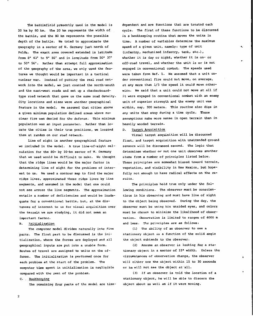
monitoring device will monitor 35 sensors in each
kilometer of the sensor band. Fig. 1 shows the
sensor layout for one nmnitor. The sensor range is
~ ’000 m—————+
+direction of expected
attack
Fig. 1. Sensor field monitored by one observer.
3
—
an input variable. We have been using ranges like
125 to 175 m for the detection of arnmred vehicles. ”
We have also been using a random range variation of
SbOUt *30% SmOng the various sensors in the field.
For realism, we say that something like 10 to 30% of
the sensors, randomly selected, do not
in a typical situation. These numbers
the capability of present-day sensors.
has a situation display map similar to
scribed in Ref. 2. The monitor merely
map display, designates a centroid for
work at all
are within
Each nmnitor
that de-
looks at his
the activated
sensors, and requests fire at the centroid.
E. Conventional Combat
Conventional combat is one of the weaker parts
of the mdel. The main purpose here was to indicate
the relative importance of conventional firepower
as opposed to nuclear firepower. A number of fac-
tors determine whether on not two opposing unita
will engage in conventional combat. The distance
between the unite and whether or not they can see
each other are two such factors. Equally important
is the military mission of the units. A nuclear
fire unit might be told to run when it sees the
enemy coming; other units might be told to fight
only if attacked; and others might be told to seek
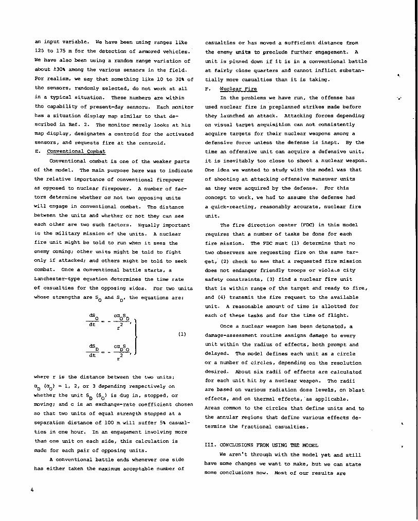
combat. Once a conventional battle starts, a
Manchester-type equation determines the time rate
of casualties for the opposing sides. For two unite
whose strengths are so and S~, the equations are:
&oCaosrl-—
T= 2’r
dsD CcisDO.—
T= 2’ 1r
(1)
where r is the distance between the two unita;
aD(ao) = 1, 2, or 3 depending respectively on
whether the unit SD (S.) is dug in, stopped, or
nwving; and c is an exchange-rate coefficient chosen
so that two units of equal strength stopped at a
separation distance of 100 m will suffer 5% casual-
ties in one hour. In an engagement involving more
than one unit on each side, this calculation is
made for each pair of opposing unite.
A conventional battle enda whenever one side
has either taken the maximum acceptable number of
casualties or has umved a sufficient distance from
the enemy units to preclude further engagement. A
unit is pinned down if it is in a conventional battle
at fairly close quarters and cannot inflict substan-
tially more casualties than it is taking.
F. Nuclear Fire
In the problems we have run, the offense has
used nuclear fire in preplanned strikes made before
they launched an attack. Attacking forces depending
on visual target acquisition can not insistently
acquire targets for their nuclear weapons among a
defensive force unless the defense is inept. By the
time an offensive unit can acquire a defensive unit,
it is inevitably too close to shoot a nuclear weapon.
One idea we wanted to study with the model was that
of shooting at attacking offensive maneuver unita
as they were acquired by the defense. For this
concept to work, we had to assume the defense had
a quick-reacting, reasonably accurate, nuclear fire
unit.
The fire direction center (FDC) in this model
reqUireS that a number of tasks be done for each
fire mission. The FDC must (1) determine that no
two observers are requesting fire on the same tar-
get, (2) check to see that a requested fire mission
does not endanger friendly troops or viola.e city
safety constraints, (3) find a nuclear fire unit
that is within range of the target and ready to fire,
and (4) transmit the fire request to the available
unit. A reasonable anmunt of time is allotted for
each of these taska and for the time of flight.
Once a nuclear weapon has been detonated, a
damage-assessment routine assigns damage to every
unit within the radius of effects, both prompt and
delayed. The model defines each unit as a circle
or a number of circles, depending on the resolution
desired. About six radii of effects are calculated
for each unit hit by a nuclear weapon. The radii
are based on various radiation dose levels, on blast
effects, and on thermal effects, “as applicable.
Areas common to the circles that define unita and to
the annular regions that define various effects de-
termine the fractional casualties.
III .
have
some
CONCLUSIONS FROM USING THE MODEL
We aren’t through with the model yet and still
some changes we want to make, but we can state
conclusions now. Most of our results are
●✌
✌✎●
4

1
probably already known to others, though perhaps in
different form. One of the first things we noticed
was the difficulty in finding out what had happened
in a battle without graphic output. A computer pro-
gram of this sort is seriously deficient without
graphic output. So much is going on that the time
required to check results with only printed output
is excessive. The problem might be c.mmpared to
trying to understand what has happened in a con-
ventional battle when you know only the casualties
and the coordinates of the individuals involved in
the battle as functions of time. Without a map
or similar aid to visualize what has happened, one
would be lost.
In our calculation where we are trying to
shoot at mobile offensive units as they are acquired
by the defense during the attack, the most important
parameter is time. From the time the defense first
sees attacking units until those units have closed
to within the minimum safe distance is a matter of
minutes. The defense must either deliver nuclear
fire on the attacking unita during this time or
fight the attacking unite conventionally, in which
case nuclear weapons would be limited in use to
rear-area targets and fixed targets. The times we
are talking about are somewhere between 5 and 15
minutes. About the only practical way our present-
day weapon systems can respond with sufficient
accuracy in this short time is if we fire them
from presurveyed positions into presurveyed target
areas. Presurveyed target areas and launch sites
are hardly acceptable in a mobile situation, howev-
er, so many people reject the idea of using nuclear
weapons against mobile maneuver elements. The only
obvious way around this problem is to have direct-
fire or terminally guided nuclear weapons. We
should note that this application against mobile
targets strongly influences weapon yield require-
ments as compared with something like tube artil-
lery. This is because the velocity of a nmving
unit is difficult to estimate and, over a 5-minute
period for instance, the error in target location
can be substantial.
Firing of nuclear weapons from presurveyed
positions involves another important time consid-
eration. If we assume the nuclear fire unit is
moved after each fire mission, the time required
to emplace the weapon in its new position and make
it ready to deliver accurate fire strongly affects
the number of fire units required to cover a given
area.
AS mentioned earlier, abeut the only way the
offense can use nuclear weapons is to shoot at areas
of activity and hope that defensive unita are in
that area. If the defense puta part of ita force
in strong bunkers, the area fire option becomes ex-
pensive for the offense. For instance, against
bunkers that will withstand (160-psi) loading, a
(1-Mt) weapon will only cover about 1 km2. The
cost to assure neutralization of a large area con-
taining bunkers is prohibitive.
Our study of unattended ground sensors used for
target acquisition was interesting. With the sensors
used as described earlier, we found that, against
armored unite, our target location errors were
comparable to those for visual observation. Sensors
decrease the certainty in locating any one part of
a target, but, since they do indicate the whole tar-
get, they give a good indication of its centroid.
The parameters that affect target location error are
sensor range, average variation in range, spacing
between sensors, and fraction of inoperative sensors.
IV. SOBIVXITINRS AND VARIABLES
A. Subroutines in the Model
In this section, we briefly explain the various
computational subroutines used in the model, but
make no effort to explain the output routines. Nor
will we explain the output variables when we later
cover the important variables. The prcqramming to
set up the output was simple, tedious, and not really
relevant to this report. The routines below are
grouped by task, but there is some overlap. Rou-.
tines that make no calls to other s&rOutines are
listed first in each group. The time-dependent rou-
tines presently run at the same time step but do not
have to.
(1) Initialization
SOBFQOTINE FOADNET
Given the variables DELSW, INS, DELNS,
and IEW, this routine loads the variables ~ADEW,
FOADNS, NOEWROA, AND NONSROA, which essentially de-
fine the road network.
SUBIKXITINE ‘TOWNINI
Given the road network, this routine
places on the roads those cities we use in our
5
—
population-avoidance calculation. The variables
‘TOWNX, ‘ICXVNY,TOWNR, and NOlY3WN define these cities.
To simplify computation, we handle the cities as
circles of various radii. For the area covered by
the problem, we have a list of the various city
radii and populations. Cities above the minimum
population are put on our road network in a random
fashion; the others are omitted from the computation.
SUBROUTINE INITIAL
This routine sets up a number of variables
for the line-of-sight calculation. By using the
ordering on the y coordinates that define the line
segments approximating the ridge lines, this routine
sets limits. These limits shorten the search needed
to determine if two points have line of sight. The
line-of-sight search is the most time-cmnsuming part
of the model.
SUBFLXITINE DEPILIY
This input routine deploys the offense
and the defense. The units must be placed in their
desired locations, and their destinations must be
defined. A number of variables are set in this
routine.
BULL
ThlS iS the control routine. A number of
input variables are defined in this routine, but
no real calculations tie made in it.
(2) Bookkeeping
LOGICAL FUNCTION ONROAD
Given the coordinates (x, y), ONROAD = .T.
if the point is on a road; otherwise, ONROAD = .F.
SUSlilXY1’INSVELCALC
Given the type of unit, whether it is day
or night, whether the unit is on or off a road, and
whether or not the unit is engaged in conventional
combat, this subroutine calculates the maximum speed
of the unit.
SUBF33UTINE UP(XX)FJI
For each time cycle, this routine updates
a number of variables for both the offense and de-
fense. All the visual target-acquisition variables
are cleared in this routine, and the variables as-
sociated with unit movement are updated. For each
time step while a unit is moving, a random varia-
tion of no greater than 20% is assigned to the
unit’s direction and speed. A number of nmvie
variables are also updated, and the variable DAY is
set in this routine. The routine uses VSLCALC and
ON ROAD .
(3) Target Acquisition
We will first cover the visual part of
target acquisition. The routines BINDATA and
RETRDAP set up data for visual target acquisition.
The routine IA3SIGHT makes the line-of-sight calcu-
lation. The routines OBSERVE and OBCONUF decide
whether one unit can see anobher if the two units
have line of sight.
SUBFf3~INE BINDATA
This routine divides the problem area inta
l-km squares. The defensive unite inside a l-km
square are stored together. The number of defensive
units is a maximum of NAXNOEL - 1 in any one square.
The number of storage locations used for each square
equals NAXNOEL. The first word of the list tells
how many units are in the square; the other words
are for unit numbers. If no defensive unit nrwes
during a cycle, this routine need not be called
the next cycle.
SUBIU)UTINE RSTRDAP
Given the unit number of an offensive
unit this subroutine finds those defensive units
within ILOS kilometers. The entry point INIRET
first calculates four indices that define a rectan-
crle of kilometer squares that must be searched.
Each succeeding call to RETRDAP calculates the unit
number of one defensive unit in the rectangle
defined by INIRST until they are exhausted. At thiS
point a zero is returned.
LOGICAL FUNCTION LOSIGHT
Given the unit numbers of an offensive
and a defensive unit, this routine calculates
whether or not there is a line segment approximating
a ridge that blocks the line of sight between the
two units. For most problems, the majority of
computer time is spent in this routine.
SUBlW3~INE OBSERVS
In this routine, each offensive unit is
checked against the defensive units within II.(X
kilometers to see if the units can observe one an-
other. First, we determine the maximum distance
over which a unit can be seen. We start by assum-
ing that one dug-in individual can be seen at up to
200 m and set dis max = 200. If the unit is not
dug in, we set dis max . 800. TO account for the
solid angle of the unit, we set dis max = dis max
unit strenqth. We next set dis max = dis max
● 2 if the unit has been observed or is moving.
.
..
6
We set dis max = dis max ● 2.5 if the unit is in
vehicles. Finally, we set dis max = dis max ● 1.5
if the unit is involved in conventional combat.
This part of the routine could perhaps be strength-
ened by taking into account the density of local
ground cover.
We also calculate what fraction of the distance
a 9iven observing ~it can see as conpared with a
unit in the same position under optimal circum-
stances. We start by taking into account the
strength of the obseming unit. Because of fatigue
and variations in eyesight, we say one individual
will be able, on the average, to see about 0.7 the
distance that a unit of say 25 people could see.
For larger units, there is little improvement. We
therefore set frac = minimum (1.0, 0.7 + 0.06*
unit etrength). Earlier we described how a mrxing
unit cannot see as well as a stationary unit. To
take this effe~~ti;~e~count, we set frac = frac*P
[1 - 0.5 (maximum unit speed)]. We say a unit in-
volved in conventional combat is going to be more
absorbed than a unit on the move. Hence, we set
frac = frac/3 if the unit ie involved in conven-
tional combat. Finally, we set frac = frac/2 if
it is night.
Given dis max for a unit being observed and
frac for a unit observing, we say that, if the
product (dis max) (frac) is greater than the dis-
tance between the two units, the observing unit can
see the other unit. Once it has been decided that
unit A has been observed, data are stored to indi-
cate the observation. Only the two opposition
units closest to A will store such data, wi~ one
exception: if A ie an offensive unit and the op-
posing side has an observer unit available, we
will carry that observer unit, whatever its posi-
tion, as one of the units observing A. Without
an observer unit acquiring an offensive unit, no
nuclear fire can be brought to bear on the unit.
We store an estimate for the centroid of unit
A. Computation of the error in this estimate is
described in our earlier section on target acqui-
sition. An estimated velocity vector is stored
for each acquired unit.
SUBROUTINE OBCONUP
For each defensive unit, this routine
calculates the numbers for dis max and frac de-
scribed in the OBSERVE writeup. These nunbers are
stored for use in OBSERVR.
Next, we cover those routines used to calculate
target acquisition from sensors.
REAL FUNCTION RANGESN
Given the indices needed to define a
specific sensor, this routine calculates the square
of the range for the specified sensor. This number
could be calculated once at the start of the prob-
lem and stored, but we calculate it each time it 1S
needed to save storage. The range of a sensor has
a random variation that is a function of the indices
of the sensor. For this variation to remain mn-
stant throughout the problem? we compute a random
number that is a function only of the indices needed
to specify a censor.
SUBROUTINE TXTYFL
Given the indices of an activated sensor
mcnitored by a specified operator, this subroutine
finds the other activated sensors monitored by the
same operator that can be reached by following a
continuous path of activated sensors. This gives
the approximate area occupied by one unit. Once the
sensors defining a single target have been found,
the centroid ia calculated. No information passes
from one monitor to the next. The fire direction
center must decide if two monitors are seeing the
same unit.
REAL I?UNCX’IONYYY
Given a specific row and a specific mcn-
iter, this routine calculates the y coordinate of
the row of sensors.
SUBFC)UTINE CLOS
Given the cmrdinates of an armored ve-
hicle, this routine, along with INDXRNG and RANGESN,
calculates what sensors are activated and decides
which operators monitoring the field, if any, might
get a sensor reading.
SUB133UTINE INDXPJIG
Given a point (x, y) and an operator num-
ber, this routine activates the sensors monitored
by the specified operator within range of the mint
(x, y). The y coordinate is given relative to the
start of the sensor field.
SUBROUTINE 5EN51NT
Given the ou$put of the routine TXTYPL,
this routine sets
execute a nuclear
up the information needed to
fire mission.
7
—
(4) Conventional Action
SUBIKXITINE CASCOBA
This routine calculates the casualties
from conventional battles; it also calculates wheth-
er or not a unit is pinned down. For lack of a smre
precise measure, we say a maneuver unit’s fighting
ability is proportional to its manpower. The basic
equations for determining conventional casualties
and whether or not a unit is pinned down were de-
scribed earlier.
SUBROUTINE ENDCOBA
This routine removes units from conven-
tional battle when their casualties have made them
ineffective, when they are sufficiently separated
from enemy units involved in the battle, or when
they have lost line of sight with enemy unite in-
volved in the battle. Each time a unit is removed
from battle, the routine provides a printed output.
The routine ends conventional battles whenever all
the unite on one side are removed from the battle.
The routine calls ENDBAT, REPOS’10, REPOSTD, PUR3FFU,
and PUADEFU.
SUBFKXJTINE ENDBAT
Given the number of a battle that has
ended, this routine restores the variables UNENOFF,
UNENDEF, NOUNDFG, and NOUNOFE so the given battle
is removed from the computation. This routine calls
SEPOSTO and REPOSTD and has the entry points PURCIFFU
and PURDEFU. Given a unit number, these entry pointa
purge an offensive unit or a defensive unit from
the calculation. The units are assumed to be in-
effective at that point.
SUBROUTINE REPOS’M
This routine is called when an offensive
unit involved in conventional battle breaks off
the engagement but remains effective. The routine,
which calls ONROAD, calculates the new posture for
the unit. The routine has a second entry point,
REPOSTD, which makes the same calculation for
defensive units.
SUBROUTINE INICOND
This routine, along with FUENGAG, mn-
trols the mnventional actions that defensive
unite take with respect to the offensive units
acquired. These actions include starting an am-
bush, starting a conventional battle, withdrawing
action depends on the mission of the defensive unit,
the relative strengths of the defensive unit and the
acquired offensive unit, the distance between them,
and the direction the offensive unit is moving
(toward or away from the defensive unit). These
decisions must be programmed for each type of unit.
Decisions on conventional action are presently made
on a local basis without reference to the whole
battle area, in line with our view that the defense
will want to maneuver mostly on the basis of local
conditions.
SUBROLFI!INEINICDNO
This routine makes the same calculations
for the offense that INICOND and FUENGAG make for
the defense.
SUBROUTINE NEXTBAT
Any time a unit starts a conventional
battle with another unit, this routine handles the
bookkeeping. It also handles any ambushes. The
ambush logic works as follows. Suppose unit A ac-
quires unit B and unit B is not in a defensive po-
sition. Unit A can ambush unit B if unit A is not
already involved in conventional combat and unit B
has not acquired unit A. If unit A ambushes unit
B during the day and the units are separated by
150 m or less, we say that half the individuals in
unit A will each inflict a casualty on unit B in
the opening burst of fire, before unit B can take
cover. We assume here that unit B is at least
comparable in size to unit A. If unit B is much
smaller, it will be destroyed and pose no further
problem. At 150 m, nearly everyone should be able
to hit an unwarned target; but, for a number of
reasons, we say about half the individuals in unit
A will not be in a position to fire. If the ambush
occurs at night, the equivalent effective distance
must be divided by 2. If the ambush accurs at some
distance d > 150 m, the casualties drop by the fac-
150 2tor (T) . If an ambush renders a unit ineffec-
tive for combat, NEXTBA72 removes that unit from the
calculation.
REAL FUNC1’ION DISTMIN
Given an offensive unit M acquired by a
defensive unit I, this routine calculates an es-
timate of how close unit M will come to unit I,
if unit M continues on its observed course.
‘4
.,.
b
to a new position, and hiding in a position while
waiting for the enemy to bypass. The choice of
8

SUBROU1’INS FINPTCL
Given coordinates (x, y) end the number of
an appmxi!nate ridge line, this routine calculates
the distance from the point (x, y) to the Closest
point on the line segment representing the ridge
line and calculates that closest point on the line
segment. Finally, it calculates the closest point
to point (x, y) that is 100 m from the line segment
on the side away from point (x, y) . This routine is
used in conjunction with LOSSAFD to find cover for
defeneive unite from attacking unite. The routine
also has the entry point FINMIND. Given a point
(x, y) and the number of an approximate ridge line,
this entry point calculates the shortest distance
from the point (x, y) to the line extended from the
given line segment.
SUBROUTINE LOSSAFD
Given the locations of an offensive unit
and a defensive unit, this routine finds the closest
approximate ridge line to the defensive unit that
blocks line of sight to the offensive unit. This
routine uses FINPTCL.
SUBFSXITINE MOVEDEF
This routine sets up the path a defensive
unit is to take when it moves for some reason. For
instance, each time a nuclear fire unit is given a
fire mission, it moves to a new location. This move
is made in a random manner. Thus, if the unit is on
a north-south road, the decision to go north or
south is made by a random number generator. Nhen
the unit comes to an intersection, the direction it
takes is again determined by a random number gen-
erator. Finally, the distance it moves along the
chosen route is also determined in a random manner.
The above choices are all subject to restrictions
that the unit must stay inside the problem area
and within range of the defensive line.
(5) Nuclear Fire
REAL FUNC1’ION PSIRAD
Given a yield and a pressure in psi, this
routine calculates the distance at which the hori-
zontal component of peak pressure matches the speci-
fied pressure. The routine merely does a linear
interpolation for a l-kt weapon by using data given
in Ref. 3. The result is then multiplied by the
cube root of the yield.
REAL FUNCTION FISRAD
Given a yield and a radiation dose, this
routine calculates the maximum distance at which a
fission device will provide the specified dose.
The routine assumes the dose at a fixed distance is
linear with yield. By dividing the input dose by
the input yield, we get a scaled dose (dose per
kiloton) . By using l-kt data, we then calculate
the distance at which we will get the scaled dose
with our input yield. This last calculation is
simply a logarithmic interpolation from a series
of data points.
The routine also has an entry point, FISDOS,
that calculates tie radiation dose as a function
of yield and distance to the zero point. The
calculation is the same as above except that the
interpolation is inverted.
REAL FUNCTION THERMDI
Given a yield, this routine calculates
the distance at which individuals would get first-
or second-degree burns if skies were clear. The
routine uses data from Ref. 3.
REAL FUNCTION OVERTRN
Given the yield, this routine calculates
the distance at which weapon blast will overturn
an armored vehicle. The data used here came from
Ref. 3 and are assumed to be the same as for earth-
moving equipment.
REAL FUNCTION CIRCCAL
Given two circles Cl and C2 with radii
R1 and R2 and the distance d from center to center,
this routine calculates the fractional area of
Cl contained in C2.
SUBROUTINE FRACCOV
Given the radii of effects against a
specified unit for the various classes of radiation
doses and for blast damage and thermal damage, given
the distsnce from the zero point to the specified
unit, and given the radius of the unit, this routine
computes the fractions of prompt casualties and of
various classes of delayed casualties. Casualties
are assessed on an area basis. This routine uses
CIRCCAL .
REAL FUNCTION EFFE~C
This routine calculates radii of effects
of nuclear weapons for different types of unite in
differing postures. It provides the logic to
9
account for a unit’s hardness before it calls other
routines to make the desired calculation. This rou-
tine uses PSIRAD, FISSAD, THERMDI, and OVERTRN.
SDBIWNTINE DELAYCA
For each offensive and defensive unit,
this routine calculates any delayed casualties. The
casualties in each class are assessed linearly in
time. For instance, if ten class 2 casualties are
to become incapacitated in ten days, this routine
will assess one casualty per day for ten days. If
at any time the unit becomes ineffective because of
delayed casualties, this routine purges the unit
from the calculation. In the problems we have run
so far, delayed casualties have not had an important
effect.
SUBROUTINE NUCIMPT
Given a nuclear shot, a predicted zero
point, and a CEP, this routine computes an actual
zero point and assigns casualties to any units that
receive prompt casualties from the weapon. If the
nuclear shot has terminal guidance, the routine cam-
putes a final predicted zero point. This routine
purges from the calculation any units whose prompt
nuclear casualties are sufficient to render the unit
ineffective. The routine computes the radiation
dose at the center of each unit to keep track of
aPPrOxlmate Cumulative dose. The routine sets up
the data for delayed casualties. Finally, the rou-
tine sets up a number of variables for output prints
and plots. The routine uses EFFECTC, FRACCOV,
FISCOS, PUlW3FFU, PURDEFU, THERMDI, FISRAD, and
PSIRAD.
REAL FDNCI!ION FRNDSFO
Given a yiel&, a predicted zero point,
and a specified offensive unit, one can calculate
the unit’s distance from the zero point minus the
minimum safe distance. This routine calculates the
smallest such number anmng all offensive units.
If the number is negative, the shot would endanger
offensive units. This routine has the entry point
FRNDSFD, which makes the same calculation for de-
fensive units. Finally, the routine has the entry
point CITYSAF, which,given a yield, will calculate
a minimum safe distance for cities. Given next a
zero point, this routine calculates the minimum
distance, among all cities, to the circle defined
by minimum safe distance from the zero point.
In each of the above calculation, one computes the
distance that a zero point can be moved before a
safety criterion is violated.
INTEGER FUNCTION FINFUND
Given the coordinates (x,Y) , this routine
finds a nuclear fire unit that is within range of
the point and ready to fire. Starting from a random
point, the routine searches the list of fire units.
If a unit is not available to fire at the target,
a zero is returned for the unit number.
SUSIKWTINE FRMSNDF
This routine, along with FINFUND, FFNDSFD,
and CITYSAF, is the model analog of the fire direc-
tion center. After the appropriate time delay fol-
lowing target acquisition, this routine looks at all
fire-mission requests, checks for troop and city
safety, checks to make sure that no two observers are
requesting fire on the same target, assigns an
available nuclear fire unit (if one exists within
range of the target) , and sets UP the time delays
appropriate to carrying out the fire mission.
This routine also seta up the fire missions for
execution in conjunction with unattended ground
sensors. The safety checks are not needed since
they are implicit in the location of the sensors.
B. Variables in the Model
When we were programming the model, we decided
to store information as it was generated and use it
at a convenient time in the calculation. As a re-
sult, many variables carry information from one rOu-
tine to the next, when the calculation could have
been done in one step. This approach makes the
programming easier to prepare and much easier to
change but uses more storage.
Nhen a variable refers to, say, a defensive
unit, there is usually a corresponding variable
for the offensive unit. Rather than list both,
we list only the defensive variables. The unit
numbers given below refer to logical unite inside
the computer model. One milita~ unit may have more
than one logical unit. For instance, each tank of
a tank company may be a logical unit, or the whole
company may be one logical unit, depending on the
resolution desired.
XDEF(I) is the x inordinate of the Itb defensive
unit.
YDEF(I) is the y coordinate of the Itb defensive
unit.
NOUNITD is the number of defensive units at the
b
10
f
start of the problem.
VDEF(I) is the speed of the Ith defensive unit.
[UXDEF(I), ~DEF(I)l iS the Unit velocitY vector
for the Itb defensive unit.
The pairs of variables [xlDEF(I), YIDEF(I)I,
[X2DEF(I), Y2DEF(I)1, and [X3DEF(I), Y3DEF(I)I de-
fine paths of travel for the Itb defensive unit.
The unit is first to go to point [XIDEF(I),
Y1OEF(I)I, then b [X2DEF(I), Y2DEF(I)I, and finallY
ti [X3DEF(I), Y3113F(1)I. These variables are used
if a unit has multiple objectives or are used to de-
fine alternative paths of travel if the planned path
of travel is blocked. pairs of zexns are used to
indicate no path is defined.
UNSTRID(I) is the strength of defensive unit I at
the start of the problem. UNSTRD(I) is the strength
of defensive unit I at later timee. Whenever the
fraction UNSTRD(I)/UNSTRID(I) goes below a Certain
level, the unit is defeated.
RADDEF(I) is the radius of defensive unit I. Each
unit is logically thought of as a circle.
TYPEDND(I) is an integer defining tie function Of
defensive unit I. At present, TYPEUND = 1 is a nu-
clear fire unit, TYPEUND = 2 is a forward obeerver
unit, TYPEDND = 3 is an infantry unit assigned to
protect a forward observer unit, TYPEUND = 4 is a
local militia unit, TYPEUND = 11 is a mechanized
infantry unit, and TYPEUND = 12 is a tank unit.
The variable is used to assess nuclear casualties,
to determine speed, and to determine what conven-
tional action a unit takes under given circumstances.
POSTURD(I) is an integer defining the posture of
the Ith defensive unit. POSTURD = - 1 means the
unit is ineffective, POSTURD = O means the unit is
stopped and dug in, POSTURD = 1 means the unit is
rmving cross-country at full speed, POSTURD = 2
means the unit is moving down a road, POSTURD = 3
means the unit is reeving cross-country slowly with
maximum use of covers, POSTURD = 4 means the unit
is stopped and in conventional combat, POSTURD = 5
means the unit is reeving and in conventional combat,
and POSTURD = 6 means the unit is dug in and in con-
ventional conbat. POSTURD and TYPEUND have essen-
tially unlimited possibilities for definitions.
TMPODEF(I) is the length of time that defensive ~it
I has been in its present posture.
The model carries up to three different classes
of delayed casualties, each with a different time to
incapacitation. SIDEF (I), 521X3F(I), and S3DEF(1)
are the numbers of casualties for the Ith defensive
unit in each of the three classes.
TIDEF(I) , T2DEF(I) , and T3D5F(I) are the timee tO
incapacitation for the three corresponding classes
of casualties.
UN1OBSD(I) is the unit number of the closest of-
feneive unit that has defensive unit I visually
acquired at the present time. UN20BSD(I) is the
unit number of the second-closest offensive unit
that has defensive unit I visually acquired at the
present time.
TMCOOBD(I) is the length of time that the offense
has continuously observed defensive unit I visually.
TMLAOBD(I) is the last time defensive unit I was
visually observed.
[XEDEF(I), YEDEF(I)] is the set of (x, y) coordinates
for the center of defensive unit I as estimated by
the offense the last time the unit was visually ob-
served.
[XTDSF(I), YTDEF(I)] is the velOcity vectOr Of de-
fensive unit I as estimated by the offense.
(33NOBSD(I) tells how far defensive unit I is
visible under optimal circumstances. It corresponds
to dis ma% in the previous section on OBSERVE.
CON~BS(I) tells the fractiOn of the distance that
defensive unit I can see as compared with a unit in
the same position under optimal circumstances.
This corresponds to frac in the previous section
on OBSERVE.
BSTHDDF(I) is the blast pressure in psi needed to
destroy defensive unit I.
RADHDDF(I) is the radiation transmission factor
for defensive unit X. This factor can vary with
the posture of the unit.
UNIBOBD(I) is the unit number of the closest of-
fensive unit that defensive unit I is observing.
DIBOBD(I) is the estimated distance between offen-
sive unit UNIBOBD (I) and defensive unit I.
D2BOBD(I) and DN2BoBD(I) carry the same distance
information for the second closest unit.
DMAXDBF(I) and DMINDEF(I) are two variables used
in the OBSERVE subroutine that temporarily carry
the distances DIBOBD(I) and D2BOBD(I)-
CEPDSF is the CSP of the defensive nuclear fire
units if they are not range-dependent and use only
one type of fire unit.
INUCDEF(I) is the number of nuclear weapons expended
11
—
by defensive unit I. This variable is important
only for nuclear-capable units.
RADLVLD(I) is the radiation dose received at the
center of defensive unit I. This variable is ueed
nmstly to monitor friendly casualties.
‘IM’IOMCD(I)is used with forward observer unite that
provide terminal guidance to nuclear fire. This
variable tells how long it will be before the equip-
ment used by defensive unit I for terminal guidance
is free for another mission.
EXCOEF corresponds to the c we used back in Eq. (1).
TMTODC3 is an input variable. It tells the maximum
time that delayed casualties in class 3 will live.
TM1’0DC4 carries the same information as ‘ITYIODC3,
except it is for class 4.
TMTODR is an input variable that tells the maximum
time to death for persons receiving a fatal radia-
tion dose.
TIMEINT is the time of day in minutes that the
problem started; 6 a.m. is assumed to be zero.
TIME contains the problem time in minutes.
IELT is the time step between cycles and may vary
during the problem.
DAY is a logical variable indicating day or night.
DAY = .T. implies daytime and DAY = .F. implies
nightime.
At any given time,’ there may be up to 20 nu-
clear shots being fired. Between the time the re-
quest for nuclear fire goes to the fire unit and
the time the shot detonates, information on the
shot is carried in the following variables. The
ordering on ~e index J merely indicates the order
in which fire-mission requests have gone to the
fire units. It has no importance.
NOSTRIK is the number of nuclear shots being exe-
cuted.
YIELD(J) is the yield of the Jth shot.
UNFRDAT(J) is the unit number of the target of the
Jth shot. The number is negative if the target is
a defensive unit and positive if the target is an
offensive unit. The number is carried so that, if
the shot has terminal guidance, the target data can
be updated.
[PREDX(J), PREDY(J)I is the predicted ground zero
for the Jth shot.
TRANMAX(J) is used with terminal guidance as a
sefety check. Once a shot has been requested and
a predicted ground zero has been specified for the
Jth shot, the terminal guidance can divert the shot
from the predicted ground zero by, at most, the dis-
tance TRANMAX(J).
TMTOIMP(J) is the time to zero point for the Jth shot.
CEPNUC(J) is the CEP for the Jtb shot.
The following input variables relate to nuclear
missions fired by the defense.
TREXFRM is the time required for a nuclear fire unit
to execute a mission after it receives a fire-
mission request. This time assumes the unit is
ready. With an artillery piece, for instance,
this would be the time required to load the round,
load the powder charge, point the tube, and pull
the lanyard.
YIELDDF(J) for J = 1, 2, 3, 4, 5 iS the Set Of
yields available for the defensive units. For the
problems run so far, only one yield has been used.
TREBGNM is the time a defensive nuclear fire unit
requires to get ready to deliver accurate fire af-
ter it arrives at a new presurveyed position. For
an artillery piece, this would be the time required
to dig in the spade and lay the gun.
RANG!3 is the maximum range for a defensive nuclear
fire unit.
RANGEMN is the minimum range for a defensive nucle-
ar fire unit.
‘lUF is the time of flight at maximum range for a
defensive nuclear fire unit.
TMcXX4MD is the time required for the defensive FDC
to receive afire mission, make any safety checks,
decide whether or not the mission should be fired,
and forward the request to an available nuclear
fire unit.
SMAI..OUNis the smallest visually acquired offense
unit that will be a nuclear target for the defense.
In reality, the defense would have to guess at the
size of a unit it acquired. For sensor-acquired
offensive units, the defense can only look at the
number of sensors that signal an intrusion.
PSIMAXD is the maximum blast overpressure used in
specifying trcep safety requirements for the
defense.
RADNAXD is the prompt radiation dose used in
specifying troop safety requirements for the de-
fense.
RADEMGD is the prompt radiation dose used in
specifying troop safety requirements for the
8
7
12
defense in emergency situations.
PSINAX is the maximum blast pressure allowed on a
safe city. WW is the maximum prompt radiation
dose allowed on a safe city.
The following variables are used to describe
the road network.
NONSI@A is the number of north-south roads in the
problem.
R3ADNS(J) is the x coordinate of the Jth north-
south road.
NOEWFQA is the number of east-west roads in the
problem.
ROADEW(J) is the y coordinate of the Jth east-west
road.
DELNS is an input specifying the spacing between
north-south roads.
DELEW is an input specifying the spacing between
east-west roads.
The following variables are used in the con-
ventional-combat part of the mode.
NAXNOBA is the maximum number of conventional
battles allowed to go on at any one time (a storage
limitation).
NOBATTL is the number of battles in progress.
NOUNDFE(J) is the number of defensive unita en-
gaged in the Jth battle. The battles are numbered
sequentially in the same order as they start. My
battle that is stopped is remcved from the list.
O < J < NOBATTL.Note: _ _
UNENDEF(J, K) is the unit number of the K* defen-
sive unit involved in the Jth battle. Note:
()~K~NOIJND~(J). my unit no longer in the bat-
tle is remved from the list.
MAXELEN is the maximum number of elements on either
the defense or the offense that are allowed to be-
come engaged in one conventional battle (a storage-
size limitation) .
STSMIND is the fractional level of strength (an
input variable) at which a defensive unit becOmes
ineffective. In most real situations the mental
attitude of a unit is nmre important that its
physical situation. Unfortunately, we know of no
way to model the mental attitude.
The following input variables are used in as-
sessing damage from nuclear weapons.
The model uses four different prompt radiation
dosea : C2DOSE, C3CK)SE, C4DDSE, and LETiiCOS. We
presently use C2LY3SE as the minimum dose needed for
immediate casualties. The other three levels of
radiation dose are used for delayed casualties.
EARBFST is the amount of blast pressure in psi
needed to rupture eardrums. We assume this blast
pressure to cause instantaneous casualties anmn9
personnel who are exposed or in foxholes.
TRFCAPC is the transmission factor for an APC.
TRJ?CTK is the transmission factor for tanks.
Tlc?CFOX is the transmission factor for foxholes.
The following miscellaneous variables are
related to problem size.
IIOS is the maximum distance in kilometers that a
person can see.
-OEL is the maximum number of defensive unita
allowed in a square kilometer (a storage limitation) .
INS is the distance in kilometers that the problem
covers in the y direction.
IEW is the distance in kilometers that the problem
covers in the x direction.
CONDISS is the square of the maximum distance at
which effective conventional combat can occur.
The following variables are used in computing
targets on the basis of outputs frOm unattended
ground sensors.
SENSOR (I, J, K) is a logical variable. In our sen-
sor field, we say one operator monitors the sensors
on 1 km of front. For each sensor in the field,
there is at least one set of indices I, J, ad K for
the variable SENSOR. The index K tells what opera-
tor is
J tell
of the
SENSOR
sensor
SENSOR
sensor
monitoring the sensor, and the indices I and
the location of the sensor inside that part
field monitored by operatir K.
(I, J, K) = .T. implies that the specified
is indicating an intrusion.
(I, J, K) = .F. implies that the specific
is not indicating an intrusion. If a specif-
ic sensor is not functional, it is always false.
Note: the sensors on a boundary between two opera-
tors are monitored by both operators.
CONSENS (I, J) is a logic variable used to calculate
how many tripped sensors in a field monitored by
one operator are neighbors of one another. A group
of tripped sensors is used to indicate the approxi-
mate outline of one unit.
TsIUC) is a 109ic vari~le.
TS1(K) = .F. indicates monitor K has no targeta
acquired by the sensor field.
TS1(K) = .T. implies monitor K has a target and
13
—

the coordinates are stored in the variables
[TX1 (K) , ml (K) 1. These coordinates are merely the
centroid of a connected group of sensors that have
been tripped. The model can store three separate
targets for each operator.
The other variables used are TS2(K), TX2(lC), TY2(K),
TS3(K), Tx3(K), and TY3(K).
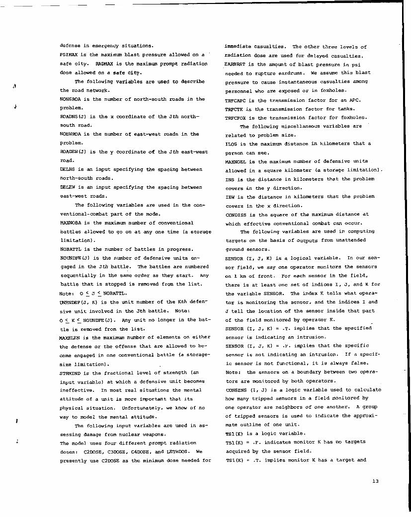
IROW is the number of rows of sensors. In Fig. 1,
IFOW = 7.
JCOL is the number of columns of sensors monitored
by one operator. In Fig. 1 JCOL = 5.
DXSENS is the x distance between sensors.
DYSENS is the y distance between sensors.
SENSRNG is the average range (an input variable) at
which a sensor will pick up an armored vehicle.
Each sensor actually has a range that is chosen at
random between SENSl?r4G- 1/2 VM and SENSPNG + 1/2
VARI . VARI is another input variable indicating
the variation.
The following input variables are used to ap-
proximate the geography of the area of interest.
POPMIN is the minimum population needed to establish
a Ppulation center as a safe city. By a safe city,
we mean an area in which the defense will not use
nuclear weapons in a way that causes nmre than,say,
light damage. The citiee are assumed to be circular.
NOICIWN is the number of safe cities in the defensive
area.
[’IOWNX(I)J TOwNy(I)l is the set Of c~rdinates for
the center of the Itb safe city.
TOWNR(I) is the radius of the Ith safe city.
NOLOSBL is the number of important ridge lines in
the problem area. At present, NOIOSBL = 37.
[xlIOS(I), YILOS(I)], and [X2LOS(L), Y21.OS(I)] are
the end points of the line segments used to approxi-
mate the ridge lines.
REFERSNCSS
1.
2.
3.
Staff Officer’s Field Manual Org anization,
Technical and Logistical Data, Department of the
?irmy Field Manual, FM 101-10-1 (July 1971),pp. 2-11.
Surveillance, Target Acquisition and Night
Observation (STANO) Operations, Department ofthe Army Field Manual, FM 31-100 (May 1971),pp. B118-B119.
Samuel Glasstone, The Effects of NuclearWeapons. United States Atomic Energy Commission,April 1962, pp. 137-139, P. 573, PP. ~74-~75.
7
;
c
30:120(90)
14
Recommended