Chapter 6
COMPUTATION OF RESIDUE CURVES USING
MATHEMATICA®
AND MATLAB®
Housam Binous* Chemical engineering Department
King Fahd University, Petroleum and Minerals,
Dhahran, Saudi Arabia
ABSTRACT
The Author presents a teaching technique used successfully in an undergraduate
course to seniors at The National Institute of Applied Sciences and Technology (INSAT)
in Tunis, Tunisia. The present paper details the computational aspects needed to obtain
residue curves (RCs) for a binary and various ternary systems using Mathematica® and
MATLAB®, which are taught in Tunisia. The first mixture studied is composed of
ethanol Ŕ isopropanol. A ternary ideal mixture composed of benzene Ŕ toluene Ŕ p-xylene
is treated next. A non- ideal ternary mixture (ethanol Ŕ water Ŕ ethylene glycol), using the
Wilson model to predict liquid-phase activity coefficients, is also presented. Finally, a
case, where both high pressure effect and deviation from ideal behavior in the liquid
phase must be considered, using the Soave - Redlich - Kwong (SRK) equation of state
(EOS) and the Wilson model, respectively, is studied. This final mixture contains
acetone, chloroform and methanol. All problems are solved using the built-in
Mathematica® and MATLAB® commands NDSolve and ode15s. The author concludes
with insight to using residue curves (RCs) in order to teach distillation with the help of
computer software such as Mathematica® and MATLAB®.
Keywords: Residue Curve, distillation, Mathematica®, MATLAB®.
In: Computer Simulations
Editors: Boris Nemanjic and Navenka Svetozar
ISBN: 978-1-62257-580-0
c© 2013 Nova Science Publishers, Inc.
The exclusive license for this PDF is limited to personal website use only. No part of this digital document may be reproduced, stored in a retrieval system or transmitted commercially in any form or by any means. The publisher has taken reasonable care in the preparation of this digital document, but makes no expressed or implied warranty of any kind and assumes no responsibility for any errors or omissions. No liability is assumed for incidental or consequential damages in connection with or arising out of information contained herein. This digital document is sold with the clear understanding that the publisher is not engaged in rendering legal, medical or any other professional services.

Housam Binous 162
NOMENCLATURE
P : total pressure (bar)
Pc,i: critical pressure (bar)
Pr,i: reduced pressure
𝑃𝑖 : partial pressure (bar)
𝑃𝑖𝑠𝑎𝑡 : vapor pressure (bar)
t : time (hr)
T : temperature (K )
Tc,i:: critical temperature (Kelvin)
Tr,i: reduced temperature
x : liquid composition (mole fraction)
y : vapor composition (mole fraction)
Z: compressibility factor
Greek Letters
φ: fugacity coefficient
γ: activity coefficient
ξ: warped time
acentric factor
INTRODUCTION
Distillation is the most ubiquitous unit operation in the chemical industry. Thus, a good
grasp of this separation method is essential both to chemical engineering students and
professionals. By looking at the composition of the still during a simple batch distillation, one
can plot a residue curve and gain insight to the product composition (distillate and bottom) of
a particular distillation column. Indeed, for a ternary system for example, the location of the
bottom and distillate are near both the residue curve and the distillation curve. One can plot
what is called a residue curve map (RCM) by selecting different initial compositions in the
still and plotting the corresponding residue curves. Another useful feature of residue curve
maps is that the azeotropes appear as extremes (saddle points, stable nodes and unstable
nodes; see Figure 1).
Figure 1.Extreme points for the RCM.
Thus, by computing residue curve maps, one finds the location of all azeotropes
naturally. Sometimes RCMs show peculiar features such as distillation boundaries. This
phenomenon leads to interesting conclusions about the feasibility of any distillation scheme.

Computation of Residue Curves Using Mathematica® and MATLAB® 163
Indeed, a distillation boundary cannot usually be crossed by a single column unless it is
curved. In the present paper, the author attempts to provide students and professional with
details about the programming techniques used to compute RCs with the help of modern
scientific computing tools such as Mathematica®
and MATLAB®. The first part of the paper
gives the governing equations that one has to solve in order to compute RCs. A short
description of the rules that allow vapor-liquid prediction, for ideal and non-ideal liquid and
gas-phase behaviors, is given next. The first problem studied is a binary mixture composed of
ethanol Ŕ isopropanol. The entire commented code, given in Appendixes 1 and 2, is described
for an ideal ternary mixture composed of benzene Ŕ toluene Ŕ p-xylene both for
Mathematica® and MATLAB®. A ternary system is then studied. The corresponding mixture
is composed ethanol Ŕ water Ŕ ethylene glycol. This system is useful for the production of
anhydrous ethanol using extractive distillation. In order to show how one performs
calculation of RCs when there is deviation from ideal behavior in both the liquid and gas-
phases, results concerning a mixture of chloroform Ŕ acetone Ŕ methanol are provided. In the
last section, the author concludes by sharing his experience teaching distillation to
undergraduate students at the National Institute of Applied Sciences and Technology
(INSAT) in Tunis, Tunisia.
GOVERNING EQUATIONS FOR RESIDUE CURVES
A residue curve is obtained by solving the following equations:
𝑑𝑥𝑖
𝑑𝜉= 𝑥𝑖 − 𝑦𝑖 for i=1 to Nc (1)
where 𝑥𝑖 and 𝑦𝑖 are the liquid mole fraction of component i in the still and the equilibrium
vapor mole fraction. ξ is the warped time defined by: 𝑑𝜉 =𝑉
𝐻 𝑑𝑡 where t is the clock time, H
is the molar hold-up in the still and V is the vapor boil up rate. These equations are obtained
from the overall material balance and the (Nc -1) independent component balances written for
the simple batch distillation scheme shown in Figure 2. A full derivation of these equations is
given by Doherty and Malone (2001).
For binary mixtures where the equilibrium behavior is modeled by the empirical relation:
𝑦 =𝑎 𝑥
1+ 𝑎−1 𝑥+ 𝑏 𝑥 1 − 𝑥 , (2)
the RCs are given by the following implicit equation:
𝜉 =1
𝑎−1+𝑏 𝑙𝑛
𝑥0 1−𝑥
𝑥 1−𝑥0 +
𝑎−1 2
𝑎−1+𝑏 𝑎−1+𝑎 𝑏 𝑙𝑛
1−𝑥 𝑎−1+𝑏 1+ 𝑎−1 𝑥0
1−𝑥0 𝑎−1+𝑏 1+ 𝑎−1 𝑥 . (3)
This equation is obtained by using Equations (1) and (2), the method of partial fractions
and separation of variables.

Housam Binous 164
It is clear from Equation (1) that good vapor-liquid equilibrium prediction will be
necessary in order to compute RCs. The next section presents extensive details about this
important matter, which is ubiquitous in chemical separation science.
Figure 2. Batch dstillation still.
VAPOR-LIQUID EQUILIBRIUM PREDICTION
Vapor pressure, a function of temperature only, is given by empirical equations such as
the Antoine equation:
𝑙𝑜𝑔 𝑃𝑖𝑠𝑎𝑡 = 𝐴𝑖 −
𝐵𝑖
𝐶𝑖+𝑇 , (4)
and the Modified Antoine equation:
𝑙𝑛 𝑃𝑖𝑠𝑎𝑡 = 𝐴𝑖 +
𝐵𝑖
𝐶𝑖+𝑇+ 𝐷𝑖 𝑙𝑛 𝑇 + 𝐸𝑖 𝑇
𝐹𝑖 , (5)
where 𝐴𝑖 , 𝐵𝑖 , 𝐶𝑖 , 𝐷𝑖 , 𝐸𝑖 and 𝐹𝑖 are the constants, which depend on component i.
If the pressure effects cannot be neglected, one has to use Eq. (6) to model vapor-liquid
behavior:
𝜑𝑖 𝑦𝑖 𝑃 = 𝑥𝑖 𝑃𝑖𝑠𝑎𝑡 𝛾𝑖, (6)
where 𝜑𝑖 is the gas-phase fugacity coefficient always obtained from an EOS such as the
Soave-Redlich-Kwong equation of state and 𝛾𝑖 is the activity coefficient given by the widely

Computation of Residue Curves Using Mathematica® and MATLAB® 165
used Wilson model. This model allows good prediction of vapor-liquid data when one deals
with mixtures that do not present demixtion into two liquid phases such as immiscible and
partially miscible mixtures. The Wilson model (Wilson, 1964 and Sandler, 1999) is given by
the following equations:
𝑙𝑛 𝛾𝑘 = −𝑙𝑛 𝑥𝑗 𝐴𝑘𝑗𝑁𝑐𝑗=1 + 1 −
𝑥𝑖 𝐴𝑖𝑘
𝑥𝑗 𝐴𝑖𝑗𝑁𝑐𝑗=1
𝑁𝑐𝑖=1 (7)
In Equation (7), 𝐴𝑖𝑗 is the binary interaction parameter, which depends on the molar
volumes (𝑣𝑖 and 𝑣𝑗 ) and the energy terms 𝜆𝑖𝑖 and 𝜆𝑖𝑗 ,
𝐴𝑖𝑗 =𝑣𝑗
𝑣𝑖𝑒𝑥𝑝 −
𝜆𝑖𝑗−𝜆𝑖𝑖
𝑅 𝑇 . (8)
The fugacity coefficient in the gas-phase is given by the following equation (Sandler,
1999 and Soave 1972):
𝜑𝑖 = 𝑒𝑥𝑝 𝑍 − 1 𝐵𝑖
𝐵− 𝑙𝑛 𝑍 − 𝐵 −
𝐴
𝐵
2 𝐴𝑖0.5
𝐴0.5 −𝐵𝑖
𝐵 𝑙𝑛
𝑍+𝐵
𝑍 (9)
In Equation (9), Z is the compressibility factor, which is a solution of the cubic equation
(Sandler, 1999 and Soave 1972):
𝑍3 − 𝑍2 + 𝑍 𝐴 − 𝐵 − 𝐵2 − 𝐴 𝐵 = 0 (10)
Constants 𝐴𝑖 ,𝐵𝑖 ,𝐴 and 𝐵 depend on the reduced pressure (𝑃𝑟 =𝑃
𝑃𝑐 ) and temperature
(𝑇𝑟 =𝑇
𝑇𝑐), where 𝑃𝑐 and 𝑇𝑐 are the critical pressure and temperature, and the acentric factor, 𝜔.
For pure species, one can use the following definitions (Sandler, 1999 and Soave 1972):
𝐴𝑖 = 0.42747 𝑎𝑖 𝑃𝑟𝑖
𝑇𝑟𝑖2 ,
with 𝑎𝑖 = 1 + 𝑚 1 − 𝑇𝑟𝑖0.5
2 and 𝑚 = 0.480 + 1.574 𝜔𝑖 − 0.176 𝜔𝑖
2, and 𝐵𝑖 =
0.08664 𝑃𝑟𝑖𝑇𝑟𝑖
.
Mixing rules for vapor mixtures can be written as follows:
𝐴 = 𝑦𝑖 𝑦𝑗 𝐴𝑖𝑗𝑁𝑐𝑗=1
𝑁𝑐𝑖=1 ,
where 𝐴𝑖𝑗 = (1 − 𝑘𝑖𝑗 ) 𝐴𝑖𝐴𝑗 2, and 𝐵 = 𝑦𝑖 𝐵𝑖
𝑁𝑐𝑖=1 . Values of the binary interaction
parameters, 𝑘𝑖𝑗 , are taken equal to zero if not available.

Housam Binous 166
RCS CALCULATION FOR BINARY MIXTURES
Figure 3. RC for the ethanol-isopropanol system at 750 mmHg.
Consider a mixture composed of ethanol and isopropanol. Since this is an ideal mixture,
we must set b=0 in Equations 2 and 3. For this particular mixture a=1.9 is the classical
relative volatility constant. The total pressure is equal to 750 mmHg. The RC is plotted in
Figure 3 and is obtained using Mathematica® 8.0. A neat feature of the new version of this
computer algebra is the Manipulate built-in command. Indeed, as can be seen in Figure 3,
there is a slider which allows the user to set the initial composition in the still. Since it is an
ideal binary mixture, the RCs goes to zero, which means that the mixture gets depleted in
ethanol, the light-boiling component of this mixture.
The Mathematica®
code for this example is given below:
𝑀𝑎𝑛𝑖𝑝𝑢𝑙𝑎𝑡𝑒[𝑀𝑜𝑑𝑢𝑙𝑒[{𝑝𝑙𝑡}, 𝑎 = 1.9;𝑝𝑙𝑡 = 𝑃𝑙𝑜𝑡[1
𝑎−1𝐿𝑜𝑔[
𝑥0 1−𝑥
𝑥 1−𝑥0 ] + 𝐿𝑜𝑔[
1−𝑥
1−𝑥0], {𝑥, 0. ,1. },
𝑃𝑙𝑜𝑡𝑃𝑜𝑖𝑛𝑡𝑠 → 100, 𝐼𝑚𝑎𝑔𝑒𝑆𝑖𝑧𝑒 → 500,350 ,
𝐹𝑟𝑎𝑚𝑒𝐿𝑎𝑏𝑒𝑙 → warped time,composition in the still ,
𝑃𝑙𝑜𝑡𝐿𝑎𝑏𝑒𝑙 → ethanol mole fraction in the still vs. warped time,
𝑃𝑙𝑜𝑡𝑆𝑡𝑦𝑙𝑒 → {𝑇𝑖𝑐𝑘,𝑅𝑒𝑑},𝐹𝑟𝑎𝑚𝑒 → 𝑇𝑟𝑢𝑒]; 𝑆𝑜𝑤[𝑝𝑙𝑡/. 𝑥_𝐿𝑖𝑛𝑒 ⧴𝑀𝑎𝑝[𝑅𝑒𝑣𝑒𝑟𝑠𝑒, 𝑥, {2}],
𝑃𝑙𝑜𝑡𝑅𝑎𝑛𝑔𝑒 → {{0,10}, {0,1}}]],
{{𝑥0,0.5, "𝑖𝑛𝑖𝑡𝑖𝑎𝑙 𝑒𝑡𝑎𝑛𝑜𝑙 𝑚𝑜𝑙𝑒 𝑓𝑟𝑎𝑐𝑡𝑖𝑜𝑛 𝑖𝑛 𝑡𝑒 𝑠𝑡𝑖𝑙𝑙"},
0.05,0.95,0.05,𝐴𝑝𝑝𝑒𝑎𝑟𝑎𝑛𝑐𝑒 → "𝐿𝑎𝑏𝑒𝑙𝑒𝑑"},𝑇𝑟𝑎𝑐𝑘𝑒𝑑𝑆𝑦𝑚𝑏𝑜𝑙𝑠 → {𝑥0},
𝐶𝑜𝑛𝑡𝑟𝑜𝑙𝑃𝑙𝑎𝑐𝑒𝑚𝑒𝑛𝑡 → 𝑇𝑜𝑝]

Computation of Residue Curves Using Mathematica® and MATLAB® 167
Here, the author plots ξ(x) and then uses the built-in command Reverse of Mathematica®
to invert the axes in order to get the stillřs composition versus warped time or x(ξ).
RCS COMPUTATION FOR AN IDEAL TERNARY MIXTURE
An RC, for an ideal ternary mixture composed of benzene Ŕ toluene Ŕ p-xylene at 1 atm,
is shown in Figures 4. Raoultřs law is used to model the vapor-liquid equilibrium. Antoineřs
constants are given in Table 1.
Figure 4. RC for the benzene Ŕ toluene Ŕ p-xylene mixture at 1 atm using Mathematica®.
Table 1. Antoine’s constants for the benzene – toluene – p-xylene mixture.
A B C
Benzene 6.87987 1196.76 219.161
Toluene 6.95087 1342.31 219.187
p-xylene 6.99053 1453.43 215.310
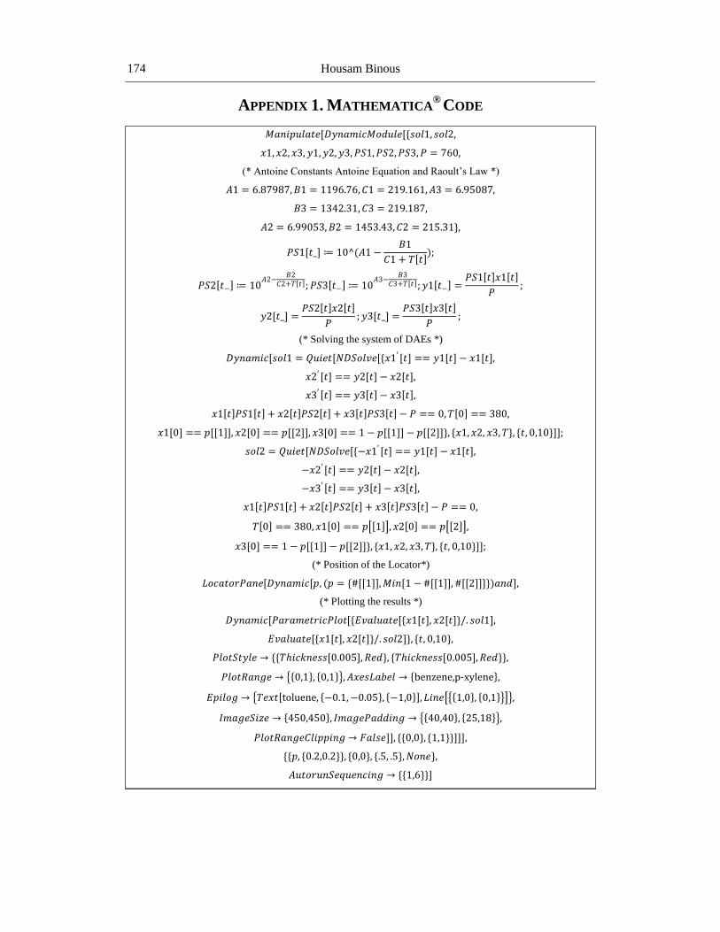
The full computer codes using both Mathematica®
and MATLAB® are given in the
Appendixes 1 and 2, respectively. Toluene, the intermediate-boiling component is a saddle
point. Benzene and p-xylene are the unstable and the stable nodes, respectively. The code
uses the built-in commands of MATLAB® and Mathematica®, ode15s and NDSolve,
respectively. Both commands can solve a system of differential algebraic equations (DAEs).
The differential equations are obtained by writing Eq. (1) for the three compounds and the
algebraic equation, which gives the bubble-temperature:
𝑃 = 𝑥1 𝑃1𝑠𝑎𝑡 + 𝑥2 𝑃2
𝑠𝑎𝑡 + 𝑥3 𝑃3𝑠𝑎𝑡 . (11)

Housam Binous 168
The code uses the new built-in Mathematica®
command, LocatorPane, to get the
coordinates of the computerřs mouse when user clicks the left button of the mouse:
𝐿𝑜𝑐𝑎𝑡𝑜𝑟𝑃𝑎𝑛𝑒[𝐷𝑦𝑛𝑎𝑚𝑖𝑐[𝑝, (𝑝 = {#[[1]],𝑀𝑖𝑛[1 − #[[1]], #[[2]]]})𝑎𝑛𝑑],
A small mathematical trick (in the command: 𝑀𝑖𝑛[1 − #[[1]], #[[2]]]) avoid having
mole fractions that are either negative or above 100%. An initial stillřs composition is
assigned these particular mouse coordinates. The code then integrates the system of DAEs for
this initial composition and draws the RC passing by this user-specified point.
The MATLAB® code operates in a similar manner and uses the built-in MATLAB®
command, ginput, in order to determine the initial stillřs composition, which corresponds to
the position of the computerřs mouse when the user clicks the left button of the mouse.
RC COMPUTATION FOR ETHANOL – WATER – ETHYLENE
GLYCOL MIXTURE
The tables 2, 3 and 4 give the modified Antoineřs constants and the data for the Wilson
model.
Table 2. Antoine’s constants for the water – ethanol – ethylene glycol mixture
(with F=2 and C=0).
A B D E
Water 65.9278 -7227.53 -7.17695 4.0313 e-6
Ethanol 86.4860 -7931.10 -10.2498 6.38949 e-6
Ethylene
glycol
57.9410 -8860.70 -5.71660 3.10800 e-6
Table 3. binary interaction parameters
for the water – ethanol – ethylene glycol mixture.
Water Ethanol Ethylene glycol
Water 0 276.75570 266.4848
Ethanol 975.48590 0 1539.411
Ethylene glycol 1043.84800 -129.2041 0
Table 4. molar volumes for the water – ethanol – ethylene glycol mixture.
Water 18.1
Ethanol 58.7
Ethylene glycol 55.9

Computation of Residue Curves Using Mathematica® and MATLAB® 169
Figure 5. RC for the water Ŕ ethanol Ŕ ethylene glycol mixture at 1 atm using Mathematica®.
Figure 6. Extractive distillation scheme for anhydrous ethanol production.
From the RCs (see Figure 5), it is clear that there is no distillation boundary since all RCs
start from the binary azeotrope (ethanol-water with 88% ethanol mole fraction) and end-up at
the ethylene glycol corner. Thus, the unique azeotrope is an unstable node; ethylene glycol is
0.0 0.2 0.4 0.6 0.8 1.0water0.0
0.2
0.4
0.6
0.8
1.0
ethanol
ethylene glycol
A

Housam Binous 170
a stable node and both ethanol and water are saddle point. Again, one can drag and place the
Locator at any position inside the triangle and the corresponding RC will be plotted
instantaneously.
Ethylene glycol can serve as an entrainer in order to perform extractive distillation (see
Figure 6) and obtain anhydrous ethanol. This can represent a good alternative to the well-
known three columns Kubierschky system using heteroazeotropic distillation and
cyclohexane as an entrainer.
RC COMPUTATIONS FOR THE HIGH PRESSURE CASE
Figure 7 shows a RC for the ternary system chloroform Ŕ acetone Ŕ methanol at P=10
atm. The tables 8, 9 and 10 give the modified Antoineřs constants and the data for the Wilson
model.
Table 8. Antoine’s constants for the chloroform – acetone – methanol mixture
(with F=2 and C=0)
A B D E
Chloroform 73.7 -6055.6 -8.9189 7.74407 e-6
Acetone 71.3 -5952. -8.531 7.82393 e-6
Methanol 59.83 -6282.8 -6.378 4.61746 e-6
Figure 7. RC for the chloroform Ŕ acetone Ŕ methanol mixture at 10 atm using Mathematica®.
0.0 0.2 0.4 0.6 0.8 1.0chloroform0.0
0.2
0.4
0.6
0.8
1.0
acetone
methanol A1
A2
A3
A4

Computation of Residue Curves Using Mathematica® and MATLAB® 171
Table 9. binary interaction parameters for the chloroform – acetone – methanol mixture
Chloroform Acetone Methanol
Chloroform 0 116.1171 1694.0240
Acetone -506.8518 0 551.4545
Methanol -361.7944 -124.932 0
Table 10. molar volumes for the chloroform – acetone – methanol mixture
Chloroform 80.7
Acetone 74.0
Methanol 40.7
The critical temperature and pressure and the acentric factor are given in Table 11.
Table 11. Critical temperature and pressure and the acentric factor for the
chloroform – acetone – methanol mixture.
𝑇𝐶 (°C) 𝑃𝐶 (kPa) 𝝎
Chloroform 263.2 5370 0.21796
Acetone 235.0 4700 0.30399
Methanol 239.4 7376 0.55699
Table 12. All azeotropes of the chloroform – acetone – methanol mixture at 10 atm.
Chloro-form acetone methanol bubble-point
𝑨𝟒: Chloroform-Acetone-
Methanol (saddle point)
6.66 % 29.17 % 64.17 % 402.35 K
𝑨𝟏: Chloroform-Methanol
(unstable node)
45.54 % 0 % 54.46 % 398.758 K
𝑨𝟑: Chloroform-Acetone
(stable node)
70.90 % 29.10 % 0 % 422.867 K
𝑨𝟐: Acetone-Methanol
(unstable node)
0 % 42.75 % 57.25 % 402.105 K
The compositions of the azeotropes and their corresponding bubble-temperature, at a
pressure equal to 10 atm, are given in Table 12. The three binary azeotropes are obtained as a
result of the RCM calculation. For the ternary azeotrope, accurate composition and bubble-
temperature computation required a separate calculation using the built-in command of
Mathematica®, FindRoot, which can find the solution of systems of nonlinear algebraic
equations.
The command that solves the system of DAEs is slightly different since it includes the
cubic equation, which solution is the compressibility factor:

Housam Binous 172
𝑁𝐷𝑆𝑜𝑙𝑣𝑒[{𝐷[𝑥1[𝑡], {𝑡, 1}] == 𝑦1[𝑡] − 𝑥1[𝑡],
𝐷[𝑥2[𝑡], {𝑡, 1}] == 𝑦2[𝑡] − 𝑥2[𝑡],
𝑥1 𝑡 + 𝑥2 𝑡 + 𝑥3 𝑡 == 1,𝑦1 𝑡 + 𝑦2 𝑡 + 𝑦3 𝑡 == 1,
𝑦1 𝑡 ==𝑥1 𝑡 𝑃𝑆𝑎𝑡1 𝑡 𝐺𝐴𝑀1 𝑡
𝑃𝜙 1 𝑡 ,
𝑦2 𝑡 ==𝑥2 𝑡 𝑃𝑆𝑎𝑡2 𝑡 𝐺𝐴𝑀2 𝑡
𝑃𝜙 2 𝑡 ,
𝑦3 𝑡 ==𝑥3 𝑡 𝑃𝑆𝑎𝑡3 𝑡 𝐺𝐴𝑀3 𝑡
𝑃𝜙 3 𝑡 ,
𝑍 𝑡 3 − 𝑍 𝑡 2 + 𝑍 𝑡 𝐴 𝑡 − 𝐵 𝑡 − 𝐵 𝑡 2 − 𝐴 𝑡 𝐵 𝑡 == 0,
𝑇 0 == 𝑇
. 𝑠𝑜𝑙1 , 𝑥1 0 == 𝑝 1 ,𝑥2 0 == 𝑝 2 ,
𝑥3 0 == 1 − 𝑝 1 − 𝑝 2 ,
𝑍 0 == 𝑍/. 𝑠𝑜𝑙1 ,𝑦1 0 == 𝑦1/. 𝑠𝑜𝑙1 ,𝑦2 0 == 𝑦2/. 𝑠𝑜𝑙1 ,
𝑦3[0] == (𝑦3/. 𝑠𝑜𝑙1)}, {𝑥1,𝑥2,𝑥3,𝑇,𝑍, 𝑦1,𝑦2,𝑦3}, {𝑡,−100,100}]
TEACHING DISTILLATION AND RCMS TO SENIOR
STUDENTS AT INSAT
Dr. Housam Binous started teaching RCM calculation at INSAT in 2002. A derivation of
Equations 1 and 3 is presented in the first lecture. VLE prediction is taught in a two-hour
separate lecture. Next, the author moves on to the application of RCMs in order to understand
complex distillation problems such as azeotropic, extractive and heteroazeotropic distillation
of ternary systems where one of the component is an entrainer. A brief discussion of entrainer
selection criteria is given too. In addition, separation of partially miscible mixtures such as the
n-butanol-water mixture using distillation column and decanters is presented. Finally, the
author usually ends this part of his course with a brief presentation of pressure swing
distillation and heat-integrated distillation columns. Since 2006, a four-hour computer
laboratory gives students hand-on experience on VLE data computation and RCMs
calculations using Mathematica®. Typical course enrollment was less than 50 students, all
majoring in chemical engineering. Students where split into four groups for the laboratory
sessions where they get hand-on experience using Mathematica® and MATLAB®. Students
usually have an important course load with all of them taking as much as six two-hour
lectures per week and a four-hour computing laboratory every other week. Feedback from
student was both generally very positive and very rewarding to the author; especially that our
senior students perceive the fact of obtaining in a couple of hours and without much difficulty
a residue curve for an ideal ternary mixture as a small academic achievement and a yet
another reason to gain confidence in their potentials.

Computation of Residue Curves Using Mathematica® and MATLAB® 173
CONCLUSION
In the present paper, several example of RC calculation were presented. Binary and
ternary mixtures were considered as well as ideal and non-ideal VLE behavior. Sample code,
given both in the text and in Appendixes 1-2, should make extension to other mixtures, with
or without liquid-phase chemical reaction, quite straightforward. The author hope that this
paper will help students and professionals alike to learn how to compute RCs and RCMs
using state-of-the-art computer programs such as Mathematica® and MATLAB®. Even
though, numerous commercial simulators such as DISTIL® and ASPEN
®, allow the
determination of RCM, it is useful to know how such computations are performed and how to
interpret the results that are obtained. All Mathematica® and MATLAB® code is available
upon request from the author or at the Wolfram Demonstration Project (Binous, 2009) and the
MATLAB® File Exchange Center (Binous, 2008).
ACKNOWLEDGMENTS
The support of King Fahd University of Petroleum and Minerals in duly acknowledged.
BIOGRAPHICAL INFORMATION
Dr. Housam Binous, a visiting Associate Professor at King Fahd University Petroleum
and Minerals, has been a full time faculty member at the National Institute of Applied
Sciences and Technology in Tunis for eleven years. He earned a Diplôme dřingénieur in
biotechnology from the Ecole des Mines de Paris and a Ph.D. in chemical engineering from
the University of California at Davis. His research interests include the applications of
computers in chemical engineering.
REFERENCES
[1] Binous H.; Wolfram Demonstration Project,
http://demonstrations.wolfram.com/author.html?author=Housam+Binous (2009)
[2] Binous H.; MATLAB® File Exchange Center,
http://www.mathworks.com/MATLABcentral/fileexchange/authors/11777 (2008)
[3] Doherty, M. F. and M. F. Malone, Conceptual Design of Distillation Systems, New
York: McGraw-Hill, 2001.
[4] Soave G., ŖEquilibrium constants from a modified Redlich-Kwong Equation of Stateŗ,
Chemical Engineering Science, Vol. 27, No. 6, pp. 1197-1203, 1972.
[5] Sandler, S. I., Chemical Engineering Thermodynamics, 3rd
Edition, NewYork: John
Wiley and Sons, 1999
[6] Wilson, G. M., ŖVapor-liquid equilibrium XI: a new expression for the excess free
energy of mixingŗ, Journal of the American Chemical Society, Vol. 86, pp. 127-130,
1964.
Housam Binous 174
APPENDIX 1. MATHEMATICA®
CODE
𝑀𝑎𝑛𝑖𝑝𝑢𝑙𝑎𝑡𝑒[𝐷𝑦𝑛𝑎𝑚𝑖𝑐𝑀𝑜𝑑𝑢𝑙𝑒[{𝑠𝑜𝑙1, 𝑠𝑜𝑙2,
𝑥1,𝑥2,𝑥3, 𝑦1,𝑦2,𝑦3,𝑃𝑆1,𝑃𝑆2,𝑃𝑆3,𝑃 = 760,
(* Antoine Constants Antoine Equation and Raoultřs Law *)
𝐴1 = 6.87987,𝐵1 = 1196.76,𝐶1 = 219.161,𝐴3 = 6.95087,
𝐵3 = 1342.31,𝐶3 = 219.187,
𝐴2 = 6.99053,𝐵2 = 1453.43,𝐶2 = 215.31},
𝑃𝑆1[𝑡_] ≔ 10^(𝐴1 −𝐵1
𝐶1 + 𝑇 𝑡 );
𝑃𝑆2 𝑡− ≔ 10𝐴2−
𝐵2𝐶2+𝑇 𝑡 ;𝑃𝑆3 𝑡− ≔ 10
𝐴3−𝐵3
𝐶3+𝑇 𝑡 ;𝑦1 𝑡− =𝑃𝑆1 𝑡 𝑥1 𝑡
𝑃;
𝑦2[𝑡_] =𝑃𝑆2 𝑡 𝑥2 𝑡
𝑃;𝑦3[𝑡_] =
𝑃𝑆3 𝑡 𝑥3 𝑡
𝑃;
(* Solving the system of DAEs *)
𝐷𝑦𝑛𝑎𝑚𝑖𝑐[𝑠𝑜𝑙1 = 𝑄𝑢𝑖𝑒𝑡[𝑁𝐷𝑆𝑜𝑙𝑣𝑒[{𝑥1′ [𝑡] == 𝑦1[𝑡] − 𝑥1[𝑡],
𝑥2′ [𝑡] == 𝑦2[𝑡] − 𝑥2[𝑡],
𝑥3′ 𝑡 == 𝑦3 𝑡 − 𝑥3 𝑡 ,
𝑥1 𝑡 𝑃𝑆1 𝑡 + 𝑥2 𝑡 𝑃𝑆2 𝑡 + 𝑥3 𝑡 𝑃𝑆3 𝑡 − 𝑃 == 0,𝑇 0 == 380,
𝑥1[0] == 𝑝[[1]], 𝑥2[0] == 𝑝[[2]], 𝑥3[0] == 1 − 𝑝[[1]] − 𝑝[[2]]}, {𝑥1,𝑥2, 𝑥3,𝑇}, {𝑡, 0,10}]];
𝑠𝑜𝑙2 = 𝑄𝑢𝑖𝑒𝑡[𝑁𝐷𝑆𝑜𝑙𝑣𝑒[{−𝑥1′ [𝑡] == 𝑦1[𝑡] − 𝑥1[𝑡],
−𝑥2′ [𝑡] == 𝑦2[𝑡] − 𝑥2[𝑡],
−𝑥3′ 𝑡 == 𝑦3 𝑡 − 𝑥3 𝑡 ,
𝑥1 𝑡 𝑃𝑆1 𝑡 + 𝑥2 𝑡 𝑃𝑆2 𝑡 + 𝑥3 𝑡 𝑃𝑆3 𝑡 − 𝑃 == 0,
𝑇 0 == 380,𝑥1 0 == 𝑝 1 , 𝑥2 0 == 𝑝 2 ,
𝑥3[0] == 1 − 𝑝[[1]] − 𝑝[[2]]}, {𝑥1,𝑥2,𝑥3,𝑇}, {𝑡, 0,10}]];
(* Position of the Locator*)
𝐿𝑜𝑐𝑎𝑡𝑜𝑟𝑃𝑎𝑛𝑒[𝐷𝑦𝑛𝑎𝑚𝑖𝑐[𝑝, (𝑝 = {#[[1]],𝑀𝑖𝑛[1 − #[[1]], #[[2]]]})𝑎𝑛𝑑],
(* Plotting the results *)
𝐷𝑦𝑛𝑎𝑚𝑖𝑐[𝑃𝑎𝑟𝑎𝑚𝑒𝑡𝑟𝑖𝑐𝑃𝑙𝑜𝑡[{𝐸𝑣𝑎𝑙𝑢𝑎𝑡𝑒[{𝑥1[𝑡], 𝑥2[𝑡]}/. 𝑠𝑜𝑙1],
𝐸𝑣𝑎𝑙𝑢𝑎𝑡𝑒[{𝑥1[𝑡], 𝑥2[𝑡]}/. 𝑠𝑜𝑙2]}, {𝑡, 0,10},
𝑃𝑙𝑜𝑡𝑆𝑡𝑦𝑙𝑒 → {{𝑇𝑖𝑐𝑘𝑛𝑒𝑠𝑠[0.005],𝑅𝑒𝑑}, {𝑇𝑖𝑐𝑘𝑛𝑒𝑠𝑠[0.005],𝑅𝑒𝑑}},
𝑃𝑙𝑜𝑡𝑅𝑎𝑛𝑔𝑒 → 0,1 , 0,1 ,𝐴𝑥𝑒𝑠𝐿𝑎𝑏𝑒𝑙 → benzene,p-xylene ,
𝐸𝑝𝑖𝑙𝑜𝑔 → 𝑇𝑒𝑥𝑡 toluene, −0.1,−0.05 , −1,0 ,𝐿𝑖𝑛𝑒 1,0 , 0,1 ,
𝐼𝑚𝑎𝑔𝑒𝑆𝑖𝑧𝑒 → 450,450 , 𝐼𝑚𝑎𝑔𝑒𝑃𝑎𝑑𝑑𝑖𝑛𝑔 → 40,40 , 25,18 ,
𝑃𝑙𝑜𝑡𝑅𝑎𝑛𝑔𝑒𝐶𝑙𝑖𝑝𝑝𝑖𝑛𝑔 → 𝐹𝑎𝑙𝑠𝑒]], {{0,0}, {1,1}}]]],
{{𝑝, {0.2,0.2}}, {0,0}, {.5, .5},𝑁𝑜𝑛𝑒},
𝐴𝑢𝑡𝑜𝑟𝑢𝑛𝑆𝑒𝑞𝑢𝑒𝑛𝑐𝑖𝑛𝑔 → {{1,6}}]

Computation of Residue Curves Using Mathematica® and MATLAB® 175
APPENDIX 2. MATLAB® CODE
h=figure(1);
line([0 1],[1 0])
axis([0 1 0 1])
hold on
button = questdlg('do you want to draw a residue curve',...
'','yes','no','yes');
while (button(1)=='y')
% determination of the position of the mouse
[x y]=ginput(1);
if x<0
x=max(x,0);
end;
if y<0
y=max(0,y);
end;
if y+x>1
y=min(1-x,y);
end;
% Solving the system of DAEs
opts = odeset('Mass','M','MassSingular','yes');
[t X]=ode15s('RCM1',[0 10],[x y 1-x-y 350],opts);
% plotting the residu curve
plot(X(:,1),X(:,2),'r')
[t X]=ode15s('RCM2',[0 10],[x y 1-x-y 350],opts);
plot(X(:,1),X(:,2),'r')
button = questdlg('do you want to draw a residue curve','',...
'yes','no','yes');
APPENDIX 2. MATLAB® CODE (Continued)
end
close(h)
function xdot=RCM1(t,x,flag)
if isempty(flag),

Housam Binous 176
T=x(4);
% Total Pressure
P=760;
% Antoine constants
A1=6.87987;B1=1196.76;C1=219.161;
A2=6.99053;B2=1453.43;C2=215.310;
A3=6.95087;B3=1342.31;C3=219.187;
% Antoine Equation
PS1=10^(A1-B1/(C1+T));
PS2=10^(A2-B2/(C2+T));
PS3=10^(A3-B3/(C3+T));
% Raoultřs Law
y1=PS1*x(1)/P;
y2=PS2*x(2)/P;
y3=PS3*x(3)/P;
% System of DAEs
xdot(1)=x(1)-y1;
xdot(2)=x(2)-y2;
xdot(3)=x(3)-y3;
xdot(4)=y1+y2+y3-1;
xdot = xdot'; % xdot must be a column vector
else
% Return M
M = zeros(4,4);
M(1,1) = 1;
M(2,2) = 1;
M(3,3) = 1;
xdot = M;
end
Recommended